Ground and excited charmonium state production in $p$+$p$ collisions at $\sqrt{s}=$ 200 GeV

Abstract

We report on charmonium measurements [$J/\psi$ (1S), $\psi^{\prime}$ (2S), and $\chi_{c}$ (1P)] in $p$+$p$ collisions at $\sqrt{s}=$ 200 GeV. We find that the fraction of $J/\psi$ coming from the feed-down decay of $\psi^{\prime}$ and $\chi_{c}$ in the midrapidity region ($|\eta|<0.35$) is 9.6 $\pm$ 2.4% and 32 $\pm$ 9%, respectively. New, higher statistics $p_{T}$ and rapidity dependencies of the $J/\psi$ yield via dielectron decay in the same midrapidity range and at forward rapidity ($1.2<|\eta|<2.4$) via dimuon decay are also reported. These results are compared with measurements from other experiments and discussed in the context of current charmonium production models.

I Introduction

Since its discovery, charmonium (bound $c\bar{c}~{}$states) has been proposed as a powerful tool to investigate many aspects of QCD such as the distribution of partons in protons and nuclei at large momentum transfer. Charm quarks are predominantly produced in gluon interactions at $\sqrt{s}=$ 200 GeV, therefore they are sensitive to the gluon distribution in the nucleon and its modification in the nucleus. In addition, the color screening of the $c\bar{c}~{}$state makes charmonium dissociation an important signature for the formation of a deconfined state of matter created in A+A collisionsMatsui and Satz (1986); Mócsy and Petreczky (2007). Such studies rely on a accurate understanding of charmonium production in $p$+$p$ collisions which is the goal of the present work.

The cross section of $c\bar{c}~{}$production is known from pQCD calculations to about a factor of two compared to PHENIX data Cacciari et al. (2005); Adare et al. (2006a). However, the hadronization step which forms the bound state is a nonperturbative process and is not well understood. A variety of schemes have been proposed, some of the most common being the Color Evaporation Model (CEM), the Color Singlet Model (CSM) and nonrelativistic quantum chromodynamics (NRQCD), also known as the Color Octet Model (COM). We review these models briefly here, and compare to them later in the text.

In the CEM Fritzsch (1977); Amundson et al. (1997) the bound-state production mechanism is insensitive to the $c\bar{c}~{}$quantum numbers. The $c\bar{c}~{}$pair is produced as long as the center of mass energy of the pair, $\sqrt{\hat{s}}$, is greater than the mass of two charm quarks, but less than the mass of two open charm mesons. Charmonium states are then color neutralized during the hadronization process by soft gluon emission. The yield of different charmonium states is a fixed fraction $\mathcal{F}$ of the integrated pQCD $c\bar{c}~{}$cross section. $\mathcal{F}$ is determined from experiments and is universal. Hence in this model, the ratio between the yield of different charmonium states is momentum and energy independent.

In the CSM Baier and Ruckl (1981) the production amplitude of on-shell $c\bar{c}~{}$pairs is projected onto ${}^{2S+1}L_{J}$ angular momentum states, and hence accounts for the $J/\psi~{}$and $\psi^{\prime}~{}$as ${}^{3}S_{1}$ and the $\chi_{c}$ states as ${}^{3}P_{0,1,2}$. The model assumes that these charmonium states are formed in their final color singlet quantum number configuration. The production density matrix is coupled to the wave function at the origin which is determined from potential models. The only empirical parameters entering in the entire calculation are the leptonic decay width and the charmonium mass used in the potential model.

NRQCD allows for the production of both color singlet and color octet $c\bar{c}~{}$states. Color octet states emit one or more gluons during hadronization in order to neutralize their color. The production amplitude is expanded in powers of both the strong coupling, $\alpha_{S}$, and the velocity, $\nu$, of the heavy quarks relative to the $c\bar{c}~{}$pair. The expansion in $\nu$ assumes that the heavy quark is nonrelativistic. As in the CSM, the production amplitudes are projected onto ${}^{2S+1}L_{J}$ states. Since the potential model can only be applied to the color singlet state, a long range nonperturbative matrix element for each quarkonium state is fitted from experiments. The earliest such matrix parametrization Cho and Leibovich (1996) was tuned with $J/\psi~{}$and $\psi^{\prime}~{}$cross sections observed in CDF ($\sqrt{s}$ = 1.8 TeV) Abe et al. (1997a) which indicated that while P-wave charmonium ($\chi_{c}$ ) has no important color octet state contributions, S-wave charmonium (direct $J/\psi~{}$and $\psi^{\prime}~{}$) production is largely through color octet channels. Therefore, this model is sometimes simply referred to as the Color Octet Model (COM).

Each model has its strengths and weaknesses. The CEM is able to reasonably describe quarkonia yields observed in many experiments, but has no predictive power for $c\bar{c}~{}$polarization. Cross sections calculated using CSM grossly underestimate the yields observed at PHENIX Adare et al. (2007a) and at CDF Abe et al. (1997a). Recent next-to-leading order (NLO) Campbell et al. (2007); Artoisenet et al. (2007); Gong and Wang (2008) and next-to-next-leading order (NNLO) Artoisenet et al. (2008); Lansberg (2009a, b, 2010) calculations for the color singlet states resulted in significant modifications of the predicted charmonium yields and polarization, but not sufficient to agree with the experimental results. NRQCD tuned with $J/\psi~{}$and $\psi^{\prime}~{}$$p_{T}$ spectra from CDF was able to qualitatively describe the first PHENIX $J/\psi~{}$cross section and polarization results Adare et al. (2010a) albeit with large experimental uncertainties, but failed to describe the $J/\psi~{}$and $\psi^{\prime}~{}$polarization observed in CDF Abulencia et al. (2007) (see Lansberg (2009a) for a recent review). Recent NRQCD calculations Butenschön and Kniehl (2011) include color singlet and color octet NLO short range terms along with a long-range matrix parametrization from experimental hadroproduction Acosta et al. (2005) and photoproduction Adloff et al. (2002); Aaron et al. (2010) of $J/\psi~{}$mesons. However, the NLO terms for the color octet Gong et al. (2009) have only small corrections compared to the leading-order (LO) terms and the calculations still disagree with the $J/\psi~{}$polarization measured by CDF.

One of the complications in the $J/\psi~{}$total cross section and polarization calculations (observables where experimental tests are readily available) is the contribution from the decays of excited charmonium states, primarily $\psi^{\prime}$, $\chi_{c1}$ and $\chi_{c2}$. In addition, the $J/\psi~{}$suppression observed in heavy ion collisions cannot be completely understood without a knowledge of the feed-down fraction of excited charmonium state decays to the $J/\psi$. This is particularly true under the assumption that the suppression is due to the disassociation of charmonium in the a high temperature quark-gluon plasma, since lattice calculations Mócsy and Petreczky (2007) indicate that the melting points of the $\chi_{c}$ and $\psi^{\prime}~{}$states are lower than that of the $J/\psi~{}$. In this work the feed-down fractions to the $J/\psi~{}$from excited charmonium states is measured since they can be determined more precisely than production cross sections as many of the systematic uncertainties cancel when making cross section ratios.

The PHENIX Experiment at RHIC can measure quarkonia dilepton decays over a broad $p_{T}$ and rapidity range and can detect photons from $\chi_{c}$ radiative decays using electromagnetic calorimeters at midrapidity. This article reports on the feed-down fraction of the $J/\psi~{}$yield which comes from $\psi^{\prime}~{}$and $\chi_{c}$ decays at midrapidity in $p$+$p$ collisions at $\sqrt{s}=$ 200 GeV. For these we used the $\psi^{\prime}~{}$to $J/\psi~{}$yield ratio in the dielectron channel and the full reconstruction of the $\mbox{$p$+$p$~{}}\rightarrow\mbox{$\chi_{c}$~{}}\rightarrow\mbox{$J/\psi~{}$}+\gamma\rightarrow e^{+}e^{-}+\gamma$ decay. A new $J/\psi~{}$differential cross section measurement at midrapidity and forward rapidity using the increased luminosity obtained in the 2006 and 2008 runs, is also presented. These provide more accurate measurements than previously published in Adare et al. (2007a), particularly for the $J/\psi~{}$differential cross section at high $p_{T}$ . The results obtained in these analyses also provide a baseline for the study of $J/\psi~{}$suppression in $d$+Au Adare et al. (2010b) and Au+Au Adare et al. (2011, 2007b) collisions at PHENIX.

Systematic uncertainties throughout this article are classified according to whether or not there are point-to-point correlations between the uncertainties. Type A systematic uncertainties are point-to-point uncorrelated, similar to statistical uncertainties, since the points fluctuate randomly with respect to each other. Type B systematic uncertainties are point-to-point correlated. The points fluctuate coherently with respect to each other. That is, it accounts for the uncertainty in the nth-order derivative of the measured spectrum, in most cases the slope. Global, or type C, systematics are those where all points fluctuate in the same direction and by the same fractional amount.

The remainder of the article is arranged as follows. An introduction to the PHENIX detector, a description of the data sample, and a description of the lepton identification method is described in Sec. II. The analysis is described in three sections: midrapidity $J/\psi~{}$and $\psi^{\prime}~{}$dielectron cross section measurement in the PHENIX central arms (Sec. III); direct $\chi_{c}$ feed-down measurement in the central arms (Sec. IV); and forward rapidity $J/\psi~{}$cross section measurement in the muon arms (Sec. V). The results are compared to measurements from other experiments and to current theoretical calculations in Sec. VI.

II Experimental Apparatus and the Data Set

The PHENIX detector Adcox et al. (2003) is composed of four arms. Two central arms measure electrons, photons and hadrons over $|\eta|<0.35$ with each azimuthally covering $\Delta\phi=\pi/2$. Two forward muon arms measure muons over the range $-2.2<\eta<-1.2$ arm and $1.2<\eta<2.4$ with full azimuthal coverage.

Charged particle tracks in the central arms are formed using the Drift Chamber (DCH), the Pad Chamber (PC) and the collision point. Electron candidates required at least one fired phototube within an annulus 3.4 $<R_{ring}[cm]<$ 8.4 centered on the projected track position on the Ring Imaging Čerenkov detector (RICH). In addition, the electron candidate is required to be associated with an energy cluster in the Electromagnetic Calorimeter (EMCal) that falls within 4$\sigma_{position}$ of the projected track position, and within 4$\sigma_{energy}$ of the expected energy/momentum ratio where the $\sigma$’s characterize the position and energy resolution of the EMCal. The relatively loose association requirement still provides excellent hadron rejection due to the very small particle multiplicity in $p$+$p$ collisions. Based on the $p_{T}$ range of decay electrons from $J/\psi~{}$observed in real data and simulations, a minimum $p_{T}$ of 500 MeV/$c$ was also required for each electron candidate.

Each of the forward muon armsAkikawa et al. (2003) comprises a hadron absorber, three stations of cathode strip chambers for particle tracking (MuTr), and a Muon Identifier detector (MuID). The hadron absorber is composed of a 20 cm thick copper nosecone and 60 cm of iron which is part of the magnet. The MuTr is installed in an eight-sided conical magnet. The MuID is composed of five steel hadron absorbers interleaved with six panels of vertical and horizontal Iarocci tubes. A single muon needs a longitudinal momentum of 2 GeV/$c~{}$to reach the most downstream MuID plane. Tracks reconstructed in the MuTr are identified as muons if they match a “road” formed by hits in the MuID, within 2.5$\sigma$ of angular resolution. At least one tube in the last MuID plane should have fired. Additional cuts include a $\chi^{2}<23$ for the reconstructed track, a $\chi^{2}<9$ for the track projection to the collision vertex and a polar angle cut of $14^{\circ}<\theta_{\mu}<33^{\circ}$ for the north arm and $147^{\circ}<\theta_{\mu}<166^{\circ}$ for the south arm to avoid acceptance inconsistencies between the detector simulation and real data near the edges of the muon arms.

Beam interactions were selected with a minimum-bias (MB) trigger that requires at least one hit per beam crossing in each of the two beam-beam counters (BBC) placed at $3.0<|\eta|<3.9$. Studies using Vernier scans (also called van der Meer scans) Adler et al. (2003) conclude that this MB trigger accepts a cross section of $\sigma_{\rm BBC}$ = 23.0 $\pm$ 2.2 mb. This cross section represents 55 $\pm$5% of the $\sigma_{pp}^{inel.}$ = 42 $\pm$ 3 mb $p$+$p$ inelastic cross section at $\sqrt{s}=$ 200 GeV.

Dedicated triggers were used to select events with at least one electron or two muon candidates. An EMCal RICH Trigger (ERT) required a minimum energy in any 2$\times$2 group of EMCal towers, corresponding to $\Delta\eta\times\Delta\phi=0.02\times 0.02$ rad., plus associated hits in the RICH. The minimum EMCal energy requirement was 400 MeV for the first half of the Run and 600 MeV for the second half. The data used in this analysis were taken with the ERT in coincidence with the MB trigger. Events were also triggered when there were two muon candidates in one of the MuID arms. The trigger logic for a muon candidate required a “road” of fired Iarocci tubes in at least four planes, including in the most downstream plane relative to the collision point. The event sample used in the dimuon analysis required a MuID trigger in coincidence with the MB trigger.

There are events which produce a $J/\psi~{}$but do not fire the MB trigger. The fraction, $\varepsilon_{inel.}$,of such events is estimated by measuring the number of high $p_{T}$ $\pi^{0}\rightarrow\gamma\gamma$ decays which satisfy the minimum energy condition of the ERT and which do not satisfy the MB trigger. It was found that $\varepsilon_{inel.}=(79\pm 2)\%$. The correction due to this factor is included in all cross section calculations for measurements requiring the MB trigger. No dependence of $\varepsilon_{inel.}$ on the $p_{T}$ of the measured $\pi^{0}$ decays was found over the range 0-10 GeV/$c~{}$Adare et al. (2010c).

The collision point along the beam direction is determined with a resolution of 1.5 cm by using the difference between the fastest time signals measured in the north and south BBC detectors. The collision point was required to be within $\pm$30 cm of the nominal center of the detector. In the dielectron analysis, runs in which electron yields were more than three standard deviations away from the average in at least one of the eight EMCal azimuthal sectors, were discarded. For the dimuon analysis, runs where the muon arm spectrometers were not fully operational were rejected.

The 2006 data sample used in the dielectron analysis corresponded to $N_{pp}=$ 143 billion minimum bias events, or an integrated luminosity of $\int\mathcal{L}dt=N_{pp}/\sigma_{\rm BBC}=(6.2\pm 0.6)$ pb^-1. The 2006 and 2008 data samples used for the muon analysis, corresponded to 215 billion minimum bias events, or a luminosity of $(9.3\pm 0.9)$ pb^-1.

III $J/\psi~{}$and $\psi^{\prime}~{}$analysis in the midrapidity region

The procedure for analyzing the $J/\psi~{}$and $\psi^{\prime}~{}$$\rightarrow$ dielectron signal in the central arm detectors is detailed in this section. The overall procedure to select dielectrons and extract the charmonium signal and determine combinatorial and correlated backgrounds is explained in III.1. Studies of the central arm detector response to charmonium dielectron decays is the subject of the section III.2. The final $p_{T}$ and rapidity dependence of the cross sections is calculated in Section III.3 together with a summary of all systematic uncertainties mentioned throughout the text. Finally the $\psi^{\prime}$/($J/\psi~{}$) dielectron yield ratio is calculated in Section III.4.

III.1 Di-electron decays of $J/\psi~{}$and $\psi^{\prime}~{}$mesons in the midrapidity region.

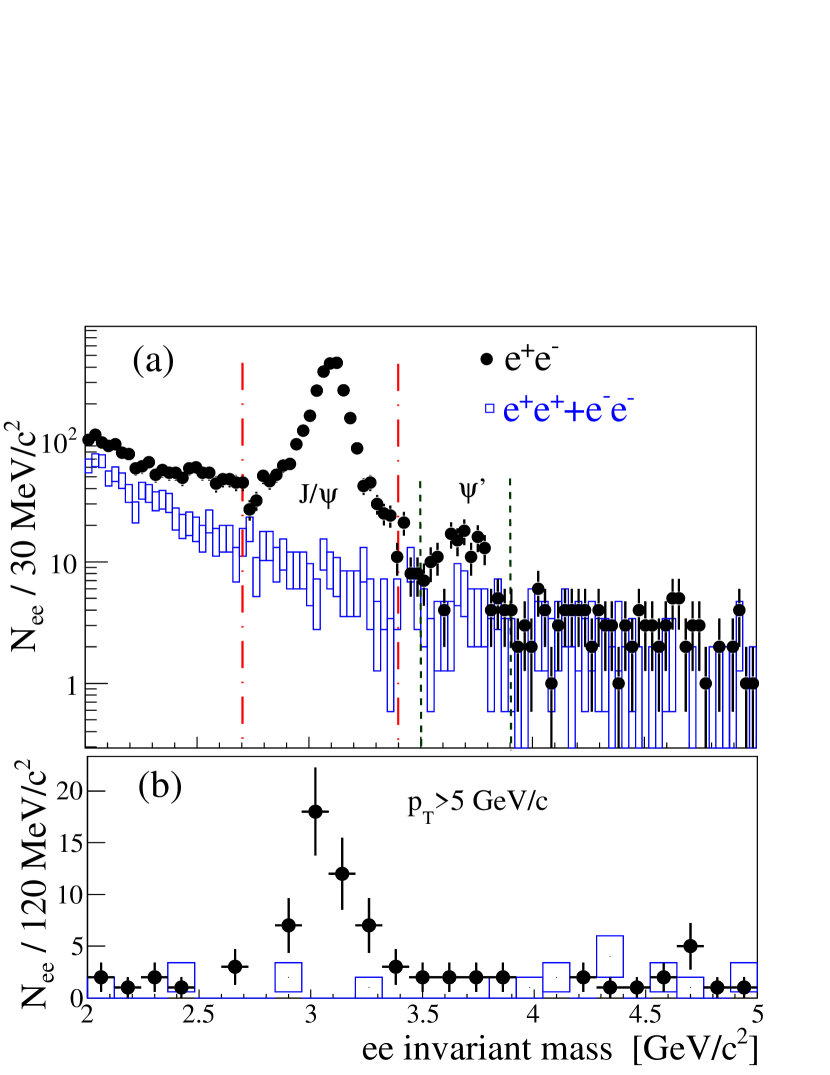
Figure 1: (Color online) Invariant mass distribution of unlike-sign (closed circles) and like-sign (open boxes) dielectrons in the $J/\psi~{}$and $\psi^{\prime}~{}$region without (a) and with (b) a minimum $p_{T}$ requirement for the dielectron pair. Dash-dotted (dashed) lines represent the mass range used to count $J/\psi~{}$($\psi^{\prime}~{}$) decays.

The invariant mass was calculated for all electron pairs in which one electron of the pair geometrically matched the position of a fired ERT segment. This requirement was necessary given that we used simulated $J/\psi~{}$and $\psi^{\prime}~{}$decays to estimate the ERT efficiency. Di-electron contributions to $J/\psi~{}$and $\psi^{\prime}~{}$decays are clearly identified as peaks in this invariant mass distribution (Fig. 1). The primary sources of physically correlated unlike-sign pairs ($e^{+}e^{-}$) are quarkonia decays, open $c\bar{c}~{}$and $b\bar{b}~{}$pairs, Drell-Yan, and jets. Uncorrelated unlike-sign pairs are from combinatorial background. The primary sources of like-sign pairs ($e^{+}e^{+}+e^{-}e^{-}$) are combinatorial background, and electrons from particle decays occurring in the same jet (mostly $\pi^{0}$ Dalitz decays). The like-sign pair mass distribution normalized by the geometric mean of the number of $e^{+}e^{+}$ and $e^{-}e^{-}$ pairs was statistically subtracted from the unlike-sign mass distribution. The primary effect of this subtraction was to account for combinatorial background, however it also accounted for much of the jet background. There are 2882 unlike-sign and 203 like-sign dielectrons in the $J/\psi~{}$mass range (2.7$<M_{ee}[\mbox{GeV/$c^{2}~{}$}]<$3.4), giving a correlated signal of 2,679 $\pm$ 56 counts and a signal/background of 13. In the $\psi^{\prime}~{}$mass region (3.5$<M_{ee}[\mbox{GeV/$c^{2}~{}$}]<$3.9) there were 137 unlike-sign and 51 like-sign electron pairs corresponding to a signal of 86 $\pm$ 14 counts and signal/background of 1.7.

The jet contribution in the charmonium mass region is three orders of magnitude smaller than from the $J/\psi~{}$and $\psi^{\prime}~{}$with a steeply falling mass spectrumAdare et al. (2010d) and will be ignored here; in any case it is largely removed by the like-sign subtraction. The Drell-Yan contribution was estimated using next-to-leading-order calculations Vogelsang (2007). Taking into account the detector acceptance, the fraction of the dielectron signal which comes from Drell-Yan processes is 0.23 $\pm$ 0.03 % in the $J/\psi~{}$mass region and 3.37 $\pm$ 0.40 % in the $\psi^{\prime}~{}$region. The heavy quark contribution is the major background to the correlated dielectron spectrum. In fact, they represent a significant fraction of the correlated dielectrons in the $\psi^{\prime}~{}$mass region. They will be estimated by two models as described in the next several paragraphs.

In order to understand the dielectron spectrum, a simulation was done for the three primary contributions to the mass spectrum: the $J/\psi~{}$and $\psi^{\prime}$, heavy quark pairs, and Drell-Yan. The first step was to generate the initial correlated electron pair spectrum. The $J/\psi~{}$and $\psi^{\prime}~{}$were generated by weighting their distributions in order to obtain the same $p_{T}$ spectrum as seen in real data. The $J/\psi~{}$radiative decay ($\mbox{$J/\psi~{}$}\rightarrow\mbox{$e^{+}e^{-}$~{}}+\gamma$), also called internal radiation, was introduced using the mass distribution estimated from QED calculations Spiridonov (2004). Drell-Yan pairs were generated according to the mass distribution obtained from NLO calculations. In order to make a conservative estimate and determine whether the result is model independent, the $c\bar{c}~{}$and $b\bar{b}~{}$mass distributions were obtained using two different methods:

1. A dielectron generator: The semi-leptonic heavy flavor yield measured in Adare et al. (2010c, 2006b) was split into the $c\bar{c}~{}$($d\sigma_{c\bar{c}}/dp_{T}$) and $b\bar{b}~{}$($d\sigma_{b\bar{b}}/dp_{T}$) distributions according to the $c/b$ ratio from fixed-order plus next-to-leading-log (FONLL) calculations Cacciari et al. (2005) which agree with PHENIX measurements of separated $c\bar{c}~{}$and $b\bar{b}~{}$productionAdare et al. (2009a); Aggarwal et al. (2010). These $c\bar{c}~{}$and $b\bar{b}~{}$yields were used as input for an electron Monte Carlo generator with uniform rapidity distribution ($|y|<0.5$) and the measured vertex distribution. An electron and positron from the decay of a heavy quark pair were generated for each event. In this method the heavy quarks are assumed to have no angular correlation.

2. pythia: Hard scattering collisions were simulated using the pythiaSjostrand et al. (2006) generator. Leading order pair creation sub-processes and next-to-leading-order flavor creation and gluon splitting sub-processes are all included in the heavy quark generation Norrbin and Sjostrand (2000). These sub-processes have different opening angles for the heavy quark pair. The simulation used the CTEQ6M Pumplin et al. (2002) parton distribution functions (PDF), a Gaussian $k_{T}=$ distribution of width 1.5 GeV/$c~{}$, a charm quark mass of 1.5 GeV and bottom quark mass of 4.8 GeV. Variations of the $k_{T}$ distribution and masses of the heavy quarks were included in the systematic uncertainties. The $p_{T}$ dependence of electrons from $c\bar{c}~{}$and $b\bar{b}~{}$given by the simulation agrees with the PHENIX measurement of single electrons from heavy flavor decayAdare et al. (2010c).

The generated electron pairs from all sources were then used as input to a geant-3 GEA based detector Monte-Carlo which included effects such as Bremsstrahlung radiation of electrons when crossing detector material and air (external radiation). Simulated events were then reconstructed and analyzed using the same criteria as were used for real data and reported in Sec.II and Sec.III.1. More details will be given later in Sec.III.2, including methods of estimating systematic errors.

The resulting simulated distributions were then fit to the 2-dimensional mass vs $p_{T}$ distribution of the measured dielectron signal in the mass range $2.0<M_{e^{+}e^{-}}[\mbox{GeV/$c^{2}~{}$}]<8.0$. The fit parameters included the normalization of $c\bar{c}~{}$, $b\bar{b}~{}$, $J/\psi~{}$and $\psi^{\prime}~{}$contributions, the fraction of the internal radiation, and a mass resolution correction for the simulated resonance peaks. The normalization of the Drell Yan was fixed according to expectations from the NLO calculations.

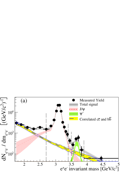
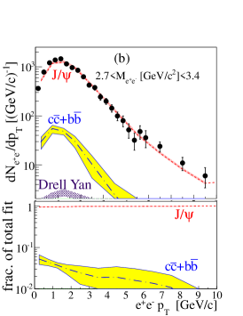
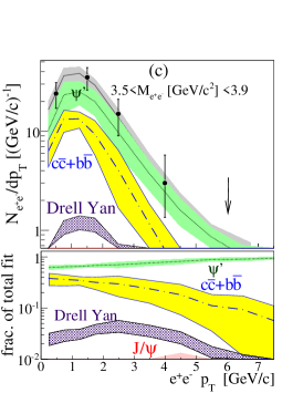
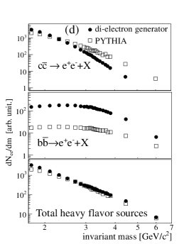
Figure 2: (Color online) Correlated dielectron mass (a) and $p_{T}$ distributions in the $J/\psi~{}$(b) and $\psi^{\prime}~{}$(c) mass regions. Signal components were estimated by fitting open heavy flavor, Drell Yan (normalization fixed by NLO calculations), $J/\psi~{}$and $\psi^{\prime}~{}$decays after detector simulation. The $c\bar{c}~{}$and $b\bar{b}~{}$components were generated using pythia Sjostrand et al. (2006) and a heavy flavor based dielectron generator described in the text. Bands correspond to the type A fitting uncertainties and the type B systematic uncertainty obtained when using the two different open heavy quark generators. Panel (d) shows the result after the fit for $c\bar{c}$, $b\bar{b}~{}$and total open heavy flavor components from each generator.

Fig. 2 shows the results of the fit for the dielectron mass (a) and $p_{T}$ (b,c). The heavy flavor contribution to the continuum obtained from the fit using the dielectron generator and pythia is shown in Fig. 2-d. When using the pythia simulation, the presence of back-to-back correlated $c\bar{c}~{}$and $b\bar{b}~{}$pairs produced more high mass pairs per $c\bar{c}~{}$which then forced a smaller contribution from $b\bar{b}$. As can be seen from the figure, the fits performed using the two generators give very different normalizations for the open charm and the open bottom contributions. However, the two methods give very similar contributions for the sum which is well constrained by data. Thus the lack of the knowledge of the angular correlation in heavy flavor production does not affect the estimate of the total continuum contribution from open heavy flavor in the $J/\psi~{}$and $\psi^{\prime}~{}$mass regions. The measurement of the $c\bar{c}~{}$and $b\bar{b}~{}$cross sections is not in the scope of this paper; a more detailed study can be found in Adare et al. (2009b, c); Aggarwal et al. (2010). Type A fit parameter uncertainties and the type B uncertainty obtained from the difference in results obtained using the two generators for the total heavy flavor contribution, are summed in quadrature and shown as bands in Fig. 2. Values for the fraction of the charmonium signal $\left(f_{\psi}\right)$ shown in Figs. 2-b and 2-c are used later in the yield calculation.

The fitted external and internal radiation contributions indicate that the fraction of radiative decays of the $J/\psi~{}$, where the undetected photon has energy larger than 100 MeV, is (9 $\pm$ 5)%. This is consistent with QED calculations which indicate that 10.4% of the dielectron decays from the $J/\psi~{}$come from such radiative decays and a measurement of fully reconstructed $J/\psi\rightarrow e^{+}e^{-}\gamma$ performed by E760 Armstrong et al. (1996) which gives 14.7 $\pm$ 2.2 %. The $J/\psi~{}$mass peak around 3.096 GeV/$c^{2}~{}$has a Gaussian width from the fit of 53 $\pm$ 4 MeV after including a mass resolution in the MC of ($\delta M/M$) of (1.71 $\pm$ 0.13)%. Because of the radiative tails, the mass range (2.7$<M_{ee}[\mbox{GeV/$c^{2}~{}$}]<$3.4) contains $\varepsilon_{mass}^{J/\psi}=93.8\pm 0.9$% of the $J/\psi~{}$decays and the mass region (3.5$<M_{ee}[\mbox{GeV/$c^{2}~{}$}]<$3.9) contains $\varepsilon_{mass}^{\psi^{\prime}}=86\pm 2$% of the $\psi^{\prime}~{}$decays, corrections included in the yield calculations. The foreground yield as well as the statistical uncertainties used in the cross section calculations were obtained assuming that both foreground and background distributions are independent and follow Poisson statistics. The total foreground was then multiplied by the factors obtained from fits in the previous section to obtain the $J/\psi~{}$and $\psi^{\prime}~{}$yields. In each bin of $p_{T}$ (or y) the foreground signal $(\mu_{f})$ was obtained from the unlike-sign counts $(fg)$ in the distribution and the background $(\mu_{b})$ was obtained from the like-sign counts $(bg)$ (Fig. 1 top). The joint probability distribution for the net number of counts $s=\mu_{f}-\mu_{b}$ is

$$P(s,\mu_{b})=\frac{\mu_{b}^{bg}}{bg!}\frac{\mu_{b}^{fg}}{fg!}e^{-2\mu_{b}}\left(1+\frac{s}{\mu_{b}}\right)^{fg}e^{-s}.$$ (1)

We expand the term $\left(1+\frac{s}{\mu_{b}}\right)^{fg}$:

$$\left(1+\frac{s}{\mu_{b}}\right)^{fg} = \sum_{k=0}^{fg}\frac{fg!}{(fg-k)!k!}\left(\frac{s}{\mu_{b}}\right)^{k}$$ (2)

$$P(s,\mu_{b}) = \sum_{k=0}^{n}\frac{\mu_{b}^{bg+fg-k}e^{-2\mu_{b}}}{bg!(fg-k)!}\frac{s^{k}e^{-s}}{k!}.$$

Assuming no negative signal, the expression is summed over $\mu_{b}$ from 0 to $\infty$ using the normalization of the Gamma distribution

$$\int_{0}^{\infty}dxx^{p-1}e^{-bx}=\frac{p-1}{b^{p}}$$ (3)

and $b=2$, $p-1=bg+fg-k$. We obtain finally,

$$P(s) = \sum_{k=0}^{fg}\frac{(bg+fg-k)!}{bg!(fg-k)!)}\frac{1}{2}\left(\frac{1}{2}\right)^{bg+fg-k}\frac{s^{k}e^{-s}}{k!}.$$ (4)

The number of charmonium decays for each bin, and the corresponding statistical uncertainty, were obtained using (4) given the fraction $\left(f_{\psi}\right)$ of charmonium in the sample found previously.

$$N_{\psi} = \left<s\right>\times f_{\psi}.$$ (5)

III.2 Di-electron acceptance and efficiency studies

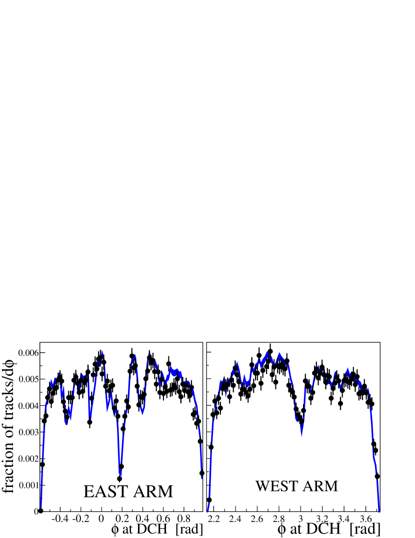
Figure 3: (Color online) Simulated (solid line) and real data (points) single electron distributions in the $\phi$ coordinate of the drift chamber. Error bars correspond to statistical uncertainties.

The detector response to $J/\psi~{}$and $\psi^{\prime}~{}$dielectron decays was studied using the geant-3 based Monte Carlo simulation. Malfunctioning detector channels were removed from the detector simulation and from the real data analysis. The geometric acceptance of the detector Monte Carlo was compared to that for real data using simulated $\pi^{0}$ decays. The majority of the electrons found in real data come from $\pi^{0}$ Dalitz decays and photons which convert to electrons in the detector structure. The simulated electrons from $\pi^{0}$ decays were weighted in order to match the collision vertex and $p_{T}$ distributions observed in the data. Fig. 3 shows the simulated and real electron track distribution as a function of the azimuthal angle, $\phi$, measured at the DCH radius. The ratio between real and simulated track distributions ($f_{acc}(\phi_{DCH},z_{DCH})$) is used later to estimate the systematic uncertainty of the $J/\psi~{}$acceptance.

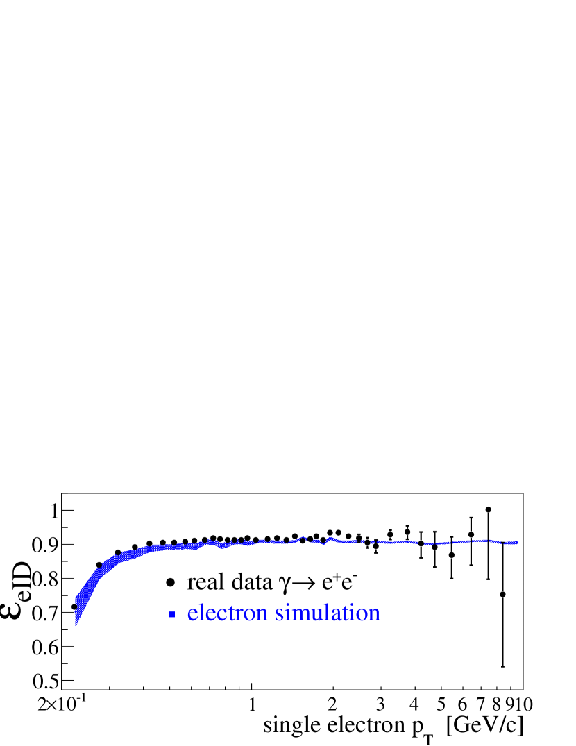
Figure 4: Single electron identification efficiency estimated using photon conversions from real data (points) and the electron simulation (shaded area).

The electron identification efficiency was estimated using $\gamma\rightarrow\mbox{$e^{+}e^{-}$~{}}$ conversions coming primarily from the beam pipe. These dielectrons, which do not originate from the event vertex, have a nonzero invariant mass and can be identified since their invariant mass exhibits a peak in the region below 30 MeV$/c^{2}$. Assuming all tracks in the peak above the combinatorial background are electrons, the electron identification efficiency was obtained from the fraction of dielectron conversions which survive the identification criteria applied to both electron and positron compared to the number of dielectron conversions obtained after requiring identification for only one electron or positron. The same procedure was repeated in the simulation. Fig. 4 shows the electron identification efficiency as a function of the $p_{T}$ of the electron in question. The difference in efficiency between simulation and data for electrons with $p_{T}>0.5$ GeV/$c~{}$was no larger than 0.8%, which translated to an overall type B uncertainty in the dielectron yield of 1.1% due to our understanding of the electron identification efficiency.

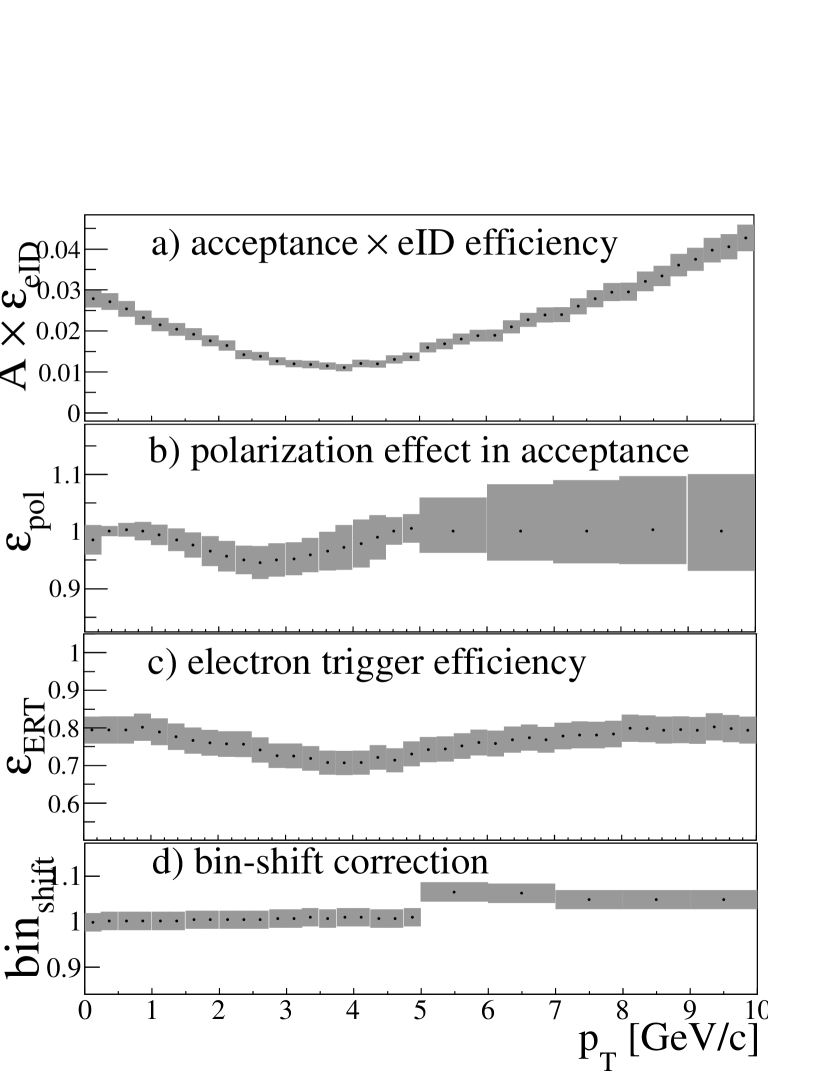
Figure 5: Transverse momentum dependence of the detector performance and correction factors for dielectron decays of $J/\psi~{}$mesons in $|y|<0.5$. Shaded bands are the uncertainties of the estimates as described in the text.

Simulated $J/\psi~{}$dielectron decays were generated with uniform $p_{T}$ and rapidity ($|y|<0.5$) and the measured vertex distribution. The fraction of the generated $J/\psi~{}$decays that were fully reconstructed corresponds to the acceptance $\times$ electron identification efficiency of the detector ($A\times\varepsilon_{eID}$) for $J/\psi~{}$dielectron decays with rapidity $|y|<0.5$ (Fig. 5-a). When each simulated electron decay was weighted according to $f_{acc}(\phi_{DCH},z_{DCH})$ given previously, the number of reconstructed $J/\psi~{}$decays was modified by 7.5%. This is essentially the variation in our acceptance calculation, when calculated using a data driven method as compared to simulation. We considered this deviation as a type B systematic uncertainty. The $A\times\varepsilon_{eID}$ for simulated $\psi^{\prime}~{}$dielectron decays in the same rapidity range was larger than that from the $J/\psi~{}$by between 5-20% because of its larger mass. The maximum difference occurs at $p_{T}\sim$2.5 GeV/$c~{}$.

The detector acceptance for charmonium also depends on the orientation of its electron decay with respect to the momentum direction of the parent particle, an outcome of charmonium polarization. The correction factor from polarization ($\varepsilon_{pol}$) was evaluated using a measurement of $J/\psi~{}$polarization Adare et al. (2010a) in $p$+$p$ collisions interpolated to the relevant transverse momentum. The uncertainty in $\varepsilon_{pol}$ due to the uncertainty in the polarization was assigned as a type B systematic uncertainty. In the $p_{T}$ region where there is no polarization measurement ($p_{T}>5$ GeV/$c~{}$for $J/\psi~{}$and all $p_{T}$ for $\psi^{\prime}~{}$) the one standard deviation uncertainty was calculated assuming the $J/\psi~{}$polarization in this region can be anything between -1 and 1. Fig. 5-b shows the $p_{T}$ dependence of $\varepsilon_{pol}$.

The trigger (ERT) performance was studied using single electrons. We used a MB data sample to measure the $p_{T}$ dependent fraction of electron candidates that fired the ERT in each of the EMCal sectors. These fractions were then used in simulation to estimate the $J/\psi~{}$efficiency of the ERT trigger ($\varepsilon_{ERT}$). This process was repeated for each change in the ERT operational conditions, such as a change in the energy threshold, or a significant modification in the number of EMCal or RICH sectors included in the ERT trigger. Fig. 5-c shows the $p_{T}$ dependence of $\varepsilon_{ERT}$, weighted by the luminosity accumulated in each ERT period. When the single electron ERT efficiency of each EMCal sector was varied within its statistical uncertainty, a one standard deviation change of 4.5% in $\varepsilon_{ERT}$ was observed. This deviation is shown in Fig. 5-c as the shaded band and is assigned as a type B systematic uncertainty for the $J/\psi~{}$and $\psi^{\prime}~{}$yields. No significant change in $\varepsilon_{ERT}$ was observed if one used the $\psi^{\prime}~{}$in the simulations.

A final correction ($bin_{shift}$) was made for the dominance of the yield in the lower end of each $p_{T}$ bin (Fig. 5-d). In addition, a correction of up to 2% was made to account for bin-by-bin smearing effects due to finite momentum resolution($bin_{smear}$).

III.3 Cross section results

The $J/\psi~{}$and $\psi^{\prime}~{}$dilepton differential cross section for each $p_{T}$ bin is calculated by

$$\frac{B_{ll}^{\psi}}{2\pi p_{T}}\frac{d^{2}\sigma_{\psi}}{dydp_{T}} = B_{ll}^{\psi}\frac{1}{2\pi p_{T}}\frac{d^{2}N/dydp_{T}}{\varepsilon_{inel.}\int\mathcal{L}dt}$$ (6)

$$\frac{d^{2}N}{dp_{T}dy} = \frac{N_{\psi}}{\Delta y\Delta p_{T}A\varepsilon},$$

where $B_{ll}^{\psi}$ is the branching ratio of the charmonium states into dileptons and $\varepsilon=\varepsilon_{eID}\varepsilon_{ERT}\varepsilon_{pol}\varepsilon_{mass}bin_{shift}bin_{smear}$.

All systematic uncertainties described in the previous sections are listed and classified in Table 1. The quadratic sum of the correlated systematic uncertainties (type B) is between 10% and 13% of the measured $J/\psi~{}$yield and between 12% and 22% of the measured $\psi^{\prime}~{}$yield, depending on $p_{T}$ .

Table 1: List of the systematic uncertainties relative to the $J/\psi~{}$and $\psi^{\prime}~{}$dielectron yields. Ranges indicate $p_{T}$ dependence.

description	contribution	type
fraction of $J/\psi~{}$in the mass cut	0.4%	A
fraction of $\psi^{\prime}~{}$in the mass cut	3-13%	A
acceptance	7.5%	B
eID efficiency	1.1%	B
mass cut efficiency for $J/\psi~{}$	1.0%	B
mass cut efficiency for $\psi^{\prime}~{}$	2.0%	B
heavy flavor MC used in fit for $J/\psi~{}$	0.5-1.1%	B
heavy flavor MC used in fit for $\psi^{\prime}~{}$	4.8-10%	B
up-in-down bin correction	3%	B
momentum smear effect	1.5%	B
$p_{T}$ , $y$ and vertex input in $\psi$ MC	2.0%	B
$J/\psi~{}$polarization bias in acceptance	0-10%	B
$\psi^{\prime}~{}$polarization bias in acceptance	4-17%	B
ERT efficiency	4.5%	B
luminosity	10%	C

The $p_{T}$ dependencies of the measured $J/\psi~{}$and $\psi^{\prime}~{}$yields are shown in Fig. 6(top) and Tables 7, 8. The bars correspond to the quadratic sum of all type A and statistical uncertainties. Boxes represent the quadratic sum of the type B uncertainties. There is a global uncertainty (type C) of 10%.

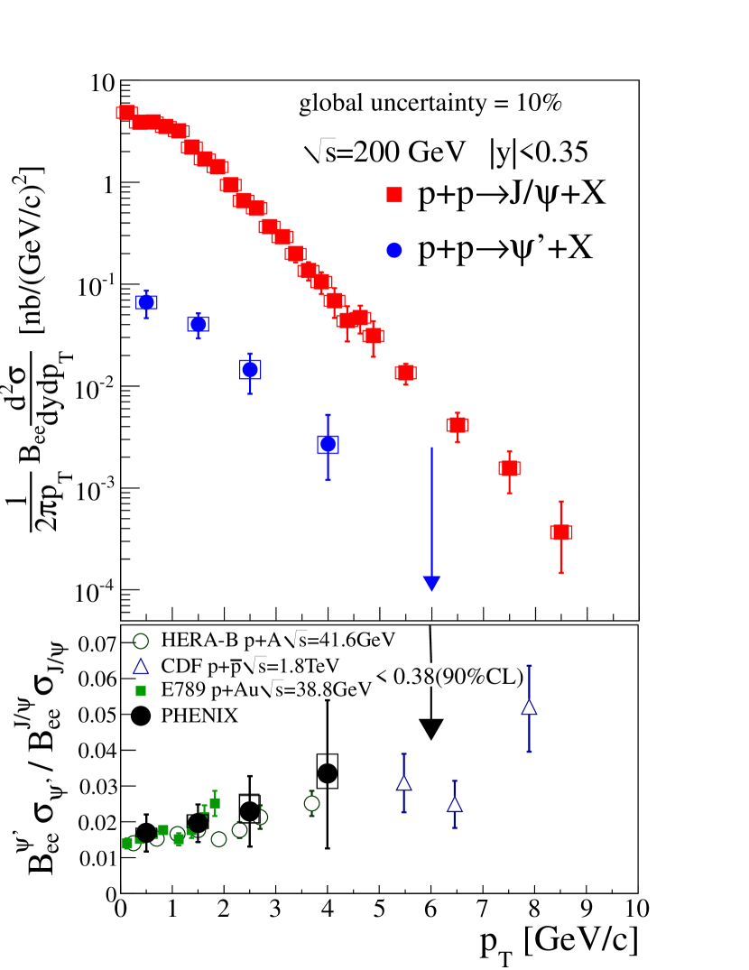
Figure 6: Transverse momentum dependence of $J/\psi~{}$and $\psi^{\prime}~{}$yields in $|y|<0.35$ (top). $\psi^{\prime}~{}$/($J/\psi~{}$) ratio together with ratios obtained in other experiments (bottom). Error bars reflect statistical and type A uncertainties while boxes reflect the quadratic sum of type B uncertainties).

The $p_{T}$ integrated $J/\psi~{}$cross section was calculated for three rapidity ranges using

$$B_{ll}\frac{d\sigma}{dy}=\sum_{p_{T}}B_{ll}\frac{d^{2}\sigma}{dp_{T}dy}\Delta p_{T}$$ (7)

where $B_{ll}d^{2}\sigma/dp_{T}dy$ is obtained from (6) using $A\varepsilon_{eID}$, $\varepsilon_{ERT}$ and $\varepsilon_{pol}$ recalculated for each of the three rapidity bins. The results are listed in Table 9 and shown in Fig. 18.

III.4 $\psi^{\prime}$/($J/\psi~{}$) yield ratio and fraction of $J/\psi~{}$yield coming from $\psi^{\prime}~{}$decays.

The decay of $\psi^{\prime}~{}$to $J/\psi~{}$cannot be measured in the current detector configuration. However, we can calculate the fraction of $J/\psi~{}$coming from $\psi^{\prime}~{}$decays $\left(F_{\psi^{\prime}}^{J/\psi}\right)$ using the ratio between the $\psi^{\prime}~{}$and $J/\psi~{}$cross sections and the $\psi^{\prime}~{}$branching ratio to $J/\psi~{}$($B_{J/\psi}^{\psi^{\prime}}=(58.7\pm 0.8)$% Amsler et al. (2008 and 2009 partial update for the 2010 edition)).

$$F_{\psi^{\prime}}^{J/\psi} = \frac{B_{J/\psi}^{\psi^{\prime}}\sigma_{\psi^{\prime}}}{\sigma_{J/\psi}}.$$ (8)

We start from the ratio between the $\psi^{\prime}~{}$and the $J/\psi~{}$dielectron counts $R_{J/\psi}^{\psi^{\prime}}$. Its joint probability distribution is calculated from the expected Poisson probability distributions (Eq. 4) $P_{\psi^{\prime}}(s_{\psi^{\prime}})$ and $P_{J/\psi}(s_{J/\psi})$ for the dielectron counts in the $\psi^{\prime}~{}$and $J/\psi~{}$mass ranges respectively, and the corresponding values $f_{\psi^{\prime}}$ and $f_{J/\psi^{\prime}}$ which account for the fraction of $\psi^{\prime}~{}$and $J/\psi~{}$contributions in the chosen dielectron mass ranges:

$$P\left(R_{J/\psi}^{\psi^{\prime}}\right)=\frac{P_{\psi^{\prime}}(s_{\psi^{\prime}})f_{\psi^{\prime}}}{P_{J/\psi}(s_{J/\psi})f_{J/\psi}}.$$ (9)

The $\psi^{\prime}$/($J/\psi~{}$) dielectron cross section ratio is thus determined as follows where the different correction factors for $\psi^{\prime}~{}$and $J/\psi~{}$must be taken into account.

$$\frac{B_{e^{+}e^{-}}^{\psi^{\prime}}\sigma_{\psi^{\prime}}}{B_{e^{+}e^{-}}^{J/\psi}\sigma_{J/\psi}}=\left<R_{J/\psi}^{\psi^{\prime}}\right>\frac{(A\varepsilon_{eID})^{J/\psi}\varepsilon_{ERT}^{J/\psi}\varepsilon_{mass}^{J/\psi}\varepsilon_{pol}^{J/\psi}}{(A\varepsilon_{eID})^{\psi^{\prime}}\varepsilon_{ERT}^{\psi^{\prime}}\varepsilon_{mass}^{\psi^{\prime}}\varepsilon_{pol}^{\psi^{\prime}}}.$$ (10)

Type A uncertainties are propagated for $f_{\psi^{\prime}}$ and $f_{J/\psi^{\prime}}$ while common relative type B uncertainties that are correlated for $J/\psi~{}$and $\psi^{\prime}~{}$cancel. The remaining uncertainty in the ratio comes from the quadratic difference between type B uncertainties which are different for the $J/\psi~{}$and $\psi^{\prime}$. The $\psi^{\prime}$/($J/\psi~{}$) dielectron cross section ratio is shown in the bottom panel of Fig. 6. The numbers are listed in Table 10.

Using the branching ratios, $B_{e^{+}e^{-}}^{\psi^{\prime}}=(0.765\pm 0.017)\%$ and $B_{e^{+}e^{-}}^{J/\psi}=(5.94\pm 0.06)\%$ Amsler et al. (2008 and 2009 partial update for the 2010 edition) in (8) gives

$$F_{\psi^{\prime}}^{J/\psi}=(9.6\pm 2.4)\%.$$ (11)

IV Radiative decay of $\chi_{c}$ 

The decay channel $\mbox{$\chi_{c}$~{}}\rightarrow\mbox{$J/\psi~{}$}+\gamma\rightarrow\mbox{$e^{+}e^{-}$~{}}+\gamma$ is fully reconstructed in the central arms and is used to directly measure the feed-down fraction of $\chi_{c}$ decays in the inclusive $J/\psi~{}$yield ($F_{\chi_{c}}^{J/\psi}$). This measurement is particularly challenging since the photon is typically of very low energy. The data sample used in this measurement and the $\gamma$ identification procedure is described in Section IV.1. The detector performance for the measurement of photon decays of the $\chi_{c}$ is discussed in Section IV.2. The composition of all combinatorial and correlated backgrounds for the $\chi_{c}$ signal in the $\mbox{$e^{+}e^{-}$~{}}\gamma$ mass distribution is detailed in Section IV.3. Section IV.4 presents the final feed-down fraction calculation and a summary of all uncertainties.

IV.1 Selection of $\mbox{$\chi_{c}$~{}}\rightarrow\mbox{$J/\psi~{}$}+\gamma$ decays

The analysis of the radiative decay of the $\chi_{c}$ requires the identification of photons with energy ($E_{\gamma}$) as low as 300 MeV, the lower limit of the energy we allow in this analysis. Photons were identified as energy clusters in the EMCal whose profile is consistent with an electromagnetic shower. This profile is based on the response of the EMCal to electron beam tests performed before the EMCal installation Aphecetche et al. (2003). Energy clusters that were closer than four standard deviations (of the energy cluster position resolution) to reconstructed charged tracks were rejected, in order to remove electron and misidentified hadron contributions. Electrons from photon conversions in detector material which were not reconstructed by the tracking system were removed by requiring energy clusters to be further than four standard deviations from hits in the Pad Chamber (PC) located in front of the EMCal.

The invariant mass of $e^{+}e^{-}+\gamma$ is formed using $e^{+}e^{-}$ pairs in a tight $J/\psi~{}$mass region of $2.9<M_{e^{+}e^{-}}[\mbox{GeV/$c^{2}~{}$}]<3.3$, avoiding the region where photons produced by Bremsstrahlung radiation can become an additional background in the 300 MeV energy region. The sample contains $N_{J/\psi}=$2456 $\pm$ 51 $e^{+}e^{-}$ pairs from $J/\psi~{}$decays, after removing combinatorial and correlated background as done previously. The $e^{+}e^{-}\gamma$ mass distribution is plotted in Fig. 12 (top), where we require E${}_{\gamma}>$300 MeV. The mass of $\mbox{$e^{+}e^{-}$~{}}\gamma$ minus the mass of the measured $e^{+}e^{-}$ pair is plotted in order to cancel the effect of the mass resolution in the $e^{+}e^{-}$ pair. The remaining resolution in the subtracted mass distribution is from the energy resolution of the measured photon.

IV.2 Detector performance for $\chi_{c}$ radiative decay

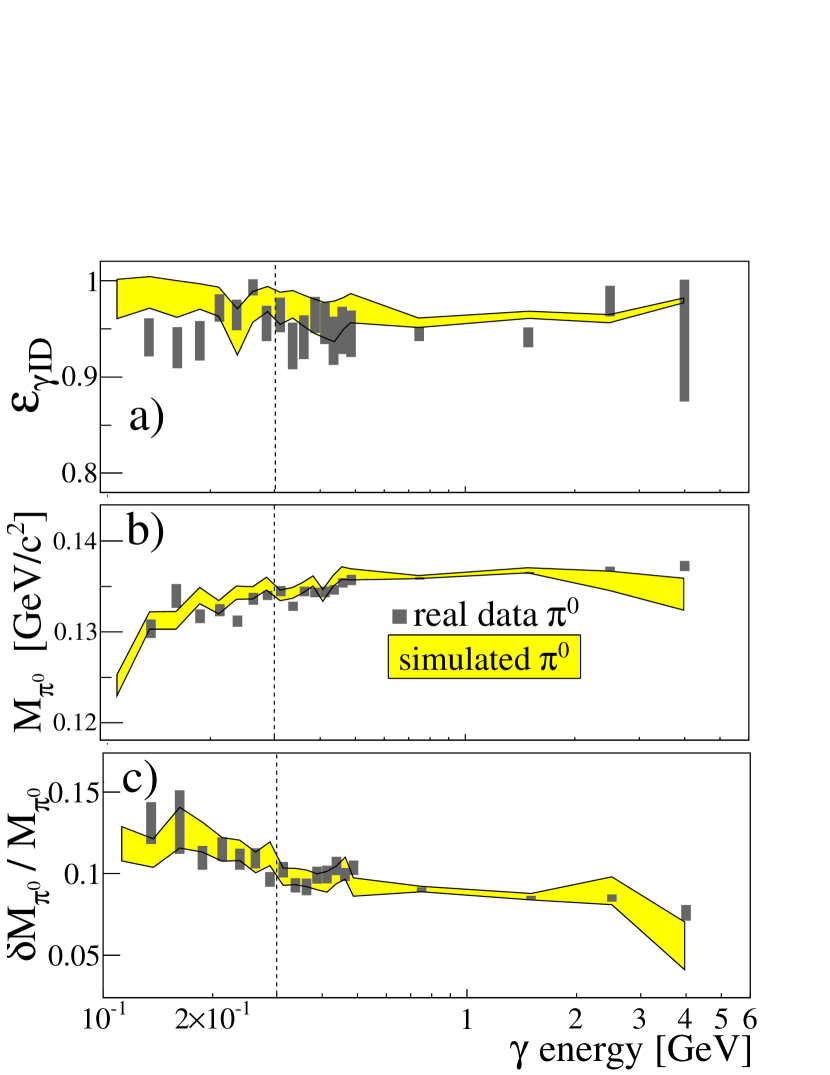
Figure 7: (Color online)Study of the $\pi^{0}$ detection performance using both the measured $\gamma$ energy in real data (boxes) and detector MC (shaded band). (a) $\gamma$ identification efficiency, (b) $\pi^{0}$ mass peak position, (c) $\pi^{0}$ mass resolution. The vertical dashed line represents the minimum $\gamma$ energy required in the $\chi_{c}$ analysis. Uncertainties are from the $\pi^{0}$ fit parameters in simulated and real data.

The resolution of the mass distribution $M_{e^{+}e^{-}\gamma}-M_{e^{+}e^{-}}$ is dominated by the photon energy resolution of the EMCal. Most photons from $\chi_{c}$ decays have energy close to the lower limit of the EMCal sensitivity. The behavior of the calorimeter was studied by using a clean sample of $\pi^{0}\rightarrow\gamma\gamma$ decays in real data and in the simulations. Pairs of clusters were formed where the invariant mass of the pair was required to be consistent with a $\pi^{0}$. Only one of the clusters was required to pass electromagnetic shower requirements. The photon identification efficiency was obtained assuming the other cluster of the pair was a photon. This was done on a statistical basis by subtracting a mixed event background to account for the small contamination from random clusters under the $\pi^{0}$ peak. Fig. 7-a shows the energy dependence of the photon identification efficiency ($\varepsilon_{\gamma ID}$) obtained using real and simulated $\pi^{0}$s. The simulation gives an efficiency 2.3% larger than that found in real data. This difference was assigned as a type B systematic uncertainty in $\varepsilon_{\gamma ID}$.

The central value of the $\pi^{0}$ mass peak decreases slightly as the photon energy approaches the lower limit of the calorimeter sensitivity. This behavior is caused by zero suppression during data acquisition and the energy cluster recognition algorithm. These effects are correctly reproduced in simulation as can be seen in Fig. 7-b. The $\gamma$ energy resolution ($\delta E_{\gamma}/E_{\gamma}$) was uniformly degraded by 4.7% in the simulation in order to match the mass resolution ($\delta M/M$) of the $\pi^{0}$ peaks observed in real data (Fig. 7-c).

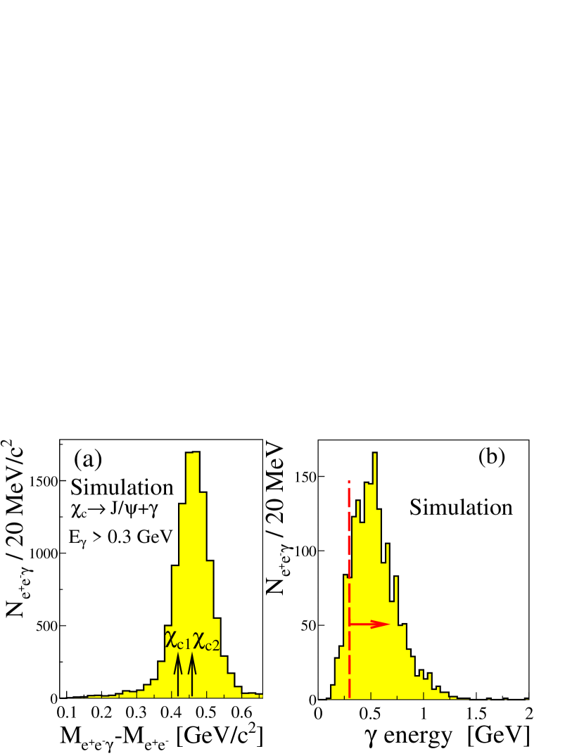
Figure 8: (Color online) Mass (a) and $\gamma$ energy (b) distributions of $\mbox{$e^{+}e^{-}$~{}}\gamma$ decays from $\chi_{c1}$ and $\chi_{c2}$ decays obtained from pythia + detector simulation. The dashed line in (b) represents the $\gamma$ energy cut applied in this analysis.

$\chi_{c1}$ and $\chi_{c2}$ states were generated using gluon+gluon scattering in pythia with the CTEQ6M PDF, requiring that the $J/\psi~{}$be in the rapidity range $|y|<0.5$. The $\chi_{c0}$ is not considered in the simulation because of its small branching ratio to $J/\psi~{}$of (1.14 $\pm$ 0.08)% Amsler et al. (2008 and 2009 partial update for the 2010 edition). Fig. 8 shows the mass and $\gamma$ energy distribution of $\mbox{$e^{+}e^{-}$~{}}\gamma$ decays of simulated $\chi_{c}$. The conditional acceptance of $\gamma$ from $\chi_{c}$ is plotted as a function of the $J/\psi~{}$momentum in Fig. 9. The detector geometric acceptance of the $\chi_{c}$ can be affected by its polarization and the polarization of the decay $J/\psi~{}$. There is no measurement of the $\chi_{c}$ polarization. Simulation studies found the overall acceptance is modified by at most 5.6% if the $\chi_{c}$ is totally transversely polarized. This possible modification was included in the acceptance type B systematic uncertainty.

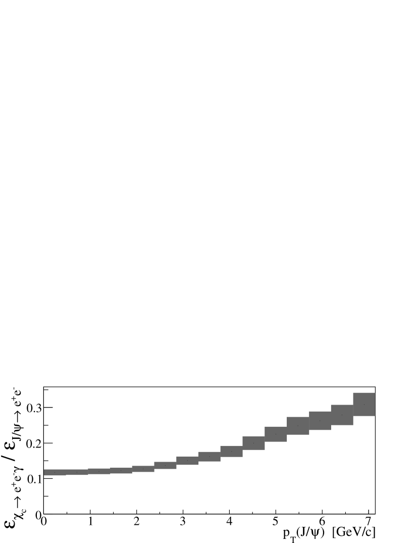
Figure 9: Conditional acceptance and efficiency of the $\chi_{c}$ decay $\gamma$ as a function of the $J/\psi~{}$transverse momentum. The height of the boxes corresponds to the type B systematic uncertainty due to the lack of knowledge of the polarization and the photon identification efficiency.

IV.3 Composition of the $\mbox{$e^{+}e^{-}$~{}}+\gamma$ sample.

In addition to the $\chi_{c}$ signal, the observed $\mbox{$e^{+}e^{-}$~{}}+\gamma$ sample is composed of combinatorial background, mostly coming from uncorrelated $\pi^{0}$ decays present in events where a $J/\psi~{}$is detected, and by photonic sources correlated to the $J/\psi~{}$which will be discussed later.

The combinatorial background from random $e^{+}e^{-}$ pairs (i.e. the combinatorial background to the $J/\psi~{}$in the $\chi_{c}$ decay) is well described by the sum of $e^{+}e^{+}\gamma$ and $e^{-}e^{-}\gamma$ mass distributions. This sum was normalized by the geometrical average of the two components, and subtracted from the $\mbox{$e^{+}e^{-}$~{}}\gamma$ mass spectrum. The mass distribution of random $(\mbox{$e^{+}e^{-}$~{}})+\gamma$ combinations (i.e. essentially random $J/\psi~{}$+$\gamma$ pairs) was obtained using the invariant mass distribution of $e^{+}e^{-}$ pairs from one event and photons another. In order to obtain the combinatorial background as realistically as possible, events used to form the $e^{+}e^{-}$ and $\gamma$ combination were required to have event vertices within 3 cm (2$\sigma$ of the vertex position resolution) of each other.

The sources of correlated background include internal and external (Bremsstrahlung) radiative decays of $J/\psi~{}$, i.e. $\mbox{$J/\psi$}\rightarrow\mbox{$e^{+}e^{-}$~{}}\gamma$, $\pi^{0}$s produced in jets containing $J/\psi~{}$, $\mbox{$\psi^{\prime}$}\rightarrow\mbox{$J/\psi~{}$}+$ neutral mesons, $B^{0}\rightarrow\mbox{$J/\psi~{}$}+$ X where X or its decays includes a $\gamma$. Another possibility is that a $J/\psi~{}$could be produced together with a high energy photonSridhar (1993). Recent studies also suggest an important contribution from $gg\rightarrow\mbox{$J/\psi~{}$}+\gamma+gg$ in NNLO calculations at $\sqrt{s}=$14 TeV Lansberg (2009b). No estimate was made for $\sqrt{s}=$ 200 GeV at the time of this writing. These sources will be considered in the next few paragraphs.

Photons produced by Bremsstrahlung radiation in the detector structure are very close to their associated electron and are rejected by the criteria that removes electrons in the $\gamma$ identification. The minimum dielectron mass cut of 2.9 GeV/$c^{2}~{}$also removes radiative $J/\psi~{}$decays with $E_{\gamma}>200$ MeV, i.e. those in the energy range of the photons used in this analysis.

Collisions containing primary $J/\psi~{}$mesons produced by gluon+gluon scattering (the dominant source) were simulated using pythia in order to understand the electron radiation and jet contributions. Only the $e^{+}e^{-}$ and the radiative $\mbox{$e^{+}e^{-}$~{}}\gamma$ decay channels were allowed. All final state particles with momentum larger than 100 MeV and $|\eta|<0.5$ were reconstructed. $J/\psi~{}$ and $\gamma$ identification criteria were the same as used in the analysis of real data. The $e^{+}e^{-}\gamma$ distribution obtained from this simulation is completely accounted for by combinatorial background from mixed events (Fig. 10(a)), leaving little room for contributions from possible jets containing $J/\psi~{}$, radiative decays or electron radiation when crossing the detector support.

Using the data, a check was done for possible missing correlated radiation backgrounds that might have been missing in the simulation. The invariant $e^{+}e^{-}\gamma$ mass distribution was formed in which we required $M_{e^{+}e^{-}}[\mbox{GeV/$c^{2}~{}$}]<$2.9. The $\chi_{c}$ contribution is small in this region and the correlated signal should be mainly from other sources, e.g. $J/\psi~{}$internal and external radiation. The data unlike the simulation shows a correlated background after combinatorial background subtraction (Fig. 10(b)). The line shape of this mass distribution can be described by a Gaussian distribution, Landau distribution, or a simulated $\mbox{$\psi^{\prime}~{}$}\rightarrow\mbox{$J/\psi~{}$}+\gamma$ shape. Its source could be the $gg\rightarrow\mbox{$J/\psi~{}$}+\gamma+gg$ process mentioned previously, but we simply take this as a background which must be included in the fit to the $\chi_{c}$ mass distribution. The position of the peak is set by the minimum photon energy cut of 300 MeV, while the width is set by energy spectrum of the source and more importantly by the smearing effect caused by the fact that the spectrum is a difference of two invariant mass calculations. These results will be used later when fitting the $\mbox{$e^{+}e^{-}$~{}}\gamma$ invariant mass distribution.

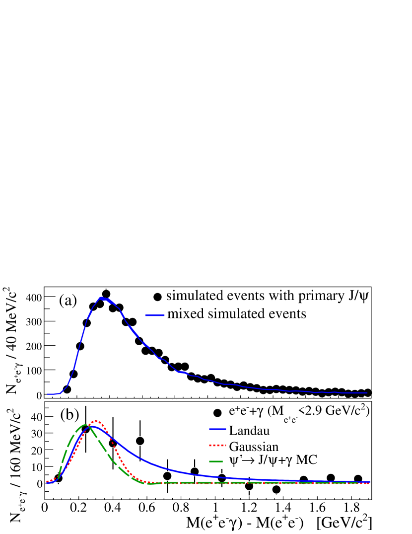
Figure 10: (Color online) (a) Simulated $e^{+}e^{-}+\gamma$ invariant mass distribution from pythia events containing primary $J/\psi~{}$decays. The line is the combinatorial background obtained using simulated mixed events from the same sample (top). (b) The $e^{+}e^{-}\gamma$ mass distribution in the data, after combinatorial background subtraction, where $M_{e^{+}e^{-}}[\mbox{GeV/$c^{2}~{}$}]<$2.9. The lines are empirical fits as explained in the text. Note that the simulated $\mbox{$\psi^{\prime}~{}$}\rightarrow\mbox{$J/\psi~{}$}+\gamma$ shape is arbitrarily normalized.

In section III.4 we reported that (9.6 $\pm$ 2.4)% of the $J/\psi~{}$counts in our sample come from $\psi^{\prime}~{}$decays. (41.4 $\pm$ 0.9)% of these decays contain a neutral meson that decays into photonsAmsler et al. (2008 and 2009 partial update for the 2010 edition), namely $\mbox{$\psi^{\prime}~{}$}\rightarrow\mbox{$J/\psi~{}$}+\pi^{0}\pi^{0}$, $\mbox{$\psi^{\prime}~{}$}\rightarrow\mbox{$J/\psi~{}$}+\pi^{0}$ and $\mbox{$\psi^{\prime}~{}$}\rightarrow\mbox{$J/\psi~{}$}+\eta$. We will refer to these decay channels collectively as $\mbox{$\psi^{\prime}~{}$}\rightarrow\mbox{$J/\psi~{}$}+n\gamma$. Simulations show that most of the decays into neutral mesons are either not detected in the central arm acceptance or are rejected by the $\gamma$ energy cut, leaving an estimated 6-20 counts in the low mass distribution of $\mbox{$e^{+}e^{-}$~{}}\gamma$ (Fig. 11). Contributions from $\mbox{$\psi^{\prime}~{}$}\rightarrow\gamma+\chi_{c}\rightarrow 2\gamma+\mbox{$J/\psi~{}$}$ decays are expected to be no larger than three counts.

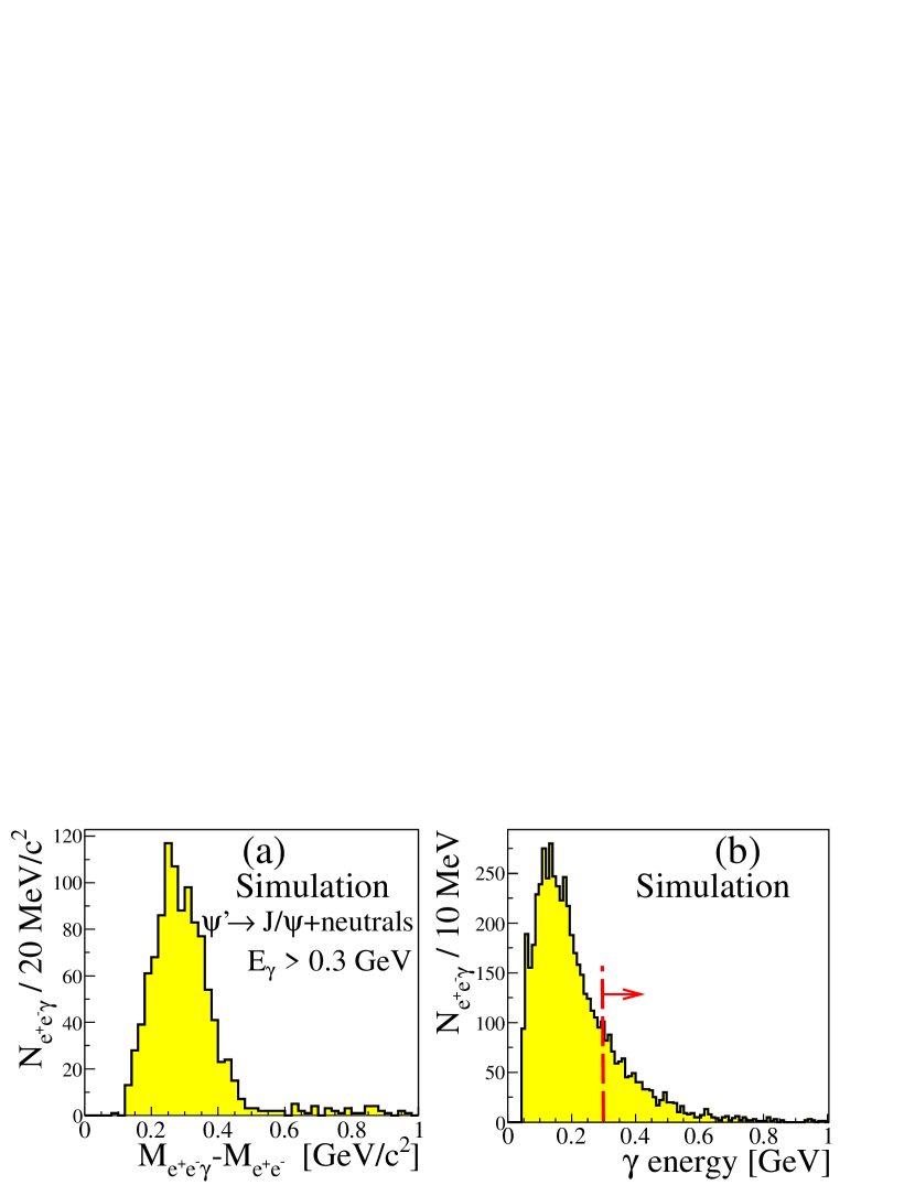
Figure 11: (Color online) Mass (a) and $\gamma$ energy (b) distributions of $\mbox{$\psi^{\prime}~{}$}\rightarrow\mbox{$J/\psi~{}$}+$neutrals $\rightarrow\mbox{$e^{+}e^{-}$~{}}\gamma$ obtained from simulations. Dashed lines in panel (b) represents the photon energy cut applied in this analysis. Appropriate scaling indicates that such events contribute between 6 and 20 counts to the correlated $\mbox{$e^{+}e^{-}$~{}}\gamma$ distribution.

The contribution from $B$ decays in the $\mbox{$e^{+}e^{-}$~{}}\gamma$ sample was calculated using the bottom cross section measured by PHENIX Adare et al. (2009a). The contribution of $B$ decays to $J/\psi~{}$plus at least one photon is less than 3 counts in the entire $e^{+}e^{-}\gamma$ sample.

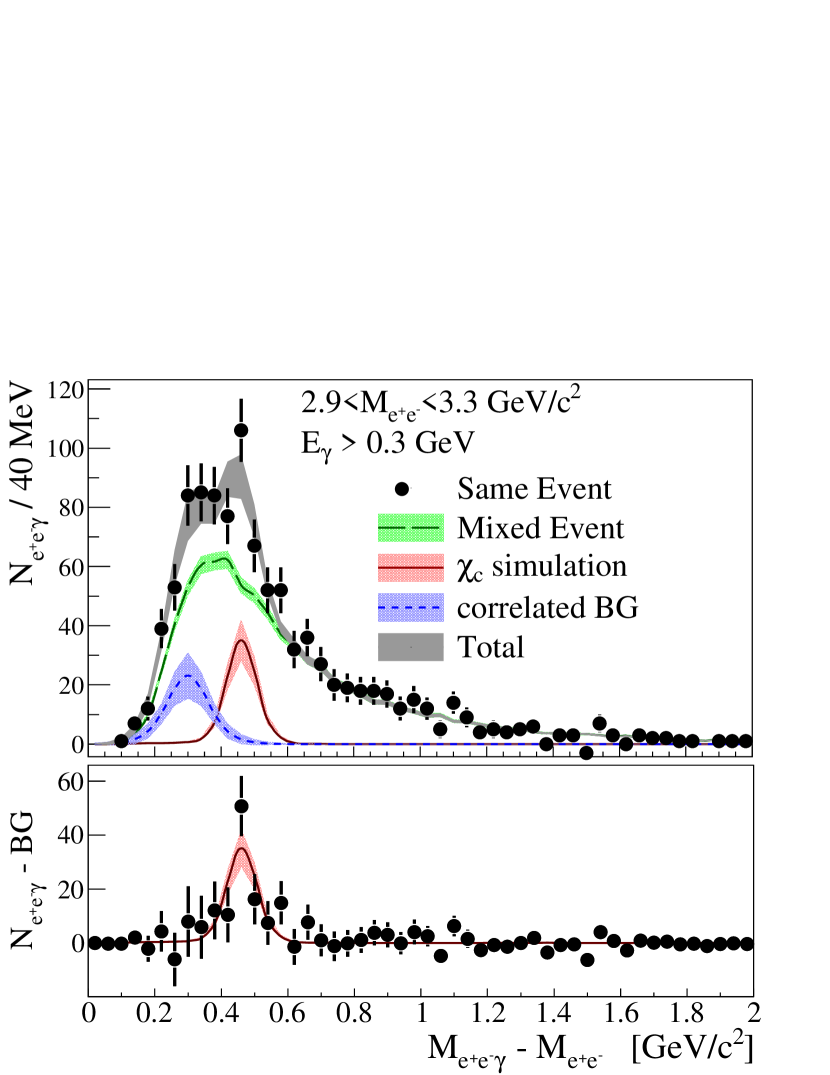
Figure 12: (Color online) Top plot: $e^{+}e^{-}\gamma$ invariant mass distribution where the dielectron is required to have an invariant mass within $J/\psi~{}$mass region. The like-sign dielectron distribution is subtracted as described in the text. Bands represent the contributions from various sources: solid line - $\chi_{c}$ signal; long dashed line - mixed event uncorrelated background; short dashed line - correlated background as described in the text. The correlated background was fit to a Gaussian for this plot. The widths of the bands reflects the 1$\sigma$ variations in the fit. The bottom plot is the $\chi_{c}$ signal after subtraction of the backgrounds.

The number of $\chi_{c}$ decays was obtained by fitting the background and the simulated $\chi_{c}$ line shapes to the measured $e^{+}e^{-}\gamma$ mass distribution (Fig. 12). The background includes two sources: the mixed event background from random $e^{+}e^{-}$ + $\gamma$ combinations, and the correlated background discussed previously. The correlated background was fit to a Gaussian and a Landau distribution where the maximum of the correlated background was set by the photon energy cut. In addition, the $\mbox{$\psi^{\prime}~{}$}\rightarrow\mbox{$J/\psi~{}$}+n\gamma$ background was used as a third shape in estimating the systematic error. However, it must be emphasized that this background cannot explain the magnitude of the correlated background. The variations introduced by using the three distributions contribute to the type B systematic errors. The fitting parameters included the combinatorial background normalization, the amplitude of the correlated background and, when used, the width of the Gaussian and Landau shapes (the $\mbox{$\psi^{\prime}~{}$}\rightarrow\mbox{$J/\psi~{}$}+n\gamma$ shape was fixed from simulations), and the normalization of the simulated $\chi_{c}$ mass distribution. The fitted $\chi_{c}$ mass spectrum returned an average value 96 $\pm$ 24 counts in the $\chi_{c}$ mass range $M_{e^{+}e^{-}\gamma}-M_{e^{+}e^{-}}\in[0.3,0.6]$ GeV/$c^{2}~{}$when fitting the three different line shapes to the correlated background. The signal/background, including the correlated background, was 1/5. The number of $\chi_{c}$ counts changed by $\pm$ 4.6% when using different line shapes for the correlated background (Gaussian, Landau or $\mbox{$\psi^{\prime}~{}$}\rightarrow\mbox{$J/\psi~{}$}+n\gamma$ shapes).

IV.4 Feed-down fraction result

The fraction of $J/\psi~{}$counts coming from $\chi_{c}$ decays is

$$F_{\mbox{$\chi_{c}$~{}}}^{J/\psi}=\frac{N_{\chi_{c}}}{N_{J/\psi}}\frac{1}{\left<\varepsilon_{\chi_{c}}/\varepsilon_{J/\psi}\right>}.$$ (12)

To find the mean conditional acceptance, $\left<\varepsilon_{\chi_{c}}/\varepsilon_{J/\psi}\right>$, the conditional acceptance shown in Fig. 9 must be convoluted with the $\chi_{c}$ $p_{T}$ distribution. An estimate of the $\chi_{c}$ $p_{T}$ distribution was obtained by fitting a two dimensional $e^{+}e^{-}\gamma$ mass vs. $p_{T}$ distribution to a $\chi_{c}$ signal plus backgrounds and extracting the number of $\chi_{c}$ counts in several $p_{T}$ bins. While the statistical errors are large, the dependence of the acceptance on the $p_{T}$ of the $\chi_{c}$ is mild, hence the error in the mean conditional acceptance is small. We obtain ($\varepsilon_{\chi_{c}}/\varepsilon_{J/\psi}$) = (12.0 $\pm$ 0.4) %.

Tests of the fitting procedure and the conditional acceptance calculation were performed using several different simulated data sets with varying amounts of $\chi_{c}$ signal, $J/\psi~{}$, and backgrounds. The feed-down observed after full analysis of the six sets of simulated events correctly returned the fraction of $\chi_{c}$ events with no significant bias. Variations in the minimum $E_{\gamma}$ criteria changed the measured feed-down in the simulation by 1.7%. This variation is taken into account in the uncertainties as a type B error introduced by the analysis procedure. When the photon energy resolution is changed in a manner consistent with the measured $\pi^{0}\rightarrow 2\gamma$ mass resolution, both the conditional acceptance and the $\chi_{c}$ counts returned from the fits change, leading to a variation of the feed-down fraction by 1.6%. The list of all systematic uncertainties is shown in Table 2.

Table 2: Summary of the type B systematic uncertainties in the $\chi_{c}$ feed-down fraction measurement. The total gives the sum of all errors in quadrature.

syst uncertainty	contribution	type
$\gamma$ ID	0.7%	B
energy resolution	1.6%	B
$\chi_{c}$ polarization	1.8%	B
correlated background line shape	1.5%	B
$J/\psi~{}$continuum	0.1%	B
fit procedure	1.7%	B
$\chi_{c}$ momentum dependence	1.1%	B
TOTAL	3.6 %

The final $\chi_{c}$ feed-down fraction using (12) is

$$F_{\chi_{c}}^{J/\psi}=32\pm 9\%$$ (13)

when taking the quadratic sum of the statistical and systematic uncertainties.

V $J/\psi~{}$analysis in the forward rapidity region

This section describes the analysis performed to obtain the inclusive $J/\psi~{}$dimuon yield at forward rapidity $1.2<|y|<2.4$. Section V.1 describes the $J/\psi~{}$signal extraction from the dimuon spectrum and related uncertainties. The response of the muon arm spectrometers to dimuon decays from the $J/\psi~{}$is described in section V.2. Finally, the $p_{T}$ and rapidity dependence of the $J/\psi~{}$differential cross section and a summary of systematic uncertainties is reported in section V.3.

V.1 $\mbox{$J/\psi~{}$}\rightarrow\mu^{+}\mu^{-}$ signal extraction

The dimuon invariant mass spectrum was obtained from the muon sample selected according to the criteria described in Sec. II. The MuID trigger condition is emulated offline. In order to make sure the real $J/\psi~{}$candidate fired the MuID trigger, at least one muon of the dimuon pair is required to match a road from the trigger emulator.

The decomposition of the dimuon background is very similar to that described in Sec. III.1 for dielectrons. The combinatorial background was estimated using the mass spectrum of random pairs formed by pairing opposite sign muon candidates from different events. The muons of the mixed pair are required to have vertices that differ by no more than 3 cm in the beam direction. The mixed event spectrum was normalized by the factor

$$\alpha=\frac{\sqrt{(N_{\mu^{+}\mu^{+}}^{\rm same})(N_{\mu^{-}\mu^{-}}^{\rm same})}}{\sqrt{(N_{\mu^{+}\mu^{+}}^{mixed})(N_{\mu^{-}\mu^{-}}^{mixed})}},$$ (14)

where $N_{\mu\mu}^{\rm same}$ and $N_{\mu\mu}^{mixed}$ are the number of pairs formed from two muons in the same or in mixed events, respectively. The mass spectrum of the dimuons in the $J/\psi~{}$mass region is shown in Fig. 13.

Figure 13: (Color online) Invariant mass distribution of dimuons in the $J/\psi~{}$mass region. The components of the spectrum are the combinatorial background estimated from a mixed-event technique, an acceptance modified (Fig. 14) two-Gaussian $J/\psi~{}$signal, and an acceptance modified exponential continuum (Eq. 15).

The components of the correlated dimuon spectrum are muons sharing the same $c\bar{c}$ or $b\bar{b}$ ancestor, dimuons from Drell-Yan and the $J/\psi~{}$and $\psi^{\prime}~{}$resonances. There is no clean mass discrimination between the $J/\psi~{}$and $\psi^{\prime}~{}$mass peaks in the muon arm spectrometers. However the $\psi^{\prime}~{}$contribution is expected to be negligible in the peak integral compared to other uncertainties. The correlated dimuon mass distribution can be represented by a function $F(M_{\mu\mu})$ including an exponential shape accounting for the continuum distribution, a double Gaussian which describes the line shape of $J/\psi~{}$in the Monte Carlo, and acceptance dependence:

$$\centering\frac{F(M_{\mu\mu})}{Acc\left(M_{\mu\mu}\right)}\@add@centering = A_{\psi}F_{\psi}(M_{\mu\mu})+A_{cont}e^{-\frac{M_{\mu\mu}}{b_{cont}}}$$ (15)

$$F_{\psi}(M_{\mu\mu}) = (1-f_{G2})G\left(M_{\mu\mu},M_{J/\psi},\sigma_{G1}\right)$$

$$+ f_{G2}G\left(M_{\mu\mu},M_{J/\psi}+\delta_{M},\sigma_{G2}\right)$$

$$G\left(M_{\mu\mu},M,\sigma\right) = \frac{1}{\sqrt{2\pi}\sigma}e^{-\frac{(M_{\mu\mu}-M)^{2}}{2\sigma^{2}}}$$

where $Acc\left(M_{\mu\mu}\right)$ is the mass dependence of the dimuon acceptance in the rapidity 1.2$<|y|<$2.4 estimated using dimuon simulation (Fig. 14), $A_{\psi}$ is the amplitude of the $J/\psi~{}$signal with mass $M_{J/\psi}$ composed of a Gaussian of width $\sigma_{G1}$ and a second Gaussian of width $\sigma_{G2}$ shifted by $\delta M$ in mass. $f_{G2}$ describes the fractional strength of the second Gaussian. The normalization of the continuum contribution is $A_{cont}$ and its exponential slope is $b_{cont}^{-1}$.

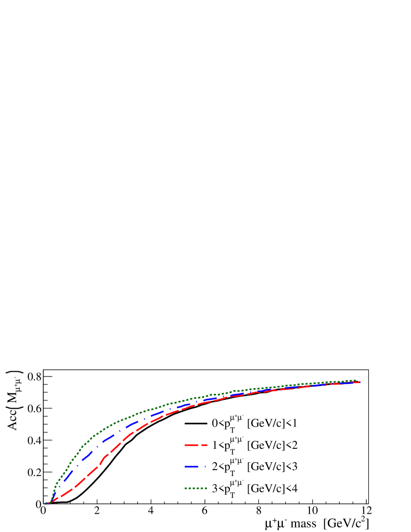
Figure 14: (Color online) Mass dependence of the dimuon geometric acceptance in the muon arm spectrometers.

The correlated mass distribution function $F\left(M_{\mu\mu}\right)$ was fit to the measured unlike-sign dimuon mass distribution for each $p_{T}$ and rapidity range using the maximum likelihood method. The combinatorial background, obtained from the normalized mixed event distribution, was also introduced in the fit with a fixed amplitude. The mass resolution obtained in the entire $J/\psi~{}$sample was $\sigma_{G1}/M_{J/\psi}=$4% ($\sigma_{G1}=125$ MeV). The fitting parameters which determine the line shape of the $J/\psi~{}$peak ($\sigma_{G1}$, $\sigma_{G2}$, $\delta_{M}$ and $f_{G2}$) obtained from the entire unbinned sample were fixed when performing fits for individual $p_{T}$ and rapidity bins. The $J/\psi~{}$mass, $M_{J/\psi}$, was allowed to vary by 10% of its nominal value (3.096 GeV/$c^{2}~{}$) in the fitting procedure, the $J/\psi~{}$and continuum amplitudes were constrained to avoid unphysical negative values, and the exponential slope was allowed to vary by 20% from a the value found in a fit to the entire (unbinned) sample. For the systematic uncertainty evaluation, $f_{G2}$ was changed by 25% up and down, the fit was performed in two mass ranges: 1.8 $<M_{\mu\mu}[\mbox{GeV/$c^{2}~{}$}]<$7.0 and 2.2$<M_{\mu\mu}[\mbox{GeV/$c^{2}~{}$}]<$6.0 and the combinatorial background normalization $\alpha$ was varied by $\pm$2%. Fig. 13 shows the fitted function and its components for the dimuon unlike-sign distribution for one of the rapidity bins. Two methods for counting the $J/\psi~{}$s were considered: 1) using the fitted amplitude $A_{\psi}$ directly, or 2) from direct counting of dimuon pairs in the mass region 2.6 $<M_{\mu^{+}\mu^{-}}[\mbox{GeV/$c^{2}~{}$}]<$ 3.6 with subtraction of the combinatorial background and exponential continuum underneath the peak in that same region. The standard deviations of the central values of the fits and of the signal extraction method variations are taken as type A signal extraction systematic uncertainties, since these variations are largely driven by statistical variations. The total number of $J/\psi~{}$counts was $16,612\pm 147^{\rm stat}\pm 112^{\rm syst}$ in the south muon arm and $16,669\pm 145^{\rm stat}\pm 115^{\rm syst}$ in the north muon arm.

V.2 Di-muon acceptance and efficiency studies

Figure 15: (Color online) Simulated (shaded area) and real data (bars) single muons distributed in the $\phi$ coordinate of the MuTr.

The response of the muon arm spectrometers to dimuons from $J/\psi~{}$ decays was studied using a tuned geant3-based simulation of the muon arms and an offline MuID trigger emulator. The MuID panel-by-panel efficiency used in these simulations was estimated from reconstructed roads in real data, or in cases with low statistics, from a calculation based on the operational history record for each channel. The MuID efficiency had a variation of 2% throughout the Run leading to a systematic uncertainty of 4% for the $J/\psi~{}$yield.

The charge distribution in each part of the MuTr observed in real data and the dead channels and their variation with time over the run were used to give an accurate description of the MuTr performance within the detector simulation. The azimuthal distribution of muon candidates in real data and simulated muons from $J/\psi~{}$decays using the pythia simulation are shown in Fig. 15. The $Z$ vertex distribution of simulated $J/\psi~{}$decays is the same as that observed in real data. The $p_{T}$ distribution in the MuTr obtained in simulation was also weighted according to that observed in the real data. The relatively small differences in the real and simulated $\phi$ distributions (Fig. 15) are thought to be due primarily to missing records for short periods of time in the dead HV channel records. These differences are estimated to change the $J/\psi~{}$dimuon yields by up to 6.4(4.0)% in north(south) arms. Run-by-run variations of the MuTr single muon yields are estimated to affect the final $J/\psi~{}$yields by an additional 2%.

The $J/\psi~{}$acceptance $\times$ efficiency ($A\varepsilon$) evaluation used a pythia simulation with several parton distributions as input to account for the unknown true rapidity dependence of the $J/\psi~{}$yield leading to variations of 4% in the final acceptance. Fig. 16 shows the overall $p_{T}$ dependence of $A\varepsilon$ for $J/\psi~{}$dimuon decays. The uncertainties related to the knowledge of the detector performance are point-to-point correlated between different $p_{T}$ and different rapidity bins. The uncertainty in the dimuon acceptance caused by lack of knowledge of the $J/\psi~{}$polarization was studied using the detector simulation. The first results in PHENIX at forward rapidity PPG121 (2010) indicate that the $J/\psi~{}$polarization is no larger than $\pm$0.5 for $p_{T}<$5 GeV/$c~{}$(in the Helicity frame). For this polarization variation, the simulations show one standard deviation variations between 2% and 11%, with the largest variation occurring for $p_{T}<$1 GeV/$c~{}$and $y\simeq$ 1.2. For $p_{T}>5$ GeV/$c~{}$, where there are no polarization measurements we consider polarizations anywhere between $\pm$1, and find variations no larger than 5%. These deviations are considered as type B uncertainties.

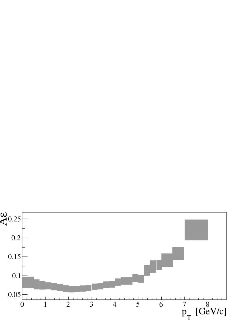
Figure 16: Transverse momentum dependence of the north and south average muon arms acceptance $\times$ efficiency for $J/\psi~{}$dimuon decays in $1.2<|y|<2.4$. Shaded bands are the uncertainties of the estimates described in the text.

V.3 $J/\psi~{}$dimuon cross section result

The differential cross section for each $p_{T}$ bin was calculated according to Eq. (6). The systematic uncertainties involved in this calculation are listed in Table 3.

Table 3: List of the systematic uncertainties in the $J/\psi~{}$dimuon yield measurement. Ranges indicate $p_{T}$ dependence.

description	relative uncertainty	type
signal extraction	1.8% - 35%	A
MuID efficiency	4%	B
MuTr acceptance	6.4%(north), 4.0%(south)	B
run-by-run fluctuation	2%	B
Monte Carlo $J/\psi~{}$input	4%	B
$J/\psi~{}$polarization	2% - 11%	B
luminosity	10%	C

The differential cross section was independently obtained in the north and south muon arm spectrometers and for the 2006 and 2008 Runs. The measurements agree in all data sets for all $p_{T}$ points within one sigma statistical and systematic uncertainties. The averaging of these four momentum spectra is done using a weight for each data set based on the uncertainties for each that are uncorrelated between data sets. By definition the statistical and type A uncertainties are uncorrelated and while the type C is correlated. The uncertainties in the MuTr efficiency and run-by-run variations are also uncorrelated between data sets. The MuID efficiency and the simulation input uncertainty are correlated between different spectrometer arms and run periods. Fig. 17 shows the resulting average differential cross section for dimuons from $J/\psi~{}$. The numbers are listed in Table 11.

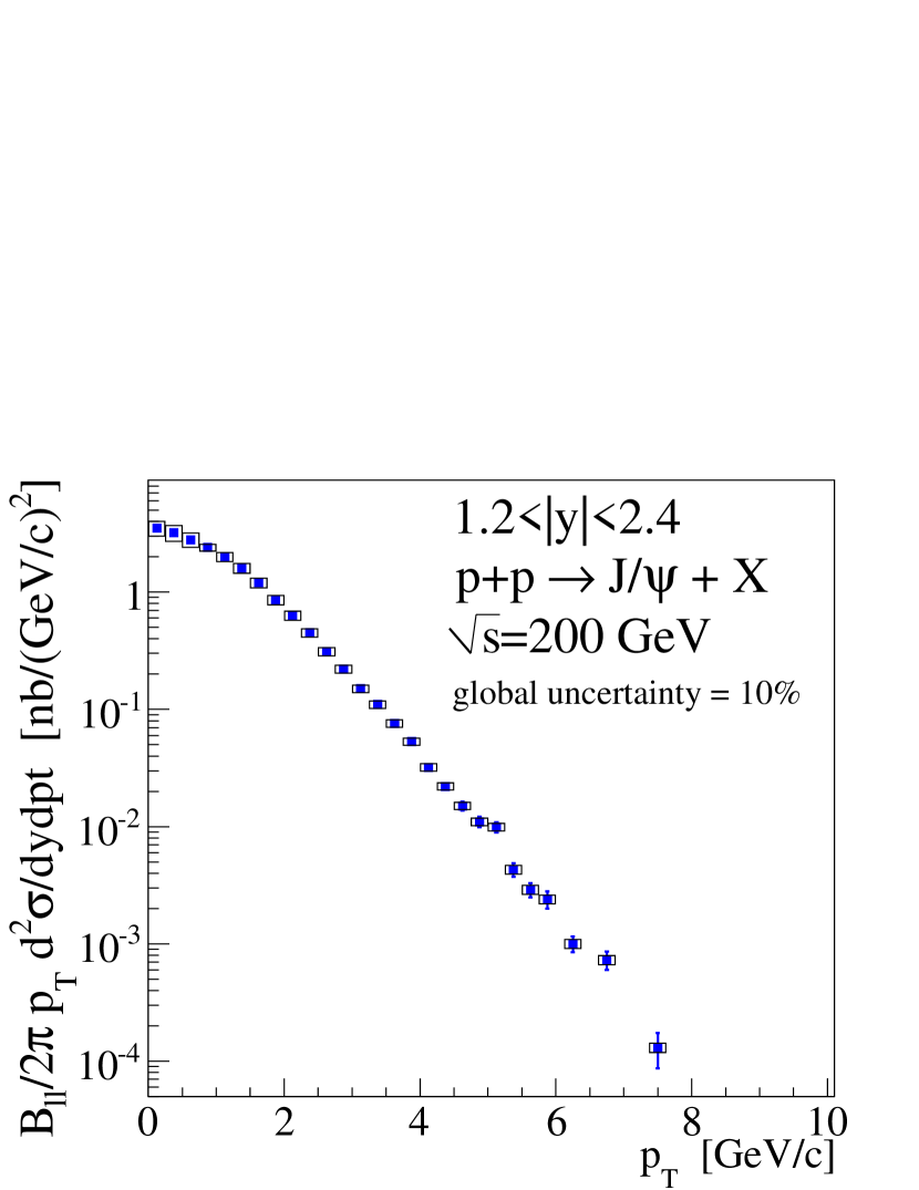
Figure 17: Transverse momentum dependence of the $J/\psi~{}$dimuon differential cross section obtained in the muon arms in 2006 and 2008 Runs.

The rapidity distribution was calculated as:

$$B_{\mu\mu}\frac{d\sigma}{dy}=\frac{N_{J/\psi}}{\Delta y\varepsilon_{inel.}\int\mathcal{L}dtA\varepsilon},$$ (16)

where the number of $J/\psi~{}$counts $N_{J/\psi}$ and the acceptance $\times$ efficiency estimates were performed for each rapidity bin. All these results are shown in Fig. 18 and the numerical results are listed in Table 9.

VI Results Discussion

This section presents a summary of the results reported in the previous sections and compares them with results obtained in other experiments as well as predictions from several different production mechanism calculations. The rapidity dependence of the $J/\psi~{}$yield is compared to models using various parton distribution functions (PDF) in Sec. VI.1. The total $J/\psi~{}$cross section is derived from the rapidity distribution and discussed in Sec. VI.2. The $J/\psi~{}$differential cross section dependence on $p_{T}$ is compared to empirical scaling laws observed at lower energies as well as different charmonium hadronization models in Sec. VI.3. The measured fraction of the $J/\psi~{}$yield coming from $\psi^{\prime}~{}$and $\chi_{c}$ decays is compared to other experiments in Sec. VI.4. The consequences of the results presented in this article on recent charmonium measurements in $p$(d)+A and A+A collisions is the subject of the Sec. VI.5.

The models used in our comparisons were described in Sec. I; namely, the Color Evaporation Model (CEM), the Color Singlet Model (CSM) and Non-relativistic QCD (NRQCD). The CEM used FONLL calculations for the charm cross section and CTEQ6M as the parton distribution functionFrawley et al. (2008); Vogt (2009). For the CSM comparison, we used the recent NLO calculation only for the direct $J/\psi~{}$yield at RHIC energy and PHENIX rapidity coverage Lansberg (2010). We used two NRQCD calculations in our comparisons. The calculation performed for the direct $J/\psi~{}$plus $\chi_{c}$ feed-down in Butenschön and Kniehl (2011) uses NLO diagrams for the color singlet and color octet states with a long range matrix element tuned from experimental hadroproduction Acosta et al. (2005) and photoproduction Adloff et al. (2002); Aaron et al. (2010) results. This calculation is only available for the differential $p_{T}$ dependent cross section. An older calculation, performed for the same direct $J/\psi~{}$plus $\chi_{c}$ feed-down with LO diagrams Cooper et al. (2004), also provides the rapidity dependence and total cross sections for different PDFs. No similar attempt has been made with the new calculations. The differential $p_{T}$ dependent cross section calculation involves the emission of a hard gluon which determines the shape of the charmonium $p_{T}$ spectrum. The amplitude of the hard gluon emission cannot be calculated for $p_{T}<2$ GeV/$c~{}$because of infrared divergences. This problem is circumvented in the older calculation by empirically constraining the low $p_{T}$ nonperturbative soft gluon emission to obtain the rapidity dependence, $d\sigma/dy$. In both NRQCD calculations there is a prevalence of color octet states in the direct $J/\psi~{}$contribution.

VI.1 $J/\psi~{}$Rapidity dependence

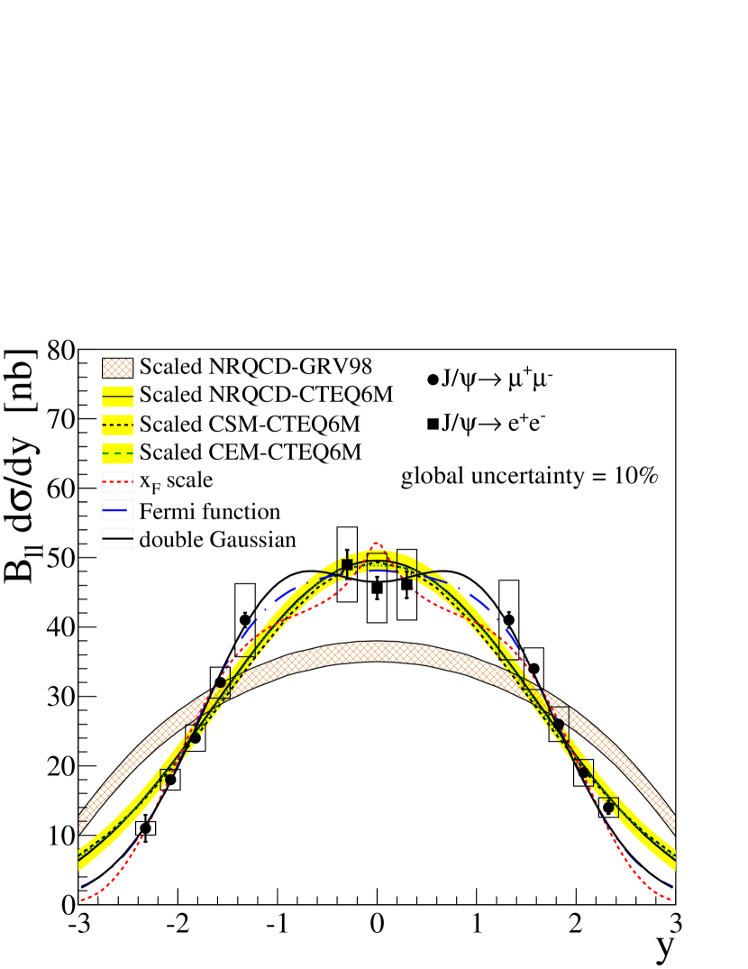
Figure 18: (Color online)Rapidity dependence of the $J/\psi~{}$yield combining dielectron ($|y|<0.35$ - full squares) with dimuon channels ($1.2<|y|<2.4$ - full circles) along with the fits used to estimate the total cross section. Lines correspond to the three fitting functions described in the text. Also shown are arbitrarily normalized model predictions (NRQCD Cooper et al. (2004), CEM Frawley et al. (2008); Vogt (2009) and CSM Lansberg (2010)).

The rapidity distribution of the $J/\psi~{}$dilepton cross section is shown in Fig. 18 and in Table 9. The data points are grouped into three rapidity ranges, corresponding to the different detectors used in the measurement: south muon arm ($-2.4<y<-1.2$), central arms ($|y|<0.35$) and north muon arm ($1.2<y<2.4$). The systematic uncertainties represented by the boxes are point-to-point correlated for data points in the same group and are uncorrelated between different groups. All points have a global uncertainty of 10% coming from the minimum-bias trigger efficiency estimate.

In order to compare the shape of the rapidity distribution, we normalized the CEM, CSM and NRQCD predictions to the integral of the measured data in Fig.18. All models use the CTEQ6M PDFs. The NRQCD model is also available with the GRV98 and the MRST99 PDFs. The theoretical rapidity distributions exhibit a similar shape when using CTEQ6M. A very different rapidity distribution is obtained when the NRQCD prediction is calculated using GRV98 and MRST99 (MRST99 is not shown in the figure). These observations suggest that the choice of PDF plays the most important role in describing the shape of the $J/\psi~{}$rapidity distribution. The rapidity shape also appears to be independent of the feed-down contributions, since the CSM has a similar shape to the CEM and NRQCD model, despite the fact that it contains only direct $J/\psi~{}$contributions. The PDF which best describes the data is CTEQ6M and we use this for the remaining comparisons.

An empirical description of the $J/\psi~{}$yield used in some fixed-target experiments with large coverage is based on the Feynman $x_{F}$ form Schub et al. (1995),

$$\frac{d\sigma}{dx_{F}} = A\left(1-|x_{F}|\right)^{c}.$$ (17)

We can convert to a rapidity distribution by writing

$$\frac{d\sigma}{dy} = \frac{d\sigma}{dx_{F}}\frac{dx_{F}}{dy}$$

$$\approx 2A\left(1-|x_{F}|\right)^{c}\sqrt{\frac{\left<p_{T}^{2}\right>+M_{J/\psi}^{2}}{s}}\cosh{y}$$

where $p_{T}=1.73$ GeV/$c~{}$is the average of the $J/\psi~{}$$p_{T}$ distributions over all measured rapidities. The fit returned $c=16.3\pm 0.4$ with $\chi^{2}$ probability of 31%, where statistical and systematic uncertainties are summed in quadrature(Fig. 18). Fig. 19 shows that $c$ scales approximately as $c=a/\left(1+b/\sqrt{s}\right)$. This extrapolation of the rapidity dependence can be used to estimate the total cross section from measurements with limited rapidity coverage and will be used as one method to calculate the total cross section from the present measurement.

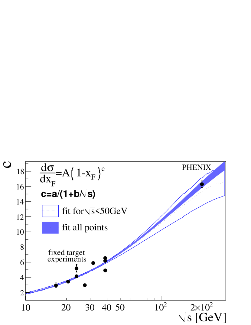
Figure 19: (Color online) Energy dependence of the parameter $c$ where $d\sigma/dx_{F}=(1-x_{F})^{c}$ is fitted to $x_{F}$ distributions of $J/\psi~{}$production in fixed target experiments Anderson et al. (1976); Branson et al. (1977); Binkley et al. (1976); Antoniazzi et al. (1992); Siskind et al. (1980); Gribushin et al. (2000); Schub et al. (1995); Alexopoulos et al. (1997) and in the PHENIX rapidity distribution. The parameters ($a=27.8\pm 1.5$, $b=(143\pm 11)$ GeV) are obtained from a fit to the experimental data points.

VI.2 Total cross section of inclusive $J/\psi~{}$

The total cross section was estimated from different empirical functions fitted to the rapidity distribution - a double Gaussian,the $x_{F}$ scaling function (VI.1) described above, and a “Fermi” function:

$$\frac{d\sigma}{dy}=\frac{A}{1+e^{\frac{(y-\lambda)}{\sigma}}}$$ (19)

Rapidity distributions based on charmonium production models were not used in the total cross section in order to avoid any theoretical bias.

The correlated uncertainties between data points measured in each spectrometer were propagated to the fit uncertainty by allowing the points to move coherently in the rapidity range covered by that spectrometer. Table 4 shows the total dilepton cross section and the $\chi^{2}$ probability for each function used in the fit. The final cross section is obtained from the average of the numbers from each fit function weighted according to their $\chi^{2}$ probability. The systematic uncertainty from the unknown rapidity shape is taken from the standard deviation between the three fitting functions. Based on these fits, we conclude that the PHENIX rapidity acceptance covers 56 $\pm$ 2 % of the total $J/\psi~{}$cross section. The $J/\psi~{}$cross section reported in this paper is $180.7\pm 2.0^{\rm stat}\pm 11^{\rm syst}nb$, in agreement with our previous result with a reduction in the statistical and systematic uncertainties.

Table 4: Estimate of the total dilepton $J/\psi~{}$cross section from the three fitting functions, together with the weighted average and a comparison to the result obtained in our previous measurement. The measured total cross sections have an additional 10% global uncertainty.

estimating function	$\chi^{2}$ prob.	$B_{ll}\sigma_{\mbox{$J/\psi~{}$}}(nb)$
$x_{F}$ scale fcn, Eq.VI.1	0.30	$170.8\pm 1.5^{\rm stat}\pm 9^{\rm syst}$
double Gaussian	0.79	$183.5\pm 1.9^{\rm stat}\pm 11^{\rm syst}$
Fermi fcn, Eq.19	0.70	$182.0\pm 2.3^{\rm stat}\pm 12^{\rm syst}$
AVERAGE		$180.7\pm 2.0^{\rm stat}\pm 12^{\rm syst}$
2005 Run resultAdare et al. (2007a)		$178\pm 3.0^{\rm stat}\pm 53^{\rm syst}$

Table 5 presents the measured total $J/\psi~{}$cross section and the expectations from the three production models considered in this text. The experimental direct $J/\psi~{}$cross section is estimated assuming that the feed-down fraction of $\chi_{c}$ and $\psi^{\prime}~{}$measured at midrapidity is the same at forward rapidity. The feed-down from $B$ mesons is only significant at high $p_{T}$ and is not considered in the total cross section. The total cross section estimated using the CEM is the only one which agrees with the experimental result, although the cross section calculation includes the scale factor $\mathcal{F}$ (Sec. I) obtained from $J/\psi~{}$measurements. The NRQCD includes color singlet and color octet states, and as mentioned at the beginning of this section, cannot be extrapolated to low $p_{T}$ to obtain the rapidity distribution without the addition of an empirical constraint.

Table 5: Comparison of the measured $J/\psi~{}$cross section with the three models considered in this text. Direct $J/\psi~{}$cross sections are obtained assuming that the $\chi_{c}$ and $\psi^{\prime}~{}$feed-down fractions measured at midrapidity are the same at forward rapidity. Type A, type B and type C errors are quadratically summed in the measured result.

	direct $J/\psi~{}$	inclusive
CEM	-	169 $\pm$ 30 nb
NLO CSM	53 $\pm$ 26 nb	-
LO NRQCD	-	140 $\pm$ 5 nb
Measured	105 $\pm$ 26 nb	181 $\pm$ 22 nb

VI.3 $J/\psi~{}$$p_{T}$ distribution

The $p_{T}$ -dependent dielectron differential cross section at midrapidity is compared to other $p$+$p$ and $p+\bar{p}$ experiments in Fig. 20(a). The shapes of the transverse momentum distributions follow the well known ”thermal” exponential behavior for $p_{T}<2$ GeV/$c~{}$and a hard-scattering power law behavior at high $p_{T}$ . The hard process scales with $x_{T}=2p_{T}/\sqrt{s}$ ($\sqrt{s}^{n}Ed^{3}\sigma/d^{3}p=G(x_{T})$) Adcox et al. (2005) for all collision energies, as can be seen in Fig. 20(b), where $n=5.6\pm 0.2$ Abelev et al. (2009). n is related to the number of partons involved in the interaction. A pure LO process leads to $n=4$, hence, NLO terms may be important in $J/\psi~{}$production.Berman et al. (1971); Blankenbecler et al. (1975, 1972); Cahalan et al. (1975)

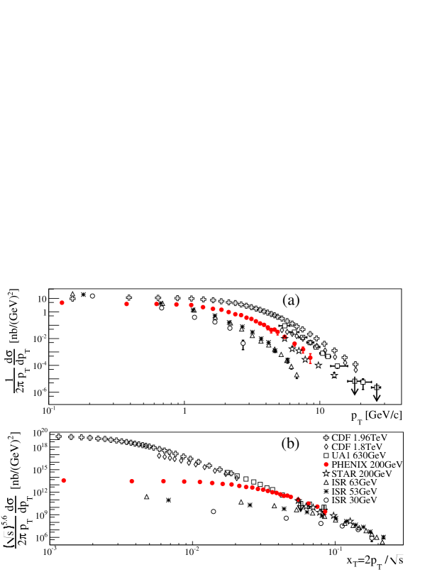
Figure 20: (Color online) $p_{T}$ distribution (a) and $x_{T}$ distribution (b) of $J/\psi~{}$yield in PHENIX, STAR Abelev et al. (2009), ISR Clark et al. (1978), UA1 Albajar et al. (1991) and CDFAbe et al. (1997a); Acosta et al. (2005) at $y\sim 0$.

The $p_{T}$ dependence of the $J/\psi~{}$differential cross sections measured at forward and midrapidity are shown in Fig. 21 along with theoretical calculations where the absolute normalization is determined in the calculations. The CEM and the NRQCD (for $p_{T}>2$ GeV/$c~{}$) provide reasonable descriptions of the $p_{T}$ distribution, whereas the CSM disagrees in both the normalization and the slope of the $p_{T}$ distribution, indicating that NLO color singlet intermediate states cannot account for the direct $J/\psi~{}$production. However, the NLO CSM calculation gives a good description of the $J/\psi~{}$polarization measured by PHENIX Adare et al. (2010a); Lansberg (2010). Attempts are being made to extend the CSM to NNLO. Preliminary NNLO CSM calculations performed for $p_{T}>5$ GeV/$c~{}$Lansberg (2010) shows a large increase in the yield, but still under- predict the experimental results. None of these theoretical models consider the $B$-meson decay contribution to the $J/\psi~{}$yield. The fixed-order plus next-to-leading-log (FONLL) Cacciari et al. (2005) calculation of these decays is also plotted in Fig. 21 and has a reasonable agreement with STAR measurements using $J/\psi~{}$-hadron correlations Abelev et al. (2009). According to this calculation, the $B$-meson contribution to the measured $J/\psi~{}$inclusive yield is between 2%(1%) at 1 GeV/$c~{}$and 20%(15%) at 7.5 GeV/$c~{}$in the mid(forward)-rapidity region with large theoretical uncertainties.

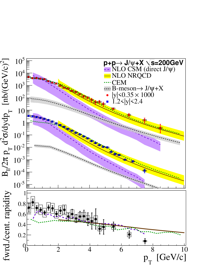
Figure 21: (Color online) Top: Transverse momentum dependence of $J/\psi~{}$yield in $|y|<0.35$ and $1.2<|y|<2.4$ along with predictions based on CSM Lansberg (2010), NRQCD Butenschön and Kniehl (2011), CEM Vogt (2009); Frawley et al. (2008) and $B$-meson decay based on FONLL calculation Cacciari et al. (2005). All models use CTEQ6M. Theoretical uncertainties are represented as bands. Note that the midrapidity points are scaled up by a factor of 1000. Bottom: Ratio of the forward and central rapidity $p_{T}$ spectra and corresponding theoretical predictions.

The $p_{T}$ dependence of the $J/\psi~{}$yield is harder at midrapidity, as seen from the ratio between the forward and midrapidity differential cross sections versus $p_{T}$ shown in Fig. 21(bottom). The figure also includes the forward/midrapidity yield ratios from the theoretical models using their mean values and assuming that theoretical uncertainties in these ratios cancel out. All of the models predict a downward trend, but the CEM and NRQCD calculations do not follow a slope as large as the data.

The mean transverse momentum squared $\left<p_{T}^{2}\right>$ was calculated numerically from the $p_{T}$ distribution. The correlated uncertainty was propagated to $\left<p_{T}^{2}\right>$ by moving low-$p_{T}$ and high-$p_{T}$ data points coherently in opposite directions according to their type B uncertainty. The results with the propagated type A and type B uncertainties are listed in Table 6. The table also contains $\left<p_{T}^{2}\right>$ for $p_{T}<$ 5 GeV/$c~{}$for a direct comparison with previous PHENIX results Adare et al. (2008). As expected, the mean transverse momentum squared at midrapidity is larger than at forward rapidity.

Table 6: Mean transverse momentum squared in $(\mbox{GeV/$c~{}$})^{2}$ of $J/\psi~{}$and $\psi^{\prime}~{}$for different rapidity and $p_{T}$ ranges. Uncertainties are type A and type B respectively.

system	$\left<p_{T}^{2}\right>$	$\left.\left<p_{T}^{2}\right>\right|_{p_{T}<5GeV/c}$
$J/\psi~{}$$1.2<|y|<2.4$	3.65$\pm$0.03$\pm$0.09	3.45$\pm$0.03$\pm$0.08
$J/\psi~{}$$|y|<0.35$	4.41$\pm$0.14$\pm$0.11	3.89$\pm$0.11$\pm$0.09
$\psi^{\prime}~{}$$|y|<0.35$	4.7 ${}^{+1.5}_{-1.05}$ $\pm$0.2	4.7${}^{+1.5}_{-1.05}$ $\pm$0.2

VI.4 Charmonia ratios and $J/\psi~{}$feed-down fractions

The transverse momentum dependence of the $\mbox{$\psi^{\prime}~{}$}/(\mbox{$J/\psi~{}$})$ yield ratio (Fig. 6, bottom) is consistent with that observed in other experiments. Fig. 22 shows the collision energy dependence of the $\mbox{$\psi^{\prime}~{}$}/(\mbox{$J/\psi~{}$})$ yield ratio in light fixed target experiments and $p$+$p$ or $p+\bar{p}$ colliders. In this figure, the ratios from $p+\bar{p}$ experiments were calculated using the reported $J/\psi~{}$and $\psi^{\prime}~{}$cross sections for $p_{T}>5$ GeV/$c~{}$together with their point-to-point uncorrelated uncertainties. The $B$ meson decay contribution was removed from the $J/\psi~{}$and $\psi^{\prime}~{}$yields, in the case of the CDF experiment. Only E705 has broad coverage ($-0.1<x_{F}<0.5$). The other experiments in this figure have a rapidity coverage of $|y|<0.6$. A weak trend of increasing $\mbox{$\psi^{\prime}~{}$}/(\mbox{$J/\psi~{}$})$ yield ratio for higher collision energy (Fig. 22) and for higher $p_{T}$ (Fig. 6) can be observed. As mentioned earlier, the $\psi^{\prime}~{}$feed-down fraction of (9.7 $\pm$ 2.4)% is in agreement with the world average of $(8.1\pm 0.3)$% calculated in Faccioli et al. (2008).

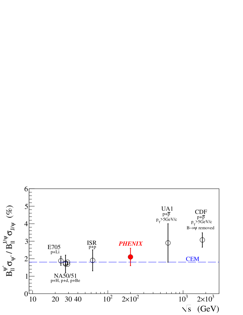
Figure 22: (Color online) Collision energy dependence of the $\mbox{$\psi^{\prime}~{}$}/(J/\psi)$ dilepton cross section ratio obtained in $p$+$p$ and light fixed target $p$+A collisions Antoniazzi et al. (1993); Abreu et al. (1998); Alessandro et al. (2006); Clark et al. (1978); Albajar et al. (1991); Abe et al. (1997a) compared to the CEM estimate Frawley et al. (2008). Statistical and systematic errors were quadratically summed.

The feed-down fraction obtained from our $\mbox{$\chi_{c}$~{}}\rightarrow\mbox{$J/\psi~{}$}+\gamma$ measurement is compared with other experiments over a broad range of collision energy and $x_{F}$, as well as over many different colliding species (Fig. 23). The value measured in this work, $F_{\chi_{c}}^{J/\psi}=(32\pm 9)\%$, is consistent with the world average of ($25\pm 5$)% after accounting for $A$ dependencies in the fixed target experiments Faccioli et al. (2008).

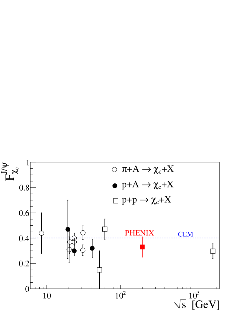
Figure 23: (Color online)Collision energy dependence of $\chi_{c}$ feed-down to $J/\psi~{}$measured in $p$+$p$ and $p$+A collisions Hahn et al. (1984); Antoniazzi et al. (1993); Alexopoulos et al. (2000); Abt et al. (2003); Binon et al. (1984); Lemoigne et al. (1982); Koreshev et al. (1996); Kourkoumelis et al. (1979); Abe et al. (1997b) compared to the CEM calculation Frawley et al. (2008).

Combining the results of feed down from the $\psi^{\prime}~{}$and the $\chi_{c}$ we obtain a total $J/\psi~{}$feed-down fraction measured in the midrapidity region of $(42\pm 9)$%.

VI.5 Outcomes for heavy ion collisions.

The feed-down fractions from the $\psi^{\prime}~{}$and $\chi_{c}$have important implications for survival rates of charmonium states when either ordinary nuclear matter or high energy density nuclear matter is involved. Because of their larger size compared to the $J/\psi~{}$, excited charmonium states may have a different breakup cross section in nuclear matter. This effect can modify the feed-down fractions in $p$+A collisions. On the other hand, if the $c\bar{c}~{}$is not formed as a color singlet, it can cross the nuclear matter as a colored preresonant state Vogt (2002). If this were true, the breakup cross section of $J/\psi~{}$and $\psi^{\prime}~{}$should be the same and there would be no modification of the $\psi^{\prime}~{}$feed-down fraction in $p$+A collisions, whereas a possible modification can occur for the $\chi_{c}$ since it is expected to be formed mainly as a color singlet. Given the large statistical uncertainties in all measured $\psi^{\prime}~{}$/ ($J/\psi~{}$) ratios shown in Figs. 6 and 22, differences between $p+p$ and $p$+A are impossible to see, and therefore no conclusion about possible cold nuclear matter effects can be made at this time. The same is true for the $\chi_{c}$ feed-down fraction in Fig. 23. Higher precision measurements of charmonium states in $p$+$p$ and $d$+Au collisions in the future may allow an improved determination of these possible cold nuclear matter effects on the feed-down fraction.

The behavior of charmonium states in the high density, hot nuclear matter created in heavy ion collisions, has long been of interestMatsui and Satz (1986). Spectral function computations Mócsy and Petreczky (2007) indicate that the $\chi_{c}$ and $\psi^{\prime}~{}$states should dissociate at a lower temperature in hot nuclear matter, due to color screening, than the $J/\psi$. One of the most important implications of the observed feed-down fractions is that the complete dissociation of the $\chi_{c}$ and $\psi^{\prime}~{}$states would lead to a (42 $\pm$ 9)% $J/\psi~{}$suppression. The measured nuclear modification factor of $J/\psi~{}$mesons in central Au+Au collisions at $\sqrt{s}=$ 200 GeV Adare et al. (2007b) implies a suppression of (74 $\pm$ 6)% at midrapidity and (84 $\pm$ 6)% at forward rapidity. Hence, the complete dissociation of the excited states of charmonium and the associated loss of the $J/\psi~{}$yield cannot completely explain its suppression observed in Au+Au collisions. Cold nuclear matter effects and the possible dissociation of direct $J/\psi~{}$by color-screening could presumably account for the remaining suppression.

VII Summary and Conclusions

In conclusion, we have measured the yields of the three most important charmonium states in $p$+$p$ collisions at $\sqrt{s}=$ 200 GeV, where gluon fusion is expected to be the dominant production process. The rapidity dependence of $J/\psi~{}$supports the use of CTEQ6M to describe the gluon distribution in protons. The inclusive $J/\psi~{}$yield is in agreement with current models which involve a initial formation of colored charmonium states, as in the CEM or the color octet states of the NRQCD models. The inclusive $J/\psi~{}$yield observed at midrapidity is composed of $9.6\pm 2.4$% of $\psi^{\prime}~{}$decays and $32\pm 9$% of $\chi_{c}$ decays. This result is in agreement with what was observed in other experiments. Given the current large statistical uncertainties, no conclusion can be made about collision energy or $p_{T}$ dependence of these fractions. Finally, this $J/\psi~{}$cross section measurement and feed-down fractions will play an important role in current studies of cold nuclear matter and the hot, dense matter formed in heavy ion collisions.

Appendix A Data Tables

Table 7: $J/\psi~{}$differential cross section in the midrapidity region ($|y|<0.35$) followed by point-to-point uncorrelated (statistical and uncorrelated systematic uncertainties) and correlated systematic uncertainties. Global uncertainty is 10%.

$p_{T}$ [GeV/$c~{}$]	$\frac{1}{2\pi p_{T}}\frac{B_{ee}d^{2}\sigma_{J/\psi}}{dydp_{T}}[nb/(\mbox{GeV/$c~{}$})^{2}]$
	value	uncor.	corr.
0-0.25	4.9	0.5	0.6
0.25-0.5	3.9	0.3	0.5
0.5-0.75	3.9	0.2	0.5
0.75-1	3.5	0.2	0.4
1-1.25	3.19	0.17	0.38
1.25-1.5	2.21	0.14	0.27
1.5-1.75	1.69	0.12	0.2
1.75-2	1.42	0.1	0.17
2-2.25	95	8	12	$\times 10^{-2}$
2.25-2.5	66	7	8	$\times 10^{-2}$
2.5-2.75	56	6	7	$\times 10^{-2}$
2.75-3	37	5	5	$\times 10^{-2}$
3-3.25	29	4	4	$\times 10^{-2}$
3.25-3.5	19.9	${}^{+3.5}_{-3.6}$	2.4	$\times 10^{-2}$
3.5-3.75	13.6	2.8	1.7	$\times 10^{-2}$
3.75-4	10.6	2.5	1.3	$\times 10^{-2}$
4-4.25	6.89	${}^{+2.3}_{-2.2}$	0.8	$\times 10^{-2}$
4.25-4.5	4.4	${}^{+1.7}_{-1.6}$	0.5	$\times 10^{-2}$
4.5-4.75	4.7	${}^{+1.5}_{-1.4}$	0.6	$\times 10^{-2}$
4.75-5	3.1	1.2	0.4	$\times 10^{-2}$
5-6	1.35	${}^{+0.31}_{-0.32}$	${}^{+0.17}_{-0.18}$	$\times 10^{-2}$
6-7	4.1	1.3	${}^{+0.5}_{-0.6}$	$\times 10^{-3}$
7-8	1.6	0.7	0.2	$\times 10^{-3}$
8-9	0.37	${}^{+0.37}_{-0.22}$	${}^{+0.05}_{-0.06}$	$\times 10^{-3}$

Table 8: $\psi^{\prime}~{}$differential cross section at $|\eta|<$0.35 followed by point-to-point uncorrelated (statistical and uncorrelated systematic uncertainties) and correlated systematic uncertainties. Global uncertainty is 10%.

$p_{T}$ [GeV/$c~{}$]	$\frac{1}{2\pi p_{T}}\frac{B_{ee}d^{2}\sigma_{\psi^{\prime}}}{dydp_{T}}$ [pb/$(\mbox{GeV/$c~{}$})^{2}$]
	value	uncor.	corr.
0-1	67	20	9
1-2	40	11	${}^{+7}_{-6}$
2-3	15	6	3
3-5	2.7	${}^{+2.5}_{-1.5}$	0.5
5-7	$<$2.25 (90% CL)
0-5	95	20	${}^{+17}_{-15}$

Table 9: Rapidity dependence of $J/\psi~{}$yield followed by point-to-point uncorrelated (statistical and uncorrelated systematic uncertainties) and correlated systematic uncertainties. Global uncertainty is 10%.

rapidity	$B_{ll}\frac{d\sigma_{J/\psi}}{dy}[nb]$
	value	uncor.	corr.
-2.325	10.9	1.9	1.0
-2.075	17.6	0.5	1.5
-1.825	24.4	0.4	1.9
-1.575	31.5	0.5	2.2
-1.325	41.2	1.1	5.3
-0.3	49.0	2.1	5.4
0.0	45.6	1.6	5.0
0.3	46.1	1.9	5.1
1.325	40.7	1.2	5.7
1.575	33.6	0.7	3.0
1.825	25.6	0.4	2.5
2.075	18.9	0.4	1.9
2.325	13.9	0.9	1.4

Table 10: $\psi^{\prime}~{}$/ ($J/\psi~{}$) dielectron yield ratio measured at $|\eta|<$0.35 followed by point-to-point uncorrelated (statistical and uncorrelated systematic uncertainties) and correlated systematic uncertainties.

$p_{T}$ [GeV/$c~{}$]	$\frac{B_{ee}^{\psi^{\prime}}\sigma_{\psi^{\prime}}}{B_{ee}^{J/\psi}\sigma_{J/\psi}}$ [%]
	value	uncor.	corr.
0-1	1.69	0.51	${}^{+0.12}_{-0.11}$
1-2	1.96	0.53	${}^{+0.23}_{-0.15}$
2-3	2.3	1.0	${}^{+0.5}_{-0.3}$
3-5	3.4	${}^{+2.0}_{-2.1}$	${}^{+0.5}_{-0.4}$
5-7	$<$38 (90% CL)
0-5	2.1	0.5

Table 11: Di-muon $J/\psi~{}$yield in the forward rapidity region (1.2$<|y|<$2.4) followed by point-to-point uncorrelated (statistical and uncorrelated systematic uncertainties) and correlated systematic uncertainties. Global uncertainty is 10%.

$p_{T}$ [GeV/$c~{}$]	$\frac{1}{2\pi p_{T}}\frac{B_{\mu\mu}d^{2}\sigma_{J/\psi}}{dydp_{T}}[nb/(\mbox{GeV/$c~{}$})^{2}]$
	value	uncor.	corr.
0.125	3.49	0.14	0.50
0.375	3.28	0.08	0.49
0.625	2.85	0.06	0.40
0.875	2.43	0.05	0.16
1.125	2.04	0.04	0.18
1.375	1.57	0.03	0.16
1.625	1.194	0.024	0.12
1.875	85.1	1.9	7.9	$\times 10^{-2}$
2.125	63.8	1.6	5.6	$\times 10^{-2}$
2.375	46.8	1.2	3.7	$\times 10^{-2}$
2.625	31.5	0.9	2.5	$\times 10^{-2}$
2.875	22.1	0.7	1.7	$\times 10^{-2}$
3.125	15.3	0.6	1.1	$\times 10^{-2}$
3.375	11.1	0.5	0.8	$\times 10^{-2}$
3.625	7.7	0.4	0.6	$\times 10^{-2}$
3.875	5.53	0.27	0.37	$\times 10^{-2}$
4.125	3.28	0.21	0.23	$\times 10^{-2}$
4.375	2.26	0.16	0.15	$\times 10^{-2}$
4.625	1.45	0.13	0.10	$\times 10^{-2}$
4.875	1.06	0.11	0.08	$\times 10^{-2}$
5.125	1.02	0.10	0.07	$\times 10^{-2}$
5.375	4.3	0.6	0.4	$\times 10^{-3}$
5.625	2.9	0.4	0.2	$\times 10^{-3}$
5.875	2.4	0.4	0.2	$\times 10^{-3}$
6.25	1.02	0.15	0.09	$\times 10^{-3}$
6.75	0.73	0.13	0.06	$\times 10^{-3}$
7.5	0.13	0.04	0.012	$\times 10^{-3}$

References

- Matsui and Satz (1986) T. Matsui and H. Satz, Phys. Lett. B178, 416 (1986).
- Mócsy and Petreczky (2007) A. Mócsy and P. Petreczky, Phys. Rev. Lett. 99, 211602 (2007).
- Cacciari et al. (2005) M. Cacciari, P. Nason, and R. Vogt, Phys. Rev. Lett. 95, 122001 (2005).
- Adare et al. (2006a) A. Adare et al. (PHENIX Collaboration), Phys. Rev. Lett. 97, 252002 (2006a).
- Fritzsch (1977) H. Fritzsch, Phys. Lett. B67, 217 (1977).
- Amundson et al. (1997) J. F. Amundson, O. J. P. Eboli, E. M. Gregores, and F. Halzen, Phys. Lett. B390, 323 (1997).
- Baier and Ruckl (1981) R. Baier and R. Ruckl, Phys. Lett. B102, 364 (1981).
- Cho and Leibovich (1996) P. L. Cho and A. K. Leibovich, Phys. Rev. D 53, 6203 (1996).
- Abe et al. (1997a) F. Abe et al. (CDF Collaboration), Phys. Rev. Lett. 79, 572 (1997a).
- Adare et al. (2007a) A. Adare et al. (PHENIX Collaboration), Phys. Rev. Lett. 98, 232002 (2007a).
- Campbell et al. (2007) J. M. Campbell, F. Maltoni, and F. Tramontano, Phys. Rev. Lett. 98, 252002 (2007).
- Artoisenet et al. (2007) P. Artoisenet, J. P. Lansberg, and F. Maltoni, Phys. Lett. B653, 60 (2007).
- Gong and Wang (2008) B. Gong and J.-X. Wang, Phys. Rev. Lett. 100, 232001 (2008).
- Artoisenet et al. (2008) P. Artoisenet, J. M. Campbell, J. P. Lansberg, F. Maltoni, and F. Tramontano, Phys. Rev. Lett. 101, 152001 (2008).
- Lansberg (2009a) J. P. Lansberg, Eur. Phys. J. C61, 693 (2009a).
- Lansberg (2009b) J. P. Lansberg, Phys. Lett. B679, 340 (2009b).
- Lansberg (2010) J. P. Lansberg (2010), eprint 1003.4319.
- Adare et al. (2010a) A. Adare et al., Phys. Rev. D 82, 012001 (2010a).
- Abulencia et al. (2007) A. Abulencia et al. (CDF Collaboration), Phys. Rev. Lett. 99, 132001 (2007).
- Butenschön and Kniehl (2011) M. Butenschön and B. A. Kniehl, Phys. Rev. Lett. 106, 022003 (2011).
- Acosta et al. (2005) D. Acosta et al. (CDF Collaboration), Phys. Rev. D 71, 032001 (2005).
- Adloff et al. (2002) C. Adloff et al. (H1 Collaboration), Eur. Phys. J. C25, 25 (2002).
- Aaron et al. (2010) F. D. Aaron et al. (H1 Collaboration), Eur. Phys. J. C68, 401 (2010).
- Gong et al. (2009) B. Gong, X. Q. Li, and J.-X. Wang, Physics Letters B 673, 197 (2009), ISSN 0370-2693.
- Adare et al. (2010b) A. Adare et al. (2010b).
- Adare et al. (2011) A. Adare et al. (2011), eprint 1103.6269.
- Adare et al. (2007b) A. Adare et al. (PHENIX Collaboration), Phys. Rev. Lett. 98, 232301 (2007b).
- Adcox et al. (2003) K. Adcox et al. (PHENIX Collaboration), Nucl. Instrum. Meth. A499, 469 (2003).
- Akikawa et al. (2003) H. Akikawa et al. (PHENIX Collaboration), Nucl. Instrum. Meth. A499, 537 (2003).
- Adler et al. (2003) S. S. Adler et al., Phys. Rev. Lett. 91, 241803 (2003).
- Adare et al. (2010c) A. Adare et al. (PHENIX Collaboration) (2010c).
- Adare et al. (2010d) A. Adare et al., Phys. Rev. C 81, 034911 (2010d).
- Vogelsang (2007) W. Vogelsang (2007), private communication.
- Spiridonov (2004) A. Spiridonov (2004), eprint hep-ex/0510076.
- Adare et al. (2006b) A. Adare et al. (PHENIX Collaboration), Phys. Rev. Lett. 97, 252002 (2006b).
- Adare et al. (2009a) A. Adare et al., Phys. Rev. Lett. 103, 082002 (2009a).
- Aggarwal et al. (2010) M. M. Aggarwal et al. (STAR Collaboration), Phys. Rev. Lett. 105, 202301 (2010).
- Sjostrand et al. (2006) T. Sjostrand, S. Mrenna, and P. Skands, JHEP 05, 026 (2006).
- Norrbin and Sjostrand (2000) E. Norrbin and T. Sjostrand, Eur. Phys. J. C17, 137 (2000).
- Pumplin et al. (2002) J. Pumplin et al., JHEP 07, 012 (2002).
- (41) GEANT 3.2.1, CERN Computing Library (????), http://wwwasdoc.web.cern.ch/wwwasdoc/pdfdir/geant.pdf.
- Adare et al. (2009b) A. Adare et al. (PHENIX Collaboration), Phys. Lett. B670, 313 (2009b).
- Adare et al. (2009c) A. Adare et al. (PHENIX Collaboration), Phys. Rev. Lett. 103, 082002 (2009c).
- Armstrong et al. (1996) T. A. Armstrong et al., Phys. Rev. D 54, 7067 (1996).
- Amsler et al. (2008 and 2009 partial update for the 2010 edition) C. Amsler et al. (Particle Data Group), Phys. Lett. B667, 1 (2008 and 2009 partial update for the 2010 edition).
- Aphecetche et al. (2003) L. Aphecetche et al. (PHENIX Collaboration), Nucl. Instrum. Meth. A499, 521 (2003).
- Sridhar (1993) K. Sridhar, Phys.Rev.Lett. 70, 1747 (1993).
- PPG121 (2010) PPG121 (2010), under preparation.
- Frawley et al. (2008) A. D. Frawley, T. Ullrich, and R. Vogt, Phys. Rept. 462, 125 (2008).
- Vogt (2009) R. Vogt (2009), private communication.
- Cooper et al. (2004) F. Cooper, M. X. Liu, and G. C. Nayak, Phys. Rev. Lett. 93, 171801 (2004).
- Schub et al. (1995) M. H. Schub et al. (E789 Collaboration), Phys. Rev. D 52, 1307 (1995).
- Anderson et al. (1976) K. J. Anderson et al., Phys. Rev. Lett. 37, 799 (1976).
- Branson et al. (1977) J. G. Branson et al., Phys. Rev. Lett. 38, 1331 (1977).
- Binkley et al. (1976) M. E. Binkley et al., Phys. Rev. Lett. 37, 574 (1976).
- Antoniazzi et al. (1992) L. Antoniazzi et al. (E705 Collaboration), Phys. Rev. D 46, 4828 (1992).
- Siskind et al. (1980) E. J. Siskind et al., Phys. Rev. D 21, 628 (1980).
- Gribushin et al. (2000) A. Gribushin et al. (E672 Collaboration), Phys. Rev. D 62, 012001 (2000).
- Alexopoulos et al. (1997) T. Alexopoulos et al. (E771 Collaboration), Phys. Rev. D 55, 3927 (1997).
- Adcox et al. (2005) K. Adcox et al. (PHENIX Collaboration), Nucl. Phys. A757, 184 (2005).
- Abelev et al. (2009) B. I. Abelev et al. (STAR Collaboration), Phys. Rev. C 80, 041902 (2009).
- Berman et al. (1971) S. Berman, J. Bjorken, and J. B. Kogut, Phys. Rev. D 4, 3388 (1971).
- Blankenbecler et al. (1975) R. Blankenbecler, S. J. Brodsky, and J. Gunion, Phys. Rev. D 12, 3469 (1975).
- Blankenbecler et al. (1972) R. Blankenbecler, S. J. Brodsky, and J. Gunion, Phys.Lett. B42, 461 (1972).
- Cahalan et al. (1975) R. Cahalan, K. Geer, J. B. Kogut, and L. Susskind, Phys. Rev. D 11, 1199 (1975).
- Clark et al. (1978) A. G. Clark et al., Nucl. Phys. B142, 29 (1978).
- Albajar et al. (1991) C. Albajar et al. (UA1 Collaboration), Phys. Lett. B256, 112 (1991).
- Adare et al. (2008) A. Adare et al. (PHENIX Collaboration), Phys. Rev. Lett. 101, 122301 (2008).
- Faccioli et al. (2008) P. Faccioli, C. Lourenco, J. Seixas, and H. K. Woehri, JHEP 10, 004 (2008).
- Antoniazzi et al. (1993) L. Antoniazzi et al. (E705 Collaboration), Phys. Rev. Lett. 70, 383 (1993).
- Abreu et al. (1998) M. C. Abreu et al. (NA51 Collaboration), Phys. Lett. B438, 35 (1998).
- Alessandro et al. (2006) B. Alessandro et al. (NA50 Collaboration), Eur. Phys. J. C48, 329 (2006).
- Hahn et al. (1984) S. R. Hahn et al., Phys. Rev. D 30, 671 (1984).
- Alexopoulos et al. (2000) T. Alexopoulos et al. (E771 Collaboration), Phys. Rev. D 62, 032006 (2000).
- Abt et al. (2003) I. Abt et al. (HERA-B Collaboration), Phys. Lett. B561, 61 (2003).
- Binon et al. (1984) F. G. Binon et al. (Serpukhov-Brussels-Annecy (LAPP) Collaboration), Nucl. Phys. B239, 311 (1984).
- Lemoigne et al. (1982) Y. Lemoigne et al., Phys. Lett. B113, 509 (1982).
- Koreshev et al. (1996) V. Koreshev et al. (E672 and E706 Collaborations), Phys. Rev. Lett. 77, 4294 (1996).
- Kourkoumelis et al. (1979) C. Kourkoumelis et al., Phys. Lett. B81, 405 (1979).
- Abe et al. (1997b) F. Abe et al. (CDF Collaboration), Phys. Rev. Lett. 79, 578 (1997b).
- Vogt (2002) R. Vogt, Nuclear Physics A 700, 539 (2002), ISSN 0375-9474, URL http://www.sciencedirect.com/science/article/B6TVB-44B25SB-2/2/351cdf30b1138b0118c9c98a5f91ead0.