Longitudinal excitations in quantum antiferromagnets

Abstract

By extending our recently proposed magnon-density-waves to low dimensions, we investigate, using a microscopic many-body approach, the longitudinal excitations of the quasi-one-dimensional (quasi-1d) and quasi-2d Heisenberg antiferromagnetic systems on a bipartite lattice with a general spin quantum number. We obtain the full energy spectrum of the longitudinal mode as a function of the coupling constants in the original lattice Hamiltonian and find that it always has a non-zero energy gap if the ground state has a long-range order and becomes gapless for the pure isotropic 1d model. The numerical value of the minimum gap in our approximation agrees with that of a longitudinal mode observed in the quasi-1d antiferromagnetic compound KCuF₃ at low temperature. It will be interesting to compare values of the energy spectrum at other momenta if their experimental results are available.

I introduction

The low temperature properties of many two-dimensional (2d) and three-dimensional (3d) quantum antiferromagnetic systems can be understood by Anderson’s spin wave theory (SWT) and its extensions ande , which provides correct description of the quantum corrections to the classical Néel states of the systems. For many purposes, the dynamics of these systems at low temperature can be considered as that of a dilute gas of weakly interacting spin-wave quasiparticles (magnons) with its density corresponding to the quantum correction to the classical Néel order; also present in these systems are the longitudinal fluctuations consisting of the multi-magnon continuum hube .

On the other hand, due to the strong quantum fluctuations, the isotropic 1d antiferromagnets with low quantum spin numbers exhibit different low temperature properties, such as no Néel-like long-range order in the ground state and the quite different low-lying excitation states from the 2d and 3d counterparts. According to the exact solutions by Bethe ansatz, the natural low-lying excitation states of the 1d spin-1/2 Heisenberg model have been shown corresponding to the spin-1/2 objects (spinons) which always appear in pairs, and the spin-wave-like excited states are actually the triplet states of a spinon pair cloi , contrast to the doublet states from SWT. For the spin-1 Heisenberg chain, however, the triplet excitation states have a nonzero energy gap, first predicted by Haldane hald . These theoretical predictions have been confirmed by the experimental results in the antiferromagnetic compound KCuF₃ for the spin-1/2 chains tenn and CsNiCl₃ for the spin-1 chains buye .

Strictly, all real systems are three dimensional when temperature is low enough. The antiferromagnetic compounds KCuF₃ or CsNiCl₃ are actually quasi-1d systems with very weak inter-chain couplings. In particular, the spin-spin couplings are ferromagnetic in the tetragonal basal planes of KCuF₃ and antiferromagnetic in the hexagonal planes of CsNiCl₃. Many parent compounds of the high-$T_{c}$ superconducting cuprates or the ion-based pnictides are also quasi-2d antiferromagnetic systems with very weak inter-plane couplings sham ; kami . Therefore, there is a 3d magnetic long-range order with a nonzero Néel temperature $T_{N}$ for all these systems and one expects SWT should provide a qualitatively correct description for some if not all the low-temperature dynamics of these quasi-1d or quasi-2d systems. One interesting question is whether or not some 1d-type excitations, such as the longitudinal part of the triplet spin-wave excitations of the pure 1d systems can survive in the ordered phase when the inter-chain couplings are present. In fact, there is now ample evidence of the longitudinal excitation states in various quasi-1d structures with the Néel-like long-range order at low temperature, including the hexagonal $ABX_{3}$-type antiferromagnets with both spin quantum number $s=1$ (CsNiCl₃ and RbNiCl₃) stei ; tun and $s=5/2$ (CsMnI₃) harr ; kenz and the tetragonal structure of KCuF₃ with $s=1/2$ lake . More recently, a longitudinal mode was also observed in the dimerized antiferromagnetic compound TlCuCl₃ under pressure with a long-range Néel order rueg . To our knowledge, no observation of any longitudinal mode in the quasi-2d antiferromagnets has been reported yet. Clearly, such longitudinal modes, which correspond to the oscillations in the magnitude of the magnetic order parameter, are beyond the usual SWT which only predicts the transverse spin-wave excitations (magnons). There have been several theoretical investigations in these longitudinal modes, all using the field theory approach, such as a simplified version of Haldane’s theory for the spin-1 systems affl or the sine-Gordon theory for the spin-1/2 systems schu ; essl , and both treating the inter-chain couplings as perturbation. A phenomenological field theory approach focusing on the spin frustrations of the hexagonal lattice of the $ABX_{3}$-type antiferromagnetic systems has also been proposed plum . Common to all these field theory approaches is the need to take the continuum limit with a number of fitting parameters. By proper choice for the values of the fitting parameters, general agreements with the experiments mentioned earlier have been found, although there are still some disagreements particularly for the data away from the minimum energy gap at the antiferromagnetic wavevector kenz .

We recently proposed a microscopic many-body theory for the longitudinal excitations of spin-$s$ quantum antiferromagnetic systems, using the original spin lattice Hamiltonians yx1 . The basic physics in our analysis is simple: by analogue to Feynmann’s theory on the low-lying excited states of the helium-4 superfluid feyn , we identify the longitudinal excitation states in a quantum antiferromagnet with a Néel-like order as the collective modes of the magnon-density waves, which represent the fluctuations in the long-range order and are supported by the interactions between magnons. These longitudinal excitation states are constructed by the $s^{z}$ spin operators, contrast to the transverse spin operators $s^{\pm}$ of the magnon states in Anderson’s SWT. These modes are referred to as the collective modes of the magnon-density waves because of the fact that $s^{z}$ is the magnon-density operator in these systems. The energy spectra of these collective modes can be easily derived by a formula first employed by Feynmann for the famous phonon-roton spectrum of the helium superfluid involving the structure factor of its ground state. Nevertheless, we now realize that the precise form for the definition of the longitudinal state in our earlier work is not quite correct and we have now slightly modified the definition and, indeed, we find the corresponding values of the energy spectra in an approximation using the SWT ground state are in general much lower than before. We extend our analysis to the 1d model and find that in the isotropic limit the longitudinal mode has a gapless spectrum. Interestingly, this gapless spectrum in our approximation is degenerate with the doublet spin-wave spectrum of SWT, hence making it triplet, in good agreement with the exact triplet spin-wave spectrum of the spin-1/2 Heisenberg model cloi . The application of our analysis to the quasi-1d and quasi-2d systems is straightforward and hence more detailed comparison with the experiments is now possible. Our numerical results for the spin-1/2 quasi-1d compound KCuF₃ show the minimum gap value of the longitudinal energy spectrum in agreement with the value obtained from the experiments lake . This is particularly satisfactory since our analysis has no fitting parameters except the coupling constants in the original lattice Hamiltonian. As our microscopic approach is able to obtain the full spectrum of the longitudinal mode, it will be interesting to compare the values at other regions if their experimental results are available.

We present our general theory of the magnon-density-waves briefly in Sec. II, with numerical results calculated in an approximation using the SWT ground state for the simple cubic and square lattices and its extension to the 1d models in Sec. III. We then discuss its application to quasi-1d and quasi-2d systems in Sec. IV, including the quasi-1d compound KCuF₃. We summarize our work and discuss possible observations of the longitudinal modes in some quasi-2d systems in Sec. V. We also discuss the approximations employed in our analysis and their possible improvements in the last section.

II magnon-density-waves in antiferromagnets

We consider an antiferromagnetic system as described by an $N$-spin Hamiltonian $H$ on a bipartite lattice. The classical ground state is given by the Néel state with two alternating sublattices $a$ and $b$, where we assume the spins on the $a$-sublattice all point up in the $z$-direction of the spin space and the spins on the $b$-sublattice all point down. This Néel state describes the perfect two-sublattice long-range order. In this article, we shall exclusively use index $i$ for the sites of the $a$-sublattice, index $j$ for the sites of the $b$-sublattice, and index $l$ for both sublattices. The excited states are given by the spin-flipped states with respective to the Néel state and are commonly referred to as magnons, the quasiparticles of magnetic systems in general.

The quantum ground state $|\Psi_{g}\rangle$ of $H$ in general differs from the classical Néel state by a correction, the long-range order is hence reduced. For many purposes, as described by the spin-wave theory (SWT) ande , this quantum correction in most 2d and 3d models is well represented by a gas of magnons whose density $\rho$ directly gives the correction as

$$\langle s^{z}_{i}\rangle_{g}=s-\rho,$$ (1)

where $s$ is the spin quantum number, $s^{z}_{i}$ is the $z$-component of spin operator on the lattice site $i$, and the expectation $\langle\dots\rangle_{g}$ is with respect to the ground state $|\Psi_{g}\rangle$. Similarly, $\langle s^{z}_{j}\rangle_{g}=-s+\rho$ for the $b$-sublattice with the same density $\rho$. Therefore, operators $s^{z}$ corresponds to the magnon-density operators, contrast to the spin-flip operators $s^{\pm}$ which correspond to the magnon creation/destruction operators. Clearly, there are two types of the magnons due to the two sublattice structures. Anderson’s SWT can be most simply formulated by bosonizing the two sets of these three spin operators, $s^{z}$ and $s^{\pm}$, on the two sublattices respectively. For example, the quantum correction to the classical Néel state by the linear SWT gives the magnon density of $\rho=0.078$ per lattice site for the spin-1/2 Heisenberg model on a simple cubic lattice, and of $\rho=0.197$ per lattice site for the same model but on a square lattice.

Due to the interactions between the magnons, it may be necessary to consider the states of the magnon-density waves (MDW). These states may not be well defined in the 3d systems where the magnon density is very dilute and the long-range order is near perfect with little fluctuations. In the low dimensional systems, however, the magnon density may be high enough to support these longitudinal waves. In terms of microscopic many-body theory, these MDW states are the longitudinal excitation states constructed by applying the density operator $s^{z}$ on the ground state in a form as $s^{z}|\Psi_{g}\rangle$, similar to Feynmann’s theory of the phonon-roton excitation state of the helium superfluid, where the density operator is the usual particle density operator feyn . These longitudinal states may be compared to the quasiparticle magnon states which are constructed by the transverse spin-flip operators as $s^{\pm}|\Psi_{g}\rangle$. The above discussion underlines the main idea in our earlier papers yx1 , whose main purpose is to outline a general framework for the excitation states of both quasiparticles and quasiparticle-density waves for a general quantum many-body system in our variational coupled-cluster method yx2 .

In more details, following Feynmann, the MDW excitation state with momentum $\bf q$ in an antiferromagnet is given by

$$|\Psi^{a}_{q}\rangle=X^{a}_{q}|\Psi_{g}\rangle,$$ (2)

where excitation operator $X^{a}_{q}$, in the linear approximation, is the sublattice Fourier transformation of the magnon density operators $s^{z}_{i}$ of the $a$-sublattice,

$$X^{a}_{q}=\sqrt{\frac{2}{N}}\sum_{i}e^{i{\bf q\cdot r}{}_{i}}s^{z}_{i},\quad q>0,$$ (3)

with the condition $q>0$ required because of its orthogonality to the ground state $|\Psi_{g}\rangle$ in which $s^{z}_{\rm total}=0$. The excitation energy spectrum in this linear approximation can be derived as,

$$E^{a}(q)=\frac{N^{a}(q)}{S^{a}(q)},$$ (4)

where $N^{a}(q)$ is given by a double commutator,

$$N^{a}(q)=\frac{1}{2}\langle[X^{a}_{-q},\;[H,\;X^{a}_{q}]]\rangle_{g},$$ (5)

and the state normalization integral $S^{a}(q)$ is in fact the structure factor of the $a$-sublattice,

$$S^{a}(q)=\langle X^{a}_{-q}X^{a}_{q}\rangle_{g}=\frac{2}{N}\sum_{i,i^{\prime}}e^{i\bf q\cdot(r_{i}-r_{i^{\prime}})}\langle s^{z}_{i}s^{z}_{i^{\prime}}\rangle_{g}.$$ (6)

Similarly, we have the MDW excitation state $X^{b}_{q}|\Psi_{g}\rangle$ with operator

$$X^{b}_{q}=\sqrt{\frac{2}{N}}\sum_{j}e^{i{\bf q\cdot r}{}_{j}}s^{z}_{j},\quad q>0,$$ (7)

and the corresponding energy spectrum $E^{b}(q)$ for the $b$-sublattice. Due to the lattice symmetry, the spectra $E^{a}_{q}$ and $E^{b}_{q}$ are degenerate. However, these two excitation states are not orthogonal to each other because of the couplings between the spins on the $a$-sublattice and the spins on the $b$-sublattice. We therefore need to consider their linear combinations as,

$$|\Psi^{\pm}_{q}\rangle=X^{\pm}_{q}|\Psi_{g}\rangle=\frac{1}{\sqrt{2}}(X^{a}_{q}\pm X^{b}_{q})|\Psi_{g}\rangle,$$ (8)

for the coupled MDW states. The corresponding energy spectra is similarly given by $E^{\pm}(q)=N^{\pm}(q)/S^{\pm}(q)$ with $N^{\pm}(q)$ and $S^{\pm}(q)$ given by similar equations as Eqs. (5) and (6) respectively using excitation operators $X^{\pm}_{q}$ instead of $X^{a}_{q}$. It seems that we have two longitudinal modes. But these two states $|\Psi^{\pm}_{q}\rangle$ with the energy spectra $E^{\pm}(q)$ are actually the same state, with one equal to another by a substitution for the wavevector ${\bf q}\to{\bf q}+{\bf Q}$ where ${\bf Q}$ is the antiferromagnetic wavevector of the system (e.g, ${\bf Q}=(\pi,\pi)$ for the 2d square lattice model). This can be easily seen as the excitation operator $X^{\pm}_{q}$ are in fact nothing but the Fourier transformations of the (staggered) magnon density operators $s^{z}_{l}$ or $(-1)^{l}s^{z}_{l}$ respectively. We therefore only need to consider one of them. We choose $|\Psi^{-}_{q}\rangle=|\Psi_{q}\rangle$ with its energy spectrum $E^{-}(q)=E(q)$, and write

$$E(q)=\frac{N(q)}{S(q)},$$ (9)

where $N(q)$ and $S(q)$ are calculated by using $X^{-}_{q}=X_{q}$ of Eq. (8). We notice the slight difference between this definition of the MDW states of Eq. (8) and that in our earlier paper yx1 where we used the total density operator as $\hat{n}_{i}=\frac{1}{2}(2s-s^{z}_{i}+\frac{1}{z}\sum_{n}s^{z}_{i+n})$ with $z$ as the coordination number and $n$ as the nearest-neighbor index. We now realize the use of operator $\hat{n}_{i}$ (or its equivalent form, $s^{z}_{i}-\frac{1}{z}\sum_{n}s^{z}_{i+n}$) is not quite correct. Our current definition of Eq. (8) seems more natural as discussed in details above. Indeed, as we will see later, the values of the energy spectrum of the states defined by Eq. (8) in our approximation are in general much lower than before, with the maximum energy values about half of those of the earlier results yx1 .

So far, in the above general analysis for the longitudinal excited states, the exact ground state $|\Psi_{g}\rangle$ is used for the ground state expectation values. The only approximation comes from the choice of the linear form in the excitation operators of Eqs. (3) and (7), and is often referred to as the single-mode approximation as viewed from the general expression of the dynamic structure factor. In the case of the helium superfluid, the double commutator can be simply evaluated as $N(q)\propto q^{2}$, and Feynmann feyn used the experimental results for the structure factor with $S(q)\propto q$ as $q\to 0$ and hence derived the low-lying phonon spectrum $E(q)\propto q$ and the gapped roton spectrum around the peak of $S(q)$. Jackson and Feenberg, however, used the variational results calculated from the Jastrow-type wavefunctions and obtained similar results jack . In our earlier papers yx1 , we have demonstrated that these equations remain valid when the exact ground state $|\Psi_{g}\rangle$ is replaced by a variational state $|\Psi_{0}\rangle$ and furthermore, in the case of the quantum antiferromagnets as discussed here, our variational ground state $|\Psi_{0}\rangle$ by the so-called variational coupled-cluster method in a first order approximation reduces to that of Anderson’s SWT yx2 . Therefore, to this first order approximation which is what we focus on here, we apply the SWT ground state $|\Psi^{\rm sw}\rangle$ in all of our following calculations. We like to emphasize that SWT itself in its usual form cannot produce the longitudinal MDW excitations discussed here. We will discuss this approximation and its possible improvement in the last section. We present our numerical results of the MDW spectra $E(q)$ for several models in the following two sections: Sec. III contains the results for the antiferromagnetic models on the simple lattices, while Sec. IV contains results for the more physical quasi-1d and quasi-2d systems.

III Results of magnon-density-wave spectra in simple lattices

III.1 The spin-$s$ $XXZ$ Heisenberg model

In this section, we present the numerical results for the energy spectra of the MDW states as discussed in the earlier section for the spin-$s$ $XXZ$ Heisenberg model on a simple cubic lattice and a square lattice. We then present the results for the 1d model and discuss the convergent results in its isotropic limit.

The spin-$s$ $XXZ$ Heisenberg model on a bipartite lattice is given by

$$H=J\sum_{i,n}\left[\frac{1}{2}(s^{+}_{i}s^{-}_{i+n}+s^{-}_{i}s^{+}_{i+n})+As^{z}_{i}s^{z}_{i+n}\right],$$ (10)

where the coupling parameter $J>0$, index $i$ runs over all $a$-sublattice only, index $n$ runs over the $z$ nearest-neighbor sites, and $A$ ($\geq 1$) is the anisotropy parameter. The usual isotropic Heisenberg model is given by $A=1$. The purpose of introducing the anisotropy is twofold: it is interesting on its own right and it also provides a way to obtain convergent results for the 1d case in the isotropic limit as we will see later.

Using the usual spin commutation relations, it is straightforward to derive the following double commutator as,

$$N(q)=\frac{1}{2}\langle[X_{-q},\;[H,\;X_{q}]]\rangle_{g}=-\frac{zJ}{2}(1+\gamma_{q})\langle s^{+}_{i}s^{-}_{i+1}\rangle_{g},$$ (11)

where $\gamma_{q}$ is defined as usual,

$$\gamma_{q}=\frac{1}{z}\sum_{n}e^{i{\rm q\cdot r}_{n}},$$ (12)

with the coordination number $z$, and $\langle s^{+}_{i}s^{-}_{i+1}\rangle_{g}$ is independent of the index $i$ due to the lattice translational symmetry. The general expression for the structure factor $S(q)$ contains an additional cross term compared to the sublattice counterpart $S^{a}(q)$ as

$$S(q)=\langle X_{-q}X_{q}\rangle_{g}=S^{a}(q)+\frac{2}{N}\sum_{i,j}e^{i\bf q\cdot(r_{i}-r_{j})}\langle s^{z}_{i}s^{z}_{j}\rangle_{g}.$$ (13)

Before we discuss any approximation, we notice that the double commutator in general behaves as, near the antiferromagnetic wavevector $\bf Q$,

$$N(|{\bf q}+{\bf Q}|)\propto q^{2},\quad q\to 0,$$ (14)

similar to that of the helium superfluid feyn .

Now we need a specific approximation for the ground state $|\Psi_{g}\rangle$ in order to evaluate the spin correlation functions $\langle s^{+}_{i}s^{-}_{j}\rangle_{g}$, $\langle s^{z}_{i}s^{z}_{i^{\prime}}\rangle_{g}$, and $\langle s^{z}_{i}s^{z}_{j}\rangle_{g}$. As mentioned earlier, in this article we use as our first-order approximation the spin-wave ground state, $|\Psi^{\rm sw}\rangle$, for these calculations. After defining the transverse spin correlation function $\tilde{g}(r)$,

$$\tilde{g}_{r}=\frac{1}{2s}\langle s^{+}_{i}s^{-}_{i+r}\rangle_{g},$$ (15)

we derive the following results for its Fourier transformation,

$$\tilde{g}_{q}=-\frac{1}{2}\frac{\gamma_{q}/A}{\sqrt{1-\gamma^{2}_{q}/A^{2}}},$$ (16)

and the sublattice structure factor,

$$S^{a}(q)=\rho+\sum_{q^{\prime}}\rho_{q^{\prime}}\rho_{q-q^{\prime}},\quad\rho_{q}=\frac{1}{2}\frac{1}{\sqrt{1-\gamma^{2}_{q}/A^{2}}}-\frac{1}{2}$$ (17)

with the magnon density $\rho=\sum_{q}\rho_{q}$. And, finally, the full-lattice (staggered) structure factor is given by,

$$S(q)=S^{a}(q)+\sum_{q^{\prime}}\tilde{g}_{q^{\prime}}\tilde{g}_{q-q^{\prime}}.$$ (18)

We notice that in deriving the expressions of Eqs. (17) and (18) for the structure factors, the values for $q=0$ are excluded due to the condition $q>0$ in the definition of $X_{q}$ from Eqs. (3) and (7). Furthermore, the integrals in the structure factor involving function $\gamma_{q^{\prime}}\gamma_{q-q^{\prime}}$ clearly indicate the couplings between magnons. In all these formulas, the summation over $q$ is given by

$$\sum_{q}=\frac{1}{(2\pi)^{d}}\int^{\pi}_{-\pi}d^{d}q,$$ (19)

where $d$ is the dimensionality of the system. The energy spectrum $E(q)$ of Eq. (9) is obtained by calculating the values for $N(q)$ and $S(q)$ from the approximations of Eqs. (16-18). This longitudinal spectrum $E(q)$ can be compared with the following transverse spin-wave spectra of the linear SWT ande ,

$$E^{\rm sw}(q)=szJA\sqrt{1-\gamma^{2}_{q}/A^{2}}.$$ (20)

In the following subsections, we present numerical results using the above approximations.

III.2 Results for the simple cubic and square lattices

We first consider the isotropic case $A=1$ for the simple cubic lattice model for which $\tilde{g}_{1}$ is calculated as $\tilde{g}_{1}=\langle s^{+}_{i}s^{-}_{i+1}\rangle_{g}\approx-0.13$. The numerical values for $E(q)$ near $q\to 0$ are similar as given earlier yx1 , with a large energy gap of about $0.99szJ$ at $q=0$. But at other values of $q$, the energies are much smaller than before due to the different definitions of the density operator of Eq. (8) corr . At the antiferromagnetic wavevector (AFWV) ${\bf Q}=(\pi,\pi,\pi)$, the spectrum has a larger gap of $1.40szJ$. As discussed before, this high energy 3d longitudinal mode may not be well defined and distinguishable from the multimagnon continuum.

For the square lattice model at the isotropic point $A=1$, $\tilde{g}_{1}\approx-0.28$. Similar to the earlier results yx1 , $E(q)$ becomes gapless at both AFWV ${\bf Q}=(\pi,\pi)$ and $q\to 0$, due to the logarithmic behaviors from the structure factors (e.g., $S(q)\to-\ln q$ hence $E(q)\propto-1/\ln q$ as $q\to 0$). However, as discussed earlier, this logarithmic gapless spectrum of the square lattice model in fact is quite ”hard” in the sense that any finite-size effect, anisotropy or interplane coupling to be discussed later, however small, will make a nonzero gap. For example, we consider a tiny anisotropy here with a value $A-1=1.5\times 10^{-4}$, which in fact is a typical value for the parent compound of the high-$T_{c}$ superconducting cuprate, La₂CuO₄ keim , we obtain in our approximation the gap values at $E(Q)\sim 0.76szJ$ and $E(q)\sim 0.44szJ$ as $q\to 0$, both much larger than the corresponding magnon gap value of $0.02szJ$ from Eq. (20). We plot part of the spectrum with this anisotropy in Fig. 1, together with the spin-wave spectrum for comparison. The energy values at the two particular momenta $(\pi/2,\pi/2)$ and $(\pi,0)$ deserve attention, where $\gamma_{q}=0$ and the spin-wave spectrum gives the same value of $szJ$. The longitudinal spectrum $E(q)$ at these two point has slightly different values, $1.36szJ$ and $1.40szJ$ respectively. The energy difference at these two momenta has been used to indicate nonlinear effects due to magnon-magnon interactions in the more accurate calculations for the isotropic Heisenberg model zhen . It is interesting to note that our longitudinal mode also show this difference.

III.3 Results for the 1d model

We next consider the 1d case. The SWT results in general for the isotropic 1d case are not reliable as most integrals suffer from the well-known infrared divergence, e.g., the magnon density $\rho\to\infty$ as $A\to 1$, an unphysical result. Nevertheless, the value of the spin-wave spectrum of Eq. (20) is not far off that of the exact result by Bethe ansatz cloi for the spin-1/2 model despite the different degeneracies (i.e., the spin-wave spectrum is doublet while the exact spectrum is triplet). The infrared divergence of the spin-wave results also occurs for the parameter $\tilde{g}_{1}$ in the numerator of the energy spectra in Eq. (9). We examine the behaviors of each integral in $N(q)$ and $S(q)$ in the isotropic limit $A\to 1$ and find that they all have the similar infrared divergence. For example, by numerical calculations, we find that

$$\tilde{g}_{1}\propto-\frac{1}{2\pi}\ln(A-1),\quad{\rm as}\;A\to 1,$$ (21)

agrees with the analytical results using the elliptical formula welz . Furthermore, in the limit $q\to 0$, both $S^{a}(q)$ and $S(q)$ behave as

$$S(q)\to-\frac{1}{2\pi}\frac{\ln(A-1)}{\sqrt{A-1}},\quad{\rm as}\;q\to 0\;{\rm and}\;A\to 1.$$ (22)

Since the divergences in the numerator $N(q)$ and the denominators $S(q)$ precisely cancel out, we obtain finite results for the energy spectrum $E(q)$ for the isotropic 1d model. Interestingly, we find that these numerical values of $E(q)$ coincide precisely with those of the linear spin-wave spectra of Eq. (20) for all values of $q$ in the isotropic limit $A\to 1$. Therefore, our longitudinal spectrum and the doublet transverse spin-wave spectrum constitute a triplet, in good agreement with the following exact triplet spectrum for the spin-1/2 model by Bethe ansatz first derived by des Cloizeaux and Pearson cloi ,

$$E(q)=\frac{\pi J}{2}\sin q.$$ (23)

The different factor $\pi J/2$ of the above exact result comparing to the value of $J$ by the linear SWT of Eq. (20) with $z=2$ clearly comes from the nonlinear effects beyond our simple approximation employed here. We also notice that our analysis here in the approximations employed is not able to produce the Haldane gap for the isotropic spin-1 chain.

For the anisotropic 1d model (i.e., $A>1$), the triplet spectra split and the values of the longitudinal spectrum $E(q)$ are larger than those of the doublet spin-wave spectrum, similar to the cases of the 2d and 3d models discussed earlier. We plot this $E(q)$ for $A=1.1$ in Fig. 2 as an example. The gaps for $E(q)$ are about $1.16szJ$ and $1.64szJ$ at $q=0$ and $\pi$ respectively, comparing with $0.46szJ$ of the spin-wave spectrum at both points.

IV Magnon-density waves in quasi-1d and quasi-2d systems

IV.1 Quasi-1d and quasi-2d antiferromagnets on bipartite lattices

A generic quasi-1d and quasi-2d antiferromagnetic Hamiltonian on a bipartite lattice is given by,

$$H=J\sum_{i,n_{1}}{\bf s}_{i}\cdot{\bf s}_{i+n_{1}}+J_{\perp}\sum_{i,n_{2}}{\bf s}_{i}\cdot{\bf s}_{i+n_{2}},$$ (24)

where index $i$ as before runs over all $a$-sublattice sites with index $n_{1}$ over the nearest-neighbor sites along the chains and $n_{2}$ over the nearest-neighbor sites on the basal planes, $J$ is the coupling constant along the chains and $J_{\perp}$ is the counterpart on the basal planes. We consider the model with both $J$ and $J_{\perp}>0$. The quasi-1d model corresponds to the case of $J_{\perp}/J\ll 1$, the quasi-2d model to the case of $J_{\perp}/J\gg 1$, and the 3d model is given by $J_{\perp}=J$. This Hamiltonian has been studied for the case of the quasi-1d systems with $J_{\perp}/J\ll 1$ by SWT ishi ; welz . In particular, the SWT ground state was used to evaluate the corrections due to the kinematic interactions to the order parameter $\rho$. The longitudinal modes were not discussed.

All of our earlier formulas for the longitudinal mode at the isotropic point $A=1$ remain the same after the following replacements

$$z\to z^{\prime}=2(1+2\xi),\quad\gamma_{q}\to\gamma^{\prime}_{q}=\frac{2}{z^{\prime}}\left[\cos q_{z}+\xi(\cos q_{x}+\cos q_{y})\right],$$ (25)

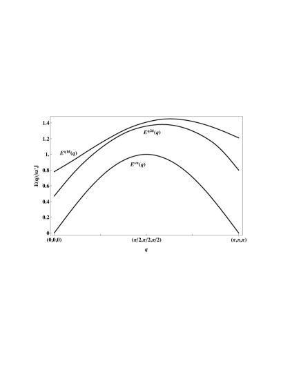
Figure 3: Similar to the earlier figures but for the quasi-1d and 2d systems of Eq. (24), with parameter $\xi=J_{\perp}/J=0.01$ for the quasi-1d spectrum $E^{\rm q1d}(q)$ and $\xi=10^{3}$ for the quasi-2d spectrum $E^{\rm q2d}(q)$. The spin-wave spectrum $E^{\rm sw}(q)$ is for the quasi-1d model.

where $\xi=J_{\perp}/J$. This is true also for the spin-wave spectrum $E^{\rm sw}(q)$ of Eq. (20). We notice that the spin-wave spectrum is gapless at zone boundaries, the longitudinal mode $E(q)$ of Eq. (9) however has nonzero gaps for any $\xi>0$, at which there is a long-range order ishi ; welz . In Fig. 3, we present our results for the spectrum, denoted as $E^{\rm q1d}(q)$, of the quasi-1d model with $A=1$ and $\xi=1.05$ as an example, together with the spin-wave spectrum $E^{\rm sw}(q)$. The gaps for $E^{\rm q1d}(q)$ at $q\to 0$ and ${\bf Q}=(\pi,\pi,\pi)$ are $0.78sz^{\prime}J$ and $1.21sz^{\prime}J$ respectively. Fig. 3 also includes our results for a quasi-2d model with $A=1$ and $1/\xi=J/J_{\perp}=10^{-3}$, denoted as $E^{\rm q2d}(q)$. The gap values for this quasi-2d spectrum at $q\to 0$ and ${\bf Q}=(\pi,\pi,\pi)$ are about $0.47sz^{\prime}J$ and $0.80sz^{\prime}J$ respectively. We also notice that at the particular two momenta $(\pi/2,\pi/2,0)$ and $(\pi,0,0)$, where the linear spin-wave spectrum has the same value of $sz^{\prime}J$ but the longitudinal mode has slightly different values, $1.36sz^{\prime}J$ and $1.41sz^{\prime}J$ respectively, due to magnon-magnon interactions as discussed earlier. This quasi-2d model may be relevant to the parent compounds of the high-$T_{c}$ cuprates, where the effective interlayer couplings $J/J_{\perp}$ between the CuO₂ planes are estimated to be between $10^{-2}$ and $10^{-5}$ sing .

IV.2 Quasi-1d model with KCuF₃ structure

In the experimentally well studied quasi-1d compound KCuF₃, the strong spin couplings along the chains are antiferromagnetic but the weak couplings on the basal plane are ferromagnetic. This compound can be described by the following Hamiltonian model,

$$H=J\sum_{l_{a},n_{1}}{\bf s}_{l_{a}}\cdot{\bf s}_{l_{a}+n_{1}}-\frac{J_{\perp}}{2}\left(\sum_{l_{a},n_{2}}{\bf s}_{l_{a}}\cdot{\bf s}_{l_{a}+n_{2}}+\sum_{l_{b},n_{2}}{\bf s}_{l_{b}}\cdot{\bf s}_{l_{b}+n_{2}}\right),$$ (26)

whose classical Néel state consists of two alternating planes, with all the spins on the $a$-plane pointing up and labeled by index $l_{a}$ and all the spins on the $b$-plane pointing down and labeled by index $l_{b}$. In Eq. (26), the nearest-neighbor indices $n_{1}$ and $n_{2}$ are as defined before with $n_{1}$ along the chains and $n_{2}$ on the basal planes, and both $J$ and $J_{\perp}>0$. The spin-wave spectrum is derived as

$$E^{\rm sw}(q)=2sJ\sqrt{\Delta^{2}_{q}-\cos^{2}q_{z}},$$ (27)

where $\Delta_{q}$ is defined as

$$\Delta_{q}=1+2\xi(1-\gamma_{q}^{\rm 2d}),\quad\xi=\frac{J_{\perp}}{J},$$ (28)

with $\gamma_{q}^{\rm 2d}=(\cos q_{x}+\cos q_{y})/2$. It is easy to check that when $J=0$, we recover the spin-wave spectrum of the 2d ferromagnetic model and that when $J_{\perp}=0$, we recover the spin-wave spectrum of the 1d antiferromagnetic model. For the longitudinal energy spectrum $E(q)$ of Eq. (9), the double commutator is now given by a different form as

$$N(q)=-J(1+\cos q_{z})\langle s^{+}_{l_{a}}s^{-}_{l_{a}+n_{1}}\rangle_{g}+2J_{\perp}(1-\gamma_{q}^{\rm 2d})\langle s^{+}_{l_{a}}s^{-}_{l_{a}+n_{2}}\rangle_{g},$$ (29)

and the structure factor $S(q)$ is as given before by Eqs. (6) and (13) in general forms and by Eqs. (17) and (18) in our approximation using the similar SWT ground state with the anisotropy parameter $A=1$. We notice that in Eq. (29), the two spin operators in the first correlation function $\langle s^{+}_{l_{a}}s^{-}_{l_{a}+n_{1}}\rangle_{g}$ are from the two sublattices respectively as before, but in the second correlation function $\langle s^{+}_{l_{a}}s^{-}_{l_{a}+n_{2}}\rangle_{g}$, they are from the same sublattice. So we still name the first one as before by $\tilde{g}_{1}=\langle s^{+}_{l_{a}}s^{-}_{l_{a}+n_{1}}\rangle_{g}/2s$ but the second one as $\tilde{g}^{\prime}_{1}=\langle s^{+}_{l_{a}}s^{-}_{l_{a}+n_{2}}\rangle_{g}/2s$. Using the similar SWT ground state, we obtain, for their Fourier transformations,

$$\tilde{g}_{q}=-\frac{1}{2}\frac{\cos q_{z}}{\sqrt{\Delta^{2}_{q}-\cos^{2}q_{z}}}$$ (30)

and

$$\tilde{g}^{\prime}_{q}=\rho_{q}=\frac{1}{2}\frac{\Delta_{q}}{\sqrt{\Delta^{2}_{q}-\cos^{2}q_{q}}}-\frac{1}{2},$$ (31)

respectively. We notice the quite different expressions for $\tilde{g}_{q}$ and $\tilde{g}^{\prime}_{q}$ as expected. We present our numerical results for $E(q)$ in Fig. 4, together with $E^{\rm sw}(q)$ of Eq. (27) for comparison, using the experimental values for the coupling constants, $J\approx 34$ meV, $J_{\perp}\approx 1.6$ meV and $s=1/2$ lake . Different to the longitudinal modes in other systems discussed earlier, we find that $E(q)$ has a smaller gap of about $0.63$J$\approx 21.4$ meV at AFWV ${\bf Q}=(0,0,\pi)$, and a larger gap of about $0.85$J$\approx 28.9$ meV at $q\to 0$. This gap value of $21.4$ meV at AFWV is about $40\%$ higher than the experimental value of about $15$ meV. The field theory by Essler et al. produces a gap value of about $17.4$ meV essl . However, there is uncertainty in the estimate value of the interchain coupling constant $J_{\perp}$. Lake et al. seem to have used the theoretical formula Eq. (56) in Ref. essl to obtain $J_{\perp}=1.6$ meV $=0.047J$. By different methods sati ; hira , $J_{\perp}$ was estimated to be $0.01J\sim 0.016J$. Using this estimate of $\xi=J_{\perp}/J=0.01$, we obtain the minimum gap value of $11.9$ meV at AFWV and $16.8$ meV at $q=0$. Naively, if we choose about the midpoint between the values of Refs. lake and sati , $J_{\perp}=0.85$ meV with $\xi\approx 0.025$, we obtain the minimum gap value of $0.49J=16.8$ meV at AFWV and $0.68J=23.2$ meV at $q=0$, in good agreement with the experiment for the minimum gap lake . Furthermore, with this value of $J_{\perp}=0.85$ meV, the linear spin-wave spectrum gap at ${\bf q}=(\pi,0,\pi)$ is $E^{\rm sw}(q)\approx 0.32J=10.9$ meV, very close to the gap value of $11\pm 0.5$ meV by the experiment sati . The longitudinal mode $E(q)$ is nearly flat in the region $(\eta,0,\pi)\sim(\eta,0,\pi)$ with $\pi\leq\eta\leq 0$, with the gap value about $0.59J=20.1$ meV at $(\pi,0,\pi)$. It will be very interesting indeed to compare with experimental results if available for the whole spectrum.

V summary and discussion

In summary, we have investigated the longitudinal excitations of various quantum antiferromagnets based on our recently proposed magnon-density-waves. Our numerical results show that the longitudinal mode always has a nonzero gap so long the system has a Néel-type long-range order and becomes gapless in in the limit of the 1d isotropic model. In particular, the spectrum of the longitudinal mode in our approximation is degenerate with the doublet spin-wave spectrum of SWT in the limit of the isotropic 1d model, in agreement with the triplet spin-wave spectrum of exact results for the spin-1/2 model by Bethe ansatz cloi . In the case of the simple cubic lattice model, the longitudinal mode with high energy values may not be well defined since there is little fluctuations in the nearly perfect classical long-range order. In the quasi-1d and quasi-2d models, where the quantum correction is large and the magnon density is significant, the magnon-density waves may be observable. Indeed, there are now ample evidence of the longitudinal modes in several quasi-1d systems as mentioned earlier in Sec. I. In particular, for the quasi-1d compound KCuF₃, our value for the minimum gap is in agreement with the experimental value lake . It will be interesting if more experimental results for the spectrum away from the minimum are available for comparison.

It is also interesting to note that the longitudinal modes were observed in the $ABX_{3}$-type antiferromagnets with both $s=1$ stei ; tun and $s=5/2$ harr ; kenz , clearly indicating that the modes are more general in their physics, independent of the mechanism which generates Haldane gap of the 1d model. The phenomenological field theory model with five fitting parameters employed by Affleck is derived from Haldane’s theory of the spin-1 chain affl . It will be interesting to apply our general microscopic analysis presented here to the $ABX_{3}$-type antiferromagnets where the basal plane is hexagonal and the corresponding Néel-like state has three sublattices rather than two sublattices discussed here. Other systems where we can apply our analysis for the magnon-density-waves include the quasi-2d systems where the next-nearest-neighbor antiferromagnetic couplings, in addition to the usual nearest-neighbor couplings, are present. These additional couplings cause quantum frustrations and the Néel-like order is further reduced hence greater the magnon density to support the magnon-density waves. Of particular current interest is the the parent compounds of the newly discovered high-$T_{c}$ superconducting ion-based pnictides where such next-nearest-couplings are believed to be significant ray .

Finally, we want to point out that there are two major approximations in our analysis here. The first is the linear operators $X_{q}$ employed in constructing the excitation states and the second is the SWT ground state $|\Psi_{\rm sw}\rangle$ employed in evaluating all the correlation functions involved. In regard to the first approximation, it is interesting to consider the case of the phonon-roton spectrum of the helium superfluid, where after inclusion of the nonlinear terms due to the couplings to the low-lying phonons (i.e., the so-called backflow correction), the values of the roton gap are reduced by about half to near the experimental values feyn ; jack . Clearly, the effects due to the couplings between the longitudinal modes and the gapless magnons in the antiferromagnetic systems also deserve further investigation. In regard to the second approximation, i.e., the SWT ground state employ in our calculations, improvement can be obtained by using better ground state functions available by more sophisticated microscopic many-body theories such as the coupled-cluster method ray2 ; yx2 and, particularly, its most recent extension where the strong correlations are included by a Jastrow correlation factor yx3 . We believe the quasi-1d and quasi-2d antiferromagnetic systems as studied here are good theoretical models from both the view point of the field theory approach which deal with most effectively the nonlinear effects of the 1d systems affl ; schu ; essl and of the microscopic many-body theory approach which provides general, systematic techniques in dealing with many-body correlations in plethora of quantum systems blai . The two theoretical approaches complement one another in study of these models and we wish to report our progress in these investigations in near future.

Figure 1: The energy spectrum $E(q)$ for the longitudinal mode of Eq. (9) for the square-lattice Heisenberg model of Eq. (10) with an anisotropy $A-1=1.5\times 10^{-4}$, together with the linear spin-wave spectrum $E^{\rm sw}(q)$ of Eq. (20) for comparison. This tiny anisotropy is a typical value for the parent compound of the high-$T_{c}$ superconducting cuprate, La₂CuO₄.

Figure 2: Similar to Fig. 1 but for the 1d model with the anisotropy $A=1.1$. In the isotropic limit of $A=1$, $E(q)$ approaches to $E^{\rm sw}(q)$, forming a triplet spectrum as described in details in text.

Figure 4: Similar to Fig. 3 but for the quasi-1d structure of KCuF₃ as described by Hamiltonian of Eq. (26), with parameter $\xi=J_{\perp}/J=1.6/34$ from the experiment lake . The spin-wave spectrum $E^{\rm sw}(q)$ is given by Eq. (27).

- (1) P.W. Anderson, Phys. Rev. 86, 694 (1952); T. Oguchi, ibid 117, 117 (1960); M. Takahashi, Phys. Rev. B 40, 2494 (1989).
- (2) See, for example, T. Huberman et al., Phys. Rev. B 72, 014413 (2005), and references therein.
- (3) J. des Cloizeaux and J.J. Pearson, Phys. Rev. 128, 2131 (1962); J.D. Johnson, S. Krinsky, and B.M. McCoy, Phys. Rev. A 8, 2526 (1973); L.D. Faddeev and L.A. Takhtajan, Phys. Lett. A 85, 375 (1981).
- (4) F.D.M. Haldane, Phys. Rev. Lett. 50, 1153 (1983).
- (5) D.A. Tennant et al., Phys. Rev. Lett. 70, 4003 (1993); Phys. Rev. B 52, 13368 (1995).
- (6) W.J.L. Buyers et al., Phys. Rev. Lett. 56, 371 (1986).
- (7) S. Shamoto et al., Phys. Rev. B 48, 13817 (1993); D. Munoz, I. deP.R. Moreira and F. Illas, Phys. Rev. B 71, 172505 (2005).
- (8) Y. Kamihara et al., J. Am. Chem. Soc. 130, 3296 (2008); C. de la Cruz et al., Nature 453, 899 (2008).
- (9) M. Steiner et al., J. Appl. Phys. 61, 3953 (1987).
- (10) Z. Tun, et al., Phys. Rev. B 42, 4677 (1990).
- (11) A. Harrison et al., Phys. Rev. B 43, 679 (1991).
- (12) M. Kenzelmann et al., Phys. Rev. B 66, 024407 (2002).
- (13) B. Lake, D.A. Tennant, and S.E. Nagler, Phys. Rev. B 71, 134412 (2005).
- (14) Ch. Rüegg et al., Phys. Rev. Lett. 100, 205701 (2008).
- (15) I. Affleck, Phys. Rev. Lett. 62, 474 (1989); I. Affleck and G.F. Wellman, Phys. Rev. B 46, 8934 (1992).
- (16) H.J. Schulz, Phys. Rev. lett. 77, 2790 (1996).
- (17) F.H.L. Essler, A.M. Tsvelik, and G. Delfino, Phys. Rev. B 56, 11001 (1997).
- (18) M.L. Plumer and A. Caillé, Phys. Rev. Lett. 68, 1042 (1992).
- (19) Y. Xian, Phys. Rev. B 74 212401 (2006); J. Phys.: Condens. Matter 19, 216221 (2007).
- (20) R.P. Feynman, Phys. Rev. 94, 262 (1954); R.P. Feynman and M. Cohen, ibid 102, 1189 (1956).
- (21) H.W. Jackson and E. Feenberg, Rev. Mod. Phys. 34, 686 (1962).
- (22) Y. Xian, in 150 years of Quantum Many-body Theories, ed. by R.F. Bishop, K.A. Gernoth, and N.R. Walet, World Scientific, Page 107, 2001; Y. Xian, Phys. Rev. B 66, 184427 (2002); Y. Xian, Phys. Rev. B 72, 224438 (2005).
- (23) The integrals over momentum space have bounds between as given by Eq. (19). In Ref. 19, the bounds of was used by mistake which makes no difference for most integrals but a small difference for integrals involving .
- (24) See, for example, B. Keimer et al., Phys. Rev. B 46, 14034 (1992).
- (25) Weihong Zheng, J. Oitmaa, and C.J. Hamer, Phys. Rev. B 71, 184440 (2005).
- (26) D. Welz, J. Phys.: Condens. Matter 5, 3643 (1993).
- (27) T. Ishikawa and T. Oguchi, Prog. Theo. Phys. 54, 1282 (1975).
- (28) R.P. Singh, Z.C. Tao and M. Singh, Phys. Rev. B 46, 1244 (1992).
- (29) See, for example, B. Schmidt, M Siahatgar, and P. Thalmeier, Phys. Rev. B 81, 165101 (2010), and references therein.
- (30) S.K. Satija et al. Phys. Rev. B 21, 2001 (1980).
- (31) K. Hirakawa and Y. Kurogi, Progr. Theor. Phys. S46, 147 (1970).
- (32) R.F. Bishop, R.G. Hale, and Y. Xian, Phys. Rev. Lett. 73, 3157 (1994); Chen Zeng, D.J.J. Farnell, and R.F. Bishop, J. Statist. Phys. 90, 327 (1998); D.J.J. Farnell and R.F. Bishop, in Quantum Magnetism (ed. U. Schollwöck, J. Richter, D.J.J. Farnell and R.F. Bishop), Lecture Notes in Physics, Vol. 645, Spinger-Verlag, Berlin, Page 307, 2004.
- (33) Y. Xian, Phys. Rev. A 77, 042103 (2008).
- (34) See, for example, J-P. Blaiza and G. Ripka, Quantum many-body theory of finite systems, MIT press, London, 1986.