Nonlinear behavior of geometric phases induced by photon pairs

Abstract

In this study, we observe the nonlinear behavior of the two-photon geometric phase for polarization states using time-correlated photons pairs. This phase manifests as a shift of two-photon interference fringes. Under certain arrangements, the geometric phase can vary nonlinearly and become very sensitive to a change in the polarization state. Moreover, it is known that the geometric phase for $N$ identically polarized photons is $N$ times larger than that for one photon. Thus, the geometric phase for two photons can become two times more sensitive to a state change. This high sensitivity to a change in the polarization can be exploited for precision measurement of small polarization variation. We evaluate the signal-to-noise ratio of the measurement scheme using the nonlinear behavior of the geometric phase under technical noise and highlight the practical advantages of this scheme.

I Introduction

When a system evolves in such a manner that it returns to its original state after some time, its wavefunction acquires an additional phase factor, which depends solely on the path traced in the ray space. The geometric phase was first discovered by Berry in adiabatic, cyclic evolution of pure quantum states  Berry (1984). The geometric phase has been generalized to other state evolutions including nonadiabatic evolution Aharonov and Anandan (1987); Anandan (1992), noncyclic evolution Samuel and Bhandari (1988); Morinaga et al. (2007) and mixed state evolutions  Uhlmann (1986); Sjöqvist et al. (2000). In optics, Pancharatnam reported the geometric phase in the polarization state Pancharatnam (1956). His pioneering work is now widely regarded as being an early precursor of the geometric phaseBerry (1987); Samuel and Bhandari (1988); Mukunda (1993).

There have been many interesting studies on the observation of the geometric phase Tomita and Chiao (1986); Simon et al. (1988); Chiao et al. (1988); Kwiat and Chiao (1991); Wagh and Rakhecha (1995a, b); Loredo et al. (2009); Kobayashi et al. (2011). Schmitzer et al. Schmitzer et al. (1993) reported that the variation of the geometric phase exhibits extraordinary nonlinearity associated with post-selection. In a certain arrangement, a small change in the pre- or post-selected state induces a large phase shift Schmitzer et al. (1993); Tewari et al. (1995); Bhandari (1997); Hils et al. (1999); Li et al. (1999); Tamate et al. (2009); Kobayashi et al. (2011). Several applications have been proposed that utilize the nonlinear behavior of the geometric phase including optical switching Tewari et al. (1995); Schmitzer et al. (1991) and high-precision measurements Hils et al. (1999); Tamate et al. (2009).

Another important topic is the manifestation of the geometric phase in bipartite and multipartite systems. Klyshko Klyshko (1989) showed that the geometric phase for $N$ identically polarized photons is $N$ times that for one photon. This principle has been observed for two photons in a two-photon interference experiment utilizing time-correlated photon pairs Brendel et al. (1995). The effect of entanglement on the geometric phase has also been discussed in  Sjöqvist (2000); Hessmo and Sjöqvist (2000); Ge and Wadati (2005); Williamson and Vedral (2007).

The aim of the present study is to observe the nonlinear behavior of the geometric phases of two photons. To the best of our knowledge, this is the first observation of the nonlinear behavior of the two-photon geometric phase. In our experiment, time-correlated photon pairs with the same polarization are incident on a Mach-Zehnder interferometer with polarization elements. We can observe the geometric phase of two photons as the phase shift of two-photon interference fringes using coincidence counting. This phase shift is two times larger than that for one photon. It lies between $0$ and $4\pi$, i.e., the two-photon interference fringe can be shifted by up to two fringe periods. Moreover, the nonlinear behavior suggests that the geometric phase for two photons is two times more sensitive to a change in the input polarization than the one-photon case. A minute change in the input polarization results in a large shift in the two-photon interference fringe.

This high sensitivity to the input polarization can be utilized to precisely measure small variations. We show that the signal-to-noise ratio (SNR) of the measurement scheme using the geometric phase for multiphoton can be improved for a certain type of noise. Recently, there has been a related discussion about signal enhancement with post-selection, the so-called weak measurement amplification, in the presence of some noises  Aharonov et al. (1988); Hosten and Kwiat (2008); Dixon et al. (2009); Starling et al. (2009); Feizpour et al. (2010).

The remainder of this paper is organized as follows. In Sec. II, we briefly review the geometric phase induced by a change in the polarization state in a one-photon interferometer and we show that the geometric phase can be very sensitive to a change in the polarization state for a certain arrangement. Moreover, we show that the $N$-fold geometric phase for $N$ identically polarized photons can be observed using the same interferometer. In Sec. III, we introduce the experimental setup used to observe the geometric phase for two photons and the results indicating the twofold geometric phase and its nonlinearity. In Sec. IV, we consider the application of the nonlinear behavior of geometric phases to high-precision measurements. The SNR is evaluated for a practical situation that includes both shot and technical noise. A summary is presented in Sec. V.

II Geometric phase for $N$ photons and its nonlinearity

II.1 Geometric phases in a one-photon interferometer

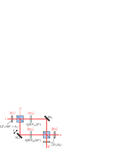
Figure 1: (Color online) A Mach-Zehnder interferometer with polarization elements used to observe the geometric phase. The interferometer contains two linear polarizers, LP₁ and LP₂, and two quarter-wave plates, QWP${}_{\scriptsize\mbox{A}}$ and QWP${}_{\scriptsize\mbox{B}}$. The angles of the transmission axes of LP₁ and LP₂ are respectively $90\mbox{${}^{\circ}$}+\theta_{1}$ and $\theta_{2}$, and those of the fast axes of QWP${}_{\scriptsize\mbox{A}}$ and QWP${}_{\scriptsize\mbox{B}}$ are $0^{\circ}$ and $90^{\circ}$. The states $|\mbox{$\psi_{1}$}\rangle$, $|\mbox{$\psi_{2}$}\rangle$, $|\mbox{$\psi_{\scriptsize\mbox{A}}$}\rangle$, and $|\mbox{$\psi_{\scriptsize\mbox{B}}$}\rangle$ are the polarization states after LP₁, LP₂, QWP${}_{\scriptsize\mbox{A}}$, and QWP${}_{\scriptsize\mbox{B}}$, respectively.

We begin by reviewing the geometric phase induced by changing the polarization state in one-photon interferometer. Consider a Mach-Zehnder interferometer with polarization elements as shown in Fig. 1. In each arm of the interferometer, the initial polarization state $|\mbox{$\psi_{1}$}\rangle$ of an incident photon is converted into new polarization states $|\mbox{$\psi_{\scriptsize\mbox{A}}$}\rangle$ and $|\mbox{$\psi_{\scriptsize\mbox{B}}$}\rangle$. If an additional U(1) phase shift $\chi$ is introduced in one of the arms, the output intensity $I_{\scriptsize\mbox{m}}$ will be

$$I_{\scriptsize\mbox{m}} \propto\left\||\mbox{$\psi_{\scriptsize\mbox{A}}$}\rangle+{\mathrm{e}}^{{\mathrm{i}}\chi}|\mbox{$\psi_{\scriptsize\mbox{B}}$}\rangle\right\|^{2}$$ (1)

$$=2\left[1+v_{\scriptsize\mbox{m}}\cos(\chi-\phi_{\scriptsize\mbox{m}})\right],$$ (2)

where the visibility $v_{\scriptsize\mbox{m}}$ and the phase shift $\phi_{\scriptsize\mbox{m}}$ are respectively given by

$$v_{\scriptsize\mbox{m}} =\left|\langle\mbox{$\psi_{\scriptsize\mbox{B}}$}|\mbox{$\psi_{\scriptsize\mbox{A}}$}\rangle\right|,$$ (3)

$$\phi_{\scriptsize\mbox{m}} =\arg\langle\mbox{$\psi_{\scriptsize\mbox{B}}$}|\mbox{$\psi_{\scriptsize\mbox{A}}$}\rangle.$$ (4)

The phase shift $\phi_{\scriptsize\mbox{m}}$ expresses the phase difference between the two different polarization states and is called the relative phase Pancharatnam (1956). When $\langle\mbox{$\psi_{\scriptsize\mbox{A}}$}|\mbox{$\psi_{\scriptsize\mbox{B}}$}\rangle=0$, two states can be perfectly distinguished and the path followed by the photon is unambiguously discriminated. The interference is then completely destroyed and the visibility $v_{\scriptsize\mbox{m}}$ is reduced to zero.

Next, we consider the phase shift induced by post-selection. Post-selection of the polarization state into $|\mbox{$\psi_{2}$}\rangle$ causes the output intensity $I_{\scriptsize\mbox{f}}$ to become

$$I_{\scriptsize\mbox{f}} \propto\left\|\left(c_{\scriptsize\mbox{A}}+{\mathrm{e}}^{{\mathrm{i}}\chi}c_{\scriptsize\mbox{B}}\right)|\mbox{$\psi_{2}$}\rangle\right\|^{2}$$ (5)

$$=2p\left[1+v_{\scriptsize\mbox{f}}\cos\left(\chi-\phi_{\scriptsize\mbox{f}}\right)\right],$$ (6)

where $c_{\scriptsize\mbox{A}}=\langle\mbox{$\psi_{2}$}|\mbox{$\psi_{\scriptsize\mbox{A}}$}\rangle$ and $c_{\scriptsize\mbox{B}}=\langle\mbox{$\psi_{2}$}|\mbox{$\psi_{\scriptsize\mbox{B}}$}\rangle$. The success probability $p$ of the post-selection, the visibility $v_{\scriptsize\mbox{f}}$, and the phase shift $\phi_{\scriptsize\mbox{f}}$ are expressed as

$$p =\frac{1}{2}\left(|c_{\scriptsize\mbox{A}}|^{2}+|c_{\scriptsize\mbox{B}}|^{2}\right),$$ (7)

$$v_{\scriptsize\mbox{f}} =\frac{2|c_{\scriptsize\mbox{A}}c_{\scriptsize\mbox{B}}|}{|c_{\scriptsize\mbox{A}}|^{2}+|c_{\scriptsize\mbox{B}}|^{2}},$$ (8)

$$\phi_{\scriptsize\mbox{f}} =\arg\langle\mbox{$\psi_{\scriptsize\mbox{B}}$}|\mbox{$\psi_{2}$}\rangle\langle\mbox{$\psi_{2}$}|\mbox{$\psi_{\scriptsize\mbox{A}}$}\rangle,$$ (9)

respectively. Equation (8) shows that even when $|\mbox{$\psi_{\scriptsize\mbox{A}}$}\rangle$ is orthogonal to $|\mbox{$\psi_{\scriptsize\mbox{B}}$}\rangle$, the visibility is completely recovered ($v_{\scriptsize\mbox{f}}=1$) provided $|c_{\scriptsize\mbox{A}}|=|c_{\scriptsize\mbox{B}}|$. In this condition, $|\mbox{$\psi_{\scriptsize\mbox{A}}$}\rangle$ and $|\mbox{$\psi_{\scriptsize\mbox{B}}$}\rangle$ are projected into the same polarization state $|\mbox{$\psi_{2}$}\rangle$ with the same probability, and it is not possible to determine the photon paths. This shows that post-selection completely erases the which-path information and recovers the interference.

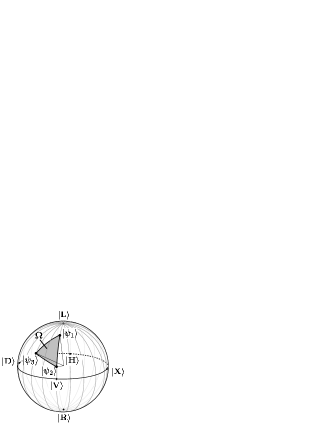
Figure 2: Spherical triangle on the Poincaré sphere formed by three polarization states, $|\mbox{$\psi_{1}$}\rangle$, $|\mbox{$\psi_{2}$}\rangle$, and $|\mbox{$\psi_{3}$}\rangle$. The geometric phase is proportional to the solid angle $\Omega$ of the spherical triangle. The poles correspond to the right and left circular polarization states, $|\mbox{${\mu\Omega\mathrm{R}}$}\rangle$ and $|\mbox{${\mu\Omega\mathrm{L}}$}\rangle$, and the equator corresponds to the linear polarization states; for example, the horizontal polarization $|\mbox{${\mu\Omega\mathrm{H}}$}\rangle$, vertical polarization $|\mbox{${\mu\Omega\mathrm{V}}$}\rangle$, $45^{\circ}$ polarization $|\mbox{${\mu\Omega\mathrm{D}}$}\rangle$, and $135^{\circ}$ polarization $|\mbox{${\mu\Omega\mathrm{X}}$}\rangle$.

The net phase shift induced by the post-selection is calculated as

$$\gamma(\psi_{\scriptsize\mbox{A}},\psi_{\scriptsize\mbox{B}},\psi_{2}) \equiv\phi_{\scriptsize\mbox{f}}-\phi_{\scriptsize\mbox{m}}$$ (10)

$$=\arg\langle\mbox{$\psi_{\scriptsize\mbox{A}}$}|\mbox{$\psi_{\scriptsize\mbox{B}}$}\rangle\langle\mbox{$\psi_{\scriptsize\mbox{B}}$}|\mbox{$\psi_{2}$}\rangle\langle\mbox{$\psi_{2}$}|\mbox{$\psi_{\scriptsize\mbox{A}}$}\rangle.$$ (11)

The cyclic form on the right-hand side of Eq. (11) is gauge invariant (i.e., independent of the choice of the phase factor of each state) because the bra and ket vectors for each state appear pairwise. This phase shift $\gamma$ is the geometric phase Pancharatnam (1956) and can be interpreted geometrically on the Poincaré sphere as shown in Fig. 2. The geometric phase $\gamma(\psi_{1},\psi_{2},\psi_{3})$ can be shown to be proportional to the solid angle $\Omega(\psi_{1},\psi_{2},\psi_{3})$ of the spherical triangle connecting the states $|\mbox{$\psi_{1}$}\rangle$, $|\mbox{$\psi_{2}$}\rangle$, and $|\mbox{$\psi_{3}$}\rangle$ with geodesic arcs on the Poincaré sphere Pancharatnam (1956); Aravind (1992), i.e.,

$$\gamma(\psi_{1},\psi_{2},\psi_{3})=\frac{1}{2}\Omega(\psi_{1},\psi_{2},\psi_{3}).$$ (12)

The sign of the geometric phase is determined by the order of the states.

II.2 Nonlinearity of geometric phase for one photon

Here, we consider the nonlinear behavior of the geometric phase for one photon using the experimental setup shown in Fig. 1. This is a similar setup to the one used in previous experiments with a laser light source  Li et al. (1999); Kobayashi et al. (2011).

The initial polarization state $|\mbox{$\psi_{1}$}\rangle$ is prepared by the linear polarizer LP₁:

$$|\mbox{$\psi_{1}$}\rangle =-\sin\theta_{1}|\mbox{$\text{H}$}\rangle+\cos\theta_{1}|\mbox{$\text{V}$}\rangle,$$ (13)

where $\theta_{1}$ is the angle between the vertical line ($-\pi/2\leq\theta_{1}\leq\pi/2$) and the transmission axis of LP₁, $|\mbox{$\text{H}$}\rangle$ is the horizontal polarization state, and $|\mbox{$\text{V}$}\rangle$ is the vertical polarization state. The initial state $|\mbox{$\psi_{1}$}\rangle$ is changed by two quarter-wave plates, QWP${}_{\scriptsize\mbox{A}}$ and QWP${}_{\scriptsize\mbox{B}}$, whose fast axes are aligned to form angles of $0\mbox{${}^{\circ}$}$ and $90\mbox{${}^{\circ}$}$:

$$|\mbox{$\psi_{\scriptsize\mbox{A}}$}\rangle =-\sin\theta_{1}|\mbox{$\text{H}$}\rangle+{\mathrm{i}}\cos\theta_{1}|\mbox{$\text{V}$}\rangle,$$ (14)

$$|\mbox{$\psi_{\scriptsize\mbox{B}}$}\rangle =-{\mathrm{i}}\sin\theta_{1}|\mbox{$\text{H}$}\rangle+\cos\theta_{1}|\mbox{$\text{V}$}\rangle.$$ (15)

Finally, these polarization states are projected into the same state $|\mbox{$\psi_{2}$}\rangle$ by the linear polarizer LP₂:

$$|\mbox{$\psi_{2}$}\rangle=\cos\theta_{2}|\mbox{$\text{H}$}\rangle+\sin\theta_{2}|\mbox{$\text{V}$}\rangle,$$ (16)

where $\theta_{2}$ is the angle between the horizontal line ($0\leq\theta_{2}\leq\pi$) and the transmission axis of LP₂. Since this setup satisfies $|\langle\mbox{$\psi_{2}$}|\mbox{$\psi_{\scriptsize\mbox{A}}$}\rangle|=|\langle\mbox{$\psi_{2}$}|\mbox{$\psi_{\scriptsize\mbox{B}}$}\rangle|$, the visibility of the interference fringe $v_{\scriptsize\mbox{f}}$ becomes unity.

(a)     One photon

(b)     Two photons

Figure 3: Geometric phases and success probabilities of post-selection for (a) one and (b) two photons. The first row shows the variation of the geometric phase and the second row shows the success probability of the post-selection with respect to $\theta_{1}$ for $\theta_{2}=\pi/50$ (solid line), $\theta_{2}=\pi/10$ (dashed line), and $\theta_{2}=\pi/4$ (dotted line).

Substituting Eqs. (14) – (16) into Eqs. (4) and (11), we can obtain the relative phase $\phi_{\scriptsize\mbox{m}}$ and the geometric phase $\gamma(\psi_{\scriptsize\mbox{A}},\psi_{\scriptsize\mbox{B}},\psi_{2})$:

$$\phi_{\scriptsize\mbox{m}} =\begin{cases}\displaystyle\frac{\pi}{2}\hskip 22.76228pt(\cos 2\theta_{1}\geq 0),\\ \vspace*{-0.3cm}\\ \displaystyle-\frac{\pi}{2}\hskip 14.22636pt(\cos 2\theta_{1}<0),\end{cases}$$ (17)

$$\gamma =\begin{cases}&\displaystyle 2\tan^{-1}\left(\frac{\tan\theta_{1}}{\tan\theta_{2}}\right)\hskip 22.76228pt(\cos 2\theta_{1}\geq 0),\\ \vspace*{-0.3cm}\\ &\displaystyle 2\tan^{-1}\left(\frac{\tan\theta_{1}}{\tan\theta_{2}}\right)+\pi\hskip 5.12128pt(\cos 2\theta_{1}<0),\end{cases}$$ (18)

where the range of $\tan^{-1}()$ is $(-\pi/2:\pi/2]$. The summation of two phases is given by

$$\phi_{\scriptsize\mbox{f}}=\phi_{\scriptsize\mbox{m}}+\gamma=2\tan^{-1}\left(\frac{\tan\theta_{1}}{\tan\theta_{2}}\right)+\frac{\pi}{2}.$$ (19)

The top of Fig. 3(a) shows the variation of Eq. (18) with respect to $\theta_{1}$ for three different values of $\theta_{2}$. It shows that, except for $\theta_{2}=\pi/4$, the geometric phase is nonlinear with respect to $\theta_{1}$. The phase shift around $\theta_{1}=0$ is sensitive to a change in $\theta_{1}$ when $\theta_{2}$ is small. This nonlinear variation can be observed as a rapid displacement in the interference fringe when we change $\theta_{1}$ by rotating LP₁  Schmitzer et al. (1993); Tewari et al. (1995); Bhandari (1997); Hils et al. (1999); Li et al. (1999).

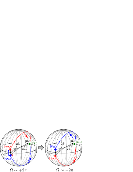
Figure 4: (Color online) Geometrical interpretation of the nonlinear variation of the geometric phase around $(\theta_{1},\theta_{2})=(0,0)$. If $|\mbox{$\psi_{\scriptsize\mbox{A}}$}\rangle$ and $|\mbox{$\psi_{\scriptsize\mbox{B}}$}\rangle$ are close to each other across the vertical polarization state $|\mbox{$\text{V}$}\rangle$ on the Poincaré sphere, the area of the spherical triangle will vary rapidly with movement of $|\mbox{$\psi_{\scriptsize\mbox{A}}$}\rangle$ and $|\mbox{$\psi_{\scriptsize\mbox{B}}$}\rangle$.

Equation (18) shows that the nonlinear behavior of the phase shift originates from the geometric phase $\gamma$ and can be understood intuitively in terms of the geometry on the Poincaré sphere. In the present setup, $|\mbox{$\psi_{\scriptsize\mbox{A}}$}\rangle$ and $|\mbox{$\psi_{\scriptsize\mbox{B}}$}\rangle$ given by Eqs. (13) and (15) can be depicted at a latitude of $\pm 2\theta_{1}$ on the prime meridian and the final state $|\mbox{$\psi_{2}$}\rangle$ given by Eq. (16) can be depicted on the equator at a longitude of $2\theta_{2}$ (see Fig. 4). When $0<\theta_{2}<\theta_{1}\ll 1$, $|\mbox{$\psi_{\scriptsize\mbox{A}}$}\rangle$ and $|\mbox{$\psi_{\scriptsize\mbox{B}}$}\rangle$ are located near the vertical polarization state while $|\mbox{$\psi_{2}$}\rangle$ is near the horizontal polarization state. In this condition, the spherical triangle connecting $|\mbox{$\psi_{\scriptsize\mbox{A}}$}\rangle$, $|\mbox{$\psi_{\scriptsize\mbox{B}}$}\rangle$, and $|\mbox{$\psi_{2}$}\rangle$ almost degenerates to a great circle. Therefore, the solid angle $\Omega$ is almost equal to $+2\pi$. Now, we consider that $\theta_{1}$ is changed to exchange the positions of $|\mbox{$\psi_{\scriptsize\mbox{A}}$}\rangle$ and $|\mbox{$\psi_{\scriptsize\mbox{B}}$}\rangle$ on the Poincaré sphere. $|\mbox{$\psi_{\scriptsize\mbox{A}}$}\rangle$ and $|\mbox{$\psi_{\scriptsize\mbox{B}}$}\rangle$ move toward $|\mbox{$V$}\rangle$ with decreasing $\theta_{1}$. When the distance between $|\mbox{$\psi_{\scriptsize\mbox{A}}$}\rangle$ and $|\mbox{$\psi_{\scriptsize\mbox{B}}$}\rangle$ becomes less than $2\theta_{2}$, the area of the spherical triangle shrinks rapidly. After traversing $|\mbox{$\text{V}$}\rangle$, the area $\Omega$ blows up rapidly and approaches $-2\pi$. Thus, the area $\Omega$ changes rapidly from $-2\pi$ to $2\pi$ around $\theta_{1}=0$ and the phase shift can vary nonlinearly.

In the nonlinear region of the phase shift around $\theta_{1}=0$, the success probability of the post-selection drops according to Eq. (7):

$$p(\theta_{1},\theta_{2}) =\sin^{2}\theta_{1}\cos^{2}\theta_{2}+\cos^{2}\theta_{1}\sin^{2}\theta_{2}.$$ (20)

The bottom of Fig. 3(a) shows a plot of Eq. (20) on a logarithmic scale. It implies that a rapid change in the geometric phase around $\theta_{1}=0$ can be achieved at the expense of the output intensity.

II.3 Geometric phase for $N$ photons

As shown by Klyshko Klyshko (1989), $N$ identically polarized photons are expected to acquire $N$ times the geometric phase for one photon. In this section, we theoretically analyze the interferometric method for observing the $N$-fold geometric phase.

Assuming that a collection of $N$ photons is incident on the interferometer (see Fig. 1) and that these photons can form path-entangled states in the interferometer known as $N00N$ states (i.e., all the $N$ photons pass through path A or path B  Sanders (1989); Bollinger et al. (1996); Boto et al. (2000); Edamatsu et al. (2002); Walther et al. (2004); Nagata et al. (2007); Dowling (2008)), the polarization state of the $N$ photons can be expressed as the $N$th tensor product:

$$|\mbox{$\Psi_{i}$}\rangle\equiv|\mbox{$\psi_{i}$}\rangle^{\otimes N},$$ (21)

where $i=(1,2,\text{A},\text{B})$ and $\otimes$ represents the tensor product.

If an additional U(1) phase shift $\chi$ is introduced in one of the arms, the output intensity $I_{\scriptsize\mbox{m}}$ measured by the $N$-photon coincidence detector will be

$$I_{\scriptsize\mbox{m}} \propto\left\||\mbox{$\Psi_{\scriptsize\mbox{A}}$}\rangle+{\mathrm{e}}^{{\mathrm{i}}N\chi}|\mbox{$\Psi_{\scriptsize\mbox{B}}$}\rangle\right\|^{2}$$ (22)

$$=2\left[1+V_{\scriptsize\mbox{m}}\cos\left(N\chi-\Phi_{\scriptsize\mbox{m}}\right)\right],$$ (23)

where the visibility $V_{\scriptsize\mbox{m}}$ and the phase shift $\Phi_{\scriptsize\mbox{m}}$ are respectively given by

$$V_{\scriptsize\mbox{m}} =|\langle\mbox{$\psi_{\scriptsize\mbox{B}}$}|\mbox{$\psi_{\scriptsize\mbox{A}}$}\rangle|^{N},$$ (24)

$$\Phi_{\scriptsize\mbox{m}} =N\arg\langle\mbox{$\psi_{\scriptsize\mbox{B}}$}|\mbox{$\psi_{\scriptsize\mbox{A}}$}\rangle.$$ (25)

Since $N$ photons act as a collective entity in the interferometer, the phase term in Eq. (23) is $N$ times that for the one photon case.

After post-selection into the polarization state $|\mbox{$\Psi_{2}$}\rangle$, the output intensity $I_{\scriptsize\mbox{f}}$ is given by

$$I_{\scriptsize\mbox{f}} \propto\left\|\left(\langle\mbox{$\Psi_{2}$}|\mbox{$\Psi_{\scriptsize\mbox{A}}$}\rangle+{\mathrm{e}}^{{\mathrm{i}}N\chi}\langle\mbox{$\Psi_{2}$}|\mbox{$\Psi_{\scriptsize\mbox{B}}$}\rangle\right)|\mbox{$\Psi_{2}$}\rangle\right\|^{2}$$ (26)

$$=2P\left[1+V_{\scriptsize\mbox{f}}\cos\left(N\chi-\Phi_{\scriptsize\mbox{f}}\right)\right],$$ (27)

where the success probability for post-selection $P$, the visibility $V_{\scriptsize\mbox{f}}$, and the phase shift $\Phi_{\scriptsize\mbox{f}}$ are respectively expressed by

$$P =\frac{1}{2}\left(|c_{\scriptsize\mbox{A}}|^{2N}+|c_{\scriptsize\mbox{B}}|^{2N}\right),$$ (28)

$$V_{\scriptsize\mbox{f}} =\frac{2|c_{\scriptsize\mbox{A}}c_{\scriptsize\mbox{B}}|^{N}}{|c_{\scriptsize\mbox{A}}|^{2N}+|c_{\scriptsize\mbox{B}}|^{2N}}$$ (29)

$$\Phi_{\scriptsize\mbox{f}} =N\arg\langle\mbox{$\psi_{\scriptsize\mbox{B}}$}|\mbox{$\psi_{2}$}\rangle\langle\mbox{$\psi_{2}$}|\mbox{$\psi_{\scriptsize\mbox{A}}$}\rangle.$$ (30)

Substituting Eqs. (14) – (16) into Eqs. (28) – (30) we can obtain

$$P =\left(\sin^{2}\theta_{1}\cos^{2}\theta_{2}+\cos^{2}\theta_{1}\sin^{2}\theta_{2}\right)^{N},$$ (31)

$$V_{\scriptsize\mbox{f}} =1,$$ (32)

$$\Phi_{\scriptsize\mbox{f}} =2N\tan^{-1}\left(\frac{\tan\theta_{1}}{\tan\theta_{2}}\right)+\frac{N\pi}{2}.$$ (33)

Figure 3(b) shows the variation of $P$ and $\Phi_{\scriptsize\mbox{f}}$ with respect to $\theta_{1}$ for $N=2$.

Since the slope of the phase shift for $N$ photons around $\theta_{1}=0$ is $N$ times steeper than that for one photon, we can obtain an $N$-fold enhancement in the variation of $\theta_{1}$ [see the top of Fig. 3]. However, the success probability of post-selection $P$ decreases as the $N$th power of the one-photon success probability $p$ because $P$ corresponds to the probability that all $N$ photons are successfully post-selected into state $|\mbox{$\psi_{2}$}\rangle$ [see the bottom of Fig. 3].

III Observation of geometric phase for two photons using photon pairs

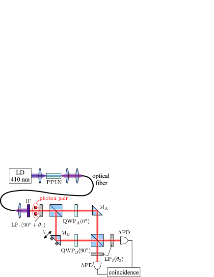
Figure 5: (Color online) Experimental setup for observing the geometric phase for two photons. IF is an interference filter and M${}_{\scriptsize\mbox{A}}$ and M${}_{\scriptsize\mbox{B}}$ are total reflection mirrors.

III.1 Two-photon interference in Mach-Zehnder interferometer

We consider a two-photon state input at port 1 and a vacuum state input at port $1^{\prime}$ of a symmetric Mach-Zehnder interferometer. The first beam splitter splits the incident photons into two paths A and B:

$$|\mbox{$2$}\rangle_{1}|\mbox{$0$}\rangle_{1^{\prime}}$$

$$\rightarrow |\mbox{$2$}\rangle_{\scriptsize\mbox{A}}|\mbox{$0$}\rangle_{\scriptsize\mbox{B}}+{\mathrm{e}}^{{\mathrm{i}}2\chi}|\mbox{$0$}\rangle_{\scriptsize\mbox{A}}|\mbox{$2$}\rangle_{\scriptsize\mbox{B}}+2{\mathrm{e}}^{{\mathrm{i}}\chi}|\mbox{$1$}\rangle_{\scriptsize\mbox{A}}|\mbox{$1$}\rangle_{\scriptsize\mbox{B}},$$ (34)

where the photon number state with $N$ photons in path (or port) $p$ is written as $|\mbox{$N$}\rangle_{p}$ and $\chi$ is the additional phase shift. When we operate coincidence counting between output port $2$ and $2^{\prime}$, the $|\mbox{$1$}\rangle_{\scriptsize\mbox{A}}|\mbox{$1$}\rangle_{\scriptsize\mbox{B}}$ term in Eq. (34) is missing due to the complete destructive two-photon interference Hong et al. (1987), producing a two-photon path-entangled state to be detected.

The above consideration is valid even if the interferometer contains polarization elements as shown in Fig. 1 because the polarization states of two photons are eventually projected into the same states with the same probability at output ports $2$ and $2^{\prime}$. Hence, we can observe the nonlinear behavior of the phase shift of two photons using coincidence counting between output ports $2$ and $2^{\prime}$.

III.2 Experimental setup

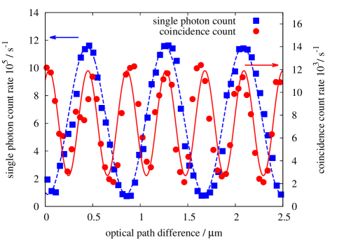
Figure 6: (Color online) Measured one- and two-photon interference fringes. The blue squares ($\blacksquare$) and red circles ($\bullet$) indicate the one-photon interference measured by single-photon counting and the two-photon interference measured by coincidence counting, respectively. The solid curves show the theoretical interferences.

(a)     One photon

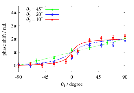
(b)     Two photons

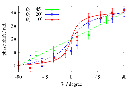
Figure 7: (Color online) Experimental results for geometric phases of (a) one and (b) two photons with respect to $\theta_{1}$ for three different values of $\theta_{2}$.

Fig. 5 shows a schematic representation of the experimental setup. Photon pairs are generated in the periodically poled LiNbO₃ (PPLN) waveguide via degenerate type-I parametric down-conversion of a 410-nm blue light from a laser diode (LD). The temperature of PPLN is calibrated by a temperature controller to satisfy the phase matching condition. The center wavelength of the photon pairs is $820$ ${\mu\Omega\mathrm{nm}}$ and its spectral bandwidth is restricted to $20$ ${\mu\Omega\mathrm{nm}}$ by the interference filter IF. After beam shaping by the single-mode optical fiber, photon pairs traverse the Mach-Zehnder interferometer with polarization elements. The phase difference between two arms is varied continuously by shifting the total reflection mirror M${}_{\scriptsize\mbox{B}}$ using a piezoelectric translation stage. The outputs of the interferometer are coupled to a pair of single-photon counting modules (Perkin Elmer, SPCM-AQR-14). Individual photon counts and coincidence counts are recorded using field-programmable gate array (FPGA) electronics connected to a personal computer Branning et al. (2009).

III.3 Observation of geometric phases for one and two photons

Figure 6 shows the one- and two-photon interference fringes obtained for photon pairs. The solid line is a fit by a sinusoidal function. The vertical axis shows the single-photon and the coincidence count rates. This figure shows that the two-photon interference fringe has a period given by the wavelength of the pump light and an average visibility of $63\%$.

Figure 7 shows the phase shifts of one-photon and two-photon interference fringes with respect to $\theta_{1}$ for $\theta_{2}=45\mbox{${}^{\circ}$}$ (filled green circles), $20\mbox{${}^{\circ}$}$ (open blue circles), and $10\mbox{${}^{\circ}$}$ (filled red squares). The origin of the vertical axis is determined by the position of fringes when $\theta_{1}=-90\mbox{${}^{\circ}$}$ and the value of the vertical axis shows the displacement of fringes normalized by one period of the fringes. The solid line in Fig. 7 indicates the theoretical curve calculated from Eq. (33). For both one- and two-photon interference, the gradient of the variation of the phase shift around $\theta_{1}=0\mbox{${}^{\circ}$}$ increases with decreasing $\theta_{2}$. This implies that the variation in the phase shift becomes more sensitive to a variation in $\theta_{1}$. Moreover, the phase shift for two photons is two times larger than that for one photon. Thus, the gradient of the phase shift for two photons around $\theta_{1}=0\mbox{${}^{\circ}$}$ also becomes two times steeper than that for one photon.

IV Discussion : SNR of measurement scheme using nonlinear behavior of geometric phase

In what follows, we consider the measurement of a small polarizer angle $\theta_{1}$ ($|\theta_{1}|\ll 1$) through the phase shift of the interference fringes. As shown in the previous section, the geometric phase becomes sensitive to a variation in $\theta_{1}$ around $\theta_{1}=0$ when $\theta_{2}$ is small. Moreover, the geometric phase for $N$ photons will be $N$ times more sensitive to a variation in $\theta_{1}$. Utilizing this nonlinear behavior, we can measure the small angle $\theta_{1}$ from the large phase shift of the ($N$-photon) interference fringe. However, the small success probability of post-selection around $\theta_{1}=0$ might cancel out the advantage of the large phase shift.

In this section, we calculate the SNR of this measurement using the geometric phase for $N$ photons to evaluate its advantages and disadvantages. Interferometric phase measurement is subject to various noises. In the ideal situation, the shot noise is dominant, whereas in most experiments, the SNR is limited by technical noises such as excessive fluctuations in the light sources. Thus, we calculate the SNR for a case with technical noise in addition to the shot noise. We show that the nonlinearity of the geometric phase does not improve the SNR in the shot noise limit. However, under certain technical noises, the large phase shift due to the nonlinearity of the geometric phase can be of practical advantage.

IV.1 SNR of direct measurement

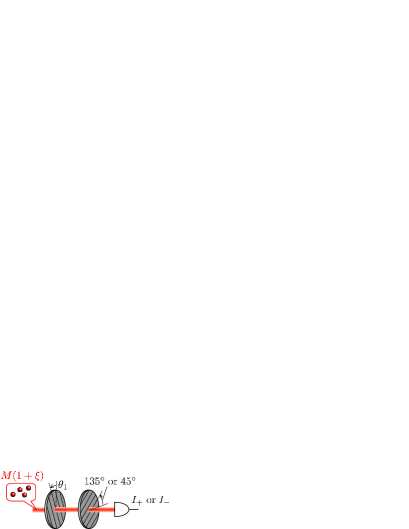
Figure 8: (Color online) Direct measurement of $\theta_{1}$. $I_{+}$ and $I_{-}$ show the single photon counts for $135\mbox{${}^{\circ}$}$ and $45\mbox{${}^{\circ}$}$ polarization, respectively.

First, we evaluate the SNR of the direct measurement of $\theta_{1}$ without utilizing the geometric phase as shown in Fig. 8. We consider a sequential measurement of single-photon counts integrated over the interval $\tau$ for $45\mbox{${}^{\circ}$}$ and $135\mbox{${}^{\circ}$}$ polarizations expressed as

$$\langle\mbox{$I_{+}(\tau)$}\rangle =\eta\tau M|\langle\mbox{$\text{X}$}|\mbox{$\psi_{1}$}\rangle|^{2}=\frac{\eta\tau M}{2}\left(1+\sin 2\theta_{1}\right),$$ (35)

$$\langle\mbox{$I_{-}(\tau)$}\rangle =\eta\tau M|\langle\mbox{$\text{D}$}|\mbox{$\psi_{1}$}\rangle|^{2}=\frac{\eta\tau M}{2}\left(1-\sin 2\theta_{1}\right),$$ (36)

where $\langle\mbox{$\hskip 2.84544pt\cdot\hskip 2.84544pt$}\rangle$ shows the ensemble mean value, $M$ is the number of incident photons per unit time, and $\eta$ is the detection efficiency. The angle $\theta_{1}$ can be measured from the ratio of the difference to the sum between $\langle\mbox{$I_{+}$}\rangle$ and $\langle\mbox{$I_{-}$}\rangle$:

$$\langle\mbox{$n(\theta_{1})$}\rangle \equiv\frac{\langle\mbox{$I_{+}(\tau)$}\rangle-\langle\mbox{$I_{-}(\tau)$}\rangle}{\langle\mbox{$I_{+}(\tau)$}\rangle+\langle\mbox{$I_{-}(\tau)$}\rangle}$$ (37)

$$\simeq 2\theta_{1},$$ (38)

where we assume that the absolute value of $\theta_{1}$ is small ($|\theta_{1}|\ll 1$). The sum contains information about the total number of successful measurements, and the difference contains phase information as a function of $\theta_{1}$. From Eq. (38), the mean value of experimentally obtained counts $\langle\mbox{$n$}\rangle$ is twice the true value $\theta_{1}$.

Here, we consider the technical noise due to the fluctuation in the number of incident photons (i.e., $M\rightarrow M(1+\xi(t))$) in addition to the shot noise. Since we assume that two outputs $I_{+}$ and $I_{-}$ are measured sequentially, the technical noises in the two outputs are uncorrelated with each other and there remains technical noise in the difference of the two outputs. Under this condition, the variance of the total noise around $\theta_{1}=0$ is calculated from Eq. (67) as

$$\langle\mbox{$\delta n(\tau)^{2}$}\rangle=\frac{1}{\tau}\left(\frac{1}{\eta M}+\frac{\bar{\xi}^{2}}{2}\right),$$ (39)

where $\bar{\xi}^{2}$ is the power spectrum of the intensity fluctuation. The first and second terms of Eq. (39) are respectively attributed to the shot noise and the technical noise. The shot noise is dependent on $M$, whereas the technical noise is independent of it. Thus, we cannot reduce the technical noise by increasing the input beam intensity.

From Eqs. (37) and (39), the SNR of the direct measurement is obtained as

$$\mathcal{R} =\frac{\langle\mbox{$n(\theta_{1})$}\rangle}{\sqrt{\langle\mbox{$\delta n(\tau)^{2}$}\rangle}}$$ (40)

$$\simeq\frac{2\sqrt{\tau}\theta_{1}}{\sqrt{(\eta M)^{-1}+\bar{\xi}^{2}/2}}.$$ (41)

The above equation shows that the SNR is proportional to $\sqrt{M}$ in the region where the shot noise is dominant (i.e., $\eta M\ll\bar{\xi}^{-2}$) whereas the SNR is constant with respect to $M$ in the region where the technical noise is dominant (i.e., $\eta M\gg\bar{\xi}^{-2}$).

IV.2 SNR of measurement utilizing the nonlinearity of the geometric phase

We now derive the SNR of the measurement using the nonlinear behavior of the geometric phases. We consider the sequential measurement of the two different outputs, $I_{+}$ and $I_{-}$, corresponding to fringes of $N$-photon interference that are out of phase with each other:

$$\langle\mbox{$I_{+}(\tau)$}\rangle =\frac{\eta\nu\tau P(\theta_{1},\theta_{2})}{2}\left\{1+V_{\scriptsize\mbox{f}}\cos\left[\Phi(\theta_{1},\theta_{2})\right]\right\},$$ (42)

$$\langle\mbox{$I_{-}(\tau)$}\rangle =\frac{\eta\nu\tau P(\theta_{1},\theta_{2})}{2}\left\{1-V_{\scriptsize\mbox{f}}\cos\left[\Phi(\theta_{1},\theta_{2})\right]\right\},$$ (43)

where $\Phi(\theta_{1},\theta_{2})=N\chi-\Phi_{\scriptsize\mbox{f}}(\theta_{1},\theta_{2})$, $\eta$ is the detection efficiency of $N$-photon coincidence, $\nu$ is the incident $N$-photon flux per unit time, and $\tau$ is the integrated time for $N$-photon coincidence counting. The total photon number per unit time is $M=\nu N$.

The angle $\theta_{1}$ can be measured from $\langle\mbox{$I_{+}$}\rangle$ and $\langle\mbox{$I_{-}$}\rangle$ as

$$\langle\mbox{$n(\theta_{1},\theta_{2})$}\rangle =\frac{\langle\mbox{$I_{+}(\tau)$}\rangle-\langle\mbox{$I_{-}(\tau)$}\rangle}{\langle\mbox{$I_{+}(\tau)$}\rangle+\langle\mbox{$I_{-}(\tau)$}\rangle}$$ (44)

$$=V_{\scriptsize\mbox{f}}\cos\left[\Phi(\theta_{1},\theta_{2})\right].$$ (45)

To measure a small value of $\theta_{1}$, the offset phase $\chi$ is set to satisfy $\langle\mbox{$n(\theta_{1}=0,\theta_{2})$}\rangle=0$; i.e.,

$$\chi=\frac{N+1}{2N}\pi.$$ (46)

In this condition, $\langle\mbox{$n$}\rangle$ is calculated as

$$\langle\mbox{$n(\theta_{1},\theta_{2})$}\rangle =V_{\scriptsize\mbox{f}}\sin\left[2N\tan^{-1}\left(\frac{\tan\theta_{1}}{\tan\theta_{2}}\right)\right].$$ (47)

For a sufficiently small value of $\theta_{1}$ satisfying

$$\frac{|\theta_{1}|}{\tan\theta_{2}}\ll\tan\frac{1}{2N},$$ (48)

$\langle\mbox{$n$}\rangle$ is found to be

$$\langle\mbox{$n(\theta_{1},\theta_{2})$}\rangle \simeq V_{\scriptsize\mbox{f}}\hskip 1.42271pt\theta_{1}\frac{\partial\Phi_{\scriptsize\mbox{f}}}{\partial\theta_{1}}\Bigr{|}_{\theta_{1}=0}$$ (49)

$$=\frac{2NV_{\scriptsize\mbox{f}}}{\tan\theta_{2}}\theta_{1}.$$ (50)

Comparing Eq. (50) with Eq. (38), we find that the experimentally obtained value is enhanced by the gradient of the geometric phase $NV_{\scriptsize\mbox{f}}/\tan\theta_{2}$.

In the same manner as Eq. (39), we introduce fluctuation in the incident $N$-photon flux $\nu$; i.e., $\nu\rightarrow\nu(1+\xi(t))$. This type of noise may be introduced via intensity fluctuations of the pump beam driving $N$-photon generation. The variance in the total noise around $\theta_{1}=0$ is calculated as

$$\langle\mbox{$\delta n(\tau)^{2}$}\rangle=\frac{1}{\tau}\left(\frac{1}{\eta\nu P(0,\theta_{2})}+\frac{\bar{\xi}^{2}}{2}\right),$$ (51)

where the technical noises in $I_{+}$ and $I_{-}$ are assumed to be uncorrelated with each other. Comparing the above equation with Eq. (39), we can see that the technical noise is unchanged, whereas the shot noise is increased by a factor of $1/P(0,\theta_{2})\simeq(1/\theta_{2})^{2N}$ because the number of successful measurements is reduced due to the small success probability of the post-selection.

Figure 9: The SNR of $\theta_{1}$ measurement with respect to the total number of photons for two different values of $\theta_{2}$. (a) One- and (b) two-photon cases. We have taken $V_{\scriptsize\mbox{f}}=1$, $\eta=1.0$, $\bar{\xi}^{2}/\tau=2.5\times 10^{-5}$, and $\theta_{1}=\pi/180$

Figure 10: The SNR of $\theta_{1}$ measurement with respect to the total number of photons for three different values of $N$. $\theta_{2}$ is fixed at $\pi/20$. We have taken $V_{\scriptsize\mbox{f}}=1$, $\eta=1.0$, $\bar{\xi}^{2}/\tau=2.5\times 10^{-5}$, and $\theta_{1}=\pi/180$.

The SNR is calculated from Eqs. (50) and (51) as

$$\mathcal{R} =\frac{\langle\mbox{$n(\theta_{1},\theta_{2})$}\rangle}{\sqrt{\langle\mbox{$\delta n(\tau)^{2}$}\rangle}}$$ (52)

$$=\frac{2NV_{\scriptsize\mbox{f}}\hskip 1.42271pt\theta_{1}}{\tan\theta_{2}}\sqrt{\frac{\tau}{\{N/\eta MP(0,\theta_{2})\}+\bar{\xi}^{2}/2}}.$$ (53)

As the rate of $M$ increases, the SNR scales as $\sqrt{M}$ in the region where the shot noise is dominant ($\eta\nu P\ll\bar{\xi}^{-2}$). On the other hand, the SNR is saturated in the region where the technical noise is dominant ($\eta\nu P\gg\bar{\xi}^{-2}$). In the latter region, the SNR is enhanced by a factor of $NV_{\scriptsize\mbox{f}}/\tan\theta_{2}$ compared to Eq. (41).

IV.3 Comparison of measurement using geometric phase and direct measurement

Figure 9 shows a plot of Eqs. (41) and (53) with respect to the total number photons per unit time, $M=\nu N$, for $N=1$ and $N=2$. The dotted line indicates the SNR of direct measurement. The dashed and solid lines show the SNR using the geometric phase for $\theta_{2}=\pi/4$ and $\pi/20$, respectively. For $N=1$ and $N=2$, the SNR using the geometric phase is smaller than that of direct measurement in the region where the shot noise is dominant, whereas in the region where the technical noise is dominant, the SNR is improved by enhancement due to the geometric phase. In the latter region, the SNR increases with decreasing $\theta_{2}$. Moreover, the SNR for $N=2$ is two times larger than that for $N=1$.

Figure 10 shows the SNR with respect to $M$ for $N=1$ (dotted line), $2$ (dashed line), and $3$ (solid line). The maximum SNR for the same $\theta_{2}$ is proportional to $N$. Thus, whenever a sufficiently intense beam satisfying $\eta\nu P\gg\xi^{2}/2$ is used, the SNR can be improved via the nonlinearity of the $N$-photon geometric phase.

V Summary

We have shown that the $N$-fold geometric phase manifests in the $N$-photon interference fringe. In our experiment using photon pairs, we obtained the geometric phase for two photons, and confirmed that it is two times larger than that for one photon. The gradient of the phase shift for two photons is also two times steeper than that for one photon. We compared the SNRs for a direct measurement and for a measurement using the nonlinear behavior of the geometric phase for $N$ photons. We demonstrated that the measurement using the nonlinear behavior of the geometric phase has practical advantages under certain types of technical noise. Moreover, it has been shown that the SNR using $N$ photons can be $N$ times larger than that for the one-photon case.

Appendix A Mean value and fluctuation of photon counting

In what follows, $\langle\mbox{$\hskip 2.84544pt\cdot\hskip 2.84544pt$}\rangle$ and $\delta\hskip 2.84544pt\cdot$ respectively show the ensemble mean value and the zero-mean fluctuation.

We represent the photon counting rate at given time $t$ as

$$i(t)=\langle\mbox{$i$}\rangle+\delta i(t).$$ (54)

The fluctuation $\delta i(t)$ contains the technical noise $\xi(t)$ in addition to the shot noise $\epsilon(t)$. The correlation function of the fluctuation is expressed as

$$\langle\mbox{$\delta i(t)\delta i(t^{\prime})$}\rangle =\langle\mbox{$\epsilon(t)\epsilon(t^{\prime})$}\rangle+\langle\mbox{$\xi(t)\xi(t^{\prime})$}\rangle,$$ (55)

where the shot noise and technical noise are assumed to be uncorrelated with each other. Assume that photon detection is a random process and that $\xi(t)$ can be modeled as white noise:

$$\langle\mbox{$\epsilon(t)\epsilon(t^{\prime})$}\rangle =\langle\mbox{$i$}\rangle\delta(t-t^{\prime}),$$ (56)

$$\langle\mbox{$\xi(t)\xi(t^{\prime})$}\rangle =\bar{\xi}^{2}\delta(t-t^{\prime}),$$ (57)

where $\delta(t)$ is the Dirac delta function and $\bar{\xi}^{2}$ is the power spectrum of the technical noise.

Integrating the coincidence count over time $\tau$, we obtain

$$I(t,\tau)=\langle\mbox{$I(\tau)$}\rangle+\delta I(t,\tau),$$ (58)

where its ensemble mean value and fluctuation are

$$\langle\mbox{$I(\tau)$}\rangle =\langle\mbox{$i$}\rangle\tau,$$ (59)

$$\delta I(t,\tau) =\int_{t}^{t+\tau}\delta i(t^{\prime}){\mathrm{d}}t^{\prime}.$$ (60)

The variance of the noise in $I(t,\tau)$ is given by the ensemble mean value of $\delta I(t,\tau)^{2}$:

$$\langle\mbox{$\delta I(\tau)^{2}$}\rangle =\int_{0}^{\tau}\int_{0}^{\tau}\langle\mbox{$\delta i(t^{\prime})\delta i(t^{\prime\prime})$}\rangle{\mathrm{d}}t^{\prime}{\mathrm{d}}t^{\prime\prime}$$ (61)

$$=\left(\langle\mbox{$i$}\rangle+\bar{\xi}^{2}\right)\tau.$$ (62)

To measure a certain parameter, consider the ratio of the difference to the sum between two outputs $I_{1}(t_{1},\tau)$ and $I_{2}(t_{2},\tau)$:

$$n(t_{1},t_{2},\tau) \equiv\frac{I_{1}(t_{1},\tau)-I_{2}(t_{2},\tau)}{I_{1}(t_{1},\tau)+I_{2}(t_{2},\tau)}$$ (63)

$$\simeq\langle\mbox{$n(\tau)$}\rangle+\delta n(t_{1},t_{2},\tau),$$ (64)

with

$$\langle\mbox{$n(\tau)$}\rangle =\frac{\langle\mbox{$I_{1}(\tau)$}\rangle-\langle\mbox{$I_{2}(\tau)$}\rangle}{\langle\mbox{$I_{1}(\tau)$}\rangle+\langle\mbox{$I_{2}(\tau)$}\rangle},$$ (65)

$$\delta n(t_{1},t_{2},\tau) =\frac{\delta I_{1}(t_{1},\tau)-\delta I_{2}(t_{2},\tau)}{\langle\mbox{$I_{1}(\tau)$}\rangle+\langle\mbox{$I_{2}(\tau)$}\rangle},$$ (66)

where we assume that $\delta I_{1},\delta I_{2}\ll\langle\mbox{$I_{1}(\tau)$}\rangle+\langle\mbox{$I_{2}(\tau)$}\rangle$. The variance of the noise in $n(t_{1},t_{2},\tau)$ is given by

$$\langle\mbox{$\delta n(\tau)^{2}$}\rangle=\frac{\langle\mbox{$\left[\delta I_{1}(t_{1},\tau)-\delta I_{2}(t_{2},\tau)\right]^{2}$}\rangle}{\left[\langle\mbox{$I_{1}(\tau)$}\rangle+\langle\mbox{$I_{2}(\tau)$}\rangle\right]^{2}}.$$ (67)

References

Berry (1984)
M. V. Berry,
Proc. R. Soc. London A 392,
45 (1984).
Aharonov and
Anandan (1987)
Y. Aharonov and
J. Anandan,
Phys. Rev. Lett. 58,
1593 (1987).
Anandan (1992)
J. Anandan,
Nature 350,
307 (1992).
Samuel and
Bhandari (1988)
J. Samuel and
R. Bhandari,
Phys. Rev. Lett. 60,
2339 (1988).
Morinaga et al. (2007)
A. Morinaga,
A. Monma,
K. Honda, and
M. Kitano,
Phys. Rev. A 76,
052109 (2007).
Uhlmann (1986)
A. Uhlmann,
Rep. Math. Phys. 24,
229 (1986).
Sjöqvist et al. (2000)
E. Sjöqvist,
A. K. Pati,
A. Ekert,
J. S. Anandan,
M. Ericsson,
D. K. L. Oi, and
V. Vedral,
Phys. Rev. Lett. 85,
2845 (2000).
Pancharatnam (1956)
S. Pancharatnam,
Proc. Ind. Acad. Sci. A 44,
247 (1956).
Berry (1987)
M. V. Berry,
J. Mod. Opt. 34,
1401 (1987).
Mukunda (1993)
N. Mukunda,
Ann. Phys. 228,
205 (1993).
Tomita and
Chiao (1986)
A. Tomita and
R. Y. Chiao,
Phys. Rev. Lett. 57,
937 (1986).
Simon et al. (1988)
R. Simon,
H. J. Kimble,
and E. C. G.
Sudarshan, Phys. Rev. Lett.
61, 19 (1988).
Chiao et al. (1988)
R. Y. Chiao,
A. Antaramian,
K. M. Ganga,
H. Jiao,
S. R. Wilkinson,
and H. Nathel,
Phys. Rev. Lett. 60,
1214 (1988).
Kwiat and
Chiao (1991)
P. G. Kwiat and
R. Y. Chiao,
Phys. Rev. Lett. 66,
588 (1991).
Wagh and
Rakhecha (1995a)
A. G. Wagh and
V. C. Rakhecha,
Phys. Lett. A 197,
107 (1995a).
Wagh and
Rakhecha (1995b)
A. G. Wagh and
V. C. Rakhecha,
Phys. Lett. A 197,
112 (1995b).
Loredo et al. (2009)
J. C. Loredo,
O. Ortíz,
R. Weingärtner,
and F. DeZela,
Phys. Rev. A 80,
012113 (2009).
Kobayashi et al. (2011)
H. Kobayashi,
S. Tamate,
T. Nakanishi,
K. Sugiyama, and
M. Kitano,
J. Phys. Soc. Jpn. 80,
034401 (2011).
Schmitzer et al. (1993)
H. Schmitzer,
S. Klein, and
W. Dultz,
Phys. Rev. Lett. 71,
1530 (1993).
Tewari et al. (1995)
S. P. Tewari,
V. S. Ashoka,
and M. S.
Ramana, Opt. Commun.
120, 235 (1995).
Bhandari (1997)
R. Bhandari,
Phys. Rep. 281,
1 (1997).
Hils et al. (1999)
B. Hils,
W. Dultz, and
W. Martienssen,
Phys. Rev. E 60,
2322 (1999).
Li et al. (1999)
Q. Li,
L. Gong,
Y. Gao, and
Y. Chen,
Opt. Commun. 169,
17 (1999).
Tamate et al. (2009)
S. Tamate,
H. Kobayashi,
T. Nakanishi,
K. Sugiyama, and
M. Kitano,
New J. Phys. 11,
093025 (2009).
Schmitzer et al. (1991)
H. Schmitzer,
S. Klein, and
W. Dultz,
Physica B 175,
148 (1991).
Klyshko (1989)
D. N. Klyshko,
Phys. Lett. A 140,
19 (1989).
Brendel et al. (1995)
J. Brendel,
W. Dultz, and
W. Martienssen,
Phys. Rev. A 52,
2551 (1995).
Sjöqvist (2000)
E. Sjöqvist,
Phys. Rev. A 62,
022109 (2000).
Hessmo and
Sjöqvist (2000)
B. Hessmo and
E. Sjöqvist,
Phys. Rev. A 62,
062301 (2000).
Ge and
Wadati (2005)
X.-Y. Ge and
M. Wadati,
Phys. Rev. A 72,
052101 (2005).
Williamson and
Vedral (2007)
M. S. Williamson
and V. Vedral,
Phys. Rev. A 76,
032115 (2007).
Aharonov et al. (1988)
Y. Aharonov,
D. Z. Albert,
and L. Vaidman,
Phys. Rev. Lett. 60,
1351 (1988).
Hosten and
Kwiat (2008)
O. Hosten and
P. Kwiat,
Science 319,
787 (2008).
Dixon et al. (2009)
P. B. Dixon,
D. J. Starling,
A. N. Jordan,
and J. C.
Howell, Phys. Rev. Lett.
102, 173601
(2009).
Starling et al. (2009)
D. J. Starling,
P. B. Dixon,
A. N. Jordan,
and J. C.
Howell, Phys. Rev. A
80, 041803
(2009).
Feizpour et al. (2010)
A. Feizpour,
X. Xing, and
A. M. Steinberg,
arXiv:1101.0199 (2010).
Aravind (1992)
P. K. Aravind,
Opt. Commun. 94,
191 (1992).
Sanders (1989)
B. C. Sanders,
Phys. Rev. A 40,
2417 (1989).
Bollinger et al. (1996)
J. J. . Bollinger,
W. M. Itano,
D. J. Wineland,
and D. J.
Heinzen, Phys. Rev. A
54, R4649 (1996).
Boto et al. (2000)
A. N. Boto,
P. Kok,
D. S. Abrams,
S. L. Braunstein,
C. P. Williams,
and J. P.
Dowling, Phys. Rev. Lett.
85, 2733 (2000).
Edamatsu et al. (2002)
K. Edamatsu,
R. Shimizu, and
T. Itoh,
Phys. Rev. Lett. 89,
213601 (2002).
Walther et al. (2004)
P. Walther,
J.-W. Pan,
M. Aspelmeyer,
R. Ursin,
S. Gasparoni,
and
A. Zeilinger,
Nature 429,
158 (2004).
Nagata et al. (2007)
T. Nagata,
R. Okamoto,
J. L. O’Brien,
K. Sasaki, and
S. Takeuchi,
Science 316,
726 (2007).
Dowling (2008)
J. P. Dowling,
Contemp. Phys. 49,
125 (2008).
Hong et al. (1987)
C. K. Hong,
Z. Y. Ou, and
L. Mandel,
Phys. Rev. Lett. 59,
2044 (1987).
Branning et al. (2009)
D. Branning,
S. Bhandari, and
M. Beck, Am.
J. Phys. 77, 667
(2009).