Probabilistic Generation of Quantum Contextual Sets

Abstract

We give a method for exhaustive generation of a huge number of Kochen-Specker contextual sets, based on the 600-cell, for possible experiments and quantum gates. The method is complementary to our previous parity proof generation of these sets, and it gives all sets while the parity proof method gives only sets with an odd number of edges in their hypergraph representation. Thus we obtain 35 new kinds of critical KS sets with an even number of edges. Using a random sample of the sets generated with our method, we give a statistical estimate of the number of sets that might be obtained in an eventual exhaustive enumeration.

1 Introduction

Quantum contextuality is the property of a quantum system that a result of any of its measurements might depend on other compatible measurements that might be carried out on the system. The so-called Kochen-Specker (KS) sets provide constructive proofs of quantum contextuality and therefore provide straightforward blueprints for their experimental setups. KS sets are likely to find applications in the field of quantum information, similar to ones recently found for the Bell setups in implementing entanglements. [1, 2] The most recent result of A. Cabello [3], according to which local contextuality can be used to reveal quantum nonlocality, supports this conjecture. Also our most recent results [4, 5, 6] show that KS sets play an important role in Hilbert space description of complex setups.

A series of KS experiments have been carried out in the last ten years. The most recent ones made use of quantum gates and employed recently developed quantum information techniques of handling, manipulating, and measuring of qubits by means of quantum circuits of such gates.

The experiments were proposed, designed, and carried out for spin$-\frac{1}{2}\otimes\frac{1}{2}$ particles (correlated photons or spatial and spin neutron degrees of freedom). [7, 8, 9, 10, 11, 12, 13, 14, 15, 16, 17] The KS sets that were used in these experiments were from $2\times 2=4$-dim Hilbert space. In particular they were either from the 24-24 class of KS sets (set with 18 through 24 vectors and 9 through 24 orthogonal vector tetrads) or the Mermin set. [18]

They used specified vectors (e.g., [19]) and relied on particular orientation of measurement devices along those vectors. That limited possible implementations of a given KS set. Therefore in [20, 18] we exhaustively generated all KS sets from the 24-24 class without ascribing coordinates to Hilbert vector (states, wave function) components. That was done by means of McKay-Megill-Pavicic (MMP) hypergraph representation (MMP diagrams). For these hypergraphs it is only important that the equations that determine vector components of a setup have solutions. Solutions themselves can be determined by an algorithm, and observables need not be grouped or particularly chosen. E.g., in both 3-dim (spin-1, qutrits) and 4-dim (spin-$\frac{3}{2}$) KS setups we can make use of generalized Stern-Gerlach devices [21] with outputs corresponding to vector components.

Most recently [22, 23] we generated millions of KS sets from a 4-dim 60-75 KS set we obtained from the so-called 600-cell (the 4-dimensional analog of the icosahedron)[24]. Since they all stem from this single 60-75 set and since no set from the 24-24 class belongs to it, we call it the 60-75 KS class. The experimental implementations of the sets belonging to this class are straightforward although demanding. For instance, we let a spin-$\frac{3}{2}$ systems through a series generalized Stern-Gerlach devices, enabling control over outcoming directions of particles. [21] The approach can also be used to make quantum gates that must be purely quantum for whatever state it applies to.

For any experimental application it is not viable to consider all possible millions of sets but only those that can be experimentally distinguished. Hence, we extract critical non-redundant non-isomorphic KS sets with 26 to 60 vectors from all possible 60-75 KS sets. “Critical” means that they are minimal in the sense that no orthogonal tetrads can be removed without causing the KS contradiction to disappear. We found several thousand critical KS setups that have no experimental redundancies.

In [23] we developed a method of exhaustive generation of all those KS sets that allow the so-called parity proofs (see below). However, the parity proofs are applicable only to the sets with an odd number of tetrads of orthogonal vectors, and the aforementioned generation gives only such sets.

In this paper, we describe a method for generating all KS sets from the 60-75 KS class, in particular those sets that we cannot obtain by our parity-proof-generation method. While in principle the method is exhaustive, full generation is at present too demanding for even a large supercomputing cluster. Instead, we used random samples of the search space and applied Bernoulli trial probability analysis to obtain expected means and confidence intervals. We obtained these samples using techniques of graph theory and quantum mechanical lattice theory. Also, since the parity proof method is faster for obtaining critical KS sets with odd number of vector tetrads (edges in hypergraphs), we concentrate on even numbers of tetrads (see Table 1). In this sense our probabilistic generation method and our parity-proof-generation method are complementary. Also our present probabilistic generation method is better at finding a large number of critical sets of both kinds since it does not depend on the values ascribed to vectors (vertices in hypergraphs) from the sets.

This study extends our preliminary results reported in Ref. [22]. We will describe the improved algorithms that have allowed us to go beyond the results of that study and survey a huge number of possible tetrads from 1 through 75. In the random sample used for our survey, they ranged from 26-13 (and suspected to be the smallest) to a very large one, 60-41. In addition, based on statistical extrapolation from our sample, we give an estimation method according to which there might be a practically unlimited number ($\approx 4.3\cdot 10^{12}$, Fig. 7) of non-isomorphic critical KS sets that are subsets of the 60-75 set. The method is however esentially classical, so it might happen that a future exahustive generation will give far less numbers of critical sets. If it does, that will show to which extent quantum data differ from classical estimations. If it confirms our estimation then we will have a powerful tool for estimating the reliability of random generation of critical KS sets. For non-critical KS sets the exahustive generation of sets with 63 to 75 tetrads already confirmed our estimation; we give comparative numerical values in Sec. 5.

Finally, we will summarize the overall picture of the critical KS sets we found, describe patterns we have observed in their relative distribution versus number of vectors and tetrads, and list some open questions about whether others that we haven’t found yet exist and whether, for some sizes, we have exhausted all possible isomorphism classes.

We make use of theory and algorithms from several disciplines: quantum mechanics, lattice theory, graph theory, and geometry. Thus in the context of our study, the term “vertex” is synonymous with the terms “ray,” “atom,” “1-dim subspace,” and “vector” that appear in the literature; “edge” with the terms “base,” “block,” and “tetrad (of mutually orthogonal vectors);” and “MMP hypergraph” with the terms “MMP diagram” and “KS sets.”

2 Results

The Kochen-Specker (KS) theorem states that a quantum system cannot in general possess a definite value of a measurable property prior to measurement, and quantum measurements (essentially detector clicks) carried out on quantum systems cannot always be ascribed predetermined values (say 0 and 1). This means that two measurements of the same observable of the same system sometimes must yield different outcomes in different contexts. This is called the quantum contextuality. One way of proving the theorem is to prove the existence of KS sets, i.e., to provide algorithms for their constructive generation. The more abundant they are, the more important the contextuality of quantum mechanics appears to be.

Kochen-Specker (KS) set is a set of vectors $|\psi_{i}\rangle,\psi_{i}^{\prime}\rangle,\dots$ in ${\cal H}^{n}$, $n\geq 3$ to which it is impossible to assign $1$’s and $0$’s in such a way that:

1. No two orthogonal vectors are both assigned the value $1$;

2. In any subset of $n$ mutually orthogonal vectors, not all them are assigned the value $0$.

KS subsets of mutually orthogonal vectors in a 3-dim space we call triads, in a 4-dim space tetrads, etc. KS set is a union of such triads, tetrads, etc. of vectors. They can be represented by means of MMP hypergraph defined below. In a KS set, the vectors correspond to vertices and the tetrads to edges of MMP hypergraphs.

We define MMP hypergraphs as follows [20]

• Every vertex belongs to at least one edge;

• Every edge contains at least 3 vertices;

• Edges that intersect each other in $n-2$ vertices contain at least $n$ vertices.

This definition enables us to formulate algorithms for exhaustive generation of MMP hypergraphs. We work with subsets of the starting hypergraph, the 60-75 one, so the job of generating the hypergraphs amounts to a creation of all possible subsets of the 60-75 set with a specified number of edges deleted. The “only” difficulty we face is the shear size of these generated subsets—we are dealing with a haystack of $2^{75}$ or 38 sextillion subsets, in which we wish to find certain “needles” i.e. critical KS sets. Our primary purpose is to survey the $2^{75}$ subsets to gain an overview of what critical sets are inside.

The hypergraphs we obtain reflect only the orthogonal structure of KS sets and do not in any way refer to the vector components of the original 60-75 KS set. This is yet another aspect in which the present method differs from the parity-proof method we used in [23], which relies on the vector components of the vector in each KS sets that were inherited from the original 60-75 set. For each hypergraph we can however find appropriate vector components by our program vectorfind or by interval analysis we developed in  [20]. These components need not have the values the vector components have in the 60-75 set.

We encode MMP hypergraphs by means of alphanumeric and other printable ASCII characters. Each vertex is represented by one of the following characters: 1 2 3 4 5 6 7 8 9 A B C D E F G H I J K L M N O P Q R S T U V W X Y Z a b c d e f g h i j k l m n o p q r s t u v w x y z ! ” # $ % & ’ ( ) * - / : ; $<$ = $>$ ? @ [ $\backslash$ ] ^ _ $\grave{}$ { $|$ } ~ , and then again all these characters prefixed by ‘+’, then prefixed by ‘++’, etc. There is no upper limit on the number of characters.

Each edge is represented by a string of characters that represent vertices (without spaces). Edges are separated by commas (without spaces). All edges in a line form a representation of a hypergraph. The order of the edges is irrelevant—however, we shall often present them starting with edges forming the biggest loop to facilitate their possible drawing. The line must end with a full stop. Skipping of characters is allowed.

In Figs. 1 and 2 we show a graphical representation of 3 critical KS hypergraphs from [22, 23] which are drawn by hand and a new one that is drawn by our programs for automated drawing of MMP hypergraphs. The MMP notation for hypergraphs in Figs. 1 and 2 (a) is given in [22] and for 38-19 in Fig. 2 it reads A9BC,CE8D,DNMO,OQJP,PV1R,RLGS,SZ5a,ac4Y,YKIX,XW2T,TU6A,1234,5678,FGHE,IJH7,KLMB,VWN9,bcQF,bZU3.

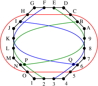
Figure 1: Critical KS sets 26-13 and 30-15. They, as well as other figures with odd number of edges below, vividly illustrate the parity proof: all vertices share two edges.

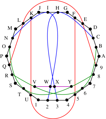
Figure 2: Critical KS sets 34-17 and 38-19. The latter one is drawn by Asymptote (vector graphic language). By changing parameters one can interactively control and change the shape of each edge line and unambiguously discern vertices that share an edge.

Parity Proof. By looking at the KS hypergraphs shown in Figs. 1 and 2, we see that we cannot ascribe values 0 and 1 to all vertices so that in each edge we ascribe 1 to one of the vertices and 0 to the others. Namely, in all these hypergraphs, each vertex shares exactly two edges, so there should be an even number of 1s. At the same time, each edge must contain one 1 by definition, and since there are an odd number of edges, there should be an odd number of 1s—a contradiction. This is the simplest form of the parity proofs of the Kochen-Specker theorem on KS sets.

In these parity proofs, as well as in more involved ones we give in [23], the essential part of the proof is that we have an odd number of edges. We found 90 kinds of such critical KS sets starting with a 26-13 and ending with a 60-41 one and presented them qualitatively in Table 3 of Ref. [23]. These KS set we found by means of the parity proofs in Ref. [23], but not by the algorithms we used for this paper, we indicated by “$\otimes$” in Table 1 below.

In Table 1 and Fig. 7, we show the distribution and numbers for each kind that were found by the random sampling of our present survey.

We prove the impossibility of assigning 0 and 1 to vertices by means our program states01, which exhaustively tests each hypergraph. For KS sets with an odd number of edges, we can also quickly verify their KS property with the help of the parity proof.

In the sample used for our survey, on average $3\cdot 10^{8}$ for each of 13–63 edges (1–12 and 64–75 were exhaustively scanned), we obtained 35 kinds of critical KS sets with an even number of edges, which cannot be obtained by the parity-proof method. We also obtained 62 kinds of critical KS sets with an odd number of edges. They are all among 90 kinds of KS critical sets we obtained by the parity-proof method in [23]. Those that we did not obtain in our samples are indicated by “$\otimes$” in Table 1. Our scanning in [23] was designed to obtain as many different kinds of critical sets as possible. So, we always stopped scanning as soon as we found a new kind and therefore we cannot estimate numbers of critical sets of each kind that would correspond to to numbers obtained in this paper and shown in Table 1.

	critical KS sets with odd number of edges															… with even number of edges
ver	13	15	17	19	21	23	25	27	29	31	33	35	37	39	41	24	26	28	30	32	34	36	38	40
26	1
30		3
32			1
33			2
34			5
36				11
37				9
38				6	10
39					30
40					38	10
41					22	5
42					6	16	3									1
43						22	38
44						14	16	$\otimes$
45						3	5	32									2
46						1	3	130	$\otimes$									3
47							1	74	$\otimes$									6
48							2	19	9	$\otimes$								11
49							$\otimes$	$\otimes$	11	1								3	9
50							1	$\otimes$	7	13									39
51								$\otimes$	1	33	$\otimes$								19	18
52								$\otimes$	$\otimes$	37	33								4	69
53								$\otimes$	$\otimes$	11	114	$\otimes$							1	73	45
54								$\otimes$	$\otimes$	$\otimes$	153	16								26	275
55									$\otimes$	1	56	158	$\otimes$							5	339	25
56									$\otimes$	$\otimes$	21	241	28								136	262
57										$\otimes$	1	133	378								54	448	45
58										$\otimes$	$\otimes$	30	678	27							2	256	493
59											$\otimes$	2	308	381							1	55	864	16
60											$\otimes$	$\otimes$	48	562	1							5	316	145

Table 1: List of KS critical sets we obtained in this paper. By $\otimes$ we indicate the existence of KS critical sets (at least one set) we obtained in [23] by the parity proof method. The average sample sizes of $3\cdot 10^{8}$ sets used here were too small to obtain them by our algorithms/programs.

In Figs. 3, 4, 5, and 6, we show some further examples of hypergraphs automatically drawn by our program written in Asymptote.

In the MMP notation for these (shown below), the numbers in parentheses [$(n)$] are the size of the maximal loops ($n$-gons) that the edges can form. The first $n$ edges (tetrads) form $n$-gons. We obtain them by our program loopbig. Additional examples of hypergraphs of each kind not given here are listed in A.

There are three types of edges in an MMP hypergraph

• those that form the $n$-gon.

• those that contain vertices that do not belong to the $n$-gon. We call that latter vertices free vertices.

• all others.

To better discern the vertices in an MMP hypergraph with over 24 vertices and over 40 edges, we usually represent them by two figures—one showing the $n$-gon with free edges and the other showing the $n$-gon with span edges.

42-24  (13)   3124,4VIU,UX97,7586,6WOd,dHBT,TRSM,MKJL,LcCb,bPGf,fgAe,eYQa,aZE3, 9ABC,DEF8,GHIJ,NOPQ,WXYF,ecVD,gUSO,ZTN7,bWR2,fK63,eJ72. Shown in Figs. 3..

50-30   (15)   3124,4DEF,Fm6i,ihbP,POQJ,JHIG,GoCj,jkKS,SRTU,UeLd,dl7W,WVNX,Xg8f,fnAZ, ZYa3,5678,9ABC,KLMN,bcaM,TQFC,ecEB,lkPA,mdZO,mgRI,iYKH,njcW,jhg4,VHA4,oaR7, oife.  Shown in Fig. 4.

54-34  (16)   1234,4567,789A,ABCD,DEFG,GHIJ,JKLM,MNOP,PQRS,STUV,VWXY,YZab,bcde, efgh,hijk,klm1,3EQb,5DWl,7JYk,8Ubl,CHXe,DKTa,EMfm,OTck,2nLZ,3To9,6FLq,7Nen,Bonm,IQWn,Ipdi,LRlp,Srsj,Ugrq.  Shown in Fig. 5.

60-40  (18)   3124,4576,6yau,uvVt,trqs,soTP,Pxh9,98AB,BpWM,MJLK,KicU,UwOl,lmnk,kjSH, HGIF,FCED,DYRf,feg3,,NOPM,QRSB,TUVW,XYZW,abcd,hiI2,odZS,pjc7,qLA6,wtbH,xvpg,yxnR, rhSJ,vOEA,mYP6,ieCB,oneG,ncXA,ulhf,reaO,wpoD,slB4  Shown in Fig. 6.

To obtain these hypergraphs, we used a procedure that strips one edge at a time. For $n$ input hypergraphs each with $b$ edges, $n\cdot b$ output hypergraphs, each with $n-1$ edges, were generated. After passing these output hypergraphs through several filters to eliminate unconnected hypergraphs, duplicates, non-KS (colorable) sets, and isomorphic sets, a smaller number of hypergraphs usually resulted. In order to keep the run time feasible, we took a semi-random sample of the generated hypergraphs so that in the end we would have approximately the same number $n$ of hypergraphs to send to the next edge-stripping step.

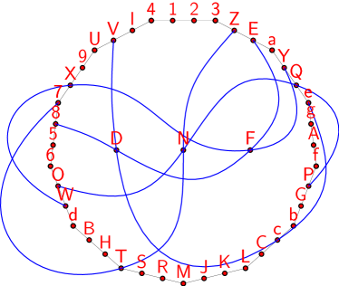
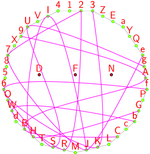
Figure 3: Critical KS sets with even number of edges. (a,b) presentations of 42-24 using the biggest loop (13-gon): (a) 13-gon with only free edges; (b) with only span edges; tension of the lines in (b) is higher for better discerning of the edges.

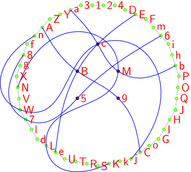
Figure 4: (a,b) 50-30 (15-gon): (c) free edges only; (d) span edges only. We can add or delete vertices and edges [as in of Fig. 3 and Fig. 6] according to an algorithm so as to obtain sub-hypergraphs for various applications, e.g, finding Hilbert space equations for quantum systems. [4, 5]

The programs we used and their algorithms are described in Sec. 3. We used the program mmpstrip to strip edges from starting hypergraphs. We adjusted the increment parameter of mmpstrip so that, after each edge removal and post-processing step, we ended up with a sample of a desired size, say 50,000 hypergraphs. We ended up with 64 sample sets of up to 50,000 hypergraph each, with one sample set for each hypergraph size from 12 through 75 edges. For 12 edges and less, no KS sets have ever remained, probably because they don’t exist.

The complete processing of the samples sets of this size, including finding all of the critical KS hypergraphs among them, took about 4 days on a single CPU. We ran 200 such jobs on a cluster, then combined the results. The random selection and the large sample space ensured that we would have, with high probability, completely different samples on successive program runs. Except near the extreme edge sizes of 75 and 12 where the sample space is essentially exhausted, we never found a duplicated hypergraph in our spot checking.

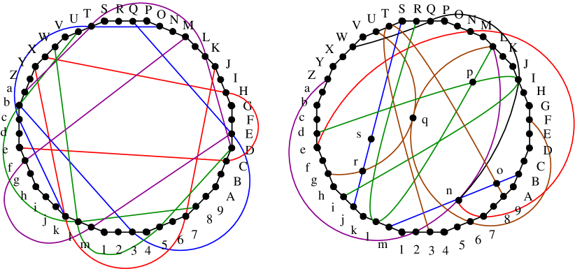
Figure 5: A critical 54-34 KS set shown in two figures. (a) A maximal 16-gon + span edges; (b) 16-gon + free edges.

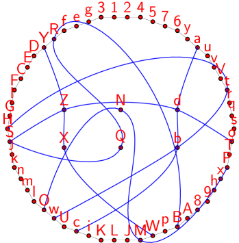
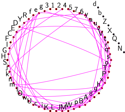
Figure 6: A critical 60-40 set; (a) A maximal 18-gon + free edges; (b) 18-gon + span edges. Letters and edges might appear overcrowded, but the MMP hypergraph offers a clear alternate representation for each of them. Also, by means of our programs, they can be easily discerned textually and visually. Actually, when an MMP figure of a KS set is shown as a figure, we need not give ASCII characters at all—we can always ascribe them to vertices in an arbitrarily chosen way later on.

The overall iterative procedure we used is as follows. We started with the MMP hypergraph for the 60-75 KS set.

1. We started with the 60-75 KS set and with mmpstrip obtained 75 new 60-74 sets—each with one less edge than the original 60-75. Then we repeated the procedure to obtain 2775 new 60-73 sets, etc. but not more than 50,000 hypergraphs (or a million for some studies) to keep the run time reasonable. We used mmpstrip’s increment parameter $i$, which selects every $i$th edge on average, to achieve this limit. The increment parameter can be a non-integer to better control the output size. When it is greater than 1, the edges can be selected either with uniform spacing or randomly; the latter option was usually chosen.

2. A hypergraph is connected if there is a chain of zero or more edges connecting every pair of edges. Unconnected hypergraphs were removed with mmpstrip.

3. Duplicate hypergraphs result when one edge is removed at a time (rather than multiple edges combinatorially). These duplicates were removed.

4. Isomorphic hypergraphs were removed with shortd.

5. Colorable hypergraphs were filtered out with states01, leaving only non-colorable ones (i.e. KS sets).

Typically, we first ran these steps on a small sample of the hypergraphs (a hundred or so) so that the increment parameter for each mmpstrip call could be estimated, in order to end up with the same number of output hypergraphs as input hypergraphs after each edge removal step.

We examined the final set of MMP hypergraphs obtained after each iteration of the above process in order to determine which hypergraphs were critical, using an option of the states01 program. Any critical sets found were collected for analysis.

The advantage of stripping one edge at a time then filtering at each stage is that many fewer MMP hypergraphs had to be examined, because at each step we consider only the non-isomorphic KS sets from the previous step. For example, from Fig. 7 (below), there are $3.1\cdot 10^{20}$ hypergraphs with 28 edges, of which only $1.6\cdot 10^{13}$ are KS sets. The 23 critical sets were were found by examining a sample of only $6\cdot 10^{7}$ KS sets rather than $1.2\cdot 10^{15}$ starting MMP hypergraphs that would have been required, representing a speedup factor of about 20 million.

3 Algorithms

For the purpose of the KS theorem, the vertices of an MMP hypergraph are interpreted as rays, i.e. 1-dim subspaces of a Hilbert space, each specified by a representative (non-zero) vector in the subspace. The vertices on a single edge are assumed to be mutually orthogonal rays or vectors. In order for an MMP hypergraph to correspond to a KS set, first there must exist an assignment of vectors to the vertices such that the orthogonality conditions specified by the edges are satisfied. Second, there must not exist an assignment (sometimes called a “coloring”) of 0/1 (non-dispersive or classical) probability states to the vertices such that each edge has exactly one vertex assigned to 1 and others assigned to 0.

For a given MMP hypergraph, we use two programs to confirm these two conditions. The first one, vectorfind, attempts to find an assignment of vectors to the vertices that meets the above requirement. This program is described in Ref. [18]. The second program, states01, determines whether or not a 0/1 coloring is possible that meets the above requirement. The algorithm used by states01 is described in Ref. [25]. An additional option was added to states01 to determine if a hypergraph is critical i.e. whether the hypergraph is non-colorable but becomes colorable if any single edge is removed.

The 60-vertex, 75-edge MMP hypergraph based on the 600-cell described above (which we refer to as 60-75) has been shown to be a KS set. [26] However, it has redundancies (is not a critical set) because we can remove edges from it and it will continue to be a KS set. The purpose of this study was to try to find subsets of the 60-75 hypergraph that are critical i.e. that are minimal in the sense that if any one edge is removed, the subset is no longer a KS set.

While the program vectorfind independently confirmed that 60-75 admits the necessary vector assignment, such an assignment remains valid when a edge is removed. Thus it is not necessary to run vectorfind on subsets of 60-75. However, a non-colorable (KS) set will eventually admit a coloring when enough edges are removed, and the program states01 is used to test for this condition.

A basic method in our study was to start with the 60-75 hypergraph and generate successive subsets, each with one or more edges stripped off of the previous subset, then keep the ones that continued to admit no coloring and discard the rest. Of these, ones isomorphic to others were also discarded.

The program mmpstrip was used to generate subsets with edges stripped off. The user provides the number of edges $k$ to strip from an input MMP hypergraph with $n$ edges, and the program will produce all $\binom{n}{k}$ subsets with a simple combinatorial algorithm that generates a sequence of subsets known as the “banker’s sequence.” [27] Partial output sets can be generated with start and end parameters. By default, mmpstrip will scan linearly through the edges to pick every $i$th one when the increment parameter is $i$. The program will optionally randomise this edge selection, so that while a fraction $1/i$ of edges is picked from each input hypergraph, which edges are picked are random. The goal of this feature is to lessen the chance of a biased selection due to a pattern that is repeated for every hypergraph (such as removing only the first edge from each hypergraph). It is hoped that the samples would thus provide a more uniform representation of the search space.

Optionally, mmpstrip can take truly random samples with replacement (for a given number of edges) from the starting 60-75 MMP hypergraph (in contrast to the semi-random method of the previous paragraph). This mode was used to verify or improve some of the statistical estimates in Fig. 7. A cryptographic hash of the time of day, process ID, and CPU time is used as the seed for the pseudo-random number generator. The seed may also be provided by the user in order to repeat a result.

The mmpstrip program will optionally suppress MMP hypergraphs that are not connected, such as those with isolated edges or two unconnected sections, since these are of no interest. The output lines are by default renormalized (assigned a canonical vertex naming), so that there are no gaps in the vertex naming as is required by some other MMP processing programs.

In order to detect isomorphic hypergraphs, one of two programs was used. For testing small sets of hypergraphs, we used the program subgraph described in Ref. [18], which has the advantage of displaying the isomorphism mapping for manual verification. For a large number of hypergraphs, we used Brendan McKay’s program shortd, which has a much faster run time.

Program longest singles out longest loops from the list of all possible loops (which is the output of the program loopbig). Programs parse or parse_all then “write” a program or programs in the vector graphics language Asymptote for drawing a chosen hypergraph or all hypergraphs, respectively.

The longest loop of each hypergraph is drawn as $n$–sided regular (equilateral and equiangular) polygon, where $n$ is the number of edges in the loop. By default, free vertices, i. e. vertices that are not on the loop, are placed inside the polygon, off–centre, on vertical lines, with not more than 4 vertices on one line, but the user can change options for their placement. Edges contained in the longest loop are drawn as straight lines, while other edges are drawn as Bézier curves (specifically, Asymptote is based on Donald Knuth’s METAFONT). The user can interactively change the “tension” of the curve and the amount of “curl” at its endpoints, in order to interactively control and change the shape of each edge line and unambiguously discern vertices that share an edge.

4 Sample Space Statistics

There are $3.8\cdot 10^{22}$ possible subsets of the 60-75 set (disregarding any symmetry) and, among them, approximately $7.5\cdot 10^{17}$ KS sets. An exhaustive search for critical KS sets was not feasible for the present survey, but it may become feasible in the future, possibly requiring a year or more on a large computer cluster.

For our survey, we searched a total of around $10^{10}$ KS sets, randomly chosen for a given edge size, to find the critical KS sets among them. We then performed a statistical analysis to estimate the total number of critical KS sets that would be found by an exhaustive search. The final result is that we can expect a total of $4.3\cdot 10^{12}$ non-isomorphic critical sets, with a 95% confidence interval between $4.0\cdot 10^{12}$ and $4.6\cdot 10^{12}$ based on the statistical model we used.

If an exhaustive search is performed, it is possible to store the complete set of non-isomorphic critical sets with current technology. Without compression, each critical set (in MMP hypergraph notation) requires an average of about 260 bytes, thus requiring $260\cdot 4.3\cdot 10^{12}=1.1\cdot 10^{15}$ bytes (1.1 petabytes) of storage. This could probably be reduced considerably with data compression techniques.

The plots of Fig. 7 provide an overview of the subsets of 60-75, broken down by the number of edges. These plots are intended to provide a guideline for estimating the work that would be required for an exhaustive search for a particular number of edges or range of them.

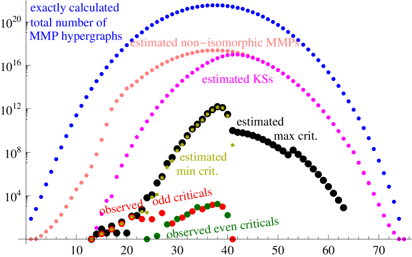
Figure 7: Overall statistics calculated for subsets of 60-75 given on a logarithmic scale. The samples (for 13-63 edges; 64-75 search was exhaustive) contained on average $3\cdot 10^{8}$ MMP hypergraphs. “Observed odd (even) criticals” refer to odd (even) numbers of critical KS sets. The sudden jump in the “estimated max crit.” plot at 53 edges is caused by a change in the sample size, as explained in the text. The “estimated min crit.” points are not plotted when they are zero. The “estimated max crit.” for more than 63 edges are not shown since the exhaustive search found no criticals there.

The details of the statistical methods we used, as well as a more detailed description of Fig. 7, are given in B.

In our survey, no critical sets were observed in KS sets with 42 or more edges. In these cases, the “estimated max crit.” in Fig. 7 has little to do with the number of critical sets (if any) that actually exist in that edge range. Instead, it could be interpreted as “zero with statistical noise” and is primarily a function of the number of samples we took and the search space size for the particular edge size. It simply indicates that, based on a Bernoulli trial probability model, it is unlikely (with 95% confidence) that there are more critical sets than “estimated max crit.” The sudden jump between 52 and 53 edges is due to the fact that we changed the number of samples from $5.3\cdot 10^{7}$ per edge size to $8.6\cdot 10^{6}$. If an exhaustive search shows that there are no critical sets at all above 41 edges, that will be completely consistent with the “estimated max crit.” bound. In fact, we would conjecture that the actual number of critical sets will be identically zero very soon after 41 edges (see the last paragraph of B).

5 Conclusions

Kochen-Specker (KS) sets and setups proposed, designed, and experimentally carried out so far were either 3-, 4-, 8-, …dimensional KS sets (Peres’, Cabello’s, etc.) or the Mermin set. They aim at finding particular valuation of the KS observables that prove the quantum contextuality and disprove any noncontextual classical valuations of those observables. Our aim is to make KS sets independent of a particular choice of either vectors or observables so as to make them suitable for building quantum gates within a would-be quantum circuit.

For this application, we should have a choice of gates of different sizes, that is, consisting of sufficiently many vectors and sufficiently many gates for a chosen number of vectors, and this is what we achieved in the previous sections. We generated a large number of 4-dim critical non-redundant non-isomorphic KS sets with 26 to 60 vectors based on the 600-cell (the 4-dimensional analog of the icosahedron). “Critical” means that no orthogonal tetrads can be removed without causing the KS contradiction to disappear. In other words, they represent a KS setup that has no experimental redundancy.

The generation was achieved by algorithms and computer programs described in Sec. 3, with which we found the critical sets summarized in Fig. 7. Previously, only two 30-15 critical KS sets were found by Waegell and Aravind [28] as well as a new third class. In this work, we have extended our previous study of up to 19 edges [22] to sample the entire range of all 60-75 subsets. The number of critical sets with the lowest number of edges, 13 through 19, appears comparatively small, and it is feasible to find all of them with an exhaustive search. Beyond that, the number of non-isomorphic classes becomes very large and attempting their generation now would take too many CPU months on the grid. In Sec. 4 and B, we give the detailed statistical estimates of the total critical sets that exist based on our samples. The statistical techniques we used are general-purpose and can be useful for any similar experiment in which an exhaustive enumeration of outcomes is not feasible.

We stress here that critical sets obtained by a future exhaustive generation might well be far less numerous then their statistical estimates given above. That would be yet another proof of how different quantum sets are from classical ones and how cautious we should be when interpreting classical statistical methods applied to quantum data. This is also the reason why we have not and could not have made any realistic predictions on numerosity and existence of critical sets that might be observed in the future but have not been observed so far. All we can say right now is that the predicability of the total number of KS sets is in good agreement with the data we so far obtained by exhaustive generation. For example, by exhaustive generation of KS sets with 63, 64, 65, and 66 edges we obtain $1.8\cdot 10^{9}$, $4.1\cdot 10^{8}$, $1.0\cdot 10^{8}$, and $1.1\cdot 10^{7}$ sets versus estimated $1.8\cdot 10^{9}$, $3.4\cdot 10^{8}$, $5.7\cdot 10^{7}$, and $8.8\cdot 10^{6}$, respectively.

The main theoretical results of our generation are that

• the 24-24 and the 60-75 classes are disjoint (in the sense that the biggest set of the 24-24 class is the single Peres’ 24-24 set and the smallest set from the 60-75 class is the 26-13 one;

• the maximal loop of all sets from the 24-24 class is always a hexagon while the maximal loops of the sets from the 60-75 class grow (form at least an octagon) as the number of vectors and edges increase (see Figs. 1-6);

• there is an unexpectedly large and rich universe with an estimated $4.3\cdot 10^{12}$ non-isomorphic critical sets inside of the 60-75;

• in [4] we found that one of the known 3-dim KS sets passes a series of equations that hold in any Hilbert space—the so-called orthoarguesian equations. We have not found any such KS set in the 60-75 class so far. Both results show that orthogonality of vectors does not suffice for a complete Hilbert space description of KS sets—the relations between nonorthogonal vectors play an essential in such a description. This will prove essential for a proper description of quantum gates using KS sets;

• there is only one KS set with 24 vectors (vertices) and 24 tetrads (edges), and it contains all KS sets from the 24-24 class with the chosen values of vector components. [18] In contrast to this, there are many non-isomorphic KS sets with 60 vectors and 60 tetrads which contain many non-isomorphic KS subsets each.

Another open question is to find physical and geometrical reasons for having only hexagon maximal loops in the 24-24 class and for having particular octagons, nonagons, decagons, etc., in the 60-75 class.

Appendix A Samples of KS hypergraphs with even number of edges

Here we give samples of KS hypergraphs of each kind that we listed in Table 1 and did not give in Figs. 1–6 and in Sec. 2.

Using our programs longest and loopbig, we can instantly determine the following structural features. Let us take the 45-26 hypergraph below. The program longest shows that its biggest loop is a 12-gon. The program loopbig gives 26 instances of its 12-gon representation, the first one of which is 2134,4YZE,EFGD,DfKN,NPQO,OeUd,dacb,bWL7,7586,6jMT,ThgV,ViR2. 9.A.B.C. H.I.G*8* J.K*L*M*R*S.Q*C. T*U*S.F* V*W*X.P* c*X.M*3* f*Z*R*7* g*e*I.3* i*j*Y*N* h*a*Y*H. a*B.6*2* e*Y*L*A. d*V*K*9. (The edges are the same as in 45-26 below, only in a different order. Also the vertices within an edge are mostly in a different order. Actually, all 26 instances are just different 12-gon arrangements of 45-26 below.) The edges 1234–ViR2 are polygon edges (see Sec. 2); vertices followed by “.” are free vertices; edges containing free vertices are free edges; vertices followed by “*” are polygon vertices; edges containing only polygon vertices followed by “*”s are span edges; (in other words span edges are edges which are not polygon edges and which do not contain free vertices). Our script based on Asymptote draws 26 figures of 45-26 with 12-gons. Once the figures are drawn, the user can assign any ASCII symbol desired to any vertex. Also, by utilizing our program vectorfind she/he can ascribe vectors to vertices. 1,2,…,i,j $\to$ {$\tau$,0,$\overline{1}$,$\overline{\kappa}$}, {0,1,0,0}, {$\kappa$,0,$\tau$,$\overline{1}$}, {1,0,$\kappa$,$\tau$}, {$\kappa$,$\tau$,1,0},  {$\overline{1}$,0,$\kappa$,$\tau$}, {$\overline{\tau}$,$\kappa$,0,$\overline{1}$},  {0,$\overline{1}$,$\tau$,$\overline{\kappa}$}, {0,$\tau$,$\kappa$,1},  {1,$\overline{1}$,1,1}, {$\overline{\kappa}$,0,$\tau$,$\overline{1}$},  {$\tau$,$\kappa$,0,$\overline{1}$}, {$\overline{1}$,1,1,$\overline{1}$},{$\overline{1}$,1,$\overline{1}$,1}, {$\overline{1}$,$\overline{1}$,1,1},  {1,1,1,1}, {$\overline{\kappa}$,$\overline{1}$,0,$\tau$},  {$\tau$,$\overline{1}$,$\overline{\kappa}$,0},  {$\kappa$,$\overline{\tau}$,$\overline{1}$,0},  {0,$\overline{1}$,$\tau$,$\kappa$},  {$\overline{1}$,0,$\overline{\kappa}$,$\tau$},{$\tau$,$\kappa$,0,1},  {$\tau$,1,$\kappa$,0}, {$\kappa$,0,$\overline{\tau}$,$\overline{1}$},  {0,$\kappa$,$\overline{1}$,$\tau$},  {$\overline{1}$,$\tau$,0,$\overline{\kappa}$},  {0,0,1,0}, {$\kappa$,1,0,$\tau$}, {0,$\overline{1}$,$\overline{\tau}$,$\kappa$},  {$\tau$,$\overline{1}$,$\kappa$,0}, {1,0,0,0}, {0,1,$\tau$,$\kappa$},  {0,$\tau$,$\overline{\kappa}$,$\overline{1}$}, {$\overline{1}$,$\kappa$,$\tau$,0},  {$\overline{1}$,$\overline{\tau}$,0,$\kappa$}, {$\tau$,0,1,$\kappa$},  {$\kappa$,$\tau$,$\overline{1}$,0}, {$\overline{1}$,1,1,1},  {0,$\overline{\kappa}$,$\overline{1}$,$\tau$}, {1,$\tau$,0,$\kappa$},  {$\kappa$,$\overline{1}$,0,$\overline{\tau}$},  {0,$\kappa$,$\overline{1}$,$\overline{\tau}$}, {0,$\overline{\tau}$,$\kappa$,$\overline{1}$}, {0,0,0,1}, {$\overline{\kappa}$,$\tau$,$\overline{1}$,0}, where $\tau=(\sqrt{5}+1)/2$ and $\kappa=1/\tau$; a bar over a number indicates its negative.

45-26   1234,5678,9ABC,DEFG,HIG8,JKLM,NOPQ,RSQC,TUSF,VWXP,YZE4,abcd,edUO,cXM3,fZR7,bWL7,geI3,fNKD,hgVT,ijYN,haYH,jTM6,aB62,iVR2,eYLA,dVK9.

46-28   1234,5678,9AB8,CDEF,GHIJ,KLMN,OPQR,STR4,UVNF,WXYZ,abZT,YQME,cdYB,efb7,gVSJ,hiPA,jfOI,idHD,aLIC,ieXN,jiS6,kgM5,khcG,kbU9,hL73,cON2,WSL9,gZOD.

47-28   1234,5674,89AB,CDEF,GHIJ,KLJ7,MNOB,PQR3,STUO,VWU6,XYI5,ZabL,cdYL,efbF, gaHA,hWG9,iTGE,jkZ2,lkNE,kdUR,lfXK,hXD1,XVQ8,jfPA,jcMC,ecSQ,khge,iaXM.

48-28   1234,5678,9ABC,DEC8,FGHI,JKLM,NOME,PQRB,STIA,UVWX,YXRL,Zab4,cdW3,efgT, hdbK,ijcJ,gVQH,kfJG,lhF7,jeb6,iUPD,faU9,YS72,mlZT,lQO3,kdYN,mUN6,iZYH.

49-28   1234,5678,9ABC,DEFG,HIJ8,KLG7,MNOP,QRSP,TUVJ,WLC4,XYZV,abS7,cdeb,fgUO, heZN,ijdI,kgaF,lcYM,jYRE,iXQG,fHGB,mfdW,mkTN,nhR3,nigA,lhFC,cTG3,mYA7.

49-30   1234,5678,9ABC,DEFG,HIJK,LMN8,OPQR,STUK,VWRC,XYZW,abcQ,deJ4,fghe,ijU3, kjQG,ZTNB,khA7,gYS8,lkV2,mcMF,mif6,lidE,nfXD,mPJB,gOI3,bX73,ndcC,lgaB,nkNI,lXMK.

51-30   1234,5678,9AB8,CDEF,GHIJ,KLMN,ONJ4,PQRS,TUB3,VWIA,XSOF,YZE7,aHD6,bcZX, defW,ghiM,cWR2,jkL9,liR5,mbUC,nkfb,onha,pgeX,pojG,mhdQ,oYP3,pmVK,nlTK,kgYH,ljd4.

52-30 1234,5678,9ABC,DEF4,GHIJ,KLMN,OPQ8,RSQJ,TUVI,WXYZ,abcJ,NHC3,defg,hijc,kgbB,lkZ7,mYMJ,njX4,fSNF,oWVA,piPA,qeVE,onml,qpna,ohdQ,pfYU,liLE,UQLB,qhN7,ngI8.

53-30   1234,5678,9ABC,DEFG,HIJK,LMNO,PQRS,TUVW,XYZW,abZS,cdVG,eRC4,fghY,ihK3, gdbJ,jkeI,lQOF,mki8,nopJ,qpjE,qhP7,roX7,nmUQ,rjcN,rfUB,pliT,paMB,mYNC,MIG7,lbC7.

51-32 1234,5678,9AB4,CDEF,GHFB,IJKL,MNOP,QRPL,STUH,VWXR,YZUQ,abcO,dZXE,eTK8,fgJA,hig3,jiN7,iSD9,khcY,lXMK,mnWA,opYI,ndc6,ljfC,mjZ2,lbS5,pV62,piaG,ogeb,keWG,onPC,kSP2.

52-32 1234,5674,89AB,CDE7,FGHB,IJKL,MLA3,NOP2,QRST,UVWX,YZaX,bcWT,dePK,fgSJ,hiaH,jkOG,lmW9,nmgN,oeVR,kife,pkZQ,pcE3,onHE,qjRM,qfbY,hbND,qp96,laR4,UJGD,qndU,dZB7,RNIB.

53-32 1234,5678,9A84,BCDE,FGHI,JKLM,NOPQ,RST3,UVW7,XYIA,Zabc,defM,ghYL,ijcT,kWQ2,ljfH,mhbV,nmiP,eSGE,oaUK,pgZR,qohO,plNK,ondI,ZXE2,rfUD,gdC6,qiD9,rpmk,qkJG,cNG5,mHC3.

54-32 1234,5678,9ABC,DEFG,HIJC,KLMN,OPQR,STUC,VWXY,URN4,Zabc,def3,ghcQ,ihMJ,jkB8,lifY,mkgT,nopA,qrlT,rpjP,ebX8,rhdG,qoeJ,maPF,naNI,sbLE,som7,oZYG,nWTE,rVN7,fQEB,YPLC.

55-32 1234,5678,9ABC,DEFC,GHIJ,KLMF,NOPQ,RSTU,VWXY,ZabE,cde8,fghe,ijeQ,klmU,mhbJ,nopB,qrpT,sjT4,todY,naMI,SHA3,tlP7,ngR7,rGF7,qZXO,tsZL,eWM3,fVLA,nmiV,dNF4,qkdA,mOC8.

53-34     1234,5674,89AB,CDEF,GHIJ,KLMN,OPQR,STUV,WVRB,XYUF,Zabc,decN,fgYJ,hijA, kjbE,lmQF,ePI3,aWMI,niXL,oZRH,phcT,pmH7,qkLB,pgKE,qhI6,rnmf,ncO2,mdSA,OJDA,roke,ogS6,lLJ4,raU4,nIE9.

55-34       1234,5674,89AB,CDEF,GHIJ,KLJ7,MNOP,QRST,UVWT,XYZa,bcaW,dec6,fghI,ihPB, jkgS,kZVL,lmRO,noi3,pqYI,rNF3,qoeE,mbDA,sljc,rplU,sfXQ,kbH2,tsqN,ndYO,tU97,nfLA,reSJ,XUPH,siJD,kOE9.

56-34   1234,5674,89AB,CDEF,GHIJ,KLMN,OPQR,STUJ,VWXB,YURN,Zabc,defT,ghMF,ijQE, klmA,nLI9,opnc,pmhY,qjbH,oKD8,olX7,rsfa,iWS3,tsWM,utZP,urmJ,neO6,uqog,dHF3,skH6,qYV4,laIE,ieZY,fPD4.

57-34     1234,5674,89AB,CDEF,GHIJ,KLMN,OPQB,RSTU,VWXY,Zabc,defc,ghb7,ijkY,lmnU, ofT3,pqSA,rstR,qnXQ,uvmN,pkhN,ljgP,ieMA,tolJ,vdWI,aQJF,ueVP,ZPLE,sPI4,RNHD,voiZ,rnL3,bYDB,rpVF,dRQ7.

58-34   1234,5678,9ABC,DEF8,GHIJ,KLMN,OPQN,RSTU,VWXY,ZaMJ,bYU4,cdef,ghia,jkiQ, lmnT,onP8,phfL,qoeS,rROI,hbHC,srp3,qpmX,tuvo,wvdJ,wqb7,rkdK,jcWB,uscb,trlB,ukVT,lbZF,gVIF,vpjF,qgNB.

59-34     1234,5678,9ABC,DEFG,HIJK,LMNO,PQR8,STUV,WXYZ,abcZ,defg,higO,jklm,nopm, qric,slbR,tukQ,uV74,vuYN,srf3,paN3,wthC,jeKB,xwvj,qodX,xqUQ,jVMG,UJF3,nIC8,wWTH,cTE8,snWM,wdRF,oTOB.

55-36   1234,5678,9AB4,CDEF,GHIJ,KLMF,NOP3,QRPM,STUJ,VWOB,XYZa,bcdA,efgh,ijkd, lmkU,haNJ,nocW,pREB,qrpj,mbZ2,ojJD,srM8,qgb7,tlaW,WTF7,qnQI,kYHE,sZIB,fXOD,iL62,tfI6,qSOL,leLA,neE8,rWH2,kfM4.

56-36   1234,5674,89AB,CDEF,GHIJ,KLMF,NOPQ,RST3,UVWX,YZaX,bcdW,efgB,hVE7,ijgQ, kTPM,lmnd,oQJD,pqrs,faC2,tsnI,kjcA,tZOA,uib6,mYS9,uonf,rliR,sUQL,qXPH,poZ4,rG97,mkeU,hRIB,qmh2,mOK6,ocRK,bPC9.

57-36     1234,5674,89A3,BCDE,FGHI,JKLM,NOPQ,RSTU,VWXY,ZaYQ,bcdI,efE2,ghM3,ijkf, lhda,mecP,nOL7,oXU6,pqbA,kNHD,rsqZ,pnfT,cWSK,ZJGE,tunl,vsVO,ljUG,vgTD,umiR,oiOI,rmh6,iWCA,vtA6,usH4,mYD9,qlKD.

58-36   1234,5674,89AB,CDEF,GHI3,JKLM,NOPQ,RSTM,UVB7,WXYI,ZaYT,bcaQ,dcSF,efgh, ijkR,lmhP,ngXL,nmZH,opWV,qplK,rpaA,sJE4,trkG,tnD9,usoZ,vfbI,qjf6,wXO6,wtse,vtld,kbVC,uhUM,wpiF,ujdN,kh84,pnN4.

59-36     1234,5674,89AB,CDEF,GHB7,IJKL,MNOP,QRPF,STUV,WXYA,ZabL,cdef,ghij,kfbY, kVR6,lKH3,mjO9,nopX,qrlU,siXT,tule,vwpS,odRK,xusJ,xwc6,thYG,daOE,wrm2,iND4,uZSA,xqF9,rnfN,vtNL,rgEA,phPJ,XLF2.

60-36   1234,5678,9AB8,CDEF,GHIJ,KLMN,OPQJ,RSTU,VWXN,YZab,cdeB,fgX7,hgeM,ijQF, kljd,mnoN,phbI,qrif,saEB,tolH,uvn4,srUL,wMD3,xmkf,wroZ,vcbT,ywjS,hWSP,ukYL,kVTJ,yvHE,uqP8,xUH8,tfbD,poQB,fSB4.

57-38   1234,5674,89AB,CDE7,FGHI,JKLM,NOPB,QRS3,TUVW,XYZa,bcde,fgPM,heWE,ijVS, klRI,mnol,podH,qrU6,sraP,toOL,ukaK,tgZG,cKD3,vspQ,vueO,vTJ7,vqgA,pkjh,nibP,jfcY,rmjG,nY94,viXI,tiE2,tkT9,qYHE,mQEB,cUIB.

58-38     1234,5674,89AB,CDEB,FGHI,JKL7,MNOP,QRST,UVWX,YZaA,bcLE,defg,hia3,jkXP, lmZK,ngWT,opnI,qrkH,rpSB,sfRO,tjRK,sYVL,umUG,vcPF,wm96,qeUD,okid,udbQ,wdYN,vpf2,wnhc,qnMK,utra,viW9,sliD,wtD2,QPD7,usn4.

59-38   1234,5674,89A3,BCD7,EFGH,IJKL,MNOL,PQRS,TUVW,XYZW,abZ2,cdeb,fgK6,hijA, aVSH,klJ9,mnoG,pID8,qrYC,stO1,oeRO,ujgF,vuol,wutU,xkid,wnZJ,mjcX,rfdQ,rhaN,xwPC,vcNE,qpkR,wpfM,vpV5,rmT8,tmkB,sWPF,vsiK.

60-38     1234,5674,89A7,BCDE,FGHI,JKLM,NOPE,QRST,UVWT,XYZa,bcde,fghA,eWMI,ijkl, mnlV,opha,qrgU,spnD,tdL3,trSP,cZRK,uveO,qkYI,jRHD,wrZ9,xiQ4,vtXV,mJC7,ywN6,yxtf,pibN,ysKG,wjhd,romG,upT2,xumY,yqC2,viGA.

59-40   1234,5678,9ABC,DEF8,GHI4,JKLM,NOPI,QRSC,TUVW,XYZH,abMB,cWPC,debZ,fgh7, ijkF,lmnk,opje,qnaV,rsmU,tjU3,lhYS,uSE2,sqdA,kgXR,upfO,vTQN,qfL3,wnNK,vuJG,wfbF,xicK,tgcE,vqoX,xura,xlTA,vcb6,spcY,rgeN,leG8,XUK8.

Appendix B Details for Sample Space Statistics

The plots of Fig. 7 provide an overview of the subsets of 60-75. Because they were determined by statistical inference from small samples of this space, most of the numbers are approximate. As a practical matter, some of the sample sets, or portions of them, were obtained with the more efficient semi-random method mentioned in the first footnote in Section 2, which has an effect. Overall, the numbers should be trusted only to within an order of magnitude or so. The plots are intended to provide a rough guideline for planning future work, such as an exhaustive search of certain ranges, and for that purpose it should be adequate.

Several techniques, which we describe below, were used to obtain the values for the plots. The total number of MMP hypergraphs is simply $\binom{75}{b}=\frac{75!}{b!(75-b)!}$, where $b$ is the number of edges given at the abscissa.

The mmpstrip program was used to identify and remove unconnected hypergraphs. We do not include the resulting numbers of MMP hypergraphs in Fig. fig:stat but briefly describe them as follows. For 1 through 4 edges, the number of unconnected MMP hypergraphs are exactly 0, 2175, 59725, and 1101450. For 67–75 edges there are exactly 0. For the rest, we used samples of $10^{6}$ MMP hypergraphs for each number of edges. For 47–66 edges, no unconnected hypergraphs were observed. For 5–46 edges, the number of unconnected hypergraphs (estimated from the ones observed in the sample) decreases to zero as a percentage the total number of MMP hypergraphs, from $1.56\cdot 10^{7}$ (out of $1.73\cdot 10^{7}$ total) for 5 edges to $1\cdot 10^{15}$ (out of $5.1\cdot 10^{20}$ total) for 46 edges.

To calculate the the number of non-isomorphic MMP hypergraphs, unconnected hypergraphs were discarded and the rest passed through the shortd program, which filters isomorphic hypergraphs, keeping only one canonical representative from each isomorphism class. For small and large numbers of edges, exhaustive generation of all MMPs yielded exact values. For 1–4 edges there are 1, 1, 2, and 5 (connected) isomorphism classes; for 67–75 edges, there are 1183189, 141314, 15014, 1463, 154, 19, 4, 1, and 1. For the other edge sizes, the number of isomorphism classes was estimated from a sample. Finding this estimate is called the “coupon collector’s problem,” [29] and the maximum likelihood estimator is the smallest integer $j\geq c$ such that

$$\frac{j+1}{j+1-c}\left(\frac{j}{j+1}\right)^{n}<1,$$ (1)

where $n$ is the number of samples (with replacement) and $c$ is the observed number of isomorphism classes in the sample. For example, we observed $c=516604$ isomorphism classes in a random sample of $n=545961$ 13-edge hypergraphs. The criteria of Eq. (1) yields $j=4893025\approx 4.9\cdot 10^{6}$, which is the point shown for 13 edges in the non-isomorphic MMP hypergraphs plot of Fig. 7. We mention that in our implementation, we expressed Eq. (1) as $\log(j+1)-\log(j+1-c)+n(\log j-\log(j+1))<0$ and determined $j$ with a binary search method. Because the computation involves the subtraction of almost-equal terms, high-precision floating-point operations are necessary. For the calculations of Fig. 7, Eq. (1) gave incorrect answers with less than 35 significant digits, and we used 100 significant digits for robustness.

As a rough check of the statistical model used by the coupon collector’s problem, 10 random samples of 50000 67-edge MMP hypergraphs yielded from 48900 to 48975 isomorphism classes, corresponding to predictions of 1119613 to 1202764 total classes by Eq. (1). This compares to the actual number of 1183189 classes obtained by exhaustive generation of MMP hypergraphs.

To estimate the KSs in Fig. 7, KS sets were identified using the states01 program. For small numbers of edges ($\leq 12$), we never observed a KS set. For large numbers of edges ($\geq 63$), we never observed a non-KS set, so for them the two plots coincide. For those in between, we took a random sample of non-isomorphic hypergraphs for each edge size and plotted the fraction of observed KS sets times the estimated non-isomorphic MMP hypergraphs.

We show the number of isomorphically unique critical hypergraphs we observed, as identified by the -c (“critical”) option of the states01 program, in the “observed odd criticals” and “observed even critical” plots of Fig. 7. We include these to show the actual currently known (not estimated) number of critical sets. It is not, however, intended to convey the distribution of critical hypergraphs vs. edge size; for that purpose, the estimated maximum number of critical sets in Fig. 7 should be used.

In the range of 12 through 62 edges, the “estimated max crit.” plot shows the upper 95% confidence limit derived from Bernoulli trial probabilities, based on the model of sampling with replacement from a search space where the a priori probability is unknown. [30] If $K$ is the total number of KSs (from the “estimated KSs” plot), $n$ is the sample size (with replacement) of random KS sets, and $m$ is the observed number of critical sets, then the lower 95% confidence level is [30, Eq. (1)]

$$K\cdot I^{-1}_{\frac{1}{2}(1-0.95)}(m+1,n-m+1)$$ (2)

and the upper 95% confidence level is [30, Eq. (3)]

$$K\cdot I^{-1}_{\frac{1}{2}(1+0.95)}(m+1,n-m+1)$$ (3)

where $I^{-1}$ is the inverse regularized incomplete beta function. For example, for the 35-edge case, $K=9.0\cdot 10^{15}$, $n=52800000$, and $m=580$. Thus for upper 95% confidence level we have $K\cdot I^{-1}_{\frac{1}{2}(1+0.95)}(m+1,n-m+1)=K\cdot I^{-1}_{0.975}(581,52799421)\approx K\cdot 0.0000119163\approx 1.1\cdot 10^{11}$. This is the value in the “estimated max crit.” plot for 35 edges.

The “estimated min crit.” plot shows either the the lower 95% confidence limit from Eq. (2) or zero (in which case we omit the “estimated min crit.” point from the plot since it is outside the logarithmic scale). A value of zero is used whenever no critical sets were observed. Of course this is the most conservative value possible, but there are two other motivations. First, the trend of the “estimated max crit.” curve starts to fall rapidly at 41 edges, and a smooth extrapolation would suggest that it plummets, perhaps to zero, very soon after that point. Second, when no critical sets were observed for a given edge size, the probability distribution of the Bernoulli trial estimation is not “Gaussian-like” but is highly skewed, with a mode (maximum likelihood) of zero critical sets, even though Eq. (2) may predict a small positive number.

We emphasize that in the cases where no critical sets were observed, “estimated max crit.” merely represents a statistical upper bound based on the number of random samples we took, meaning it is improbable that the actual number of critical sets would exceed that number. For sizes greater than 41 edges where no critical sets have been observed, there may be an overriding theoretical reason (that is currently unknown) that would lead to the actual number of critical sets being zero. In that case, “estimated max crit.” would get smaller and smaller, approaching zero, as we increased the number of samples. But for any given number of samples, the statistical upper bound is the best we can do without either a proof that the number of critical sets is zero or an exhaustive set of samples (which would amount to that proof). Thus the estimated range on Fig. 7 is as objectively conservative as possible, even though there is subjective evidence, based on extrapolation at 41 edges, that the actual number of critical sets becomes identically zero very soon after that point.

Acknowledgements  One of us (M. P.) would like to thank his host Hossein Sadeghpour for a support during his stay at ITAMP. Supported by the US National Science Foundation through a grant for the Institute for Theoretical Atomic, Molecular, and Optical Physics (ITAMP) at Harvard University and Smithsonian Astrophysical Observatory and by the Ministry of Science, Education, and Sport of Croatia through Distributed Processing and Scientific Data Visualization program and Quantum Computation: Parallelism and Visualization project (082-0982562-3160). Computational support was provided by the cluster Isabella of the University Computing Centre of the University of Zagreb and by the Croatian National Grid Infrastructure.

References

- [1] M.Hein, J. Eisert, H. J. Briegel, Multiparty entanglement in graph states, Phys. Rev. A 69 (2004) 062311–1–20.
- [2] A. Cabello, P. Moreno, All-versus-nothing proofs with n qubits distributed between m parties, Phys. Rev. A 81 (2010) 042110, ArXiv:1004.4874v1.
- [3] A. Cabello, Proposal for revealing quantum nonlocality via local contextuality, Phys. Rev. Lett. 104 (2010) 2210401–1–4, ArXiv:0910.5507v4.
- [4] M. Pavičić, B. D. McKay, N. D. Megill, K. Fresl, Graph approach to quantum systems, J. Math. Phys. 51 (2010) 102103–1–31.
- [5] N. D. Megill, M. Pavičić, Kochen-Specker sets and generalized Orthoarguesian equations, Ann. Henri Poincaré 11, ArXiv:abs/1005.0016.
- [6] M. Pavičić, Exhaustive generation of orthomodular lattices with exactly one non-quantum state, Rep. Math. Phys. 64 (2009) 417–428.
- [7] C. Simon, H. Weinfurter, M. Żukowski, A. Zeilinger, Feasible Kochen–Specker experiment with single particles, Phys. Rev. Lett. 85 (2000) 1783–1786.
- [8] M. Michler, H. Weinfurter, M. Żukowski, Experiments towards falsification of noncontextual hidden variables, Phys. Rev. Lett. 84 (2000) 5457–5461, ArXiv:quant-ph/0009061.
- [9] A. Cabello, “All versus nothing” inseparability for two observers, Phys. Rev. Lett 75 (2001) 010403–1–4, ArXiv:quant-ph/0101108v5.
- [10] Y.-F. Huang, C.-F. Li, J.-W. P. Yong-Sheng Zhang, G.-C. Guo, Experimental test of the Kochen–Specker theorem with single photons, Phys. Rev. Lett. 90 (2003) 250401–1–4.
- [11] Y. Hasegawa, R. Loidl, G. Badurek, M. Baron, H. Rauch, Quantum contextuality in a single-neutron optical experiment, Phys. Rev. Lett. 97 (2006) 230401–1–4.
- [12] A. Cabello, S. Filipp, H. Rauch, Y. Hasegawa, Proposed experiment for testing quantum contextuality with neutrons, Phys. Rev. Lett. 100 (2008) 130404–1–4.
- [13] H. Bartosik, J. Klep, C. Schmitzer, S. Sponar, A. Cabello, H. Rauch, Y. Hasegawa, Experimental test of quantum contextuality in neutron interferometry, Phys. Rev. Lett. 103 (2009) 040403–1–4.
- [14] G. Kirchmair, F. Zähringer, R. Gerritsma, M. Kleinmann, O. Gühne, A. Cabello, R. Blatt, C. F. Roos, State-independent experimental test of quantum contextuality, Nature 460 (2009) 494–497, ArXiv:0904.1655v2.
- [15] E. Amselem, M. Rådmark, M. Bourennane, A. Cabello, State-independent quantum contextuality with single photons, Phys. Rev. Lett. 103 (2009) 160405–1–4, ArXiv:0907.4494v2.
- [16] B. H. Liu, Y. F. Huang, Y. X. Gong, F. W. Sun, Y. S. Zhang, C. F. Li, G. C. Guo, Experimental demonstration of quantum contextuality with nonentangled photons, Phys. Rev. A 80 (2009) 044101–1–4.
- [17] O. Moussa, C. A. Ryan, D. G. Cory, R. Laflamme, Testing contextuality on quantum ensembles with one clean qubit, Phys. Rev. Lett. 104 (2010) 160501–1–4, ArXiv:0912.0485.
- [18] M. Pavičić, N. D. Megill, J.-P. Merlet, New Kochen-Specker sets in four dimensions, Phys. Lett. A 374 (2010) 2122–2128.
- [19] A. Peres, Two simple proofs of the Bell–Kochen–Specker theorem, J. Phys. A 24 (1991) L175–L178.
- [20] M. Pavičić, J.-P. Merlet, B. D. McKay, N. D. Megill, Kochen–Specker vectors, J. Phys. A 38 (2005) 1577–1592, and 38, 3709 (2005) (corrigendum).
- [21] A. R. Swift, R. Wright, Generalized Stern-Gerlach experiments and the observability of arbitrary spin operators, J. Math. Phys. 21 (1980) 77–82.
- [22] M. Pavičić, N. D. Megill, P. K. Aravind, M. Waegell, New class of 4-dim Kochen-Specker sets, J. Math. Phys. 52 (No. 2).
- [23] M. Waegell, P. K. Aravind, N. D. Megill, M. Pavičić, Parity proofs of the Bell-Kochen-Specker theorem based on the 600-cell, Found. Phys. 41 (2010) 883–904.
- [24] M. Waegell, P. K. Aravind, Critical noncolorings of the 600-cell proving the Bell-Kochen-Specker theorem, J. Phys. A 43 (2010) 105304–1–13, ArXiv:0911.2289.
- [25] M. Pavičić, J.-P. Merlet, B. D. McKay, N. D. Megill, Kochen–Specker vectors, J. Phys. A 38 (2005) 1577–1592 and 3709 (corrigendum).
- [26] P. K. Aravind, F. Lee-Elkin, Two noncolourable configurations in four dimensions illustrating the Kochen–Specker theorem, J. Phys. A 31 (1998) 9829–9834.
- [27] J. Loughry, J. van Hemert, L. Schoofs, Efficiently enumerating the subsets of a set, http://applied-math.org/subset.pdf.
- [28] M. Waegell, P. K. Aravind, Critical noncolorings of the 600-cell proving the Bell-Kochen-Specker theorem, J. Phys. A 43 (2010) 105304–1–13.
- [29] M. Finkelstein, H. G. Tucker, J. A. Veeh, Confidence intervals for the number of unseen types, Stat. Probabil. Lett. 37 (1998) 423–430.
- [30] N. D. Megill, M. Pavičić, Estimating Bernoulli trial probability from a small sample, ArXiv:1105.1486.