Cyanoacetylene in IC 342: An Evolving Dense Gas Component with Starburst Age

Abstract

We present the first images of the J=5–4 and J=16–15 lines of the dense gas tracer, cyanoacetylene, HC₃N, in an external galaxy. The central 200 pc of the nearby star-forming spiral galaxy, IC 342, was mapped using the VLA and the Plateau de Bure Interferometer. HC₃N(5–4) line emission is found across the nuclear mini-spiral, but is very weak towards the starburst site, the location of the strongest mid-IR and radio emission. The J=16–15 and 10–9 lines are also faint near the large HII region complex, but are brighter relative to the 5–4 line, consistent with higher excitation. The brightest HC₃N emission is located in the northern arm of the nuclear minispiral, 100 pc away from the radio/IR source to the southwest of the nucleus. This location appears less affected by ultraviolet radiation, and may represent a more embedded, earlier stage of star formation. HC₃N excitation temperatures are consistent with those determined from C¹⁸O; the gas is dense, $10^{4-5}~{}\rm cm^{-3},$ and cool, T${}_{k}~{}<40$ K. So as to not violate limits on the total H₂ mass determined from C¹⁸O, at least two dense components are required to model IC 342’s giant molecular clouds. These observations suggest that HC₃N(5–4) is an excellent probe of the dense, quiescent gas in galaxies. The high excitation combined with faint emission towards the dense molecular gas at the starburst indicates that it currently lacks large masses of very dense gas. We propose a scenario where the starburst is being caught in the act of dispersing or destroying its dense gas in the presence of the large HII region. This explains the high star formation efficiency seen in the dense component. The little remaining dense gas appears to be in pressure equilibrium with the starburst HII region.

1. Introduction

Little is known about the properties of the dense gas component on GMC scales in external galaxies yet it is dense gas ($n_{H_{2}}>10^{4}$ cm^-3) that most directly correlates with global star formation rates (e.g., Gao & Solomon, 2004; Wu et al., 2005). To understand the evolution and regulation of current star formation in galaxies, dense gas properties need to be accurately characterized.

In a recent imaging survey of millimeter-wave molecular lines in the nearby spiral nucleus of IC 342, a surprising degree of morphological variation is observed in its dense gas (Meier & Turner, 2005), which was not anticipated from CO or HCN (e.g., Ishizuki et al., 1990; Downes et al., 1992). These and other observations (e.g., García-Burillo et al., 2000, 2001, 2002; Usero et al., 2004, 2006) confirm that CO and HCN fail to fully constrain excitation and chemical properties of the dense clouds. Various probes of the dense component exist, each with various strengths and weaknesses (e.g., Meier & Turner, 2005; Papadopoulos, 2007; Bussmann et al., 2008; Narayanan et al., 2008; Krips et al., 2008; Graciá-Carpio et al., 2008). HCN(1–0) is the most commonly used dense gas tracer, primarily because it is bright, however, it is optically thick in most starburst environments (e.g. Downes et al., 1992; Meier & Turner, 2004; Knudsen et al., 2007), has a widely spaced rotational ladder with its J$>$3 transitions in the submm and can be sensitive to chemical effects (PDR effects and IR pumping; e.g. Fuente et al., 1993; Aalto et al., 2002).

Here we present a study of the physical conditions of the very dense gas component of a nearby starburst nucleus using HC₃N. With its large electric dipole moment ($\mu$ = 3.72 debye versus 3.0 debye for HCN), low opacity and closely spaced rotational ladder accessible to powerful centimeter and millimeter-wave interferometers, HC₃N is well-suited to high resolution imaging of the structure and excitation of the densest component of the molecular gas (eg. Morris et al., 1976; Vanden Bout et al., 1983; Aladro et al., 2011). HC₃N(5–4) has a critical density of $5\times 10^{4}$ cm^-3 and an upper level energy of E/k = 6.6 K; the 16–15 line has a critical density of $5\times 10^{5}$ cm^-3 and an upper level energy of E/k = 59 K.

We have observed the J = 5–4 and J = 16–15 lines of HC₃N at $<$2″ resolution in IC 342 with the Very Large Array (VLA) and the Plateau de Bure Interferometer (PdB), respectively. IC 342 is one of the closest (D$\sim$3 Mpc, or 2″ = 29 pc; eg. Saha et al., 2002; Karachentsev, 2005), large spirals with active nuclear star formation (Becklin et al., 1980; Turner & Ho, 1983). It is nearly face-on, with bright molecular line emission both in dense clouds and a diffuse medium (Lo et al., 1984; Ishizuki et al., 1990; Downes et al., 1992; Turner & Hurt, 1992). The wealth of data and proximity of IC 342 permit the connection of cloud properties with star formation at sub-GMC spatial scales. The data published here represent the first high resolution maps of HC₃N(5–4) and HC₃N(16–15) in an external galaxy. Excitation is a key component in the interpretation of molecular line intensities. So these two maps are compared with the previously published lower resolution HC₃N(10–9) map made with the Owens Valley Millimeter Array (Meier & Turner, 2005), to constrain the physical conditions of the densest component of the ISM in the center of IC342, and to correlate properties of the dense gas with star formation, diffuse gas, and chemistry.

2. Observations

Aperture synthesis observations of the HC₃N J=5–4 rotational line (45.490316 GHz) towards IC 342 were made with the D configuration of the VLA on 2005 November 25 (VLA ID: AM839). The synthesized beam is 1$\farcs$95$\times$1$\farcs$5 (FWHM); position angle (pa)=-11.2°. Fifteen 1.5625 MHz channels were used, for a velocity resolution of 10.3 km s^-1, centered at $v_{LSR}=30$  km s^-1. The phase center is $\alpha$(J2000) = 03^h46^m48$\fs$3; $\delta$(J2000) = 68°05′47$\farcs$0. Amplitude tracking and pointing was done by observing the quasar 0228+673 every 45 minutes. Phases were tracked by fast switching between the source and the quasar 0304+655 with 130s/50s cycles. Absolute flux calibration was done using 3C48 and 3C147 and is good to $\sim$5–10%. Calibration and analysis was performed with the NRAO Astronomical Image Processing Software (AIPS) package. The naturally weighted and CLEANed datacube has an rms of 0.70 mJy beam^-1. Correction for the primary beam ($\sim$1′ at 45 GHz) has not been applied. The shortest baselines in the dataset are $\simeq$5 k$\lambda$, corresponding to scales of $\sim$40″; structures larger than this are not well-sampled.

The HC₃N(16-15) line emission in the center of IC 342 was observed with 5 antennas using the new 2 mm receivers of the IRAM Plateau de Bure interferometer (PdBI) on 2007 December 28 and 31 in C configuration with baselines ranging from 24 to 176 m. The phase center of the observations was set to $\alpha$(J2000) = 03^h46^m48$\fs$105; $\delta$(J2000) = 68°05′47$\farcs$84. NRAO 150 and 0212+735 served as phase calibrators and were observed every 20 min. Flux calibrators were 3C84 and 3C454.3. The calibration was done in the GILDAS package following standard procedures. The HC₃N(16-15) line at 145.560951 GHz was observed assuming a systemic velocity of $v_{LSR}=46$  km s^-1 and a spectral resolution of 2.5 MHz (5.15 km s^-1). The average 2 mm continuum was obtained by averaging line-free channels blue and redward of the HC₃N and H₂CO lines and subtracted from the $uv$ datacube to obtain a continuum-free datacube. The final naturally weighted and CLEANed datacube with 10 km s^-1 wide channels has a CLEAN beam of 1.83”$\times$1.55”, pa=46^o and an rms of 1.7 mJy/beam.

Single-dish observations of HC₃N(16–15) find a peak brightness temperature of 6.7 mK in a 16.9${}^{{}^{\prime\prime}}$ beam (Aladro et al., 2011). Convolving our map to this beam and sampling it at the same location yields a peak brightness of 7.1 mK, which agrees within the uncertainties of both datasets. Therefore no flux is resolved out of the interferometer maps, as expected for these high density tracers.

3. Results

3.1. The Dense Cloud Morphology

Continuum subtracted integrated intensity line maps of HC₃N(5–4), HC₃N(10–9) and HC₃N(16–15) in IC 342 are shown in Figure 1. Figure 2 shows the 5–4 transition overlaid on the 7 mm continuum image generated from offline channels. Locations of giant molecular cloud (GMC) cores (Downes et al., 1992; Meier & Turner, 2001) and the optical clusters (e.g. Schinnerer et al., 2003), compared with HC₃N(5–4) and HCN(1–0) (Downes et al., 1992), are also shown in Figure 2. Figure 3 shows the HC₃N(5–4) and HC₃N(16-15) spectra (in flux units) taken over the same 2″ aperture centered on each cloud.

HC₃N(5–4) emission picks out most clouds seen in other dense gas tracers (e.g HCN(1–0). The only labeled cloud not clearly detected in HC₃N(5–4) is GMC B, the cloud associated with the nuclear star-forming region ($\rm L_{IR}\sim 10^{8}~{}L_{\odot}$; Becklin et al., 1980; Turner & Ho, 1983). Positions of the GMCs measured in HC₃N are consistent with those fitted in C¹⁸O(2-1) to within a beam (Meier & Turner, 2001). An additional GMC is detected in HC₃N(5–4) just south of GMC C3, labeled C4. Unlike C¹⁸O(2-1) which peaks at GMC C2, HC₃N(5–4) emission peaks farther north, towards GMC C1, at a distance of 105 pc from the nucleus suggesting changes in excitation across GMC C. GMCs A and D’ are resolved into two components, but we do not discuss them as separate entities given the lower signal-to-noise, other than to state that there is a clear difference in velocity centroid between the 5–4 and 16–15 transitions (e.g. Figure 3) indicating there is likely an excitation gradient across GMC A. No emission $>2\sigma$ is detected towards the weak CO(2-1) feature associated with the central nuclear star cluster (Schinnerer et al., 2003).

The J=16–15 line intensity is comparable to that of J=5–4 line in all clouds. While dominated by GMC C, HC₃N(16-15) is detected (or tentatively detected) towards all clouds, except GMC D. Fluxes for GMCs D and D’ are quite uncertain since they are just inside the half power point of the PdBI primary beam. That GMC C is much brighter than the other clouds in both transitions indicates large quantities of dense gas are present in this cloud. HC₃N(16–15) favors C2 over C1. GMC B, while still faint in an absolute sense, is significantly brighter in HC₃N(16–15) relative to 5–4. This is not unexpected given the higher excitation requirements of the 16–15 line and that both B and C2 have 7 mm continuum sources associated with massive star formation.

3.2. Gas Excitation and the HC₃N $\Delta$ J Line Ratios

Comparisons of the HC₃N (5–4), (10–9) and (16–15) maps provide a chance to establish the excitation of the densest molecular cloud gas component. Line intensities from the J=5–4 and J=16-15 lines were measured over 2″ apertures centered on each of the GMCs. Table 1 records gaussian fits to each spectrum along with integrated line intensities. Peak antenna temperature ratios are calculated for HC₃N(16–15)/HC₃N(5–4), hereafter denoted R_16/5. R_16/5 ranges from less than 0.06 up to $\sim$0.5, with GMC B having the highest value (Table 2). The 5–4 and 16–15 transitions generally bracket the peak of the level populations, so we achieve good constraints on gas excitation. LTE excitation temperatures, T_ex, implied by R_16/5 range from $<$10 K to $>$18 K (where we have neglected T_cmb in this determination). Excitation is lowest towards GMCs D, D’ and E. These excitation temperatures T_ex are similar to those found from the presumably much less dense gas traced in C¹⁸O (Table 2; Meier & Turner, 2001). Only the GMC C clouds have significantly higher T_ex in HC₃N — towards C1 - C3 T_ex(HC₃N) are about a factor of two greater than T_ex(C¹⁸O).

The resolution of the HC₃N(10–9) data is significantly lower than it is for the 5–4 and 16–15 lines. To compare J=5–4 and J=10-9 line intensities, the 5–4 data were convolved to the resolution of the (10–9) data ($5.\arcsec 9\times 5.\arcsec 1$ Meier & Turner, 2001), then integrated intensity ratios, hereafter R_10/5, were sampled at the locations of R_16/5. Though at lower resolution than R_16/5, we make the approximation that R_10/5 does not change on these sub-GMC scales. While leading to larger uncertainties, this provides a way to include all three transitions in modeling dense gas excitation at very high resolution. $R_{10/5}$ range from 0.25 to 1.4 (Table 1). GMC B has the highest value of 1.4. The remainder of the GMCs have ratios of $0.3<R_{10/5}<0.6$. Excitation temperatures implied by these ratios range from T${}_{ex}=$ 6–16 K, consistent with those derived from $R_{16/5}$ separately. T_ex derived from R_10/5 are similar to those derived from C¹⁸O. The only exception here is GMC A, the cloud where PDRs (Photon-Dominated Regions) dominate (Meier & Turner, 2005). Towards GMC A T_ex(C¹⁸O) and T_ex(R_16/5) are 12 - 13 K, twice that of T_ex(R_10/5).

Before modeling the densities implied by the line ratios, we test whether IR pumping can be responsible for the observed excitation. IR pumping is important if,

$${}^{vib}B_{ul}~{}I_{\nu}(45\mu m)~{}\mbox{$\stackrel{{\scriptstyle>}}{{{}_{\sim}}}$}~{}^{rot}A_{ul}$$ (1)

where ${}^{vib}B_{ul}$ is the Einstein $B_{ul}$ of the corresponding $\nu_{7}=1$ vibrational transitions at $\sim 45~{}\mu$m, $I_{\nu}$(45 $\mu$m) is the 45 $\mu$m intensity as seen by the HC₃N molecules and ${}^{rot}A_{ul}$ is the Einstein $A_{ul}$ of the rotational state (e.g. Costagliola & Aalto, 2010). It is extremely difficult to estimate the applicable 45 $\mu$m IR intensity, but it is expected to be most intense towards the starburst GMC (B). A detailed assessment of IR pumping must await high resolution MIR maps, but we constrain $I_{\nu}$(45 $\mu m$) in several ways. First, we take the 45 $\mu$m flux from Brandl et al. (2006) and scale it by the fraction of total 20 $\mu$m flux that comes from within 2.1${}^{{}^{\prime\prime}}$ of the starburst as found by Becklin et al. (1980) and then average over that aperture. For the average $I_{\nu}$(45 $\mu$m) calculated this way, ${}^{vib}B_{ul}~{}I_{\nu}$(45 $\mu$m) is $10^{-4}$ ($10^{-2.5}$) times too low to pump the 16–15 (5–4) transition. Alternatively if we (very conservatively) take the total MIR luminosity from the central 30${}^{{}^{\prime\prime}}$ and assume it comes from a blackbody of the observed color temperature (e.g. $\sim$50 K; Becklin et al., 1980) then $I_{\nu}$(45 $\mu$m) is still at least an order of magnitude too low to meet the inequality in eq. 1 for both transition. IR pumping rates only become comparable to ${}^{rot}A_{ul}$ for the 5–4 transition if the total IR luminosity originates from a $\sim$2.5 pc source with a source temperature of $\stackrel{{\scriptstyle>}}{{{}_{\sim}}}$100 K. We conclude that IR pumping is not important for the 16–15 transition of HC₃N in any reasonable geometry of the IR field. For the 5–4 transition to be sensitive to IR pumping, the IR source must be warm, opaque and extremely compact. Therefore IR pumping is neglected for all clouds in the following discussion.

3.3. Physical Conditions of IC 342’s Dense Gas — LVG Modeling

The values of the excitation temperature constrain the density and kinetic temperatures, $n_{H_{2}}$ and $T_{k}$, and the physical conditions of the clouds driving the excitation. A series of Large Velocity Gradient (LVG) radiative transfer models were run to predict the observed intensities and line ratios for a given $n_{H_{2}}$, T_k and filling factor, $f_{a}=\Omega_{source}/\Omega_{beam}$, of the dense component (e.g., Vanden Bout et al., 1983). Single component LVG models are instructive, particularly when lines are optically thin, as is the case for HC₃N. The LVG model used is that of Meier et al. (2000), adapted to HC₃N, with levels up to J=20 included. Collision coefficients are from Green & Chapman (1978). A range of densities, $n_{H_{2}}$ = 10²–10${}^{6}~{}cm^{-3}$, and kinetic temperatures, T_k = 0–100 K, was explored. HC₃N column densities based on LTE excitation (Table 2), are calculated at 2${}^{{}^{\prime\prime}}$ resolution from:

$$N_{mol}~{}=~{}\left(\frac{3kQe^{E_{u}/kT_{ex}}}{8\pi^{3}\nu S_{ul}\mu_{0}^{2}g_{K_{u}}g_{I_{u}}}\right)I_{mol},$$ (2)

using molecular data of Lafferty & Lovas (1978), HC₃N(5–4) intensities, and T_ex(HC₃N) from Table 2. HC₃N abundances are found to be, $X(HC_{3}N)\simeq 10^{-9.1}~{}-~{}10^{-8.5}$, with the highest values towards C1 and D. While uncertain these abundances agree with those found in Meier & Turner (2005) and are typical of Galactic center HC₃N abundances (e.g. Morris et al., 1976; de Vicente et al., 2000) and good enough for constraining $X/dv/dr$. The ratio of cloud linewidth to core size is $\sim~{}1-3\rm~{}km~{}s^{-1}pc^{-1}$ for the GMCs. Therefore, we adopt a standard model abundance per velocity gradient of $X/dv/dr$ = 10^-9 km s^-1, but run models for values of $X/dv/dr~{}10^{-11}$ - $10^{-9}$.

Antenna temperatures are sensitive to the unknown filling factor. In these extragalactic observations, the beam corresponds to scales large compared to cloud structure, and hence filling factors are not directly known. To first order, the line ratios, $R_{10/5}$ and R_16/5 are independent of filling factor if we assume that HC₃N(5–4), (10–9) and (16–15) originate in the same gas. So model ratios are compared to the observed data to constrain parameter space. For the parameter space implied by the line ratios model brightness temperatures are determined. A comparison of the model brightness temperature to the observed brightness temperature sets the required areal filling factors for that solution.

3.3.1 Physical Conditions of the Dense Component

Figure 4 displays the results of the LVG modeling. Acceptable $\pm 1\sigma$ (T_k,$n_{H_{2}}$) parameter spaces are shown for each line ratio (R_10/5, thick solid gray line; R_16/5, thick solid black line). Also shown in Figure 4 are the acceptable solutions obtained from the C¹⁸O(2–1)/C¹⁸O(1–0) line ratio (thin gray lines; Meier & Turner, 2001). Figure 5 and Table 3 display the model flux versus upper J state of the line for the T_K = 10 K, 30 K and 50 K solutions (also 70 K solutions for GMC B).

HC₃N(5–4) has a critical density of $n_{cr}\sim 5\times 10^{4}$ cm^-3 and an upper energy state of 6.55 K. HC₃N(16–15) has a critical density, $n_{cr}\sim 5\times 10^{5}$ cm^-3 and an upper energy state of 59 K. HC₃N(10–9) values are intermediate. Therefore $R_{10/5}$ and R_16/5 are sensitive probes of $n_{H_{2}}$ between the range of $10^{4}$ and $10^{6}$ cm^-3. Observed ratios constrain $n_{H_{2}}$ to $\sim\pm$0.1 dex at a given T_k and to $\sim\pm$0.3 dex for all modeled T${}_{k}>20$ K. For T${}_{k}~{}\mbox{$\stackrel{{\scriptstyle>}}{{{}_{\sim}}}$}$ 40 K, ratios are largely insensitive to T_k (curves are horizontal). The LVG models do not constrain density when T_k is low. Thus to narrow the range of possible solutions requires two or more line ratios, or an external constraint on one of the axes. Kinetic temperatures of the dense component at 2${}^{{}^{\prime\prime}}$ scales in IC 342 remain largely unconstrained to date. One method of constraining the kinetic temperature is the peak T_b at this resolution of the optically thick CO(2-1) line. Using this method, T${}_{k}~{}\simeq$ 35–45 K towards GMCs A, B and C, and T${}_{k}~{}\simeq$ 15–20 K for GMCs D, D′ and E (Turner et al., 1993; Schinnerer et al., 2003). These values are not highly discordant from arcminute resolution T${}_{k}~{}\sim 50$ K measurements from NH₃ (Ho et al., 1982) or the far-infrared dust temperature of 42 - 55 K (Becklin et al., 1980; Rickard & Harvey, 1984). However, the CO(2-1) traces gas with densities two to three orders of magnitude lower than these HC₃N transitions, so it is not clear that this is the relevant T_k for the dense cores of the GMCs.

Valid solutions are found for the GMCs, with the exception of GMC D’, which is the most uncertain due to its distance from the center of the field. (No fit is attempted for GMC D because both HC₃N(5–4) and HC₃N(16–15) are upper limits or tentative detections.) The solutions show modest cloud excitations given the strong nuclear star formation. Good agreement is observed between solutions found using R_16/5 and R_10/5 when kinetic temperatures are low (T${}_{k}~{}<30$ K). Given uncertainties in line intensities and $X(HC_{3}N)/dv/dr$, higher temperatures cannot be ruled out. While T_k itself is less well constrained the combination $n_{H_{2}}$T_k is well determined. Since line brightnesses are the measured quantity, as gas temperatures are raised, densities or filling factors must decrease to compensate. The nature of the solutions are such that the densities decrease more than the filling factors (Table 4).

GMCs A, C1 and C3 are best fit with $n_{H_{2}}\sim 10^{4.7-5.2}$ cm^-3 and T${}_{k}~{}\simeq$ 20 K. For T${}_{k}=50$ K derived densities drop to $n_{H_{2}}\sim 10^{4.3-4.7}$ cm^-3, while they drop to $n_{H_{2}}\sim 10^{3.7-4.4}$ cm^-3 for T_k = 100 K. Changes in $X/dv/dr$ do not strongly influence the derived solutions. Towards these clouds filling factors are $f_{a}\simeq$0.03 - 0.1. For comparison, a 1 pc² cloud would have $f_{a}~{}\simeq$ 0.0012 for the aperture size and IC 342’s distance. Therefore these GMCs appear to have a few dozen dense clumps similar to the larger clumps found in Galactic GMCs (e.g. Myers & Benson, 1983; Zinchenko et al., 1998). GMC C2 appears to have similar densities but slightly elevated temperatures, T${}_{k}~{}\simeq$ 30K. In GMCs D and D’ densities are at least a factor of four lower than the other clouds. Little can be said about the kinetic temperatures of these GMCs. GMC D’ is the only location with statistically discrepant solutions from R_10/5 and R_16/5. Here the (16–15) line is somewhat brighter than would be expected from the R_10/5.

The starburst GMC, B, is markedly different from the others. The combination of a low absolute HC₃N brightness temperature and high ratios, $R_{10/5}$ and R_16/5, require higher densities of $n_{H_{2}}\mbox{$\stackrel{{\scriptstyle>}}{{{}_{\sim}}}$}10^{5}$ cm^-3 and a smaller ($f_{a}<$0.02) filling factor. Both line ratios seem to indicate a kinetic temperature of more than T${}_{k}~{}\simeq$ 40 K, and perhaps significantly higher, averaged over our 30 pc beam. The dense gas in GMC B, which is closest to the active star-forming region and IR source, is more compact, denser, and more highly excited than the other clouds.

For our own Galactic Center it has long been argued that molecular clouds must be unusually dense, at least $n\sim 10^{4}~{}\rm cm^{-3}$ to withstand tidal forces (eg. Stark et al., 1989). If one assumes that GMC C, the most well defined cloud, is a point mass in a spherical mass potential of the galaxy, its Roche limit would be at a radius of 25 pc. The radius of the combined C1-C2-C3 complex is $>$25 pc. In IC 342, the proximity to the nucleus where the strong noncircular velocity field (Turner & Hurt, 1992) together with feedback from the starburst (Schinnerer et al., 2008) suggests that these clumps have densities large enough to maintain their identity but likely will not remain gravitationally bound to each other.

3.3.2 Comparisons Between HC₃N and C¹⁸O Physical Conditions

For all GMCs (including GMC B), T_ex(HC₃N) $\simeq$ T_ex(C¹⁸O). If a model in which all the H₂ exists in one uniform component, then the similarity of T_ex from both HC₃N and C¹⁸O implies that the densities of the molecular clouds are high enough ($>10^{4.5}$ cm^-3) to thermalize both C¹⁸O and HC₃N across the nucleus. (LVG solutions for C¹⁸O J=2–1 and 1–0 lines from Meier & Turner (2001) are shown with the HC₃N solutions in Figure 4.) In this monolithic model the low observed T_ex of 10–20 K demand that the thermalized clouds must be quite cool. These temperatures are similar to those of dark clouds in the disk of our Galaxy, which is somewhat surprising given the elevated star formation rate in the nucleus of IC 342.

However this model of a monolithic, dense, cold ISM seen in both HC₃N and C¹⁸O runs into problems with total mass constraints. If the ISM is uniformly this dense and cold then the total dense gas cloud mass implied by the required densities and filling factors become very large, greater than permitted based on the optically thin C¹⁸O line emission. In Table 3 the total mass of dense gas, $M_{den}$, is approximated from the LVG solutions assuming $M_{den}=m_{H_{2}}n_{H_{2}}R^{3}$, with R defined as $R=\sqrt{f_{a}A_{beam}}$. Table 2 lists the total molecular gas mass, $M_{H_{2}}$, estimated from C¹⁸O(2-1) data (see Meier & Turner, 2001) assuming $M_{H_{2}}=m_{H_{2}}N_{H_{2}}A_{beam}$. One can see that $M_{den}$ is typically larger than $M_{H_{2}}$ for T${}_{k}~{}<$ 30 K and diverges rapidly as T_k drops towards the LVG favored values. In short if GMCs have uniformly such high densities and cold temperatures then the clouds would contain too much H₂ mass for what is observed in C¹⁸O. To match the line ratios while not violating mass constraints requires a multi-component dense ISM. A possible two component model of the dense gas is discussed in $\S$ 4.2.

4. Dense Gas and the CO Conversion Factor

A consideration of the conversion factor between CO intensity and H₂ column density, $X_{CO}$, in the nuclear region of IC 342 suggests that the model of a single, high density and relatively cool ISM is not consistent with observations of CO isotopologues. Moreover these clouds are unlikely to resemble Galactic disk GMCs in their internal structure and dynamics.

4.1. The Single Component Model and $X_{CO}$

The well known Galactic relation between CO intensity and H₂ column density, $X_{CO}~{}=~{}I_{CO}/N(H_{2}),$ can be explained if GMCs consist of optically thick (in CO) turbulent clumps in virial equilibrium (e.g., Larson, 1981; Solomon et al., 1987; Scoville & Sanders, 1987). For the clumps to emit in HC₃N densities must be large enough so that T_b can legitimately be approximated by T_k. If we adopt this model, then $X_{CO}$ is approximated by:

$$X_{CO}\simeq 0.84\times 10^{20}\left[\frac{\sqrt{\phi~{}^{cl}n}}{f_{a}~{}^{cl}T_{k}}\right]~{}\rm cm^{-2}\,(K~{}km\,s^{-1})^{-1}$$ (3)

where $\phi$ is the volume filling factor and ${}^{cl}n$ is the density of the clumps (Sakamoto, 1996; Maloney & Black, 1988). From the brightness of the CO isotopic lines, ${}^{CO}f_{a}\sim 1$ on 2″ scales (Meier & Turner, 2001). The conversion factor $X_{CO}$ within the central few hundred pc of IC 342 has been determined to be $0.6\times 10^{20}~{}\rm cm^{-2}\,(K~{}km\,s^{-1})^{-1}$ (Meier & Turner, 2001). If the monolithic model presented in the previous section is correct and clouds are virialized clumps in equilibrium, then $\sqrt{{}^{cl}n}/T_{k}$ must be $\stackrel{{\scriptstyle<}}{{{}_{\sim}}}$0.75 to match the observed conversion factor.

Table 3 records $\sqrt{{}^{cl}n}/T_{k}$ for each of the LVG solutions across the nucleus of IC 342. For all solutions, $\sqrt{{}^{cl}n}/T_{k}$ is greater than the required value, especially at low T_k. For the single component LVG favored T_k of $\sim$10 - 20 K towards the more quiescent clouds, $\sqrt{{}^{cl}n}/T_{k}\sim$5–75, implying ${}^{IC342}X_{CO}$ should be several times larger than ${}^{MW}X_{CO}$. However $X_{CO}$ in the nucleus of IC 342 is 3–4 times lower than the Galactic conversion factor, based on both optically thin isotopologues of CO as well as dust emission (Meier & Turner, 2001). Lower conversion factors appear to be the norm for the nuclei of gas-rich star forming galaxies, including our own (eg. Smith et al., 1991; Scoville et al., 1997; Dahmen et al., 1998; Harrison et al., 1999; Meier & Turner, 2004; Meier et al., 2008). In the nuclear region of IC 342 dense gas kinetic temperatures do not appear to be higher than the Galactic disk value by an amount large enough to offset the observed increase in density over typical Galactic disk-like clouds; T${}_{k}>$100 K would be required. Recently Wall (2007) completed a more generalized treatment of the conversion factor including radiative transfer and concludes that the true exponential dependences of $n_{H_{2}}$ and T_k are weaker than 0.5 and -1, respectively. However in all cases modelled, the dependences remain positive for $n_{H_{2}}$ and negative for T_k.

In summary, it is not possible to reconcile bright HC₃N emission from uniformly cool, dense gas (low T_k, high $n_{H_{2}}$ and high $f_{a}$) with the known total amount of H₂ present if virialized constant density clumps are adopted.

4.2. A Possible Two Component Model and X_CO

The lack of an apparent connection between $\sqrt{{}^{cl}n}/T_{k}$ of the dense component and the observed conversion factor indicates that the clouds in the nucleus of IC 342 cannot be treated as simple virialized collections of uniform density clumps. One might expect that a large fraction of the C¹⁸O emission could originate from a moderate density component that is distinct from the denser, HC₃N-emitting gas. (Note that ¹²CO traces a distinct component more diffuse than that traced both by C¹⁸O (Meier et al., 2000) and HC₃N.)

As a first order extension to the basic virialized clumps model, we imagine two spatially well-mixed sets of clumps; one low density C¹⁸O emitting, $n_{l}$, and one high density, $n_{h}$, that emits both C¹⁸O and HC₃N. Assuming the fraction, by number, of clumps with high density is $\Gamma$, then if both clumps have the same T_k the virialized clumps $X_{CO}$ relation becomes:

$${}^{2comp}X_{CO}\simeq 0.84\times 10^{20}\left[\frac{\sqrt{\phi~{}\tilde{n}}}{f_{a}~{}T_{k}}\right]~{}\rm cm^{-2}\,(K~{}km\,s^{-1})^{-1},$$ (4)

where $\tilde{n}~{}=~{}(1-\Gamma)n_{l}+\Gamma n_{h}$. The ratio of dense gas to total H₂ becomes, M_den/M${}_{tot}~{}\simeq\Gamma n_{h}/((1-\Gamma)n_{l}+\Gamma n_{h})$ = $\Gamma n_{h}/\tilde{n}$. For a given T_k, $n_{l}$ is chosen to match the C¹⁸O LVG solution (Meier & Turner, 2001), while $n_{h}$ is chosen to match the HC₃N LVG solutions, and $\Gamma~{}=~{}\phi_{HC3N}/\phi_{CO}\simeq f_{a}^{3/2}$. Table 4 displays the adopted C¹⁸O LVG solutions, along with the new $\sqrt{\tilde{n}}/T_{k}$ and M_den/M_tot for the two component model, assuming, for simplicity, that T_k is the same for both components. $\sqrt{\tilde{n}}/T_{k}$ and hence $X_{CO}$ are decreased from the simple one component model by factors of at least four. This simple extension results in closer agreement between the observed and calculated values of X_CO (especially when including the somewhat super-virial line widths), while maintaining most of the mass in the dense (low filling factor) component.

It is almost certainly the case that this extension is an oversimplification. In reality, we expect the clouds to exhibit a continuum of densities. However the LVG modeling demonstrates that at least these three components are required to match the multi-transition observations of ¹²CO, ¹³CO, C¹⁸O and HC₃N. This is consistent with conclusions from recent single-dish modeling of higher J transitions of HC₃N (Aladro et al., 2011), but we find multiple components are required to match intensities not only between GMCs but within individual GMCs.

5. HC₃N Emitting Dense Gas and Star Formation

5.1. HC₃N versus HCN(1–0)

HCN(1–0) emission is the workhorse for relating quantities of dense gas to star formation (e.g. Gao & Solomon, 2004). It is interesting to compare conclusions about the dense component from HC₃N with those of the more commonly used HCN(1–0). HCN(1–0) has been mapped at similar spatial resolution by Downes et al. (1992). Figure 2 compares HC₃N(5–4) to HCN(1–0). While HC₃N generally traces the same dense GMCs seen in HCN their relative brightnesses are rather different. In HCN(1–0) GMC A, B and C are all within 10 % of the same brightness and GMCs D and E are 100 % and 50 % weaker, respectively. Whereas in HC₃N(5–4) and (16–15), C dominates, B is nearly absent and A is not significantly different from D and E. Comparisons with HC₃N clearly demonstrate that there is larger variations in dense gas properties than HCN indicates. The dominate difference is enhanced HCN towards the starburst and GMC A relative to GMC C. Unlike the HC₃N transitions, HCN(1–0) is optically thick and has slightly larger (25 - 50 %) filling factors (Downes et al., 1992). As kinetic temperatures increase optically thick transitions brighten more rapidly than (lower excitation) optically thin transitions. Hence it is expected that the HCN emission should favor somewhat warmer dense gas. Likely this effect results in the much brighter relative HCN(1–0) intensities towards the starburst. The relative enhancement towards GMC A is less clear. However, this cloud is known to be dominated by PDRs (Meier & Turner, 2005), strongly influenced by mechanical feedback from the nuclear cluster (Schinnerer et al., 2008) and has a complicated HC₃N temperature and velocity structure (Sections 3.1 and 3.2). This cloud must have a complex density and temperature structure, potentially with a warmer intermediate density medium (Table 2). Moreover, HCN abundances can be elevated in PDRs.

We conclude that while HCN(1–0) does a good job locating the dense gas but it does a poorer job tracing small scale variation in the properties of the dense gas when a mix of strong star formation and quiescent gas are present. It is expected that such effects should become more important as specific star formation rates increase and spatial scales decrease.

5.2. HC₃N versus Star Formation

The brightest HC₃N emission and the brightest star-forming regions do not coincide. Most of the current star formation, traced by bright infrared and thermal radio continuum emission (Becklin et al., 1980; Turner & Ho, 1983), is situated about 50 pc to the southwest of the dynamical center, in the vicinity of GMC B. The brightest HC₃N emission by far is on the northeast side of the nucleus, in the northern molecular arm centered at GMC C2. This region has free-free emission amounting to only a third of the brightness of the strongest radio source, associated with GMC B. The faintness, in absolute terms, of HC₃N(16–15) towards GMC B is unexpected and important reflecting a much lower areal filling of warm, very dense gas here. Either the number of cloud clumps or their size is small relative to the other GMCs.

On the other hand, the excitation of HC₃N does reflect the presence of young forming stars. HC₃N(16–15) and HC₃N(10–9) are relatively brighter towards the current starburst. This suggests that the absence of a correlation between HC₃N(5–4) intensity and star formation is partly due to depopulation of the lower energy transitions. GMCs that are faint in the HC₃N J=16–15 transition and not associated with strong star formation show up well at the lower J transitions of HC₃N, as would be expected for gas of lower excitation. Clearly there is a large amount of dense gas currently not actively forming stars, that shows up in the low excitation transitions of HC₃N. This is consistent with the fact that both HNC(1–0) and N₂H⁺(1–0), generally considered dense quiescent gas tracers, are found to be very bright towards IC 342’s nucleus (Meier & Turner, 2005). HC₃N(5–4) appears to be an excellent extragalactic probe of the dense, quiescent molecular gas component not yet involved in the current starburst.

To quantitatively compare star formation with dense gas, a star formation rate is derived from the 45 GHz continuum flux (spectral indices measured between 2 cm and 7 mm demonstrate that the vast majority of flux toward GMCs B and C is thermal Bremsstrahlung). The star formation rate is then compared with $M_{den}$ (Table 4) to estimate a dense gas star formation efficiency, SFE${}_{den}=SFR(M_{\odot}~{}yr^{-1})/M_{den}(M_{\odot})$. Dense gas depletion timescales, $\tau_{den}$= 1/SFE_den, are also computed. In Table 4 the ratio of the observed Lyman continuum ionization rate (e.g. Meier & Turner, 2001; Tsai et al., 2006, corrected for distance) to M_den derived from the LVG analysis is reported. Towards the non-starburst GMCs $N_{Lyc}/M_{den}\simeq 1.6-4.0\times 10^{45}s^{-1}M_{\odot}^{-1}$, while towards GMC B this ratio is 10 - 30 times larger. If one adopts the conversion from N_Lyc to star formation rate of $10^{-53}~{}M_{\odot}~{}yr^{-1}~{}s^{-1}$ (e.g. Kennicutt, 1998), then SFE_den for the starburst is $\sim 4\times 10^{-7}~{}yr^{-1}$, or dense gas depletion times of $\tau_{den}\simeq$ 2-3 Myr! This highly enhanced SFE_den is a direct consequence of the faint HC₃N emission here. Even towards the non-starburst clouds SFE_den are $1.6-4.0\times 10^{-8}$ yr^-1. These efficiencies are sufficiently short that they imply dense gas consumption timescales that are non-negligible fractions of the expected GMC lifetimes.

The dense SFE is rather high across the nucleus, but the extreme value towards GMC B is remarkable. Meier & Turner (2001) argued that intense star formation is suppressed along the spiral arms being triggered when the inflowing molecular gas collides with the inner ring molecular gas. Therefore it is reasonable that in a relative sense SFE_den is lower away from the central ring. However this leaves unexplained why GMC B’s SFE_den is so much larger than GMC C, though its positions at the arm / inner ring intersection is the same. We suggest this is a sign of the evolution of star formation across the nucleus that is impacted by radiative and mechanical feed-back from within the molecular cloud.

5.3. Destruction / Dispersal of Dense Gas with Starburst Age

A possible cause of the different SFE_den between GMC C and B is that we are observing the clouds at high enough spatial resolution to begin to identify the changing internal structure of the clouds in the presence of the starburst. Over the lifetime of a cloud SFEs vary. In the earliest stages of a star formation episode SFEs will appear low because elevated star formation rates have yet to convert the bulk of the molecular material to stars. Towards the final stages of a GMCs evolution instantaneous SFEs appear to increase dramatically as the cloud clumps are consumed, destroyed or dispersed. So observed instantaneous SFEs are expected to vary widely throughout the lifetime of an individual GMC and relative to lifetime averaged SFEs typically considered in extragalactic studies.

If starburst B is a few Myrs more evolved than the other GMCs, especially the dynamical similar C, then we may be witnessing the consumption, dispersal or destruction phase of the remaining dense clumps in the presence of the expanding HII region. The magnitude of the dense gas consumption times for B are indeed shorter than the lifetime of the GMC. Several lines of evidence suggest that the (weaker) star formation towards C2 may be at a somewhat earlier phase. These include less extended HII regions (e.g. Tsai et al., 2006), bright hot core-like species CH₃OH (Meier & Turner, 2005), NH₃(6,6) (Montero-Castaño et al., 2006) and CO(6–5) (e.g. Harris et al., 1991), and more mm dust continuum emission (e.g. Meier & Turner, 2001).

In this context it is interesting to compare the thermal pressure of the starburst HII region with that of the dense clumps along the same line of sight. Assuming a Strömgren sphere of R$\sim$3 pc, N${}_{Lyc}=1.1\times 10^{51}$ s^-1 and T_e = 8000 K, parameters determined for the main starburst HII (Tsai et al., 2006), the thermal pressure of such an HII region would be $n_{e}$T_e = $10^{6.76}$ cm^-3 K. This value is equal given the uncertainties to $n_{H2}$T${}_{K}\simeq 10^{6.57-6.75}$ cm^-3 K for the dense component of GMC B, hinting at pressure balance between the dense clumps and the HII region. In addition, the filling factor of the HII region is larger than implied by the HC₃N LVG analysis. So it is possible that HC₃N emission towards GMC B comes from dense clumps embedded within the HII region.

The above analysis suggests the following physical picture for the faint HC₃N emission towards the starburst. The starburst towards B is more evolved. The HII region at GMC B has had time to expand, destroying or dispersing the dense gas, which is now in the form of smaller clumps and/or more diffuse gas. Clumps that remain there must have high pressure to survive. Near the younger star forming cloud GMC C (particularly toward GMC C2), the HII regions may just be developing, and have not had time to disperse the clouds. The dense clumps here would be more abundant and still present a hot core-like chemistry. The clouds further from the central are on average less dense and at the current epoch remain largely quiescent, except possibly D’, where the second high excitation component could be associated with the presence of shocks (Meier & Turner, 2005).

6. Conclusions

We have imaged the HC₃N J=5–4 line in the nucleus of IC 342 with the VLA and the HC₃N(16–15) line with the PdBI at $\mbox{$\stackrel{{\scriptstyle<}}{{{}_{\sim}}}$}2$″ resolution. These are the first maps of these transitions in an external galaxy. We have detected emission extended along the nuclear “mini-spiral” in (5–4) and more concentrated emission in (16-15), with relative abundance of $X(HC_{3}N)~{}\sim~{}1\times 10^{-9}$. HC₃N emission is not tightly correlated with star formation strength. Dense gas excitation however, follows star formation more closely. GMC B, which is weak in all the HC₃N lines, is relatively stronger in the higher J lines.

LVG modeling indicates that the HC₃N-emitting gas has densities of 10${}^{4-5}~{}\rm cm^{-3}$. In IC 342, physical conditions of the densest component are fairly constant away from the immediate environment of the starburst, though beyond the central ring densities begin to fall. Comparison with the C¹⁸O observations of Meier & Turner (2001) reveal excitation temperatures similar to C¹⁸O values indicating either that the molecular gas is dense and cool (T${}_{k}~{}<20$ K) or that there are multiple gas components where the densities and kinetic temperatures of each component conspire to give similar overall excitation. The strong over-prediction of the amount of gas mass present if densities are large and temperatures cool, favors a multi-component ISM with at least two components beside the diffuse one seen in ¹²CO(2–1). The actual ISM is likely a continuum of cloud densities with different densities dominating different tracers. HC₃N also differs in morphology from HCN(1–0), with HCN(1–0) being much brighter towards the starburst. This is further evidence that there are multiple dense gas components.

Of particular interest, the starburst site (GMC B) exhibits the largest difference in intensity between HC₃N (both transitions) and HCN(1–0). The faintness of the HC₃N here suggests that the brightness of HCN(1–0) is not due solely to large quantities of dense gas. A comparison between the GMCs with the largest star formation rates and similar dynamical environments, B and C, hint at an explanation. While GMC B shows higher excitation, the low brightness of this cloud indicates that it is composed of a relatively small amount of warm, dense clumps. The smaller amount of dense gas at the site of the strongest young star formation indicate high star formation efficiencies in the dense gas. Towards GMC C, HC₃N, CH₃OH and NH₃ are more intense and the fraction of millimeter continuum from dust is higher. This indicates that GMC C is in an early, less evolved (hot core-like) state. The extreme dense gas star formation efficiency observed towards GMC B reflects the fact the main burst is in a more evolved state. The dense clumps towards the starburst are being dispersed or destroyed in the presence of the HII region. The little dense gas remaining appears to be in pressure equilibrium with the HII region. The larger opacity of HCN(1–0) relative to HC₃N elevates its brightness temperature in this warm gas and lowers its critical density permitting it to remain excited in the somewhat lower density component.

We conclude that EVLA observations of HC₃N(5–4) can be a powerful probe of dense, quiescent molecular gas in galaxies, and when combined with high resolution imaging of the higher J transitions of HC₃N with current and upcoming mm interferometers (like ALMA) provide tight constraints on dense molecular gas properties in stronger or more widespread starbursts, where changes like those localized to GMC B are expected to permeate much of the ISM.

Table 1HC₃N Measurements

GMC	I(5–4)	Spk(5–4)	$v_{o}$(5–4)	$\Delta v$(5–4)	I(16–15)	Spk(16–15)	$v_{o}$(16–15)	$\Delta v$(16–15)
	($\rm K~{}km~{}s^{-1}$)	($\rm mJy$)	($\rm km~{}s^{-1}$)	($\rm km~{}s^{-1}$)	($\rm K~{}km~{}s^{-1}$)	($\rm mJy$)	($\rm km~{}s^{-1}$)	($\rm km~{}s^{-1}$)
A	13$\pm$2.6	5.0$\pm$0.7	22$\pm$2	29$\pm$5	2.4$\pm$0.5	7.0$\pm$1.3	16$\pm$3	44$\pm$10
B	$<$5.3	$<$1.0	$\cdots$	$\cdots$	2.4$\pm$0.5	5.2$\pm$1.5	19$\pm$3	28$\pm$10
C1	44$\pm$2.6	6.6$\pm$0.5	48$\pm$1	39$\pm$3	8.5$\pm$0.5	13$\pm$1.1	47$\pm$1	43$\pm$4
C2	28$\pm$2.6	5.7$\pm$0.5	50$\pm$1	35$\pm$4	10$\pm$0.5	19$\pm$1.2	45$\pm$1	47$\pm$4
C3	14$\pm$2.6	3.6$\pm$0.5	49$\pm$1	31$\pm$5	2.8$\pm$0.5	15$\pm$1.0	45$\pm$1	47$\pm$4
D	13$\pm$2.6	1.5$\pm$0.5	51$\pm$6	58$\pm$20	$<$1.0	$<$2.5	$\cdots$	$\cdots$
D’	20$\pm$2.6	3.8$\pm$0.5	52$\pm$2	40$\pm$7	$\stackrel{{\scriptstyle<}}{{{}_{\sim}}}$1.0	2.3$\pm$1.1	57$\pm$8	44$\pm$26
E	14$\pm$2.6	4.4$\pm$1	12$\pm$2	28$\pm$7	$<$1.0	$<$2.5	$\cdots$	$\cdots$

Note. — Based on spectra from 2${}^{{}^{\prime\prime}}$ apertures centered on each cloud, except where noted. Uncertainties in the temperatures and intensities are the larger of the rms or 10 % absolute calibration uncertainties. Uncertainties for the line centroids and widths are the 1$\sigma$ uncertainties in the gaussian fits.

Table 2Line Ratios and Excitation

GMC	$R_{10/5}$	10/5Tex	$R_{16/5}$	16/5Tex	C18OTex	N(H2)	X(HC3N)	C18OMH2
		(K)		(K)	(K)	(cm-2)		($M_{\odot}$)
A	0.55$\pm$0.2	8.8$\pm$1.5	0.14$\pm$0.03	12$\pm$0.6	13$\pm$4	4(22)	1(-9)	4.4(5)
B	2.5$\pm$1	37$\pm$19	$\stackrel{{\scriptstyle>}}{{{}_{\sim}}}$0.52	$\stackrel{{\scriptstyle>}}{{{}_{\sim}}}$18	19$\pm$8	4(22)	$>$8(-10)	7.6(5)
C1	0.80$\pm$0.1	11$\pm$1.0	0.20$\pm$0.03	13$\pm$0.6	8$\pm$3	7(22)	3(-9)	6.8(5)
C2	1.1$\pm$0.1	14$\pm$1.0	0.33$\pm$0.03	15$\pm$0.6	8$\pm$3	1(23)	2(-9)	1.0(6)
C3	1.0$\pm$0.1	13$\pm$1.3	0.42$\pm$0.07	17$\pm$1.3	8$\pm$3	5(22)	1(-9)	4.9(5)
D	$\stackrel{{\scriptstyle<}}{{{}_{\sim}}}$0.15	$\sim$5	$<$0.17	$<$13	6$\pm$4	2(22)	3(-9)	6.4(5)
D’	$\sim$0.24	$\sim$6	0.061$\pm$0.04	10$\pm$1.8	$\sim$6	6(22)	1(-9)	5.8(5)
E	1.1$\pm$0.3	14$\pm$3.1	$<$0.057	$<$10	7$\pm$3	6(22)	1(-9)	1.1(6)

Note. — Based on spectra from 2${}^{{}^{\prime\prime}}$ apertures centered on each cloud, except where noted. Uncertainties in the temperatures and intensities are the larger of the rms or 10 % absolute calibration uncertainties. Uncertainties for the line centroids and widths are the 1$\sigma$ uncertainties in the gaussian fits.

Table 3One Component HC₃N LVG Solutions ($X/dv/dr=10^{-9}$)

GMC	Tk	log($n_{H_{2}}$)	$f_{a}$	$\frac{\sqrt{n_{H_{2}}}}{T_{k}}$	$M_{den}$	$\frac{M_{den}}{M_{H2}}$	log(nH2Tk)
	($\rm K$)	($\rm log(cm^{-3}$))			$\rm(M_{\odot}$)		(log($cm^{-3}K$))
A	10	5.15	0.091	38	4.7(6)	11	6.16
	30	4.63	0.051	6.9	6.0(5)	1.4	6.11
	50	4.39	0.067	3.1	5.2(5)	1.2	6.09
B	10	5.75	0.015	75	1.3(6)	1.7	6.75
	30	5.22	4.7(-3)	14	6.5(4)	0.084	6.70
	50	4.87	6.0(-3)	5.5	4.2(4)	0.055	6.57
	70	4.81	5.4(-3)	3.6	3.1(4)	0.041	6.66
C1	10	5.23	0.13	41	9.7(6)	14	6.23
	30	4.69	0.066	7.4	1.0(6)	1.5	6.17
	50	4.50	0.075	3.6	8.0(5)	1.2	6.19
C2	10	5.36	0.12	48	1.3(7)	13	6.36
	30	4.80	0.056	8.4	1.0(6)	1.0	6.28
	50	4.64	0.057	4.2	7.3(5)	0.73	6.34
C3	10	5.44	0.076	53	7.1(6)	14	6.44
	30	4.86	0.033	9.0	5.3(5)	1.1	6.34
	50	4.70	0.034	4.5	3.8(5)	0.0.76	6.40
D	10	$<$4.49	$>$0.040	$\cdots$	$\cdots$	$\cdots$	$<$5.49
	30	$<$4.10	$>$0.040	$\cdots$	$\cdots$	$\cdots$	$<$5.58
	50	$<$3.88	$>$0.060	$\cdots$	$\cdots$	$\cdots$	$<$5.58
D’	10	$\cdots$	$\cdots$	$\cdots$	$\cdots$	$\cdots$	$\cdots$
	30	$\cdots$	$\cdots$	$\cdots$	$\cdots$	$\cdots$	$\cdots$
	50	$\cdots$	$\cdots$	$\cdots$	$\cdots$	$\cdots$	$\cdots$
E	10	4.90	0.12	28	4.0(6)	3.6	5.90
	30	4.36	0.096	5.1	8.3(5)	0.75	5.84
	50	$\cdots$	$\cdots$	$\cdots$	$\cdots$	$\cdots$	$\cdots$

Table 4Two Component HC₃N LVG Solutions ($X/dv/dr=10^{-9}$)

GMC	bothTk	log($n_{\ell}$)	$\Gamma$	$log(\tilde{n})$	$\frac{\sqrt{\tilde{n}}}{T_{k}}$	$\frac{M_{den}}{M_{H2}}$	$\frac{N_{Lyc}}{M_{den}}$
	($\rm K$)	($\rm log(cm^{-3}$))		($\rm log(cm^{-3}$))			($\rm s^{-1}M_{\odot}^{-1}$)
A	30	2.6	0.015	3.01	1.1	0.62	4.0(45)
	50	2.4	0.017	2.82	0.55	0.63	4.0(45)
B	30	2.8	3.2(-4)	2.83	0.87	0.078	5.2(46)
	50	2.5	4.6(-4)	2.54	0.37	0.097	4.2(46)
	70	2.4	4.0(-4)	2.44	0.24	0.092	4.4(46)
C1	30	2.4	0.017	3.03	1.1	0.77	1.9(45)
	50	2.1	0.021	2.90	0.56	0.84	1.8(45)
C2	30	2.4	0.021	3.03	1.1	0.77	2.1(45)
	50	2.1	0.013	2.87	0.54	0.83	1.9(45)
C3	30	2.3	5.0(-3)	2.80	0.84	0.69	4.1(45)
	50	2.1	6.3(-3)	2.64	0.42	0.72	4.0(45)
D	30	$<$2.5	$\cdots$	$\cdots$	$\cdots$	$\cdots$	$\cdots$
	50	$<$2.3	$\cdots$	$\cdots$	$\cdots$	$\cdots$	$\cdots$
D’	30	$\cdots$	$\cdots$	$\cdots$	$\cdots$	$\cdots$	$\cdots$
	50	$\cdots$	$\cdots$	$\cdots$	$\cdots$	$\cdots$	$\cdots$
E	30	2.3	0.030	2.94	0.99	0.78	1.6(45)
	50	2.0	$\cdots$	$\cdots$	$\cdots$	$\cdots$	$\cdots$

Note. — The low density component comes from the LVG solutions to C¹⁸O (Meier & Turner, 2001). For sake of simplicity it is assumed that the kinetic temperature of both the low and high density components are the same. See section 4.2 for discussion of $\Gamma$ and $\tilde{n}$.

Figure 1.— The continuum subtracted HC₃N integrated intensity maps for IC 342. a) The HC₃N(5–4) contoured in steps of 7.3 K km s^-1 (3$\sigma$) for a resolution of $1.^{{}^{\prime\prime}}95\times 1.^{{}^{\prime\prime}}50$. b) a continuum subtracted version of HC₃N(10–9) from Meier & Turner (2005) contoured in steps of 1.25 K km s^-1 for a beam size of $5.^{{}^{\prime\prime}}9\times 5.^{{}^{\prime\prime}}1$. c) HC₃N(16–15) contoured in 3$\sigma$ steps of 5.1 K km s^-1 for a resolution of $1.^{{}^{\prime\prime}}83\times 1.^{{}^{\prime\prime}}55$.

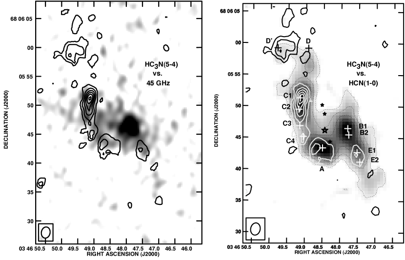
Figure 2.— a) The HC₃N(5–4) integrated intensity map (black line) for IC 342 overlaid on the 7 mm continuum emission (grayscale) extracted from the line free portion of the HC₃N(5–4) datacube. The continuum grayscale ranges from 0.22 mJy bm^-1 - 2.2 mJy bm^-1. HC₃N contours are as in Figure 1. b) The HC₃(5–4) integrated intensity map overlaid on the HCN(1–0) emission (grayscale and dashed contours; Downes et al., 1992). HC₃N contours are as in a). The HCN(1–0) grayscale runs from 0.50 Jy beam km s^-1 to 4 Jy beam km s^-1 and contours are in steps of 0.75 Jy beam km s^-1. Positions of GMC cores (Meier & Turner, 2001) and optical clusters (e.g. Schinnerer et al., 2003, with absolute optical positions having absolute uncertainties of $\sim 1^{{}^{\prime\prime}}$) are labelled.

Figure 3.— The HC₃N(16–15) (thin line) and HC₃N(5–4) (thick line) spectra. Spectra are summed over 2″ apertures centered on each position at the locations of the main GMCs. Note that the bright spectral feature at $\sim$-60 km s^-1 is H₂CO($2_{02}-1_{01}$).

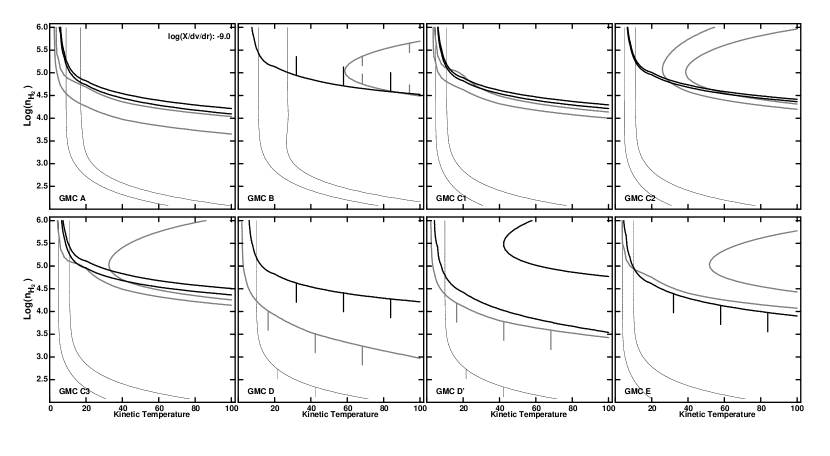
Figure 4.— a) The HC₃N LVG models of the GMCs in IC 342. The thick black lines delineate the observed $\pm 1\sigma$ range of the HC₃N(16–15)/HC₃N(5–4) line ratio (R_16/5), sampled at 2″ resolution. The thick gray lines represents the observed $\pm 1\sigma$ range of the HC₃N(10–9)/HC₃N(5–4) line ratio (R_10/5), sampled at 6″ resolution. $X(HC_{3}N)/dv/dr~{}=~{}10^{-9}$ is assumed for the displayed models. The thin black lines displays the $\pm 1\sigma$ range implied by LVG models of C¹⁸O for comparison (Meier & Turner, 2001). Downward (upward) tickmarks indicate upper (lower) limits.

Figure 5.— HC₃N level population diagrams. Fluxes are taken from a 2${}^{{}^{\prime\prime}}$ box centered on the emission peak. HC₃N(10–9) fluxes are extrapolated from the (5–4) data using the line ratios in Table 1. For each GMC, fitted LVG solutions are displayed for T_K = 10 (solid lines), 30 (dashed lines) and 50 K (dotted lines), except GMC B which includes T_K = 70 K dot-dashed lines) (Table 3). Only models with $X$(HC₃N)/$dv/dr$ = 10^-9 km^-1 s are shown.

References

- Aalto et al. (2002) Aalto, S., Polatidis, A. G., Hüttemeister, S., & Curran, S. J. 2002, A&A, 381, 783
- Aladro et al. (2011) Aladro, R., Martín-Pintado, J., Martín, S., Mauersberger, R., & Bayet, E. 2011, A&A, 525, A89
- Becklin et al. (1980) Becklin, E. E., Gatley, I., Mathews, K., Neugebauer, G., Sellgren, K., Werner, M. K., & Wynn-Williams, C. G.1980, ApJ, 236, 441
- Brandl et al. (2006) Brandl, B. R., et al. 2006, ApJ, 653, 1129
- Bussmann et al. (2008) Bussmann, R. S., et al. 2008, ApJ, 681, L73
- Costagliola & Aalto (2010) Costagliola, F. & Aalto, S., 2010, A&A, 515, 71
- Dahmen et al. (1998) Dahmen, G., Huttemeister, S., Wilson, T. L., & Mauersberger, R. 1998, A&A, 331, 959
- de Vicente et al. (2000) de Vicente, P., Martín-Pintado, J., Neri, R., & Colom, P. 2000, A&A, 361, 1058
- Downes et al. (1992) Downes, D., Radford, S. J. E., Giulloteau, S., Guelin, M., Greve, A., & Morris, D. 1992, A&A, 262, 424
- Fuente et al. (1993) Fuente, A., Martin-Pintado, J., Cernicharo, J., & Bachiller, R. 1993, A&A, 276, 473
- Gao & Solomon (2004) Gao, Y. & Solomon, P. M. 2004, ApJ, 606, 271
- García-Burillo et al. (2000) García-Burillo, S., Martín-Pintado, J., Fuente, A. & Neri, R. 2000, A&A, 355, 499
- García-Burillo et al. (2001) García-Burillo, S., Martín-Pintado, J., Fuente, A. & Neri, R. 2001, ApJ, 563, L27
- García-Burillo et al. (2002) García-Burillo, S., Martín-Pintado, J., Fuente, A., Usero, A. & Neri, R. 2002, ApJ, 575, L55
- Graciá-Carpio et al. (2008) Graciá-Carpio, J., García-Burillo, S., Planesas, P., Fuente, A., & Usero, A. 2008, A&A, 479, 703
- Green & Chapman (1978) Green, S. & Chapman, S. 1978, ApJS, 37, 169
- Harris et al. (1991) Harris, A. I., Hills, R. E., Stutzki, J., Graf, U. U., Russell, A. G. & Genzel, R., 1991, ApJ, 382, L75
- Harrison et al. (1999) Harrison, A., Henkel, C., & Russell, A. 1999, MNRAS, 303, 157
- Ho et al. (1982) Ho, P. T. P., Martin, R. N., & Ruf, K. 1982, A&A, 113, 155
- Hunter et al. (1997) Hunter, S. D. et al. 1997, ApJ, 481, 205
- Ishizuki et al. (1990) Ishizuki, S., Kawabe, R., Ishiguro, M., Okumura, S. K., Morita, K.-I., Chikada, Y., & Kasuga, T. 1990, Nature, 344, 224
- Kennicutt (1998) Kennicutt, R. C., Jr. 1998, ARA&A, 36, 189
- Knudsen et al. (2007) Knudsen, K. K., Walter, F., Weiss, A., Bolatto, A., Riechers, D. A., & Menten, K. 2007, ApJ, 666, 156
- Krips et al. (2008) Krips, M., Neri, R., García-Burillo, S., Martín, S., Combes, F., Graciá-Carpio, J., & Eckart, A. 2008, ApJ, 677, 262
- Karachentsev (2005) Karachentsev, I. D. 2005, AJ, 129, 178
- Lafferty & Lovas (1978) Lafferty, W. J. & Lovas, F. J. 1978, J. Phys. Chem. Ref. Data, 7, 441
- Larson (1981) Larson, R. B. 1981, MNRAS, 194, 809
- Lo et al. (1984) Lo, K. Y. et al. 1984, ApJ, 282, L59
- Maloney & Black (1988) Maloney, P., & Black, J. H. 1988, ApJ, 325, 389
- Mauersberger et al. (1990) Mauersberger, R., Henkel, C. & Sage, L. J. 1990, A&A, 236, 63
- Meier & Turner (2001) Meier, D. S. & Turner, J. L. 2001, ApJ, 551, 687
- Meier & Turner (2004) Meier, D. S., & Turner, J. L. 2004, AJ, 127, 2069
- Meier & Turner (2005) Meier, D. S. & Turner, J. L. 2005, ApJ, 618, 259
- Meier et al. (2000) Meier, D. S., Turner, J. L. & Hurt, R. L. 2000, ApJ, 531, 200
- Meier et al. (2008) Meier, D. S., Turner, J. L., & Hurt, R. L. 2008, ApJ, 675, 281
- Montero-Castaño et al. (2006) Montero-Castaño, M., Herrnstein, R. M., & Ho, P. T. P. 2006, ApJ, 646, 919
- Morris et al. (1976) Morris, M., Turner, B. E., Palmer, P. & Zuckerman, B. 1976, ApJ, 205, 82
- Myers & Benson (1983) Myers, P. C., & Benson, P. J. 1983, ApJ, 266, 309
- Narayanan et al. (2008) Narayanan, D., Cox, T. J., Shirley, Y., Davé, R., Hernquist, L., & Walker, C. K. 2008, ApJ, 684, 996
- Papadopoulos (2007) Papadopoulos, P. P. 2007, ApJ, 656, 792
- Rickard & Harvey (1984) Rickard, L. J, & Harvey, P. M. 1984, AJ, 89, 1520
- Saha et al. (2002) Saha, A., Claver, J. & Hoessel, J. G. 2002, AJ, 124, 839
- Sakamoto (1996) Sakamoto, S. 1996, ApJ, 462, 215
- Schinnerer et al. (2003) Schinnerer, E., Böker, T., & Meier, D. S. 2003, ApJ, 591, L115
- Schinnerer et al. (2008) Schinnerer, E., Böker, T., Meier, D. S., & Calzetti, D. 2008, ApJ, 684, L21
- Schulz et al. (2001) Schulz, A., Güsten, R., Köster, B & Krause, D. 2001, A&A, 371, 25
- Scoville & Sanders (1987) Scoville, N. Z., & Sanders, D. B. 1987, in Interstellar Processes, ed. D. J. Hollenbach and H. A. Thronson, Jr., (Dordrecht: Reidel), 21
- Scoville et al. (1997) Scoville, N. Z., Yun, M. S., & Bryant, P. M. 1997, ApJ, 484, 702
- Smith et al. (1991) Smith, P. A., Brand, P. W. J. L., Mountain, C. M., Puxley, P. J., & Nakai, N. 1991, MNRAS, 252, 6
- Solomon et al. (1987) Solomon, P. M., Rivolo, A. R., Barrett, J., & Yahil, A. 1987, ApJ, 319, 730
- Stark et al. (1989) Stark, A. A., Bally, J., Wilson, R. W., & Pound, M. W. 1989, in The Center of the Galaxy, ed. M. Morris, (Dordrecht: Kluwer), 129
- Strong et al. (1988) Strong, A. W. et al., 1988, A&A, 207, 1
- Tsai et al. (2006) Tsai, C.-W., Turner, J. L., Beck, S. C., Crosthwaite, L. P., Ho, P. T. P. & Meier, D. S. 2006, AJ, in press
- Turner & Ho (1983) Turner, J. L., & Ho, P. T. P. 1983, ApJ, 268, L79
- Turner & Hurt (1992) Turner, J. L., Hurt, R. L. 1992, ApJ, 384, 72
- Turner et al. (1993) Turner, J. L., Hurt, R. L., & Hudson, D. Y. 1993, ApJ, 413, L19
- Usero et al. (2004) Usero, A., García-Burillo, S., Fuente, A., Martín-Pintado, J. & Rodríguez-Fernández, N. J. 2004, A&A, 419, 897
- Usero et al. (2006) Usero, A., García-Burillo, S., Martín-Pintado, J., Fuente, A., & Neri, R. 2006, A&A, 448, 457
- Vanden Bout et al. (1983) Vanden Bout, P. A., Loren, R. B., Snell, R. L. & Wootten, A. 1983, ApJ, 271, 161
- Wall (2007) Wall, W. F. 2007, MNRAS, 379, 674
- Wu et al. (2005) Wu, J., Evans, N. J., II, Gao, Y., Solomon, P. M., Shirley, Y. L., & Vanden Bout, P. A. 2005, ApJ, 635, L173
- Zinchenko et al. (1998) Zinchenko, I., Pirogov, L., & Toriseva, M. 1998, A&AS, 133, 337