Order-preserving factor analysis (OPFA)
Arnau Tibau Puig and Alfred O. Hero III
EECS Department, University of Michigan, Ann Arbor, MI 48109-2122, USA

Order-preserving factor analysis (OPFA)

I Introduction

With the advent of high-throughput data collection techniques, low-dimensional matrix factorizations have become an essential tool for pre-processing, interpreting or compressing high-dimensional data. They are widely used in a variety of signal processing domains including electrocardiogram [1], image [2], or sound [3] processing. These methods can take advantage of a large range of a priori knowledge on the form of the factors, enforcing it through constraints on sparsity or patterns in the factors. However, these methods do not work well when there are unknown misalignments between subjects in the population, e.g., unknown subject-specific time shifts. In such cases, one cannot apply standard patterning constraints without first aligning the data; a difficult task. An alternative approach, explored in this paper, is to impose a factorization constraint that is invariant to factor misalignments but preserves the relative ordering of the factors over the population. This order-preserving factor analysis is accomplished using a penalized least squares formulation using shift-invariant yet order-preserving model selection (group lasso) penalties on the factorization. As a byproduct the factorization produces estimates of the factor ordering and the order-preserving time shifts.

In traditional matrix factorization, the data is modeled as a linear combination of a number of factors. Thus, given an $n\times p$ data matrix $\bm{X}$, the Linear Factor model is defined as:

$$\bm{X}=\bm{M}\bm{A}+\bm{\epsilon},$$ (1)

where $\bm{M}$ is a $n\times f$ matrix of factor loadings or dictionary elements, $\bm{A}$ is a $f\times p$ matrix of scores (also called coordinates) and $\epsilon$ is a small residual. For example, in a gene expression time course analysis, $n$ is the number of time points and $p$ is the number of genes in the study, the columns of $\bm{M}$ contain the features summarizing the genes’ temporal trajectories and the columns of $\bm{A}$ represent the coordinates of each gene on the space spanned by $\bm{M}$. Given this model, the problem is to find a parsimonious factorization that fits the data well according to selected criteria, e.g. minimizing the reconstruction error or maximizing the explained variance. There are two main approaches to such a parsimonious factorization. One, called Factor Analysis, assumes that the number of factors is small and yields a low-rank matrix factorization [4], [5]. The other, called Dictionary Learning [6], [7] or Sparse Coding [8], assumes that the loading matrix $\bm{M}$ comes from an overcomplete dictionary of functions and results in a sparse score matrix $\bm{A}$. There are also hybrid approaches such as Sparse Factor Analysis [1], [9], [2] that try to enforce low rank and sparsity simultaneously.

In many situations, we observe not one but several matrices $\bm{X}_{s}$, $s=1,\cdots,S$ and there are physical grounds for believing that the $\bm{X}_{s}$’s share an underlying model. This happens, for instance, when the observations consist of different time-blocks of sound from the same music piece [3], [10], when they consist of time samples of gene expression microarray data from different individuals inoculated with the same virus [11], or when they arise from the reception of digital data with code, spatial and temporal diversity [12]. In these situations, the fixed factor model (1) is overly simplistic.

An example, which is the main motivation for this work is shown in Figure 1, which shows the effect of temporal misalignment across subjects in a viral challenge study reported in [11]. Figure 1 shows the expression trajectory for a particular gene that undergoes an increase (up-regulation) after viral inoculation at time 0, where the moment when up-regulation occurs differs over the population. Training the model (1) on this data will produce poor fit due to misalignment of gene expression onset times.

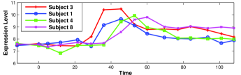
Figure 1: Example of temporal misalignment across subjects of upregulated gene CCRL2. Subject 6 and subject 10 show the earliest and the latest up-regulation responses, respectively.

A more sensible approach for the data in Figure 1 would be to separately fit each subject with a translated version of a common up-regulation factor. This motivates the following extension of model (1), where the factor matrices $\bm{M}_{s}$, $\bm{A}_{s}$ are allowed to vary across observations. Given a number $S$ of $n\times p$ data matrices $\bm{X}_{s}$, we let:

$$\bm{X}_{s}=\bm{M}_{s}\bm{A}_{s}+\bm{\epsilon}_{s} s=1,\cdots,S.$$ (2)

Following the gene expression example, here $n$ is the number of time points, $p$ is the number of genes in the study, and $S$ is the number of subjects participating in the study. Hence, the $n\times f$ matrices $\bm{M}_{s}$ contain the translated temporal features corresponding to the $s$-th subject and the $f\times p$ matrices $\bm{A}_{s}$ accommodate the possibility of subjects having different mixing weights. For different constraints on $\bm{M}_{s}$, $\bm{A}_{s}$, this model specializes to several well-known paradigms such as Principal Components Analysis (PCA) [4], sparse PCA [1], k-SVD [6], structured PCA [2], Non-Negative Matrix Factorization (NNMF) [13], Maximum-Margin Matrix Factorization (MMMF) [14], Sparse Shift-invariant models [3], Parallel Factor Analysis (PARAFAC) [5], [15] or Higher-Order SVD (HOSVD) [16]. Table II summarizes the characteristics of these decomposition models when seen as different instances of the general model (2).

TABLE I: Special cases of the general model (2).

Decomposition	Structure of $\bm{M}_{s}$	Structure of $\bm{A}_{s}$	Uniqueness	Reference
PCA	Orthogonal $\bm{M}_{s}=\bm{F}$	Orthogonal $\bm{A}_{s}$	Yes	SVD
Sparse-PCA	Sparse $\bm{M}_{s}=\bm{F}$	Sparse $\bm{A}_{s}$	No	Sparse PCA [1], [17],
				k-SVD [6], PMD [9]
Structured-PCA	$\bm{M}_{s}=\bm{F}$	Structured Sparse $\bm{A}_{s}$	No	[2]
NNMF	Non-negative $\bm{M}_{s}=\bm{F}$	Non-negative $\bm{A}_{s}$	No	[13]
Sparse	$\bm{M}_{s}=\left[\bm{M}\left(\bm{F},d_{1}\right)\cdots\bm{M}\left(\bm{F},d_{D}\right)\right]$	Sparse $\bm{A}_{s}$	No	[18],
Shift-invariant	where $\left\{d_{j}\right\}_{j=1}^{D}$ are all possible			[3], [10]
models	translations of the $n$-dimensional vectors in $\bm{F}$.
PARAFAC/CP	$\bm{M}_{s}=\bm{F}$	$\bm{A}_{s}=\mbox{diag}\left(\bm{C}_{\cdot,s}\right)\bm{B}^{\prime}$	Yes	[15]
HOSVD	Orthogonal $\bm{M}_{s}=\bm{F}$	$\bm{A}_{s}=\left(\mathcal{G}\times_{3}\bm{C}_{\cdot,s}\right)\bm{B}^{\prime}$	Yes	[16]
		where slices of $\mathcal{G}$
		are orthogonal
OPFA	$\bm{M}_{s}=\bm{M}\left(\bm{F},\bm{d}^{s}\right)$, $\bm{d}^{s}\in\mathcal{K}$	Non-negative,	No	This work.
	where $\bm{F}$ is smooth	sparse $\bm{A}_{s}$
	and non-negative and
	$\mathcal{K}$ enforces consistent
	precedence order

In this paper, we will restrict the columns of $\bm{M}_{s}$ to be translated versions of a common set of factors, where these factors have onsets that occur in some relative order that is consistent across all subjects. Our model differs from previous shift-invariant models considered in [18], [3], [10] in that it restricts the possible shifts to those which preserve the relative order of the factors among different subjects. We call the problem of finding a decomposition (2) under this assumption the Order Preserving Factor Analysis (OPFA) problem.

The contributions of this paper are the following. First, we propose a non-negatively constrained linear model that accounts for temporally misaligned factors and order restrictions. Second, we give a computational algorithm that allows us to fit this model in reasonable time. Finally, we demonstrate that our methodology is able to succesfully extract the principal features in a simulated dataset and in a real gene expression dataset. In addition, we show that the application of OPFA produces factors that can be used to significantly reduce the variability in clustering of gene expression responses.

This paper is organized as follows. In Section II we present the biological problem that motivates OPFA and introduce our mathematical model. In Section III, we formulate the non-convex optimization problem associated with the fitting of our model and give a simple local optimization algorithm. In Section IV we apply our methodology to both synthetic data and real gene expression data. Finally we conclude in Section V. For lack of space many technical details are left out of our presentation but are available in the accompanying technical report [19].

II Motivation: gene expression time-course data

In this section we motivate the OPFA mathematical model in the context of gene expression time-course analysis. Temporal profiles of gene expression often exhibit motifs that correspond to cascades of up-regulation/down-regulation patterns. For example, in a study of a person’s host immune response after inoculation with a certain pathogen, one would expect genes related to immune response to exhibit consistent patterns of activation across pathogens, persons, and environmental conditions.

A simple approach to characterize the response patterns is to encode them as sequences of a few basic motifs such as (see, for instance, [20]):

• Up-regulation: Gene expression changes from low to high.

• Down-regulation: Gene expression changes from a high to a low level.

• Steady: Gene expression does not vary.

If gene expression is coherent over the population of several individuals, e.g., in response to a common viral insult, the response patterns can be expected to show some degree of consistency across subjects. Human immune system response is a highly evolved system in which several biological pathways are recruited and organized over time. Some of these pathways will be composed of genes whose expressions obey a precedence-ordering, e.g., virally induced ribosomal protein production may precede toll-like receptor activation and antigen presentation [21]. This consistency exists despite temporal misalignment: even though the order is preserved, the specific timing of these events can vary across the individuals. For instance, two different persons can have different inflammatory response times, perhaps due to a slower immune system in one of the subjects. This precedence-ordering of motifs in the sequence of immune system response events is invariant to time shifts that preserve the ordering. Thus if a motif in one gene precedes another motif in another gene for a few subjects, we might expect the same precedence relationship to hold for all other subjects. Figure 2 shows two genes from [11] whose motif precedence-order is conserved across 3 different subjects. This conservation of order allows one to impose ordering constraints on (2) without actually knowing the particular order or the particular factors that obey the order-preserving property.

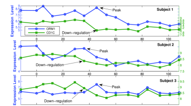
Figure 2: Example of gene patterns with a consistent precedence-order across 3 subjects. The down-regulation motif of gene CD1C precedes the peak motif of gene ORM1 across these three subjects.

Often genes are co-regulated or co-expressed and have highly correlated expression profiles. This can happen, for example, when the genes belong to the same signaling pathway. Figure 3 shows a set of different genes that exhibit a similar expression pattern (up-regulation motif). The existence of high correlation between large groups of genes allows one to impose a low rank property on the factorization in (2).

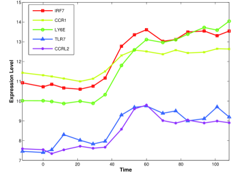
Figure 3: Example of gene patterns exhibiting co-expression for a particular subject in the viral challenge study in [11].

In summary, our OPFA model is based on the following assumptions:

• A1: Motif consistency across subjects: Gene expression patterns have consistent (though not-necessarily time aligned) motifs across subjects undergoing a similar treatment.

• A2: Motif sequence consistency across subjects: If motif $X$ precedes motif $Y$ for subject $s$, the same precedence must hold for subject $t\neq s$.

• A3: Motif consistency across groups of genes: There are (not necessarily known) groups of genes that exhibit the same temporal expression patterns for a given subject.

• A4: Gene Expression data is non-negative: Gene expression on a microarray is measured as an abundance and standard normalization procedures, such as RMA [22], preserve the non-negativity of this measurement.

A few microarray normalization software packages produce gene expression scores that do not satisfy the non-negativity assumption A4. In such cases, the non-negativity constraint in the algorithm implementing (9) can be disabled. Note that in general, only a subset of genes may satisfy assumptions A1-A3.

III OPFA mathematical model

In the OPFA model, each of the $S$ observations is represented by a linear combination of temporally aligned factors. Each observation is of dimension $n\times p$, where $n$ is the number of time points and $p$ is the number of genes under consideration. Let $\bm{F}$ be an $n\times f$ matrix whose columns are the $f$ common alignable factors, and let $\bm{M}\left(\bm{F},\bm{d}\right)$ be a matrix valued function that applies a circular shift to each column of $\bm{F}$ according to the vector of shift parameters $\bm{d}$, as depicted in Figure 12. Then, we can refine model (2) by restricting ${\mathbf{M}}_{s}$ to have the form:

$$\bm{M}_{s}=\bm{M}\left(\bm{F},\bm{d}^{s}\right).$$ (3)

where $\bm{d}^{s}\in\left\{0,\cdots,d_{\max}\right\}^{f}$ and $d_{\max}\leq n$ is the maximum shift allowed in our model. This model is a generalization of a simpler one that restricts all factors to be aligned but with a common delay:

$$\bm{M}_{s}=\bm{U}_{s}\bm{F},$$ (4)

where $\bm{U}_{s}$ is a circular shift operator. Specifically, the fundamental characteristic of our model (3) is that each column can have a different delay, whereas (4) is a restriction of (3) with $d^{s}_{i}=d^{s}_{j}$ for all $s$ and all $i$, $j$.

The circular shift is not restrictive. By embedding the observation into a larger time window it can accommodate transient gene expression profiles in addition to periodic ones, e.g., circadian rhythms [19]. There are several ways to do this embedding. One way is to simply extrapolate the windowed, transient data to a larger number of time points $n_{F}=n+d_{\max}$. This is the strategy we follow in the numerical experiments of Section IV-B.

Figure 4: Each subject’s factor matrix $\bm{M}_{s}$ is obtained by applying a circular shift to a common set of factors $\bm{F}$ parameterized by a vector $\bm{d}$.

This alignable factor model parameterizes each observation’s intrinsic temporal dynamics through the $f$-dimensional vector $\bm{d}^{s}$. The precedence-ordering constraint A2 is enforced by imposing the condition

$$d_{j_{1}}^{s_{1}}\leq d_{j_{2}}^{s_{1}}\Leftrightarrow d_{j_{1}}^{s_{2}}\leq d_{j_{2}}^{s_{2}}\mbox{ }\forall s_{2}\neq s_{1},$$ (5)

that is, if factor $j_{1}$ precedes factor $j_{2}$ in subject $s_{1}$, then the same ordering will hold in all other subjects. Since the indexing of the factors is arbitrary, we can assume without loss of generality that $d_{i}^{s}\leq d_{i+1}^{s}$ for all $i$ and all $s$. This characterization constrains each observation’s delays $\bm{d}^{s}$ independently, allowing for a computationally efficient algorithm for fitting model (3).

III-A Relationship to 3-way factor models.

Our proposed OPFA framework is significantly different from other factor analysis methods and these differences are illustrated in the simulated performance comparisons below. However, there are some similarities, especially to 3-way factor models [15], [23] that are worth pointing out.

An $n$-th order tensor or $n$-way array is a data structure whose elements are indexed by an $n$-tuple of indices [23]. $n$-way arrays can be seen as multidimensional generalizations of vectors and matrices: an $1$-way array is a vector and a $2$-way array is a matrix. Thus, we can view our observations $\bm{X}_{s}$ as the slices of a third order tensor $\mathcal{X}$ of dimension $p\times n\times S$: $\bm{X}_{s}=\mathcal{X}_{\cdot,\cdot,i}$. Tensor decompositions aim at extending the ideas of matrix (second order arrays) factorizations to higher order arrays [15], [23] and have found many applications in signal processing and elsewhere [23], [15], [16], [12], [24]. Since our data tensor is of order 3, we will only consider here 3-way decompositions, which typically take the following general form:

$$\mathcal{X}_{i,j,k}=\sum_{p=1}^{P}\sum_{q=1}^{Q}\sum_{r=1}^{R}{\mathcal{G}}_{pqr}\bm{F}_{ip}\bm{B}_{jq}\bm{C}_{kr}$$ (6)

where $P$, $Q$, $R$ are the number of columns in each of the factor matrices $\bm{F}$, $\bm{B}$, $\bm{C}$ and $\mathcal{G}$ is a $P\times Q\times R$ tensor. This class of decompositions is known as the Tucker model. When orthogonality is enforced among $\bm{F}$, $\bm{B}$, $\bm{C}$ and different matrix slices of $\mathcal{G}$, one obtains the Higher Order SVD [16]. When $\mathcal{G}$ is a superdiagonal tensor and $P=Q=R$, this model amounts to the PARAFAC/Canonical Decomposition (CP) model [5], [12], [24]. The PARAFAC model is the closest to OPFA. Under this model, the slices of $\mathcal{X}_{i,j,k}$ can be written as:

$$\bm{X}^{\mbox{CP}}_{s}=\bm{F}\mbox{diag}\left(\bm{C}_{\cdot,s}\right)\bm{B}^{\prime}.$$ (7)

This expression is to be compared with our OPFA model, which we state again here for convenience:

$$\bm{X}^{\mbox{OPFA}}_{s}=\bm{M}\left(\bm{F},\bm{d}^{s}\right)\bm{A}_{s}.$$ (8)

Essentially, (7) shows that the PARAFAC decomposition is a special case of the OPFA model (8) where the factors are fixed ($\bm{M}_{s}=\bm{F}$) and the scores only vary in magnitude across observations ($\bm{A}_{s}=\mbox{diag}\left(\bm{C}_{\cdot,s}\right)\bm{B}^{\prime}$). This structure enhances uniqueness (under some conditions concerning the linear independence of the vectors in $\bm{F}$, $\bm{B}$, $\bm{C}$, see [15]) but lacks the additional flexibility necessary to model possible translations in the columns of the factor matrix $\bm{F}$. If $\bm{d}^{s}=\bm{0}$ for all $s$, then the OPFA (8) and the Linear Factor model (1) also coincide. The OPFA model can be therefore seen as an extension of the Linear Factor and PARAFAC models where the factors are allowed to experiment order-preserving circular translations across different individuals.

III-B OPFA as an optimization problem

OPFA tries to fit the model (2)-(5) to the data $\left\{\bm{X}_{s}\right\}_{s=1}^{S}$. For this purpose, we define the following penalized and constrained least squares problem:

$$\min \sum_{s=1}^{S}\left|\left|\bm{X}_{s}-\bm{M}\left(\bm{F},\bm{d}^{s}\right)\bm{A}_{s}\right|\right|_{F}^{2}+\lambda P_{1}\left(\bm{A}_{1},\cdots,\bm{A}_{S}\right)+\beta P_{2}\left(\bm{F}\right)$$ (9)

s.t. $$\left\{\bm{d}^{s}\right\}_{s}\in{\mathcal{K}},\bm{F}\in{\mathcal{F}},\bm{A}_{s}\in{\mathcal{A}}_{s}$$

where $\left|\left|\cdot\right|\right|_{F}$ is the Frobenius norm, $\lambda$ and $\beta$ are regularization parameters, and the set $\mathcal{K}$ constrains the delays $\bm{d}^{s}$ to be order-preserving:

$${\mathcal{K}}=\left\{\bm{d}\in\left\{0,\cdots,d_{\max}\right\}^{f}:{d}_{i+1}\geq{d}_{i},\forall i\right\}.$$ (10)

where $d_{\max}\leq n$. The other soft and hard constraints are briefly described as follows.

For the gene expression application we wish to extract factors $\bm{F}$ that are smooth over time and non-negative. Smoothness will be captured by the constraint that $P_{2}(\bm{F})$ is small where $P_{2}(\bm{F})$ is the squared total variation operator

$$P_{2}\left(\bm{F}\right)=\sum_{i=1}^{f}\left|\left|\bm{W}\bm{F}_{\cdot,i}\right|\right|_{2}^{2}$$ (11)

where $\bm{W}$ is an appropriate weighting matrix and $\bm{F}_{\cdot,i}$ denotes the $i$-th column of matrix $\bm{F}$. From A4, the data is non-negative and hence non-negativity is enforced on $\bm{F}$ and the loadings $\bm{A}_{s}$ to avoid masking of positive and negative valued factors whose overall contribution sums to zero. To avoid numerical instability associated with the scale invariance $\bm{M}\bm{A}=\frac{1}{\alpha}\bm{M}\alpha\bm{A}$ for any $\alpha>0$, we constrain the Frobenius norm of $\bm{F}$. This leads to the following constraint sets:

$${\mathcal{F}}=\left\{\bm{F}\in{\mathbb{R}}_{+}^{n\times f}:\left|\left|\bm{F}\right|\right|_{F}\leq\delta\right\}$$ (12)

$${\mathcal{A}}_{s}={\mathbb{R}}_{+}^{f\times p},s=1,\cdots,S$$

The parameter $\delta$ above will be fixed to a positive value as its purpose is purely computational and has little practical impact. Since the factors $\bm{F}$ are common to all subjects, assumption A3 requires that the number of columns of $\bm{F}$ (and therefore, its rank) is small compared to the number of genes $p$. In order to enforce A1 we consider two different models. In the first model, which we shall name OPFA, we constrain the columns of $\bm{A}_{s}$ to be sparse and the sparsity pattern to be consistent across different subjects. Notice that A1 does not imply that the mixing weights $\bm{A}_{s}$ are the same for all subjects as this would not accommodate magnitude variability across subjects. We also consider a more restrictive model where we constrain $\bm{A}_{1}=\cdots=\bm{A}_{S}=\bm{A}$ with sparse $\bm{A}$ and we call this model OPFA-C, the C standing for the additional constraint that the subjects share the same sequence ${\mathbf{A}}$ of mixing weights. The OPFA-C model has a smaller number of parameters than OPFA, possibly at the expense of introducing bias with respect to the unconstrained model. A similar constraint has been succesfully adopted in [25] in a factor model for multi-view learning.

Similarly to the approach taken in [26] in the context of simultaneous sparse coding, the common sparsity pattern for OPFA is enforced by constraining $P_{1}\left(\bm{A}_{1},\cdots,\bm{A}_{S}\right)$ to be small, where $P_{1}$ is a mixed-norm group-Lasso type penalty function [27]. For each of the $p\times f$ score variables, we create a group containing its $S$ different values across subjects:

$$P_{1}\left(\bm{A}_{1},\cdots,\bm{A}_{S}\right)=\sum_{i=1}^{p}\sum_{j=1}^{f}\|\left[\bm{A}_{1}\right]_{j,i}\cdots\left[\bm{A}_{S}\right]_{j,i}\|_{2}.$$ (13)

Table II summarizes the constraints of each of the models considered in this paper.

Following common practice in factor analysis, the non-convex problem (9) is addressed using Block Coordinate Descent, displayed in the figure labeled Algorithm 1, which iteratively minimizes (9) with respect to the shift parameters $\{\bm{d}^{s}\}_{s=1}^{S}$, the scores $\{\bm{A}_{s}\}_{s=1}^{S}$ and the factors $\bm{F}$ while keeping the other variables fixed. This algorithm is guaranteed to monotonically decrease the objective function at each iteration. Since both the Frobenius norm and $P_{1}\left(\cdot\right)$, $P_{2}\left(\cdot\right)$ are non-negative functions, this ensures that the algorithm converges to a (possibly local) minima or a saddle point of (9).

Input: Initial estimate of $\bm{F}$ and $\left\{\bm{A}_{s}\right\}_{s=1}^{S}$, $\epsilon$, $\lambda$, $\beta$.

Output: $\bm{F}$, $\left\{\bm{A}_{s}\right\}_{s=1}^{S}$, $\left\{\bm{d}^{s}\right\}_{s=1}^{S}$

$c^{0}=\infty$

$c^{1}\leftarrow\mbox{OPFAObjective}\left(\bm{F},\left\{\bm{A}_{s}\right\}_{s=1}^{S},\left\{\bm{d}^{s}\right\}_{s=1}^{S}\right)$

$t=1$

while $c^{t-1}-c^{t}\geq\epsilon$ do

       $~{}~{}\left\{\bm{d}^{s}\right\}_{s=1}^{S}\leftarrow\mbox{EstimateDelays}\left(\bm{F},\left\{\bm{A}_{s}\right\}_{s=1}^{S}\right)$

       $~{}~{}\left\{\bm{A}_{s}\right\}_{s=1}^{S}\leftarrow\mbox{EstimateScores}\left(\bm{F},\left\{\bm{d}^{s}\right\}_{s=1}^{S}\right)$

       $~{}~{}\bm{F}\leftarrow\mbox{EstimateFactors}\left(\left\{\bm{A}_{s}\right\}_{s=1}^{S},\left\{\bm{d}^{s}\right\}_{s=1}^{S}\right)$

       $~{}~{}c^{t}\leftarrow\mbox{OPFAObjective}\left(\bm{F},\left\{\bm{A}_{s}\right\}_{s=1}^{S},\left\{\bm{d}^{s}\right\}_{s=1}^{S}\right)$

       $~{}~{}t\leftarrow t+1$

Algorithm 1 BCD algorithm for finding a local minima of (9). $\mbox{OPFAObjective}\left(\bm{F},\left\{\bm{A}_{s}\right\}_{s=1}^{S},\left\{\bm{d}^{s}\right\}_{s=1}^{S}\right)$ denotes the objective function in (9)

The subroutines EstimateFactors and EstimateScores solve the following penalized regression problems:

$$\min_{\bm{F}} \sum_{s=1}^{S}\left|\left|\bm{X}_{s}-\bm{M}\left(\bm{F},\bm{d}^{s}\right)\bm{A}_{s}\right|\right|_{F}^{2}+\beta\sum_{i=1}^{f}\left|\left|\bm{W}\bm{F}_{\cdot,i}\right|\right|_{2}^{2}$$ (14)

s.t. $$\left\{\begin{array}[]{c c}\left|\left|\bm{F}\right|\right|^{2}_{\mathcal{F}}\leq\delta&\\ \bm{F}_{i,j}\geq 0&i=1,\cdots,n,\\ &j=1,\cdots,f\end{array}\right.$$ (17)

and

$$\min_{\left\{\bm{A}_{s}\right\}_{s=1}^{S}} \sum_{s=1}^{S}\left|\left|\bm{X}_{s}-\bm{M}\left(\bm{F},\bm{d}^{s}\right)\bm{A}_{s}\right|\right|_{F}^{2}+\lambda\sum_{i=1}^{p}\sum_{j=1}^{f}\|\left[\bm{A}_{1}\right]_{j,i}\cdots\left[\bm{A}_{S}\right]_{j,i}\|_{2}$$ (18)

s.t. $$\left\{\begin{array}[]{l c}\left[\bm{A}_{s}\right]_{j,i}\geq 0&i=1,\cdots,n,\\ &j=1,\cdots,f,\\ &s=1,\cdots,S\end{array}\right.$$ (22)

Notice that in OPFA-C, we also incorporate the constraint $\bm{A}_{1}=\cdots=\bm{A}_{S}$ in the optimization problem above. The first is a convex quadratic problem with a quadratic and a linear constraint over a domain of dimension $fn$. In the applications considered here, both $n$ and $f$ are small and hence this problem can be solved using any standard convex optimization solver. EstimateScores is trickier because it involves a non-differentiable convex penalty and the dimension of its domain is equal to $Sfp$, where $p$ can be very large. In our implementation, we use an efficient first-order method [28] designed for convex problems involving a quadratic term, a non-smooth penalty and a separable constraint set. These procedures are described in more detail in Appendix -C and therefore we focus on the EstimateDelays subroutine. EstimateDelays is a discrete optimization that is solved using a branch-and-bound (BB) approach [29]. In this approach a binary tree is created by recursively dividing the feasible set into subsets (“branch”). On each of the nodes of the tree lower and upper bounds (“bound”) are computed. When a candidate subset is found whose upper bound is less than the smallest lower bound of previously considered subsets these latter subsets can be eliminated (“prune”) as candidate minimizers. Whenever a leaf (singleton subset) is obtained, the objective is evaluated at the corresponding point. If its value exceeds the current optimal value, the leaf is rejected as a candidate minimizer, otherwise the optimal value is updated and the leaf included in the list of candidate minimizers. Details on the application of BB to OPFA are given below.

The subroutine EstimateDelays solves $S$ uncoupled problems of the form:

$$\min_{\bm{d}\in\mathcal{K}}\left|\left|{\bm{X}_{s}}-\bm{M}\left(\bm{F},\bm{d}\right)\bm{A}_{s}\right|\right|^{2}_{F},$$ (23)

where the set $\mathcal{K}$ is defined in (10). The “branch” part of the optimization is accomplished by recursive splitting of the set $\mathcal{K}$ to form a binary tree. The recursion is initialized by setting ${\mathcal{S}}_{o}=\left\{0,\cdots,d_{\max}\right\}^{f}$, ${\mathcal{I}}_{o}=\left\{\bm{d}\in{\mathcal{K}}\cap{\mathcal{S}}_{o}\right\}$. The splitting of the set ${\mathcal{I}}_{o}$ into two subsets is done as follows

$${\mathcal{I}}_{1} = \left\{\bm{d}\in{\mathcal{K}}\cap{\mathcal{S}}_{o}:d_{\omega_{1}}\leq\gamma_{1}\right\}$$ (24)

$${\mathcal{I}}_{2} = \left\{\bm{d}\in{\mathcal{K}}\cap{\mathcal{S}}_{o}:d_{\omega_{1}}>\gamma_{1}\right\},$$

and we update ${\mathcal{S}}_{1}=\left\{\bm{d}\in{\mathcal{S}}_{o}:d_{\omega_{1}}\leq\gamma_{1}\right\}$, ${\mathcal{S}}_{2}=\left\{\bm{d}\in{\mathcal{S}}_{o}:d_{\omega_{1}}>\gamma_{1}\right\}$. Here $\gamma_{1}$ is an integer $0\leq\gamma_{1}\leq d_{\max}$, and $\omega_{1}\in\left\{1,\cdots,f\right\}$. ${\mathcal{I}}_{1}$ contains the elements $\bm{d}\in{\mathcal{K}}$ whose $\omega_{1}$-th component is strictly larger than $\gamma_{1}$ and ${\mathcal{I}}_{2}$ contains the elements whose $\omega_{1}$-th component is smaller than $\gamma_{1}$. The same kind of splitting procedure is then subsequently applied to ${\mathcal{I}}_{1}$, ${\mathcal{I}}_{2}$ and its resulting subsets. After $k-1$ successive applications of this decomposition there will be $2^{k-1}$ subsets and the $k$-th split will be :

$${\mathcal{I}}_{t}:= \left\{\bm{d}\in{\mathcal{K}}\cap{\mathcal{S}}_{t}\right\}$$ (25)

$${\mathcal{I}}_{t+1}:= \left\{\bm{d}\in{\mathcal{K}}\cap{\mathcal{S}}_{t+1}\right\}$$

where

$${\mathcal{S}}_{t}=\left\{\bm{d}\in{\mathcal{S}}_{\pi_{k}}:d_{\omega_{k}}\leq\gamma_{k}\right\}$$

$${\mathcal{S}}_{t+1}=\left\{\bm{d}\in{\mathcal{S}}_{\pi_{k}}:d_{\omega_{k}}>\gamma_{k}\right\}.$$

and $\pi_{k}\in\left\{1,\cdots,2^{k-1}\right\}$ denotes the parent set of the two new sets $t$ and $t+1$, i.e. $\mbox{pa}(t)=\pi_{k}$ and $\mbox{pa}(t+1)=\pi_{k}$. In our implementation the splitting coordinate $\omega_{k}$ is the one corresponding to the coordinate in the set ${\mathcal{I}}_{\pi_{k}}$ with largest interval. The decision point $\gamma_{k}$ is taken to be the middle point of this interval.

The “bound” part of the optimization is as follows. Denote $g\left(\bm{d}\right)$ the objective function in (23) and define its minimum over the set ${\mathcal{I}}_{t}\subset\mathcal{K}$:

$$g_{\min}\left({\mathcal{I}}_{t}\right)=\min_{\bm{d}\in{\mathcal{I}}_{t}}g\left(\bm{d}\right).$$ (26)

A lower bound for this value can be obtained by relaxing the constraint $\bm{d}\in\mathcal{K}$ in (25):

$$\min_{\bm{d}\in{\mathcal{S}}_{t}}g\left(\bm{d}\right)\leq g_{\min}\left({\mathcal{I}}_{t}\right)$$ (27)

Letting $\bm{X}_{s}=\bm{X}_{s}^{\perp}+\bm{X}_{s}^{\parallel}$ where $\bm{X}_{s}^{\parallel}=\bm{X}_{s}\bm{A}_{s}^{{\dagger}}\bm{A}_{s}$ and $\bm{X}_{s}^{\perp}=\bm{X}_{s}\left(\bm{I}-\bm{A}_{s}^{{\dagger}}\bm{A}_{s}\right)$, we have:

$$\left|\left|{\bm{X}_{s}}-\bm{M}\left(\bm{F},\bm{d}\right)\bm{A}_{s}\right|\right|^{2}_{F} =\left|\left|\left({\bm{X}_{s}}\bm{A}_{s}^{{\dagger}}-\bm{M}\left(\bm{F},\bm{d}\right)\right)\bm{A}_{s}\right|\right|^{2}_{F}$$

$$+\left|\left|{\bm{X}_{s}}^{\perp}\right|\right|^{2}_{F},$$

where $\bm{A}_{s}^{{\dagger}}$ denotes the pseudoinverse of $\bm{A}_{s}$. This leads to:

$$\underline{\lambda}\left(\bm{A}_{s}\bm{A}_{s}^{T}\right)\left|\left|{\bm{X}_{s}}\bm{A}_{s}^{{\dagger}}-\bm{M}\left(\bm{F},\bm{d}\right)\right|\right|^{2}_{F}+\left|\left|{\bm{X}_{s}}^{\perp}\right|\right|^{2}_{F}\leq g\left(\bm{d}\right),$$ (28)

where $\underline{\lambda}\left(\bm{A}_{s}\bm{A}_{s}^{T}\right)$ denotes the smallest eigenvalue of the symmetric matrix $\bm{A}_{s}\bm{A}_{s}^{T}$. Combining the relaxation in (27) with inequality (28), we obtain a lower bound on $g_{\min}\left({\mathcal{I}}_{t}\right)$:

$$\Phi_{lb}\left({\mathcal{I}}_{t}\right) ={\min}_{\bm{d}\in{\mathcal{S}}_{t}}\underline{\lambda}\left(\bm{A}_{s}\bm{A}_{s}^{T}\right)\left|\left|{\bm{X}_{s}}\bm{A}_{s}^{{\dagger}}-\bm{M}\left(\bm{F},\bm{d}\right)\right|\right|_{F}^{2}$$ (29)

$$+\left|\left|{\bm{X}_{s}}^{\perp}\right|\right|^{2}_{F}$$

$$\leq g_{\min}\left({\mathcal{I}}_{t}\right),$$

which can be evaluated by performing $f$ decoupled discrete grid searches. At the $k$-th step, the splitting node $\pi_{k}$ will be chosen as the one with smallest $\Phi_{lb}\left({\mathcal{I}}_{t}\right)$. Finally, this lower bound is complemented by the upper bound

$$g_{\min}\left({\mathcal{I}}_{t}\right)\leq\Phi_{ub}\left({\mathcal{I}}_{t}\right)=g\left(\bm{d}\right)\mbox{ for }\forall\bm{d}\in{\mathcal{I}}_{t}.$$ (30)

These bounds enable the branch-and-bound optimization of (23).

III-C Selection of the tuning parameters $f$, $\lambda$ and $\beta$

From (9), it is clear that the OPFA factorization depends on the choice of $f$, $\lambda$ and $\beta$. This is a paramount problem in unsupervised learning, and several heuristic approaches have been devised for simpler factorization models [30, 31, 9]. These approaches are based on training the factorization model on a subset of the elements of the data matrix (training set) to subsequently validate it on the excluded elements (test set).

The variational characterization of the OPFA decomposition allows for the presence of missing variables, i.e. missing elements in the observed matrices $\left\{\bm{X}_{s}\right\}_{s=1}^{S}$. In such case, the Least Squares fitting term in (9) is only applied to the observed set of indices. We will hence follow the approach in [9] and train the OPFA model over a fraction $1-\delta$ of the entries in the observations $\bm{X}_{s}$. Let $\Omega_{s}$ denote the set of $\delta\left(n\times p\right)$ excluded entries for the $s$-th observation. These entries will constitute our test set, and thus our Cross-Validation error measure is:

$$\mbox{CV}\left(f,\lambda,\beta\right)=\frac{1}{S}\sum_{s=1}^{S}\left|\left|\left[\bm{X}_{s}-\bm{M}\left(\hat{\bm{F}},\hat{\bm{d}}^{s}\right)\hat{\bm{A}}_{s}\right]_{\Omega_{s}}\right|\right|_{F}^{2}$$

where $\hat{\bm{F}},\left\{\hat{\bm{d}}^{s}\right\}_{s=1}^{S},\left\{\hat{\bm{A}}_{s}\right\}_{s=1}^{S}$ are the OPFA estimates obtained on the training set excluding the entries in $\left\{\Omega_{s}\right\}_{s=1}^{S}$, for a given choice of $f$, $\lambda$, and $\beta$.

IV Numerical results

IV-A Synthetic data: Periodic model

First we evaluate the performance of the OPFA algorithm for a periodic model observed in additive Gaussian white noise:

$$\bm{X}_{s}=\bm{M}\left(\bm{F},\bm{d}^{s}\right)\bm{A}_{s}+\epsilon_{s} s=1,\ldots,S.$$ (31)

Here $\epsilon_{s}\sim{\mathcal{N}}_{n\times p}\left(\bm{0},\sigma_{\epsilon}^{2}\bm{I}\right)$, $\bm{d}^{s}=\mbox{sort}\left(\bm{t}^{s}\right)$ where $\sigma_{\epsilon}^{2}$ is the variance of $\epsilon_{s}$ and $\bm{t}^{s}\sim{\mathcal{U}}\left(0,\sqrt{12\sigma_{d}^{2}+1}\right)$ are i.i.d. The $f=2$ columns of $\bm{F}$ are non-random smooth signals from the predefined dictionary shown in Figure 5. The scores $\bm{A}_{s}$ are generated according to a consistent sparsity pattern across all subjects and its non zero elements are i.i.d. normal truncated to the non-negative orthant.

TABLE II: Models considered in Section IV-A.

Model	$\bm{M}_{s}$	$\bm{A}_{s}$
OPFA	$\bm{M}_{s}=\bm{M}\left(\bm{F},\bm{d}^{s}\right)$	Non-negative
	$\bm{d}^{s}\in\mathcal{K}$, $\bm{F}$ smooth	sparse $\bm{A}_{s}$
	and non-negative
OPFA-C	$\bm{M}_{s}=\bm{M}\left(\bm{F},\bm{d}^{s}\right)$	Non-negative
	$\bm{d}^{s}\in\mathcal{K}$, $\bm{F}$ smooth	sparse
	and non-negative	$\bm{A}_{1}=\cdots=\bm{A}_{S}$
SFA	$\bm{M}_{s}=\bm{M}\left(\bm{F},\bm{d}^{s}\right)$,	Non-negative
	$\bm{d}^{s}=\bm{0}$ ,$\bm{F}$ smooth	sparse $\bm{A}_{s}$
	and non-negative

Figure 5: Dictionary used to generated the 2-factor synthetic data of Section IV.

Here the number of subjects is $S=10$, the number of variables is $p=100$, and the number of time points is $n=20$. In these experiments experiments we choose to initialize the factors $\bm{F}$ with temporal profiles obtained by hierarchical clustering of the data. Hierarchical clustering [32] is a standard unsupervised learning technique that groups the $p$ variables into increasingly finer partitions according to the normalized euclidean distance of their temporal profiles. The average expression patterns of the clusters found are used as initial estimates for $\bm{F}$. The loadings $\left\{\bm{A}_{s}\right\}_{s=1}^{S}$ are initialized by regressing the obtained factors onto the data.

We compare OPFA and OPFA-C to a standard Sparse Factor Analysis (SFA) solution, obtained by imposing $d_{\max}=0$ in the original OPFA model. Table II summarizes the characteristics of the three models considered in the simulations. We fix $f=2$ and choose the tuning parameters $\left(\lambda,\beta\right)$ using the Cross-Validation procedure of Section III-C with a $5\times 3$ grid and $\delta=.1$.

In these experiments, we consider two measures of performance, the Mean Square Error (MSE) with respect to the generated data:

$$MSE:=\frac{1}{S}\sum_{s=1}^{S}E\left|\left|\bm{D}_{s}-\hat{\bm{D}}_{s}\right|\right|_{F}^{2},$$

where $E$ is the expectation operator, $\bm{D}_{s}=\bm{M}\left(\bm{F},\bm{d}^{s}\right)\bm{A}_{s}$ is the generated noiseless data and $\hat{\bm{D}}_{s}=\bm{M}\left(\hat{\bm{F}},\hat{\bm{d}}^{s}\right)\hat{\bm{A}}_{s}$ is the estimated data, and the Distance to the True Factors (DTF), defined as:

$$DTF:=1-\frac{1}{f}\sum_{i=1}^{f}E\frac{\bm{F}_{\cdot,i}^{T}\hat{\bm{F}}_{\cdot,i}}{\left|\left|\bm{F}_{\cdot,i}\right|\right|_{2}\left|\left|\hat{\bm{F}}_{\cdot,i}\right|\right|_{2}},$$

where $\bm{F}$, $\hat{\bm{F}}$ are the generated and the estimated factor matrices, respectively.

Figure 6 shows the estimated MSE and DTF performance curves as a function of the delay variance $\sigma_{d}^{2}$ for fixed SNR$=15$dB (which is defined as $SNR=10\log\left(\frac{1}{S}\sum_{s}\frac{E\left(\left|\left|\bm{M}\left(\bm{F},\bm{d}^{s}\right)\bm{A}_{s}\right|\right|^{2}_{F}\right)}{np\sigma_{\epsilon}^{2}}\right)$). OPFA and OPFA-C perform at least as well as SFA for zero delay ($\sigma_{d}=0$) and significantly better for $\sigma_{d}>0$ in terms of DTF. OPFA-C outperforms OPFA for high delay variances $\sigma_{d}^{2}$ at the price of a larger MSE due to the bias introduced by the constraint $\bm{A}_{1}=\cdots=\bm{A}_{S}$. In Figure 7 the performance curves are plotted as a function of SNR, for fixed $\sigma_{d}^{2}=5$. Note that OPFA and OPFA-C outperform SFA in terms of DTF and that OPFA is better than the others in terms of MSE for SNR$>0$db. Again, OPFA-C shows increased robustness to noise in terms of DTF.

We also performed simulations to demonstrate the value of imposing the order-preserving constraint in (23). This was accomplished by comparing OPFA to a version of OPFA for which the constraints in (23) are not enforced. Data was generated according to the model (31) with $S=4$, $n=20$, $f=2$, and $\sigma_{d}^{2}=5$. The results of our simulations (not shown) were that, while the order-preserving constraints never degrade OPFA performance, the constraints improve performance when the SNR is small (below 3dB for this example).

Finally, we conclude this sub-section by studying the sensitivity of the final OPFA estimates with respect to the initialization choice. To this end, we initialize the OPFA algorithm with the correct model perturbed with a random gaussian vector of increasing variance. We analyze the performance of the estimates in terms of MSE and DTF as a function of the norm of the model perturbation relative to the norm of the noiseless data, which we denote by $\rho$. Notice that larger $\rho$ corresponds to increasingly random initialization. The results in Table III show that the MSE and DTF of the OPFA estimates are very similar for a large range of values of $\rho$, and therefore are robust to the initialization.

TABLE III: Sensitivity of the OPFA estimates to the initialization choice with respect to the relative norm of the perturbation ($\rho$).

	DTF [ mean (standard deviation) ] $\times 10^{-3}$
SNR	$\rho=0.002$	$\rho=1.08$	$\rho=53.94$
$22.8$	$0.0$ ($0.0$)	$3.4$ ($9.4$)	$1.9$ ($3.2$)
$-2$	$1.3$ ($0.5$)	$1$ ($9.4$)	$1.25$ ($1.5$)
$-27.1$	$46$ ($20$)	$58$ ($17$)	$63$ ($8$)

	MSE [ mean (standard deviation $\times 10^{-3}$) ]
SNR	$\rho=0.002$	$\rho=1.08$	$\rho=53.94$
$22.8$	$0.02$ ($1.5$)	$0.05$ ($69$)	$0.11$ ($99$)
$-2$	$0.35$ ($7.9$)	$0.36$($22$)	$0.38$ ($32$)
$-27.1$	$0.96$ ($19$)	$0.99$ ($18$)	$1.00$ ($24$)

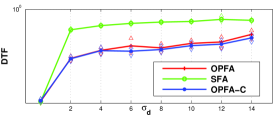
Figure 6: MSE (top) and DTF (bottom) as a function of delay variance $\sigma_{d}^{2}$ for OPFA and Sparse Factor Analysis (SFA). These curves are plotted with 95% confidence intervals. For $\sigma_{d}^{2}>0$, OPFA outperforms SFA both in MSE and DTF, maintaining its advantage as $\sigma_{d}$ increases. For large $\sigma_{d}$, OPFA-C outperforms the other two.

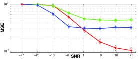
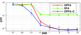
Figure 7: Same as Figure 6 except that the performance curves are plotted with respect to SNR for fixed $\sigma_{d}^{2}=5$.

IV-B Experimental data: Predictive Health and Disease (PHD)

The PHD data set was collected as part of a viral challenge study that is described in [11]. In this study 20 human subjects were inoculated with live H3N2 virus and Genechip mRNA gene expression in peripheral blood of each subject was measured over 16 time points. The raw Genechip array data was pre-processed using robust multi-array analysis [22] with quantile normalization [33]. In this section we show results for the constrained OPFA model (OPFA-C). While not shown here, we have observed that OPFA-C gives very similar results to unconstrained OPFA but with reduced computation time.

Specifically, we use OPFA-C to perform the following tasks:

1. Subject Alignment: Determine the alignment of the factors to fit each subject’s response, therefore revealing each subject’s intrinsic response delays.

2. Gene Clustering: Discover groups of genes with common expression signature by clustering in the low-dimensional space spanned by the aligned factors. Since we are using the OPFA-C model, the projection of each subject’s data on this lower dimensional space is given by the scores $\bm{A}:=\bm{A}_{1}=\cdots=\bm{A}_{S}$. Genes with similar scores will have similar expression signatures.

3. Symptomatic Gene Signature discovery: Using the gene clusters obtained in step 2 we construct temporal signatures common to subjects who became sick.

The data was normalized by dividing each element of each data matrix by the sum of the elements in its column. Since the data is non-negative valued, this will ensure that the mixing weights of different subjects are within the same order of magnitude, which is necessary to respect the assumption that $\bm{A}_{1}=\cdots=\bm{A}_{S}$ in OPFA-C. In order to select a subset of strongly varying genes, we applied one-way Analysis-Of-Variance [34] to test for the equality of the mean of each gene at 4 different groups of time points, and selected the first $p=300$ genes ranked according to the resulting F-statistic. To these gene trajectories we applied OPFA-C to the $S=9$ symptomatic subjects in the study. In this context, the columns in $\bm{F}$ are the set of signals emitted by the common immune system response and the vector $\bm{d}^{s}$ parameterizes each subject’s characteristic onset times for the factors contained in the columns of $\bm{F}$. To avoid wrap-around effects, we worked with a factor model of dimension $n=24$ in the temporal axis.

The OPFA-C algorithm was run with 4 random initializations and retained the solution yielding the minimum of the objective function (6). For each $f=1,\cdots,5$ (number of factors), we estimated the tuning parameters $(\lambda,\beta)$ following the Cross-Validation approach described in III-C over a $10\times 3$ grid. The resulting results, shown in Table IV resulted in selecting $\beta=1\times 10^{-8}$, $\lambda=1\times 10^{-8}$ and $f=3$. The choice of three factors is also consistent with an expectation that the principal gene trajectories over the period of time studied are a linear combination of increasing, decreasing or constant expression patterns [11].

TABLE IV: Cross Validation Results for Section IV-B.

	$f=1$	$f=2$	$\mathbf{f=3}$	$f=4$	$f=5$
$\min\mbox{CV}\left(f,\lambda,\beta\right)$	20.25	13.66	12.66	12.75	12.72
Relative residual	7.2	4.8	4.5	4.5	4.4
error ($\times 10^{-3}$)
$\hat{\lambda}$($\times 10^{-8}$)	5.99	1	1	1	35.9
$\hat{\beta}$ ($\times 10^{-6}$)	3.16	3.16	0.01	0.01	100

To illustrate the goodness-of-fit of our model, we plot in Figure 8 the observed gene expression patterns of 13 strongly varying genes and compare them to the OPFA-C fitted response for three of the subjects, together with the relative residual error. The average relative residual error is below $10\%$ and the plots demonstrate the agreement between the observed and the fitted patterns. Figure 9 shows the trajectories for each subject for four genes having different regulation motifs: up-regulation and down-regulation. It is clear that the gene trajectories have been smoothed while conserving their temporal pattern and their precedence-order, e.g. the up-regulation of gene OAS1 consistently follows the down-regulation of gene ORM1.

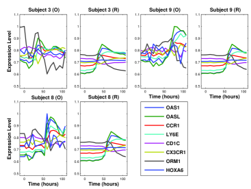
Figure 8: Comparison of observed (O) and fitted responses (R) for three of the subjects and a subset of genes in the PHD data set. Gene expression profiles for all subjects were reconstructed with a relative residual error below 10%. The trajectories are smoothed while respecting each subject’s intrinsic delay.

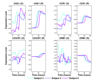
Figure 9: Comparison of observed (O) and fitted responses (R) for four genes (OAS1, CCR1, CX3CR1, ORM1) showing up-regulation and down-regulation motifs and three subjects in the PHD dataset. The gene trajectories have been smoothed while conserving their temporal pattern and their precedence-order. The OPFA-C model revealed that OAS1 up-regulation occurs consistently after ORM1 down-regulation among all subjects.

In Figure 10 we show the 3 factors along with the factor delays and factor loading discovered by OPFA-C. The three factors, shown in the three bottom panels of the figure, exhibit features of three different motifs: factor 1 and factor 3 correspond to up-regulation motifs occurring at different times; and factor 2 is a strong down-regulation motif. The three top panels show the onset times of each motif as compared to the clinically determined peak symptom onset time. Note, for example, that the strong up-regulation pattern of the first factor coincides closely with the onset peak time. Genes strongly associated to this factor have been closely associated to acute anti-viral and inflammatory host response [11]. Interestingly, the down-regulation motifs associated with factor 2 consistently precedes this up-regulation motif.

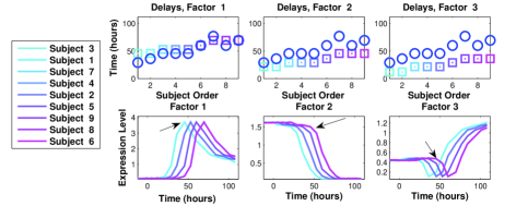
Figure 10: Top plots: Motif onset time for each factor (□) and peak symptom time reported by expert clinicians (O). Bottom plots: Aligned factors for each subject. Factor 1 and 3 can be interpreted as up-regulation motifs and factor 2 is a strong down-regulation pattern. The arrows show each factor’s motif onset time.

Finally, we consider the application of OPFA as a pre-processing step preceding a clustering analysis. Here the goal is to find groups of genes that share similar expression patterns and determine their characteristic expression patterns. In order to obtain gene clusters, we perform hierarchical clustering on the raw data ($\left\{\bm{X}_{s}\right\}_{s=1}^{S}$) and on the lower dimensional space of the estimated factor scores ( $\{\bm{A}_{s}\}_{s=1}^{S}$), obtaining two different sets of 4 well-differentiated clusters. We then compute the average expression signatures of the genes in each cluster by averaging over the observed data ($\left\{\bm{X}_{s}\right\}_{s=1}^{S}$) and averaging over the data after OPFA correction for the temporal misalignments. Figure 11 illustrates the results. Clustering using the OPFA-C factor scores produces a very significant improvement in cluster concentration as compared to clustering using the raw data $\left\{\bm{X}_{s}\right\}_{s=1}^{S}$. The first two columns in Figure compare the variation of the gene profiles over each cluster for the temporally realigned data (labeled `A´) as compared to to the profile variation of these same genes for the misaligned observed data (labeled `M´). For comparison, the last column shows the results of applying hierarchical clustering directly to the original misaligned dataset $\left\{\bm{X}_{s}\right\}_{s=1}^{S}$. It is clear that clustering on the low-dimensional space of the OPFA-C scores unveils interesting motifs from the original noisy temporal expression trajectories.

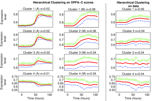
Figure 11: The first two columns show the average expression signatures and their estimated upper/lower confidence intervals for each cluster of genes obtained by: averaging the estimated Aligned expression patterns over the $S=9$ subjects (A) and directly averaging the misaligned observed data for each of the gene clusters obtained from the OPFA-C scores (M). The confidence intervals are computed according to $+/-$ the estimated standard deviation at each time point. The cluster average standard deviation ($\sigma$) is computed as the average of the standard deviations at each time point. The last column shows the results of applying hierarchical clustering directly to the original misaligned dataset $\left\{\bm{X}_{s}\right\}_{s=1}^{S}$. In the first column, each gene expression pattern is obtained by mixing the estimated aligned factors $\bm{F}$ according to the estimated scores $\bm{A}$. The alignment effect is clear, and interesting motifs become more evident.

V Conclusions

We have proposed a general method of order-preserving factor analysis that accounts for possible temporal misalignments in a population of subjects undergoing a common treatment. We have described a simple model based on circular-shift translations of prototype motifs and have shown how to embed transient gene expression time courses into this periodic model. The OPFA model can significantly improve interpretability of complex misaligned data. The method is applicable to other signal processing areas beyond gene expression time course analysis.

A Matlab package implementing OPFA and OPFA-C will be available at the Hero Group Reproducible Research page (http://tbayes.eecs.umich.edu).

-A Circulant time shift model

Using circular shifts in (3) introduces periodicity into our model (2). Some types of gene expression may display periodicity, e.g. circadian transcripts, while others, e.g. transient host response, may not. For transient gene expression profiles such as the ones we are interested in here, we use a truncated version of this periodic model, where we assume that each subject’s response arises from the observation of a longer periodic vector within a time window (see Figure 12):

$$\bm{X}_{s}=\left[\bm{M}\left(\bm{F},\bm{d}^{s}\right)\bm{A}_{s}+\bm{\epsilon}_{s}\right]_{\Omega}.$$ (32)

Here, the factors are of dimension $n_{F}\geq n$ and the window size is of dimension $n$ (in the special case that $n=n_{F}$, we have the original periodic model). In this model, the observed features are non-periodic as long as the delays $\bm{d}^{s}$ are sufficiently small as compared to $n_{F}$. More concretely, if the maximum delay is $d_{\max}$, then in order to avoid wrap-around effects the dimension should be chosen as at least $n_{F}=n+d_{\max}$. Finally, we define the index set $\Omega$ corresponding to the observation window as:

$$\Omega=\left\{\omega^{1},\omega^{1}+1,\omega^{1}+2...,\omega^{2}\right\}^{p}$$ (33)

where $\omega^{1}$ and $\omega^{2}$ are the lower and upper observation endpoints, verifying $n=\omega^{2}-\omega^{1}$.

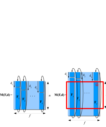
Figure 12: Right: Each subject’s factor matrix $\bm{M}_{i}$ is obtained by applying a circular shift to a common set of factors $\bm{F}$ parameterized by a vector $\bm{d}$. Left: In order to avoid wrap-around effects when modeling transient responses, we consider instead a higher dimensional truncated model of dimension $n_{F}$ from which we only observe the elements within the window characterized by $\Omega$.

-B Delay estimation and time-course alignment

The solution to problem (9) yields an estimate $\hat{\bm{d}}^{s}$ for each subject’s intrinsic factor delays. These delays are relative to the patterns found in the estimated factors and therefore require conversion to a common reference time.

For a given up-regulation or down-regulation motif, $I$, which we call the feature of interest, found in factor $g$, we choose a time point of interest $t_{I}$. See Figure 13 (a) for an example of choice of $t_{I}$ for an up-regulation feature.

Then, given $t_{I}$ and for each subject $s$ and each factor $k$, we define the absolute feature occurrence time as follows:

$$t_{s,k}=\left(\hat{\bm{d}}^{s}_{k}+t_{I}\right)\mbox{mod}~{}n_{F}-\omega^{1}.$$ (34)

where $\hat{\bm{d}}^{s}_{g}$ is the estimated delay corresponding to factor $k$ and subject $s$ and $\omega^{1}$ is the lower endpoint of the observation window (see (33)). Figure 13 illustrates the computation of $t_{s,k}$ in a 2-factor example.

The quantities $t_{s,k}$ can be used for interpretation purposes or to realign temporal profiles in order to find common, low-variance gene expression signatures, as shown in Section IV-B.

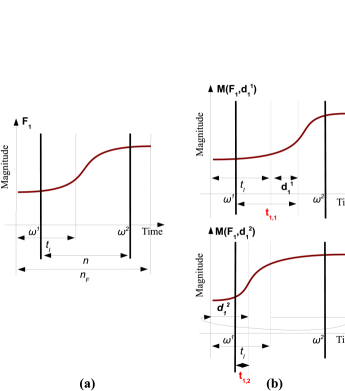
Figure 13: (a) Time point of interest ($t_{I}$) for the up-regulation feature of factor 1. (b) The absolute time points $t_{1,1}$, $t_{1,2}$ are shown in red font for two different subjects and have been computed according to their corresponding relative delays and the formula in (34).

-C Implementation of EstimateFactors and EstimateScores

We consider here the implementation of EstimateFactors and EstimateScores under the presence of missing data. Let $\Omega_{s}=\left[\omega^{s}_{1},\cdots,\omega^{s}_{p}\right]\in\left\{0,1\right\}^{n\times p}$ be the set of observed entries in observation $\bm{X}_{s}$. The objective in (9) is then:

$$\sum_{s=1}^{S}\left|\left|\left[\bm{X}_{s}-\bm{M}\left({\bm{F}},{\bm{d}}^{s}\right){\bm{A}}_{s}\right]_{\Omega_{s}}\right|\right|_{F}^{2}$$ (35)

We will show how to reformulate problems EstimateFactors (14) and EstimateScores (18) in a standard quadratic objective with linear and/or quadratic constraints.

First, we rewrite the objective (35) as:

$$\sum_{s=1}^{S}\sum_{j=1}^{p}\left|\left|\mbox{diag}\left(\omega^{s}_{j}\right)\left[\bm{X}_{s}\right]_{\cdot,j}-\mbox{diag}\left(\omega^{s}_{j}\right)\bm{M}\left(\bm{F},\bm{d}^{s}\right)\left[\bm{A}_{s}\right]_{\cdot,j}\right|\right|_{F}^{2}.$$

Expanding the square we obtain:

$$\sum_{s=1}^{S}\left|\left|\left[\bm{X}_{s}-\bm{M}\left(\bm{F},\bm{d}^{s}\right)\bm{A}_{s}\right]_{\Omega_{s}}\right|\right|_{F}^{2} =\sum_{s=1}^{S}\sum_{j=1}^{p}\left[\bm{A}_{s}\right]_{\cdot,j}^{T}\bm{M}\left(\bm{F},\bm{d}^{s}\right)^{T}\mbox{diag}\left(\omega^{s}_{j}\right)\bm{M}\left(\bm{F},\bm{d}^{s}\right)\left[\bm{A}_{s}\right]_{\cdot,j}$$ (36)

$$-2\left[\bm{X}_{s}\right]_{\cdot,j}^{T}\mbox{diag}\left(\omega^{s}_{j}\right)\bm{M}\left(\bm{F},\bm{d}^{s}\right)\left[\bm{A}_{s}\right]_{\cdot,j}$$

$$+\sum_{s=1}^{S}\left|\left|\left[\bm{X}_{s}\right]_{\Omega_{s}}\right|\right|_{F}^{2}.$$

To obtain the EstimateFactors objective, first we will rewrite the OPFA model (32) using matrix notation. Let $\bm{U}_{i}$ be a circular shift matrix $\bm{U}_{i}$ parameterized by the $i$-th delay $\bm{d}$ component. Then

$$\bm{M}\left(\bm{F},\bm{d}\right)=\left[\bm{U}_{1}\bm{F}_{1},\cdots,\bm{U}_{f}\bm{F}_{f}\right]=\bm{H}\tilde{\bm{F}}$$

where $\bm{F}_{j}$ denotes the $j$-th column of $\bm{F}$, $\bm{H}$ is the concatenation of the $\bm{U}_{i}$ matrices and $\tilde{\bm{F}}$ is a matrix containing the columns of $\bm{F}$ with the appropriate padding of zeros. With this notation and (36) we obtain:

$$\sum_{s=1}^{S}\left|\left|\left[\bm{X}_{s}-\bm{M}\left(\bm{F},\bm{d}^{s}\right)\bm{A}_{s}\right]_{\Omega_{s}}\right|\right|_{F}^{2} \propto_{\bm{F}}\sum_{s=1}^{S}\sum_{j=1}^{p}\mbox{tr}\left(\left[\bm{A}_{s}\right]_{\cdot,j}\left[\bm{A}_{s}\right]_{\cdot,j}^{T}\tilde{\bm{F}}^{T}\bm{H}_{s}^{T}\mbox{diag}\left(\omega^{s}_{j}\right)\bm{H}_{s}\tilde{\bm{F}}\right)$$

$$-2\mbox{tr}\left(\left[\bm{A}_{s}\right]_{\cdot,j}\left[\bm{X}_{s}\right]_{\cdot,j}^{T}\mbox{diag}\left(\omega^{s}_{j}\right)\bm{H}_{s}\tilde{\bm{F}}\right).$$

We now use the identity ([35], Thm. 3 Sec. 4):

$$\mbox{tr}\left(\bm{Z}\bm{X}^{T}\bm{Y}\bm{W}\right)=\mbox{vec}\left(\bm{W}\right)^{T}\bm{Z}\otimes\bm{Y}^{T}\mbox{vec}\left(\bm{X}\right),$$

to write:

$$\sum_{s=1}^{S}\left|\left|\left[\bm{X}_{s}-\bm{M}\left(\bm{F},\bm{d}^{s}\right)\bm{A}_{s}\right]_{\Omega_{s}}\right|\right|_{F}^{2} \propto_{\bm{F}}\mbox{vec}\left(\tilde{\bm{F}}\right)^{T}\left(\sum_{s=1}^{S}\sum_{j=1}^{p}\left[\bm{A}_{s}\right]_{\cdot,j}\left[\bm{A}_{s}\right]_{\cdot,j}^{T}\otimes\bm{H}_{s}^{T}\mbox{diag}\left(\omega^{s}_{j}\right)\bm{H}_{s}\right)\mbox{vec}\left(\tilde{\bm{F}}\right)$$

$$-2\mbox{vec}\left(\sum_{s=1}^{S}\sum_{j=1}^{p}\bm{H}_{s}^{T}\mbox{diag}\left(\omega^{s}_{j}\right)\left[\bm{X}_{s}\right]_{\cdot,j}\left[\bm{A}_{s}\right]_{\cdot,j}^{T}\right)\mbox{vec}\left(\tilde{\bm{F}}\right).$$

Finally, making use of the fact that $\tilde{\bm{F}}$ is a block-column matrix with the columns of $\bm{F}$ padded by zeros, we conclude:

$$\sum_{s=1}^{S}\left|\left|\left[\bm{X}_{s}-\bm{M}\left(\bm{F},\bm{d}^{s}\right)\bm{A}_{s}\right]_{\Omega_{s}}\right|\right|_{F}^{2} \propto_{\bm{F}}\mbox{vec}\left(\bm{F}\right)^{T}\bm{Q}_{F}\mbox{vec}\left({\bm{F}}\right)-2\bm{q}_{F}^{T}\mbox{vec}\left({\bm{F}}\right)$$

where we have defined

$$\bm{Q}_{F}=\left[\sum_{s=1}^{S}\sum_{j=1}^{p}\left[\bm{A}_{s}\right]_{\cdot,j}\left[\bm{A}_{s}\right]_{\cdot,j}^{T}\otimes\bm{H}_{s}^{T}\mbox{diag}\left(\omega^{s}_{j}\right)\bm{H}_{s}\right]_{\mathcal{J},\mathcal{J}}$$ (37)

$$\bm{q}_{F}=\left[\mbox{vec}\left(\sum_{s=1}^{S}\sum_{j=1}^{p}\bm{H}_{s}^{T}\mbox{diag}\left(\omega^{s}_{j}\right)\left[\bm{X}_{s}\right]_{\cdot,j}\left[\bm{A}_{s}\right]_{\cdot,j}^{T}\right)\right]_{\mathcal{J}}$$ (38)

and $\mathcal{J}$ are the indices corresponding to the non-zero elements in $\mbox{vec}\left(\tilde{\bm{F}}\right)$. Hence, EstimateFactors can be written as:

$$\min_{\bm{F}} \mbox{vec}\left(\bm{F}\right)^{T}\left(\bm{Q}_{F}+\beta\mbox{diag}\left(\bm{W}^{T}\bm{W},\cdots,\bm{W}^{T}\bm{W}\right)\right)\mbox{vec}\left({\bm{F}}\right)-2\bm{q}_{F}^{T}\mbox{vec}\left({\bm{F}}\right)$$

s.t. $$\left\{\begin{array}[]{c c}\left|\left|\bm{F}\right|\right|^{2}_{\mathcal{F}}\leq\delta&\\ \bm{F}_{i,j}\geq 0&i=1,\cdots,n,\\ &j=1,\cdots,f\end{array}\right.$$

The dimension of the variables in this problem is $nf$. In the applications considered here, both $n$ and $f$ are relatively small and hence this program can be solved with a standard convex solver such as SeDuMi [36] (upon conversion to a standard conic problem).

On the other hand, we can follow the same procedure to reformulate the objective in EstimateScores (18) into a penalized quadratic form. First we use (36) and (-C) to write:

$$\sum_{s=1}^{S}\left|\left|\left[\bm{X}_{s}-\bm{M}\left(\bm{F},\bm{d}^{s}\right)\bm{A}_{s}\right]_{\Omega_{s}}\right|\right|_{F}^{2} \propto_{\left\{\bm{A}_{s}\right\}_{i=1}^{S}}\sum_{s=1}^{S}\mbox{vec}\left(\bm{A}_{s}\right)^{T}\bm{Q}^{s}_{A}\mbox{vec}\left(\bm{A}_{s}\right)-2{\bm{q}^{s}_{A}}^{T}\mbox{vec}\left(\bm{A}_{s}\right)$$

where

$$\bm{Q}^{s}_{A}=\left[\begin{array}[]{cccc}\bm{M}\left(\bm{F},\bm{d}^{s}\right)^{T}\mbox{diag}\left(\omega^{s}_{1}\right)\bm{M}\left(\bm{F},\bm{d}^{s}\right)&\bm{0}&\dots&\bm{0}\\ \bm{0}&\bm{0}&\cdots&\bm{0}\\ \bm{0}&\cdots&\bm{0}&\bm{M}\left(\bm{F},\bm{d}^{s}\right)^{T}\mbox{diag}\left(\omega^{s}_{p}\right)\bm{M}\left(\bm{F},\bm{d}^{s}\right)\end{array}\right]$$ (43)

$$\bm{q}^{s}_{A}=\left[\begin{array}[]{ccc}\left[\bm{X}_{s}\right]_{\cdot,1}^{T}\mbox{diag}\left(\omega^{s}_{1}\right)\bm{M}\left(\bm{F},\bm{d}^{s}\right)&\cdots&\left[\bm{X}_{s}\right]_{\cdot,p}^{T}\mbox{diag}\left(\omega^{s}_{p}\right)\bm{M}\left(\bm{F},\bm{d}^{s}\right)\end{array}\right].$$ (45)

Thus EstimateFactors can be written as:

$$\min_{\bm{F}} \sum_{s=1}^{S}\mbox{vec}\left(\bm{A}_{s}\right)^{T}\bm{Q}^{s}_{A}\mbox{vec}\left(\bm{A}_{s}\right)-2{\bm{q}^{s}_{A}}^{T}\mbox{vec}\left(\bm{A}_{s}\right)+\lambda\sum_{i=1}^{p}\sum_{j=1}^{f}\|\left[\bm{A}_{1}\right]_{j,i}\cdots\left[\bm{A}_{S}\right]_{j,i}\|_{2}$$ (46)

s.t. $$\left\{\begin{array}[]{c c}\left|\left|\bm{F}\right|\right|^{2}_{\mathcal{F}}\leq\delta&\\ \bm{F}_{i,j}\geq 0&i=1,\cdots,n,\\ &j=1,\cdots,f\end{array}\right.$$ (49)

This is a convex, non-differentiable and potentially high-dimensional problem. For this type of optimization problems, there exists a class of simple and scalable algorithms which has recently received much attention [37], [38], [39], [28]. These algorithms rely only on first-order updates of the type:

$$\bm{\bm{x}}^{t}\leftarrow\mathcal{T}_{\Gamma,\lambda}\left(\bm{v}-2\bm{\bm{x}}^{t-1}\left(\alpha\bm{I}-\bm{Q}\right)\right),$$ (50)

which only involves matrix-vector multiplications and evaluation of the operator $\mathcal{T}$, which is called the proximal operator [39] associated to $\Gamma$ and $\mathcal{C}$ and is defined as:

$$\mathcal{T}_{\Gamma,\lambda}\left(\bm{v}\right) :=\min \frac{1}{2}\bm{x}^{\prime}\bm{x}+\bm{v}^{\prime}\bm{x}+\lambda\Gamma\left(\bm{x}\right)$$

s.t. $$\bm{x}\in\mathcal{C}.$$

This operator takes the vector $\bm{v}$ as an input and outputs a shrunk/thresholded version of it depending on the nature of the penalty $\Gamma$ and the constraint set $\mathcal{C}$. For some classes of penalties $\Gamma$ (e.g. $l_{1}$, $l_{2}$, mixed $l_{1}-l_{2}$) and the positivity constraints considered here, this operator has a closed form solution [40], [39]. Weak convergence of the sequence (50) to the optimum of (46) is assured for a suitable choice of the constant $\alpha$ [28], [41].

-D Delay Estimation lower bound in the presence of Missing Data

As we mentioned earlier, the lower bound (29) does not hold anymore under the presence of missing data. We derive here another bound that can be used in such case. From expression (36), we first obtain the objective in EstimateDelays (23) in a quadratic form:

$$\sum_{s=1}^{S}\left|\left|\left[\bm{X}_{s}-\bm{M}\left(\bm{F},\bm{d}^{s}\right)\bm{A}_{s}\right]_{\Omega_{s}}\right|\right|_{F}^{2} \propto_{\bm{d}^{s}}\sum_{s=1}^{S}\sum_{j=1}^{p}\mbox{tr}\left(\bm{M}\left(\bm{F},\bm{d}^{s}\right)^{T}\mbox{diag}\left(\omega^{s}_{j}\right)\bm{M}\left(\bm{F},\bm{d}^{s}\right)\bm{P}_{s,j}\right)$$

$$-2\mbox{tr}\left(\bm{Q}_{s,j}\bm{M}\left(\bm{F},\bm{d}^{s}\right)\right).$$

Where we have let $\bm{P}_{s,j}:=\left[\bm{A}_{s}\right]_{\cdot,j}\left[\bm{A}_{s}\right]_{\cdot,j}^{T}$ and $\bm{Q}_{s,j}=\left[\bm{A}_{s}\right]_{\cdot,j}\left[\bm{X}_{s}\right]_{\cdot,j}^{T}\mbox{diag}\left(\omega^{s}_{j}\right)$. Notice that each of the terms indexed by $s$ is independent of the others. Using (-C), we obtain

$$\left|\left|\left[\bm{X}_{s}-\bm{M}\left(\bm{F},\bm{d}^{s}\right)\bm{A}_{s}\right]_{\Omega_{s}}\right|\right|_{F}^{2} \propto\mbox{vec}\left(\bm{M}\left(\bm{F},\bm{d}^{s}\right)\right)^{T}\sum_{j=1}^{p}\left(\bm{P}_{s,j}\otimes\mbox{diag}\left(\omega^{s}_{j}\right)\right)\mbox{vec}\left(\bm{M}\left(\bm{F},\bm{d}^{s}\right)\right)$$

$$-2\mbox{vec}\left(\sum_{j=1}^{p}\bm{Q}_{s,j}^{T}\right)^{T}\mbox{vec}\left(\bm{M}\left(\bm{F},\bm{d}^{s}\right)\right).$$

We now can minorize the function above by:

$$\left|\left|\left[\bm{X}_{s}-\bm{M}\left(\bm{F},\bm{d}^{s}\right)\bm{A}_{s}\right]_{\Omega_{s}}\right|\right|_{F}^{2} \geq\underline{\lambda}\left(\sum_{j=1}^{p}\bm{P}_{s,j}\otimes\mbox{diag}\left(\omega^{s}_{j}\right)\right)\mbox{vec}\left(\bm{M}\left(\bm{F},\bm{d}^{s}\right)\right)^{T}\mbox{vec}\left(\bm{M}\left(\bm{F},\bm{d}^{s}\right)\right)$$

$$-2\mbox{vec}\left(\sum_{j=1}^{p}\bm{Q}_{s,j}^{T}\right)^{T}\mbox{vec}\left(\bm{M}\left(\bm{F},\bm{d}^{s}\right)\right)+\sum_{s=1}^{S}\left|\left|\left[\bm{X}_{s}\right]_{\Omega_{s}}\right|\right|_{F}^{2}$$

which leads to:

$$\left|\left|\left[\bm{X}_{s}-\bm{M}\left(\bm{F},\bm{d}^{s}\right)\bm{A}_{s}\right]_{\Omega_{s}}\right|\right|_{F}^{2} \geq\underline{\lambda}\left(\sum_{j=1}^{p}\bm{P}_{s,j}\otimes\mbox{diag}\left(\omega^{s}_{j}\right)\right)\left|\left|\bm{F}\right|\right|_{F}^{2}$$

$$-2\mbox{vec}\left(\sum_{j=1}^{p}\bm{Q}_{s,j}^{T}\right)^{T}\mbox{vec}\left(\bm{M}\left(\bm{F},\bm{d}^{s}\right)\right)+\left|\left|\left[\bm{X}_{s}\right]_{\Omega_{s}}\right|\right|_{F}^{2}.$$

Using the relaxation in (27), we can now compute a lower bound $\Phi_{lb}\left({\mathcal{I}}_{t}\right)$ as

$$\Phi_{lb}\left({\mathcal{I}}_{t}\right) =\underline{\lambda}\left(\sum_{j=1}^{p}\bm{P}_{s,j}\otimes\mbox{diag}\left(\omega^{s}_{j}\right)\right)\left|\left|\bm{F}\right|\right|_{F}^{2}+\left|\left|\left[\bm{X}_{s}\right]_{\Omega_{s}}\right|\right|_{F}^{2}$$

$$-2\max_{\bm{d}\in{\mathcal{S}}_{t}}\mbox{vec}\left(\sum_{j=1}^{p}\bm{Q}_{s,j}^{T}\right)^{T}\mbox{vec}\left(\bm{M}\left(\bm{F},\bm{d}^{s}\right)\right).$$

References

- [1] I. Johnstone and A. Lu, “On consistency and sparsity for principal components analysis in high dimensions,” Journal of the American Statistical Association, vol. 104, no. 486, pp. 682–693, 2009.
- [2] R. Jenatton, G. Obozinski, and F. Bach, “Structured Sparse Principal Component Analysis,” in Proceedings of the 13th International Conference on Artificial Intelligence and Statistics (AISTATS) 2010, vol. 9, 2010.
- [3] T. Blumensath and M. Davies, “Sparse and shift-invariant representations of music,” IEEE Transactions on Speech and Audio Processing, vol. 14, no. 1, p. 50, 2006.
- [4] K. Pearson, “LIII. On lines and planes of closest fit to systems of points in space,” Philosophical Magazine Series 6, vol. 2, no. 11, pp. 559–572, 1901.
- [5] J. Carroll and J. Chang, “Analysis of individual differences in multidimensional scaling via an N-way generalization of Eckart-Young decomposition,” Psychometrika, vol. 35, no. 3, pp. 283–319, 1970.
- [6] M. Aharon, M. Elad, and A. Bruckstein, “K-SVD: An algorithm for designing overcomplete dictionaries for sparse representation,” IEEE Transactions on signal processing, vol. 54, no. 11, pp. 4311–4322, 2006.
- [7] K. Kreutz-Delgado, J. Murray, B. Rao, K. Engan, T. Lee, and T. Sejnowski, “Dictionary learning algorithms for sparse representation,” Neural computation, vol. 15, no. 2, pp. 349–396, 2003.
- [8] B. Olshausen and D. Field, “Sparse coding with an overcomplete basis set: A strategy employed by V1?” Vision research, vol. 37, no. 23, pp. 3311–3325, 1997.
- [9] D. Witten, R. Tibshirani, and T. Hastie, “A penalized matrix decomposition, with applications to sparse principal components and canonical correlation analysis,” Biostatistics, vol. 10, no. 3, p. 515, 2009.
- [10] B. Mailhé, S. Lesage, R. Gribonval, F. Bimbot, and P. Vandergheynst, “Shift-invariant dictionary learning for sparse representations: extending K-SVD,” in Proceedings of the 16th European Signal Processing Conference, vol. 4, 2008.
- [11] A. Zaas, M. Chen, J. Varkey, T. Veldman, A. Hero, J. Lucas, Y. Huang, R. Turner, A. Gilbert, R. Lambkin-Williams et al., “Gene Expression Signatures Diagnose Influenza and Other Symptomatic Respiratory Viral Infections in Humans,” Cell Host & Microbe, vol. 6, no. 3, pp. 207–217, 2009.
- [12] N. Sidiropoulos, G. Giannakis, and R. Bro, “Blind PARAFAC receivers for DS-CDMA systems,” IEEE Transactions on Signal Processing, vol. 48, no. 3, pp. 810–823, 2000.
- [13] D. Lee and H. Seung, “Learning the parts of objects by non-negative matrix factorization,” Nature, vol. 401, no. 6755, pp. 788–791, 1999.
- [14] N. Srebro, J. Rennie, and T. Jaakkola, “Maximum-margin matrix factorization,” Advances in neural information processing systems, vol. 17, pp. 1329–1336, 2005.
- [15] T. Kolda and B. Bader, “Tensor decompositions and applications,” SIAM Review, vol. 51, no. 3, pp. 455–500, 2009.
- [16] G. Bergqvist and E. Larsson, “The higher-order singular value decomposition: Theory and an application [lecture notes],” Signal Processing Magazine, IEEE, vol. 27, no. 3, pp. 151 –154, 2010.
- [17] A. d’Aspremont, L. El Ghaoui, M. Jordan, and G. Lanckriet, “A Direct Formulation for Sparse PCA Using Semidefinite Programming,” SIAM Review, vol. 49, no. 3, pp. 434–448, 2007.
- [18] M. Lewicki and T. Sejnowski, “Coding time-varying signals using sparse, shift-invariant representations,” Advances in neural information processing systems, pp. 730–736, 1999.
- [19] A. Tibau Puig, A. Wiesel, and A. Hero, “Order-preserving factor analysis,” University of Michigan, Tech. Rep., June 2010.
- [20] L. Sacchi, C. Larizza, P. Magni, and R. Bellazzi, “Precedence Temporal Networks to represent temporal relationships in gene expression data,” Journal of Biomedical Informatics, vol. 40, no. 6, pp. 761–774, 2007.
- [21] A. Aderem and R. Ulevitch, “Toll-like receptors in the induction of the innate immune response,” Nature, vol. 406, no. 6797, pp. 782–787, 2000.
- [22] R. Irizarry, B. Hobbs, F. Collin, Y. Beazer-Barclay, K. Antonellis, U. Scherf, and T. Speed, “Exploration, normalization, and summaries of high density oligonucleotide array probe level data,” Biostatistics, vol. 4, no. 2, p. 249, 2003.
- [23] P. Comon, Tensor decompositions, ser. Mathematics in signal processing V. Oxford University Press, USA, 2002.
- [24] L. De Lathauwer, B. De Moor, and J. Vandewalle, “A multilinear singular value decomposition,” SIAM Journal on Matrix Analysis and Applications, vol. 21, no. 4, pp. 1253–1278, 2000.
- [25] Y. Jia, M. Salzmann, and T. Darrell, “Factorized latent spaces with structured sparsity,” EECS Department, University of California, Berkeley, Tech. Rep. UCB/EECS-2010-99, Jun 2010.
- [26] J. Mairal, F. Bach, J. Ponce, G. Sapiro, and A. Zisserman, “Non-local sparse models for image restoration,” in Computer Vision, 2009 IEEE 12th International Conference on. IEEE, 2010, pp. 2272–2279.
- [27] M. Yuan and Y. Lin, “Model selection and estimation in regression with grouped variables,” Journal of the Royal Statistical Society Series B Statistical Methodology, vol. 68, no. 1, p. 49, 2006.
- [28] N. Pustelnik, C. Chaux, and J. Pesquet, “A constrained forward-backward algorithm for image recovery problems,” in Proceedings of the 16th European Signal Processing Conference, 2008, pp. 25–29.
- [29] E. Lawler and D. Wood, “Branch-and-bound methods: A survey,” Operations research, vol. 14, no. 4, pp. 699–719, 1966.
- [30] A. Owen and P. Perry, “Bi-cross-validation of the SVD and the nonnegative matrix factorization,” The Annals of Applied Statistics, vol. 3, no. 2, pp. 564–594, 2009.
- [31] S. Wold, “Cross-validatory estimation of the number of components in factor and principal components models,” Technometrics, vol. 20, no. 4, pp. 397–405, 1978.
- [32] T. Hastie, R. Tibshirani, and J. Friedman, The elements of statistical learning: data mining, inference and prediction. Springer, 2005.
- [33] B. Bolstad, R. Irizarry, M. Astrand, and T. Speed, “A comparison of normalization methods for high density oligonucleotide array data based on variance and bias,” Bioinformatics, vol. 19, no. 2, p. 185, 2003.
- [34] J. Neter, W. Wasserman, M. Kutner et al., Applied linear statistical models. Irwin Burr Ridge, Illinois, 1996.
- [35] H. Neudecker and J. Magnus, “Matrix Differential Calculus with Applications in Statistics and Econometrics,” 1999.
- [36] J. Sturm, “Using SeDuMi 1.02, a MATLAB toolbox for optimization over symmetric cones,” Optimization methods and software, vol. 11, no. 1, pp. 625–653, 1999.
- [37] M. Zibulevsky and M. Elad, “L1-l2 optimization in signal and image processing,” Signal Processing Magazine, IEEE, vol. 27, no. 3, pp. 76 –88, may 2010.
- [38] I. Daubechies, M. Defrise, and C. De Mol, “An iterative thresholding algorithm for linear inverse problems with a sparsity constraint,” Communications on Pure and Applied Mathematics, vol. 57, no. 11, pp. 1413–1457, 2004.
- [39] P. Combettes and V. Wajs, “Signal recovery by proximal forward-backward splitting,” Multiscale Modeling and Simulation, vol. 4, no. 4, pp. 1168–1200, 2006.
- [40] A. Tibau Puig, A. Wiesel, and A. O. Hero, “A multidimensional shrinkage-thresholding operator,” in Statistical Signal Processing, 2009. SSP ’09. IEEE/SP 15th Workshop on, 2009, pp. 113 – 116.
- [41] A. Beck and M. Teboulle, “A fast iterative shrinkage-thresholding algorithm for linear inverse problems,” SIAM J. Imaging Sci, vol. 2, pp. 183–202, 2009.