Single-lined Spectroscopic Binary Star Candidates in the RAVE Survey

Abstract

Repeated spectroscopic observations of stars in the Radial Velocity Experiment (RAVE) database are used to identify and examine single-lined binary (SB1) candidates. The RAVE latest internal database (VDR3) includes radial velocities, atmospheric and other parameters for approximately quarter million of different stars with little less than 300,000 observations. In the sample of $\sim$20,000 stars observed more than once, 1333 stars with variable radial velocities were identified. Most of them are believed to be SB1 candidates. The fraction of SB1 candidates among stars with several observations is between 10% and 15% which is the lower limit for binarity among RAVE stars. Due to the distribution of time spans between the re-observation that is biased towards relatively short timescales (days to weeks), the periods of the identified SB1 candidates are most likely in the same range. Because of the RAVE’s narrow magnitude range most of the dwarf candidates belong to the thin Galactic disk while the giants are part of the thick disk with distances extending to up to a few kpc. The comparison of the list of SB1 candidates to the VSX catalog of variable stars yielded several pulsating variables among the giant population with the radial velocity variations of up to few tens of $\mathrm{km\,s^{-1}}$. There are 26 matches between the catalog of spectroscopic binary orbits ($S_{B^{9}}$) and the whole RAVE sample for which the given periastron time and the time of RAVE observation were close enough to yield a reliable comparison. RAVE measurements of radial velocities of known spectroscopic binaries are consistent with their published radial velocity curves.

1. Introduction

Binary stars are not uncommon. Many studies searching for multiplicity among field and cluster stars of different spectral types report that the fraction of binary stars in the observed sample is as high as 50% or more for certain spectral types. Multiplicity among dwarfs and subdwarfs was studied by Duquennoy & Mayor (1991); Fischer & Marcy (1992); Lada (2006); Raghavan et al. (2010), massive binary stars by Mason et al. (2009); Sana et al. (2009) and binary stars in clusters by Abt & Willmarth (1999); Sommariva et al. (2009), and others. Same findings are also supported by numerical simulations of star cluster formation (Bate, 2009).

In the last few decades many new spectroscopic binaries were discovered, owing a large part to the successful CORAVEL and CfA speedometers and other instruments. There were several surveys dedicated to the search of spectroscopic binaries (Latham et al., 2002; Griffin, 2006; Mermilliod et al., 2007, among others). The larger scale Geneva-Copenhagen Survey (Nordström et al., 2004) aiming at the F and G type dwarfs was also successful in identification of spectroscopic binaries with a fraction of 19% in the observed sample. Many of the discovered binaries from various catalogs along with their orbital parameters are compiled by Pourbaix et al. (2004) in the $S_{B^{9}}$ catalog of spectroscopic binary orbits.

With the development of optical-fiber spectrographs that enable the observation of up to several hundred stars simultaneously, efficient large-scale spectroscopic surveys became possible. Among the largest such sky surveys with the focus on stellar objects are the Sloan Digital Sky Survey (SDSS) covering the northern sky and the Radial Velocity Experiment (RAVE; Steinmetz et al., 2006) covering the southern sky with a higher spectral resolution but narrower wavelength range than the SDSS. Binary star candidates observed as a part of the SDSS are discussed in Pourbaix et al. (2005). Double-lined spectroscopic binary (SB2) candidates discovered in the second data release of the RAVE survey where published in Matijevič et al. (2010) – Paper I hereafter. The analysis of single-lined spectroscopic binary (SB1) candidates identified in the RAVE’s latest internal database (VDR3) is the subject of this paper. Section 2 gives an overview of radial velocity (RV) acquisition in the RAVE survey. Section 3 discusses the sample of RAVE stars that were observed multiple times and the procedure that was used to identify potential SB1 objects. In Section 4, a catalog of SB1 candidates is presented. The concluding section summarizes the main results and discusses future work to use the discovered binary candidates for population analysis and to assess their influence on the Galactic RV distribution.

2. RAVE Radial Velocities

RAVE is an ongoing multi-fiber spectroscopic survey based on observations with the UK Schmidt Telescope at the Australian Astronomical Observatory (AAO) with the goal of observing up to 1 million stars in the magnitude range between $9<I<12$. The wavelength range of the spectra covers the near-infrared region $\lambda\lambda 8410-8795$ with a resolving power of $R\sim 7500$, typically with a moderately high signal-to-noise ratio (S/N; mean value of 45 pixel^-1). The RAVE spectral analysis pipeline is designed to derive accurate stellar RVs as well as atmospheric parameters and chemical composition (Boeche et al., 2010). So far, two data releases have been published (Steinmetz et al., 2006; Zwitter et al., 2008) and the third one was submitted (Siebert et al., 2011).

The measurement of stellar RVs is one of the major goals of the RAVE survey. Along with the star’s position on the sky, its proper motion and distance, an RV gives us a missing sixth kinematic component. Having full six-dimensional data for up to a million stars allows one to carry out detailed studies of structure and kinematics of the Galaxy.

All data provided by the RAVE survey are acquired at the AAO 1.2m UK Schmidt telescope with the 6dF optical fiber system feeding the dedicated spectrograph. About a hundred optical fibers are positioned in the focal plane of the telescope to route light from the same number of stars simultaneously to the slit vane mounted in the spectrograph enclosure. Additional fibers are used to observe the background sky. The slit vane stacks the endings of all fibers in a column, one over the other. Due to the close spacing of the fibers there is a chance of light cross-talk between them. Light from one fiber may be spilling into the adjacent one. This effect is minimized by observing stars in a narrow magnitude range and by data reduction pipeline which subtracts the cross-talk by an iterative procedure. Second order light which contaminates spectra from the first RAVE data release is now blocked by a blue blocking filter placed in front of the collimator. The light passing the collimator is dispersed using a volume phase holographic transmission grating and finally recorded with a camera using a CCD detector. Because the throughput of the different fibers may vary, the final $\mathrm{S/N}$ of two equally bright stars from the same field plate may be different. Typically, fields are observed in the following manner. Before and after five consecutive field exposures lasting 10 minutes each, two calibrating lamp exposures are usually made. Slight temperature variations in the spectrograph enclosure may shift the wavelength calibration so each plate has a few dedicated sky fibers that (together with sky velocities derived from stellar spectra) serve as additional wavelength constraint and are also used for the subtraction of the telluric lines present in stellar spectra (Steinmetz et al., 2006).

The measurement of RVs is performed in a following way. First, a spectrum is continuum normalized using a pair of cubic splines. Then, a four step iterative method is used to calculate its RV: (1) using a standard cross-correlation procedure (Tonry & Davis, 1979) a first RV estimate is calculated. This step requires a library of template synthetic spectra against which a correlation is calculated. A subset of 40 spectra from Munari et al. (2005) covering the whole $\{T_{\mathrm{eff}},\log g\}$ parameter space is used to get a rough estimate with a precision of $\sim 5\,\mathrm{km\ s^{-1}}$ for spectra with strong Ca II lines. (2) The spectra are shifted relative to the rest frame according to the RV estimate just calculated. (3) A best-matching template is constructed from a full library of template spectra (see Zwitter et al. (2008) for a more detailed description of this procedure). (4) With a best-matching template a new RV is calculated, and finally this measurement is corrected for a possible zero-point shift (Siebert et al., 2011) that is produced by the temperature variations in the spectrograph components. Errors of the RV measurements are estimated by fitting a parabolic curve to the peak of the cross-correlation function.

Figure 1.— Cumulative distribution of measured radial velocity errors. The dashed line represents the data from the VDR3 release with $\mathrm{S/N}>20$. The thinner black line shows a subset that includes only stars that were confidently classified as cold $(T_{\mathrm{eff}}\lesssim 7500\,\mathrm{K})$ normal single stars. The dotted line represents only the already published data from the second data release. Thicker light gray line shows the distribution of applied zero-point corrections (to correct the temperature variations, see the text) and the thicker dark gray line shows the average discrepancy between RVs and their weighted average in terms of RV errors (Equation (1)) for stars with multiple observations. Data from the first release plagued by second order light contamination are excluded in all shown sets. Dash-dotted lines mark the 50th, 68th and 95th percentiles.

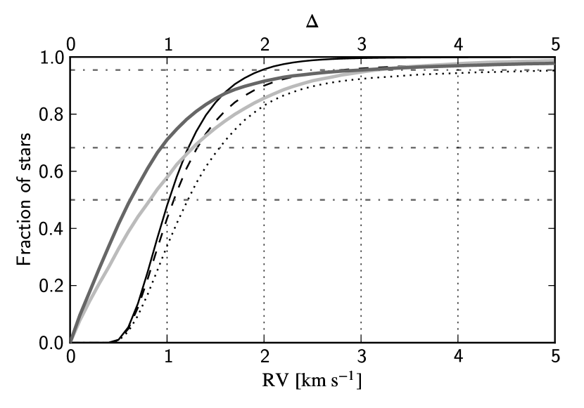
The VDR3 database consists of 344,924 entries including the already published data from the first and second releases. Out of those there are 295,618 database entries with $\mathrm{S/N}>20$ and further exclusion of the second-order-light-plagued data from the first release leaves 279,120 observations of 249,980 different stars. This subset serves as the basis of this paper. Repeated observations were identified by matching Two Micron All Sky Survey (2MASS) identifiers. For a small set of stars with missing 2MASS identifiers we compared their coordinates and matched stars that were not more than $5^{\prime\prime}$ apart. All matching cases were visually checked on the DSS plates to ensure the catalog entries indeed belong to the same star. We decided to exclude the data from the first release because the classification of those spectra is unreliable due to strong continuum variations and their RV measurements are usually significantly less accurate than the RVs of spectra recorded later. Cumulative distributions of RV errors for different data sets are shown in Figure 1. The median error of the selected subset stands at just over $1\,\mathrm{km\ s^{-1}}$ and RVs of 95% of all cold single stars are measured to better than $2\,\mathrm{km\ s^{-1}}$. There is a notable improvement in RV accuracy compared to the second data release. The same figure also shows the distribution of applied zero-point corrections. In roughly two thirds of all cases this correction is smaller than the error of the measured RV, although in some cases the correction can be an order of magnitude larger than the RV errors.

3. Repeated Observations

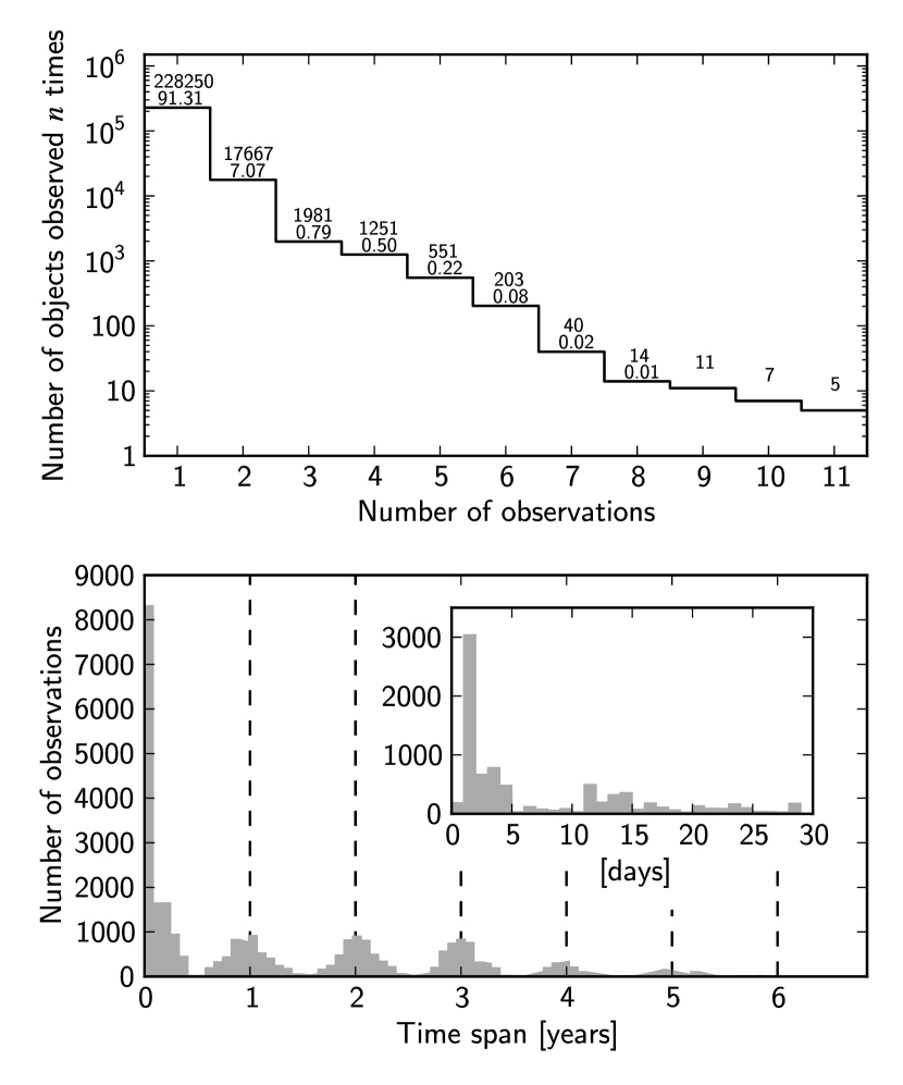
In order to identify any stars with variable RVs, more than one observation of the same stars is needed. The RAVE survey is primarily focused on the acquisition of as many different targets as possible. Re-observations of the same stars are done for stability and quality check purposes and also to allow for the determination of the fraction of stars with variable RVs. Nevertheless, at about 9% of all observations the number of stars that were observed more than once is still high (Figure 2). Altogether, 21,730 stars were observed more than once in the selected subsample. Most of the repeats were observed in the following few days with a strong peak at a day after the previous observation.

Figure 2.— Upper diagram shows the number of objects observed $n$ times along with the fraction that this number represents in the whole sample of 279,120 stars. The lower diagram shows the distribution of the time span between the consecutive observations of the same objects.

The stability of RVs is shown in Figure 1. The thick dark gray line shows the distribution of average differences between the RV measurements and their weighted average ($\overline{\mathrm{RV}}$) in terms of individual errors,

$$\Delta=\frac{1}{N}\sum_{i}^{N}\frac{|\mathrm{RV}_{i}-\overline{\mathrm{RV}}|}{\sigma_{i}},$$ (1)

for all repeatedly observed normal single stars with $\mathrm{S/N}>20$ (same set as used for the thin solid line in Figure 1). $N$ indicates the number of observations for a given star. A long tail of the distribution toward the larger values of $\Delta$ is indeed not an observational error but indicates the presence of the stars with variable RVs.

To establish a quantitative criterion for RV variability we defined the following function. We denoted two RVs and their errors measured for the same star at two different times as $(\mathrm{RV}_{1},\sigma_{1})$ and $(\mathrm{RV}_{2},\sigma_{2})$. The squares of the RV errors $\sigma_{i}^{2}$ can be treated as variances of the Gaussian distributions with the mean values $\mathrm{RV}_{i}$. If we would randomly pick two samples from each of these distributions, the probability that the pick from the second one is greater than the pick from the first one is equal to

$$P(2>1) = \frac{1}{\sqrt{2\pi\sigma_{1}^{2}}}\frac{1}{\sqrt{2\pi\sigma_{2}^{2}}}$$

$$\int_{-\infty}^{\infty}\!\int_{-\infty}^{y}\!e^{-\frac{(x-\mathrm{RV}_{1})^{2}}{2\sigma_{1}^{2}}}e^{-\frac{(y-\mathrm{RV}_{2})^{2}}{2\sigma_{2}^{2}}}dxdy.$$

The double integral can be simplified by introducing a new variable $u=(x-\mathrm{RV}_{1})/\sqrt{2}\sigma_{1}$ and evaluating the integration over $x$,

$$P(2>1)= \frac{1}{\sqrt{2\pi\sigma_{2}^{2}}} \int_{-\infty}^{\infty}\!\frac{1}{2}\left[1+\mathrm{erf}\left(\frac{y-\mathrm{RV}_{1}}{\sqrt{2}\sigma_{1}}\right)\right]$$

$$e^{-\frac{(y-\mathrm{RV}_{2})^{2}}{2\sigma_{2}^{2}}}dy,$$

where $\mathrm{erf}$ is the standard error function. By using the following identity,

$$\int_{-\infty}^{\infty}\!e^{-(ax+b)^{2}}\mathrm{erf}(cx+d)dx=\frac{\sqrt{\pi}}{a}\mathrm{erf}\left(\frac{ad-bc}{\sqrt{a^{2}+c^{2}}}\right),$$ (4)

we can write a simple expression for the probability in question,

$$P(2>1)=\frac{1}{2}\left[1+\mathrm{erf}\left(\frac{\mathrm{RV}_{2}-\mathrm{RV}_{1}}{\sqrt{2(\sigma_{1}^{2}+\sigma_{2}^{2})}}\right)\right].$$ (5)

If the difference in the numerator of the error function is zero (both RVs are the same), the probability is equal to $1/2$ and goes toward 1 for pairs with very different $\mathrm{RV}$s and comparably small $\sigma$s. If $\mathrm{RV}_{1}$ is greater than $\mathrm{RV}_{2}$, than the probability $P$ will be less than $1/2$. Since we are only interested if the RV changed between measurements, we can always label the greater of both RVs with index $2$ without the loss of generality. The nature of error function makes it hard to tell the difference between two pairs with relatively large RV differences because the value of the error function will always be very close to $1$ in such cases. It is more convenient to define a new function involving the logarithm of the function $P$,

$$p_{\mathrm{log}}=-\log_{10}(1-P).$$ (6)

The calculation of the logarithm in this function where the difference $1-P\approx 10^{-15}$ is troublesome due to double precision floating point limitations. To prevent any numerical inconsistencies the upper limit of the $p_{\mathrm{log}}$ criterion was set to 14 in the subsequent calculations.

Figure 3.— $p_{\mathrm{log}}$ from Eq. 6 as a function of difference $\mathrm{RV}_{2}-\mathrm{RV}_{1}$ in units of $\sigma_{1}$. Different line styles correspond to different values of $\sigma_{2}$, also in units of $\sigma_{1}$.

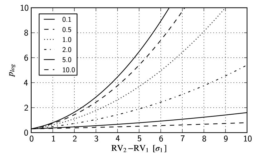
The function $p_{\mathrm{log}}$ is shown in Fig. 3 for several different error ratios. For example, if both errors are the same $(\sigma_{1}=\sigma_{2})$ and the $\mathrm{RV}$s are roughly $4\sigma_{1}$ apart, the value of the function $p_{\mathrm{log}}$ will be a little less than three, corresponding to the value of $P=0.998$ so the large majority of the values from the second distribution are greater than the values from the first. The probability that the radial velocity changed from one observation to another is relatively high. On the other hand, if $p_{\mathrm{log}}<2$, the variability is questionable and if $p_{\mathrm{log}}<1$, the radial velocity variability is insignificant. In comparison, the lower limit of the variability criterion given in Pourbaix et al. (2005) for stars observed twice and with equal RV errors for both measurements is $p_{\mathrm{log}}=2.87$.

4. Catalog of SB1 candidates

We have examined a sample of 21,730 objects that were observed at least twice. We excluded all objects whose spectra are morphologically different from spectra of single stars since the described RV extraction method does not give reliable results in such cases, including double-lined spectroscopic binaries. All such objects were identified using the classification method described in Paper I. The method systematically examines the properties of the cross-correlation function between each observed spectrum and a pre-calculated synthetic template and according to those properties groups similar spectra together. Among the excluded classes were spectra with observational or reduction errors (problematic continuum normalization, for example), hot stars whose Paschen series lines are too wide for precise RV measurement and intrinsically peculiar stars (stars with active chromospheres, emission line stars, etc.). The selection reduced the number of stars in the sample to 20,027.

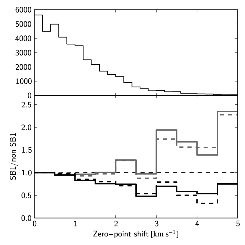
We calculated the $p_{\mathrm{log}}$ variability criterion for all stars from this sample using the RV measurements and their errors as given in the RAVE database. In cases where more than two observations were available, the pair with the highest value of the criterion was considered. The inspection of a few stars with the largest number of repeated observations revealed that in some cases only one or two of the RV measurements were not consistent with the averaged RV. We note that some of the observations responsible for the RV variability have large values of the zero-point correction which is usually very small (Section 2). The comparison of the number of SB1 candidates with zero-point shift in some interval to the rest of the repeatedly observed stars in the same interval showed that there was a significant overdensity of SB1 candidates in the region where at least one of the two RV measurements in the pair was corrected for a relatively high amount (Figure 4).

Figure 4.— Bottom diagram shows the ratio between the number of SB1 candidates vs. the number of the rest of repeatedly observed stars as a function of zero-point shift. All histograms are normalized so that the first bin equals 1. Gray lines show the initial calculation where the zero-point uncertainty is not included ($k=0$ in Equations 7,8), whereas black lines show the same distribution for $k=0.5$. SB1 candidates in both cases are considered all pairs with $p_{\mathrm{log}}>3$ (full lines) and $p_{\mathrm{log}}>4$ (dashed-lines). The upper diagram shows the distribution of zero-point shifts for the pairs of observations with the highest variability criterion for all stars observed more than once.

Such spurious detections would contaminate the statistics of discovered SB1 candidates. To account for this systematic error we recalculated the variability criterion with the adjusted error estimate:

$$\sigma=\sqrt{\sigma_{\mathrm{RV}}^{2}+\sigma_{\mathrm{ZP}}^{2}},$$ (7)

where

$$\sigma_{\mathrm{ZP}}=k*\mathrm{RV}_{\mathrm{ZP}},$$ (8)

so the error in zero-point shift is proportional to the shift in this approximation. Equation 7 is only valid if RV and zero-point error estimates are uncorrelated. This was checked and indeed holds true. The coefficient $k=0.5$ was selected so that it fully eliminates the SB1 overdensity at large zero-point shifts. It was also intentionally set high enough so that the ratio of SB1 candidates confirmed with the adjusted error estimate compared to the ones before this test is a decreasing function of the value of the zero-point correction. One expects that because high values of zero-point shifts are the least trustworthy and include the highest fraction of potential false positives. The overall number of SB1 candidates is not much affected by the selected value of $k$, since the majority of all RVs have relatively small zero-point corrections (in only 5% of the cases they exceed $3\,\mathrm{km\ s^{-1}}$ and anyway are smaller than the RV errors, see Figure 1).

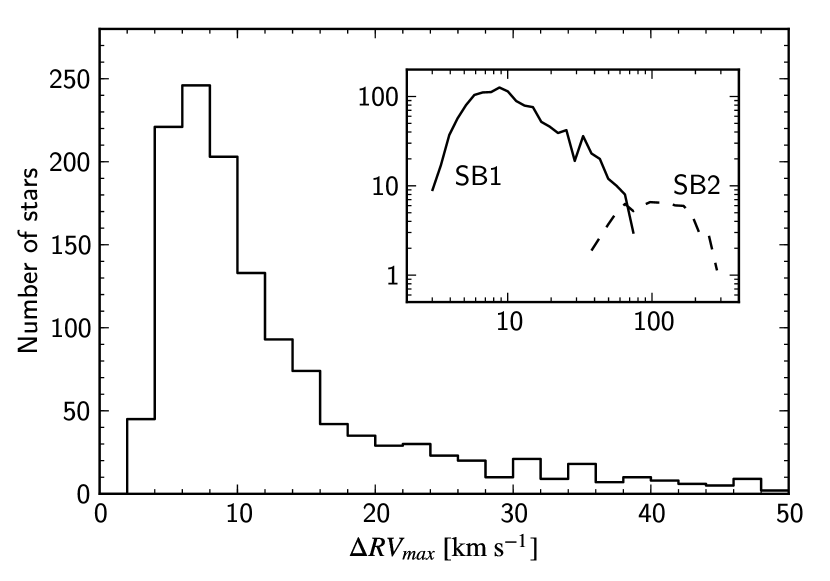
Altogether, 1333 or 6.6% of the stars have $p_{\mathrm{log}}\geq 3$ and were identified as potential SB1 candidates. The summary of the number of discovered candidates versus the number of observations is given in Table 1. Since the limiting value of $p_{\mathrm{log}}=3$ is arbitrary, $p_{\mathrm{log}}=2,4$ are given for comparison. It is evident that for $p_{\mathrm{log}}=2$ the number of SB1 candidates becomes unrealistically high, making the $p_{\mathrm{log}}=3$ a plausible lower limit for the variability criterion. The efficiency of the detection is $\sim 6$% for twice observed star but it grows steadily toward $\sim 15$% for stars observed five or six times. There are too few candidates with more observations to draw any conclusions. The number of identified candidates gives only a lower limit of spectroscopic binaries in the observed sample and selection criteria were indeed set restrictively to avoid as much potential false positives as possible and also to account for the fact that the RV error estimates might not always be Gaussian. With the maximal time span between re-observations at around 2000 days it cannot be expected that systems with significantly longer periods are detectable. More so, in long period systems the RV amplitudes become too small to be detectable and most of the SB1 candidates were observed for the second time only days after the first observation. The distribution of RV differences between measurements is shown in Figure 5. Most frequently the variations were small, around the value of $6\,\mathrm{km\ s^{-1}}$. The distribution falls quickly after $10\,\mathrm{km\ s^{-1}}$ but extends all the way to over $160\,\mathrm{km\ s^{-1}}$. All single-lined objects with high RV shifts are particularly interesting for further investigation due to the possibility of the presence of massive and faint objects. The distribution of RV shifts was also compared to the distribution of separations between the components of the identified SB2 candidates (Figure 5). The data for velocity separations were taken from the list of preliminary solutions for 1040 SB2 objects found in the RAVE catalog (partially described in Paper I). The distribution shown on the plot was scaled compared to the SB1 distribution so that the effective number of stars from which the selection was done is the same for both types. The efficiency of SB2 detection becomes high at the point where the number of identified SB1 objects gets low.

Figure 5.— Distribution of maximum changes of radial velocity between measurements for the identified SB1 candidates. The smaller diagram shows the same distribution in the logarithmic scale along with the preliminary normalized distribution of separations between components of identified SB2 candidates (dashed line).

Table 1Number of SB1 Candidates for Different Values of $p_{\mathrm{log}}$

	$p_{\mathrm{log}}=2$		$p_{\mathrm{log}}=3$		$p_{\mathrm{log}}=4$
${N_{obs}}$	$N$	${N/N_{all}}$	$N$	${N/N_{all}}$	$N$	${N/N_{all}}$
2	1438	0.09	919	0.06	706	0.04
3	263	0.15	166	0.09	127	0.07
4	230	0.20	127	0.11	91	0.08
5	147	0.28	71	0.14	47	0.09
6	52	0.28	33	0.18	22	0.12
7	17	0.42	7	0.17	5	0.12
8	7	0.78	1	0.11	1	0.11
9	8	0.73	4	0.36	3	0.27
10	6	0.86	3	0.43	2	0.29
11	3	0.75	2	0.50	0	0.00

Figure 6.— Upper left panel: $\{T_{\mathrm{eff}},\log g\}$ diagram for a sample of identified SB1 candidates. The variability criterion $(p_{\mathrm{log}})$ is represented with different shades of gray where darker tones and bigger markers correspond to greater chance of RV variability. The dashed line roughly divides giants mostly from the red clump (RC) region and main-sequence (MS) stars. The error bars represent typical uncertainties of both parameters. Upper right panel: photometrically variable stars from the VSX catalog (see the text) and suspected SB2 objects among the identified SB1 candidates. Lower left panel: SB1 candidates with color-coded distances from Zwitter et al. (2010) and tone values as in the previous diagram. Here, only the size of markers corresponds to the value of $p_{\mathrm{log}}$ to avoid confusion. Isochrones for $\mathrm{[M/H]}=-0.2$ spanning $9.0\textrm{--}10.0$ in log age with $0.2$ steps by Marigo et al. (2008) and Girardi et al. (2010). Lower right panels: normalized distributions of effective temperature, metallicity, 2MASS $M_{J}$ magnitude and S/N for non-peculiar single stars of the whole RAVE sample (blue), stars observed more than once (green) and SB1 candidates (red).

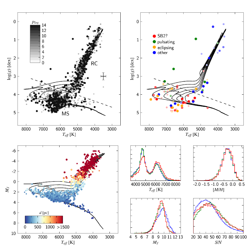
The $\{T_{\mathrm{eff}},\log g\}$ diagram of all SB1 candidates and various distributions are shown in Figure 6. The distribution of effective temperature of stars observed multiple times has two distinct peaks at around $4500\,\mathrm{K}$ for the red clump stars and $6000\,\mathrm{K}$ for the main sequence dwarfs, same as in the overall RAVE sample. The S/N of the re-observed stars is somewhat higher than in the general population. The reason is that slightly brighter stars were observed more frequently than the faint ones. There are more SB1 dwarf candidates than giant candidates, which is also apparent from the distribution of effective temperatures for the SB1 candidate sample. The ratio of giants to dwarfs in the whole RAVE sample is around 57:43, while the same ratio for the SB1 candidates is close to 50:50. This is an expected result. SB1 candidates roughly fall into two groups: main sequence stars with masses $\sim 1-1.2\ M_{\odot}$ and red clump giants with masses slightly larger than the first group (based on isochrones by Marigo et al. (2008)). The important difference between the two groups is approximately an order of magnitude larger radii of giant stars. This implies that the smallest binary orbits than can host giant stars must be larger than the orbits of main sequence stars due to Roche lobe radius limits (see for example Eggleton (1983)). Consequently, the periods of SB1 binaries that host giant stars will be longer and average RV shifts will be smaller and therefore harder to detect.

The distribution of metallicity is relatively wide since RAVE observes field stars representing the general population of thin and thick disks. The metallicity of SB1 candidates does not differ from the rest of the stars meaning that SB1s are also scattered throughout both disks. Due to RAVE’s narrow magnitude range, dwarf candidates are mostly limited to the thin disk, while giants also reach into the Galaxy’s thick disk (lower left panel of Figure 6; see also Zwitter et al. (2010) for further discussion on distances).

Visual inspection of spectra revealed that 43 SB1 candidates could in fact be double-lined spectroscopic binaries if observed at higher resolutions or at more favorable phases (red markers in the upper right panel of Figure 6). The assumption is based on their slightly asymmetric and widened lines but the effect is too small for more confident confirmation. Note that atmospheric parameters for such stars are generally incorrect since the pipeline always assumes that the observed spectrum belongs to a single star and models the binary spectrum with this assumption. Nevertheless, the general region (dwarf/giant) of the solution is correct since the most affected parameter is rotational velocity while the effective temperature and surface gravity are not very sensitive to the apparent slight line broadening that is produced by the shift. Most of these stars are close to the main sequence.

We do not wish to attempt to infer binary orbits for those stars with the highest number of observations. While it is possible to derive orbital parameters for stars with six or more observations in theory, the precision of the calculated solution also depends on how well the measured points are distributed along the orbital phase, on the uncertainty of RVs and so on. We tried to fit the orbits for some stars, but none of the solutions turned out to be reliable.

The catalog of all stars with variable RVs will be made publicly available through the CDS service.

4.1. Comparison to other catalogs

Figure 7.— Spectroscopic orbits from $S_{B^{9}}$ catalog and RAVE RVs (black markers) for each star. The phase uncertainty is calculated from a given period error. The radial velocity data for HIP 5438 from Andersen et al. (1988), HIP 44124 from Goldberg et al. (2002), BD -21 3873 from Smith et al. (1997), BD -01 3022, HIP 43527 and CPD -64 4333 from Udry et al. (1998), HIP 75718 and HIP 86400 from Tokovinin (1991), HIP 59750 and HIP 55022 from Carney et al. (2001), BD -01 3141 from Griffin (1994), HIP 65982 from Latham et al. (2002), Cl* NGC 2477 HART 2064 and Cl* NGC 2477 HART 8017 from Eigenbrod et al. (2004), HIP 42368 from Griffin (2004), HIP 64219 from Duquennoy & Mayor (1991), HIP 50796 from Torres (2006), BD -18 5091 from Carquillat & Prieur (2007), BD -20 3310, BD -15 3197, CD -23 9811, CD -27 9246, CD -27 9317, CD -26 9873, CD -25 10022, BD -20 3997 and HIP 22761 from Griffin (2006) and Cl* Ruprecht 46 MMU 2191 from Mermilliod et al. (2007).

We compared the list of identified SB1 candidates to the list of known photometric variables in the VSX catalog (Watson, 2006, Version 02-Jan-2011) and to the ninth catalog of spectroscopic binary orbits ($S_{B^{9}}$; Pourbaix et al., 2004). Within the VSX there are 36 stars matching our list. Out of those, 10 are pulsating variables, 14 eclipsing binaries and 20 unclassified variables. Their positions on the $\{T_{\mathrm{eff}},\log g\}$ diagram are shown in Figure 6. RV variations measured for pulsating variables are generally lower than $30\,\mathrm{km\ s^{-1}}$ (Aerts et al., 2010), but can be as high as $\sim 100\,\mathrm{km\ s^{-1}}$ for some types (Gorynya et al., 1998; Sanford, 1949). In our case, the two leftmost green dots in the upper right panel of Figure 6 are an RR Lyrae star (hotter) and a Cepheid with the RV amplitude of at least $21\,\mathrm{km\ s^{-1}}$ and $46\,\mathrm{km\ s^{-1}}$, respectively. The rest of the pulsating variables mostly lie above the dwarf-giant border. Of course, there is a possibility that some of the rest of the identified SB1 candidates are pulsating variables rather than binary stars. Conversely, eclipsing binaries and potential SB2 candidates are generally (taking atmospheric parameter uncertainties into account) among main sequence dwarfs. This supports the assumption from Paper I and also agrees with the sample of eclipsing binaries from Torres et al. (2010) where the majority of all analyzed systems are pairs of main-sequence stars.

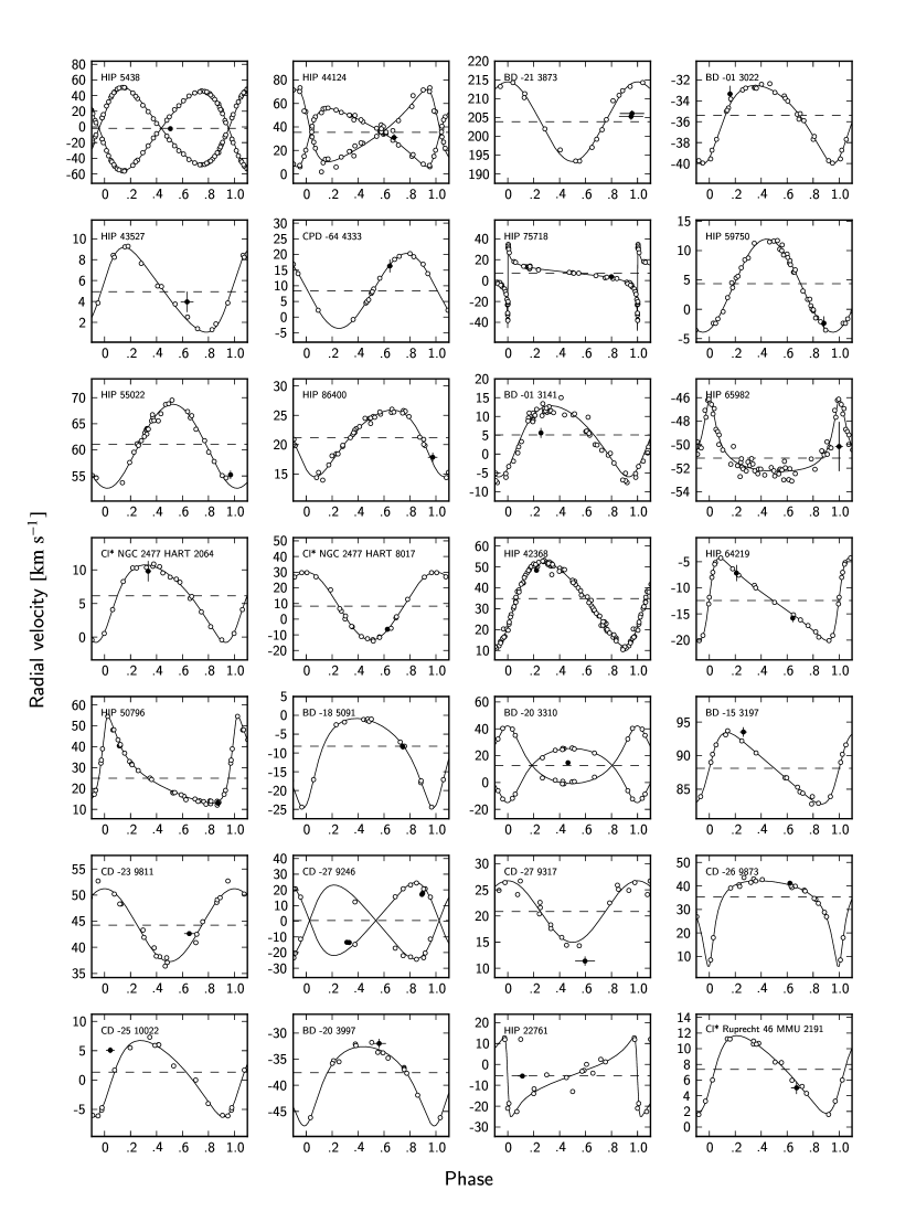
The comparison of the whole RAVE sample to the $S_{B^{9}}$ catalog yielded 56 matches but only three of those stars were observed more than once, two of them twice, and one four times. For the sake of testing the accuracy of RVs, single observations were compared to known orbits as well. We selected 26 orbital solutions for which the difference between the published periastron time and the date of the RAVE observation were closer than 100 periods apart in order to avoid errors caused by period propagation. There are two exceptions with a difference of 343 and 448 periods where the correspondence between the RAVE measurements and the RV curve was still acceptable. In other cases several thousand periods have passed between the given periastron time and the time of the RAVE measurement. Orbital solutions with RAVE measurements are shown in Figure 7. There are four known SB2 systems among the selected sample. RAVE spectra of HIP 5438 and HIP 44124 were recorded close to the half phase and so both RVs are near the systemic $\gamma$ velocity. The RV amplitudes of both systems are large enough that both systems would be detected as SB2 if observed at more favorable phases. System BD -20 3310 was observed close to the apastron but again the measured RV is near the center-of-mass RV because spectra of both components contribute to the composite so the peak of the correlation function lies in the middle of both components. System CD -27 9246 was observed four times, but coincidentally at only two different phases. All four RVs correspond to one component of the system. Other RAVE RVs are close to the predicted values and in most cases within the error bars, giving additional reassurance to the error estimates. In three cases, BD -21 3873, BD -01 3141, and HIP 22761, the measured RVs lie very close to the $\gamma$ velocities of the system, very similar to the three cases of known SB2 systems. The reason for this seems to be different in each case. A poor match in the case of HIP 22761 (HD 31341) is most likely caused by confusion with another star due to an erroneous entry in the catalog. The $S_{B^{9}}$ catalog cites Griffin (2006) as the source, but the paper actually reports about the observation of the star HD 31341B, also known as HIP 22766. The mismatch in BD -21 3873 could be caused by an improper phase determination of the two RAVE measurements, since the phase inaccuracy in this case is the largest of all examples. In the case of BD -01 3141, a possible secondary component might only be observable at longer wavelengths because of its potentially low surface temperature. The reference paper (Griffin, 1994) states that all observations were performed on instruments capable of reaching wavelengths up to $\sim 5200\,$Å which is relatively far from RAVE’s spectral domain so there is a chance that the additional component was not present there.

5. Discussion and conclusions

We analyzed 20,027 stars observed multiple times by the RAVE spectroscopic survey in the $\sim 6$ year span between 2004 and 2010 with RV and atmospheric parameter estimates provided by the RAVE parameter estimation pipeline. Prior to the RV analysis we classified all spectra and filtered out those with peculiar features (e.g., emission line objects, double-lined binaries, spectra with observational errors, etc.) whose measured parameters are not reliable, obtaining a list of only normal single stars. In order to detect stars with variable RVs, we defined a variability criterion (Equation (5)), assuming that RV errors are Gaussian and taking the RV error and zero-point shift of individual measurements into account. In the observed sample, we identified 1333 objects with large enough changes in radial velocities to be identified as SB1 candidates. As summarized in Table 1, the fraction of discovered SB1 candidates is a function of the number of observations. Only 6 % of twice observed stars were detected as SB1 candidates. This fraction grows with the number of observations and saturates at around 10%-15% for stars with five or six observations, depending on the selected lower limit of the variability criterion. This number represents the lower limit for the overall fraction of stars with variable RVs present in the RAVE sample.

The distribution of maximal differences between the RVs for repeatedly observed stars (Figure 5) has a strong peak just below $10\,\mathrm{km\,s^{-1}}$. At smaller velocities the number of detected SB1 candidates quickly vanishes. The reason is a restriction on the $p_{\mathrm{log}}$ criterion that is required to be greater than 3 for sufficiently confident variability confirmation. Even in cases with the lowest values of RV errors (Figure 1) this criterion is not met if the two measurements are closer together than $\sim 3.5\,\mathrm{km\,s^{-1}}$ (Figure 3) which explains the sharp falloff below $4\,\mathrm{km\,s^{-1}}$. The same distribution was plotted for stars where $p_{\mathrm{log}}>4$ and the falloff was even stronger there which gives additional confirmation to the source of this feature. It should be noted that zero-point shifts (Figure 1) are in most cases well below the velocities where the detection becomes significant and are not the source of inaccuracies. On the other side of the distribution, there is an evident exponential falloff of detected candidates. This feature is expected to be real and not a selection effect. Systems with larger RV amplitudes most likely have shorter periods and therefore the detection efficiency for these cases is proportionally higher than at the lower velocity end. The distribution also extends into the SB2 region for which it was shown (Paper I) that the detection efficiency is very high at separations above $50\,\mathrm{km\,s^{-1}}$. It is hard to infer the periods of the SB1 candidates since mostly only two observations are available, but from the distribution of the time spans between observations it can be concluded that periods are most likely not significantly longer and so fall into the short end of the period distribution given in Duquennoy & Mayor (1991) or Raghavan et al. (2010). A detailed population study of both types of binaries (SB1 and SB2) and their influence on the general RV distribution of the RAVE stars will be a subject of the third paper regarding binaries in the RAVE survey.

The $\{T_{\mathrm{eff}},\log g\}$ diagram of SB1 candidates derived from the spectroscopic parameters of stars gives a similar picture as RAVE’s general population. The distribution of metallicities of SB1 candidates is the same as the distribution of metallicities of the general population which means that binaries are well mixed among the field stars. Similarly to the overall RAVE sample, the distribution of effective temperatures has two distinct peaks that correspond to main sequence stars and to the red clump giants with masses only slightly larger than the former group. There is a deficiency of SB1 candidates from the giant group compared to the dwarfs. It can be explained by comparing the typical radii of stars in both groups. Radii of giants in the observed sample are roughly an order of magnitude larger than the radii of main sequence stars. Therefore, binary orbits in which giants can exist (due to Roche lobe limits) must be on average larger than the orbits of main sequence stars so the orbital periods are longer and consequently RV shift smaller and more unlikely to be detected.

Comparison of the SB1 candidate list with the VSX catalog of photometrically variable stars yielded several hits with some stars being pulsating variables rather than spectroscopic binaries. The RV amplitudes of some types of pulsating variables can be as high as few $10\,\mathrm{km\,s^{-1}}$. There is some probability that some of the stars from our SB1 candidate list are pulsating but it should be negligibly low. For example, the fraction of Cepheids and RR Lyrae stars (variables with high RV variations) in the Hipparcos catalog (Perryman et al., 1997) is less than 0.4 %. The selection of stars in the RAVE’s input catalog is unbiased (with the exception of stellar magnitudes) so most of the observed stars are not in any unstable transiting phases of their lives. Among the photometrically variable stars are also several eclipsing binaries. Most of them lie close to the main sequence on the HR diagram. We also identified some potential SB2 candidates in our SB1 candidate list. They cannot be confirmed since they do not have a clear double-lined signature in their spectra, but time dependent asymmetries in spectral lines indicate that higher resolution spectra might be able to resolve two components. All of these objects also lie close to the main sequence which supports the argument that SB2 objects mostly consist of two main sequence stars and pairs of equally bright giants forming an SB2 system are rare.

There are 26 stars in the catalog of spectroscopic binary orbits ($S_{B^{9}}$) for which RAVE has at least one observation and the difference between the given time of periastron and the RAVE observation time is shorter than 100 epochs to ensure that the propagated period error is small enough. In most cases the agreement between the calculated RV curves and RAVE RVs is within the error estimates which confirms the precision of the RVs. Among the selection are four known SB2 objects. In three of those cases, the RAVE RV is close to the $\gamma$ velocity of the system which is expected because the peak of the correlation function that determines the RV is between both Doppler-shifted components. Conversely, in three other cases that are cataloged as SB1 objects, RAVE radial velocities are close to the systemic velocity and not near the calculated RV curve. This might implicate the presence of a still undiscovered bright secondary component.

References

- Abt & Willmarth (1999) Abt, H. A. & Willmarth, D. W. 1999, ApJ, 521, 682
- Aerts et al. (2010) Aerts, C., Christensen-Dalsgaard, J., & Kurtz, D. W. 2010, Asteroseismology (Berlin: Springer)
- Andersen et al. (1988) Andersen, J., Clausen, J. V., Nordstrom, B., Gustafsson, B. & Vandenberg, D. A. 1988, A&A, 196, 128
- Bate (2009) Bate, M. R. 2009, MNRAS, 392, 590
- Boeche et al. (2010) Boeche, C., et al. 2010, BAAS, 215, 456.09
- Carney et al. (2001) Carney, B. W., Latham, D. W., Laird, J. B., Grant, C. E. & Morse, J. A. 2001, AJ, 122, 3419
- Carquillat & Prieur (2007) Carquillat, J.-M. & Prieur, J.-L. 2007, Astron. Nachr., 328, 527
- Duquennoy & Mayor (1991) Duquennoy, A. & Mayor, M. 1991, A&A, 248, 485
- Eggleton (1983) Eggleton, P. P. 1983, ApJ, 268, 368
- Eigenbrod et al. (2004) Eigenbrod, A., Mermilliod, J.-C., Clariá, J. J., Andersen, J. & Mayor, M. 2004, A&A, 423, 189
- Fischer & Marcy (1992) Fischer, D. A. & Marcy, G. W. 1992, ApJ, 396, 178
- Girardi et al. (2010) Girardi, L., et al. 2010, ApJ, 724, 1030
- Goldberg et al. (2002) Goldberg, D., Mazeh, T., Latham, D. W., Stefanik, R. P., Carney, B. W. & Laird, J. B. 2002, AJ, 124, 1132
- Gorynya et al. (1998) Gorynya, N. A., Samus’, N. N., Sachkov, M. E., Rastorguev, A. S., Glushkova, E. V. & Antipin, S. V. 1998, Astron. Lett., 24, 815
- Griffin (1994) Griffin, R. F. 1994, The Observatory, 114, 231
- Griffin (2004) Griffin, R. F. 2004, The Observatory, 124, 97
- Griffin (2006) Griffin, R. F. 2006, MNRAS, 371, 1159
- Lada (2006) Lada, C. J. 2006, ApJ, 640, L63
- Latham et al. (2002) Latham, D. W., et al. 2002, AJ, 124, 1144
- Marigo et al. (2008) Marigo, P., Girardi, L., Bressan, A., Groenewegen, M. A. T., Silva, L. & Granato, G. L. 2008, A&A, 482, 883
- Mason et al. (2009) Mason, B. D., Hartkopf, W. I., Gies, D. R., Henry, T. J. & Helsel, J. W. 2009, AJ, 137, 3358
- Matijevič et al. (2010) Matijevič, G. et al. 2010, AJ, 140, 184, (Paper I)
- Mermilliod et al. (2007) Mermilliod, J.-C., Andersen, J., Latham, D. W. & Mayor, M. 2007, A&A, 473, 829
- Munari et al. (2005) Munari, U., Sordo, R., Castelli, F. & Zwitter, T. 2005, A&A, 442, 1127
- Nordström et al. (2004) Nordström, B., et al. 2004, A&A, 418, 989
- Perryman et al. (1997) Perryman, M. A. C., et al. 1997, A&A, 323, 49
- Pourbaix et al. (2004) Pourbaix, D., et al. 2004, A&A, 424, 727
- Pourbaix et al. (2005) Pourbaix, D., et al. 2005, A&A, 444, 643
- Raghavan et al. (2010) Raghavan, D., et al. 2010, ApJS, 190, 1
- Sana et al. (2009) Sana, H., Gosset, E. & Evans, C. J. 2009, MNRAS, 400, 1479
- Sanford (1949) Sanford, R. F. 1949, Contrib. Mount Wilson Obs. / Carnegie Inst. of Washington, 757, 1
- Siebert et al. (2011) Siebert, A., et al. 2011, accepted
- Smith et al. (1997) Smith, V. V., Cunha, K., Jorissen, A., & Boffin, H. M. J. 1997, A&A, 324, 97
- Sommariva et al. (2009) Sommariva, V., Piotto, G., Rejkuba, M., Bedin, L. R., Heggie, D. C., Mathieu, R. D. & Villanova, S. 2009, A&A, 493, 947
- Steinmetz et al. (2006) Steinmetz, M., et al. 2006, AJ, 132, 1645
- Tokovinin (1991) Tokovinin, A. A. 1991, A&AS, 91, 497
- Tonry & Davis (1979) Tonry, J. & Davis, M. 1979, AJ, 84, 1511
- Torres (2006) Torres, G. 2006, AJ, 131, 1022
- Torres et al. (2010) Torres, G., Andersen, J. & Giménez, A. 2010, A&A Rev., 18 ,67
- Udry et al. (1998) Udry, S., Jorissen, A., Mayor, M. & Van Eck, S. 1998, A&AS, 131, 25
- Watson (2006) Watson, C. L. 2006, Society for Astronomical Sciences Annual Symposium, Vol. 25, 47
- Zwitter et al. (2008) Zwitter, T., et al. 2008, AJ, 136, 421
- Zwitter et al. (2010) Zwitter, T., et al. 2010, A&A, 522, 54