Pointwise Adaptive M-estimation in Nonparametric Regression

Abstract

This paper deals with the nonparametric estimation in heteroscedastic regression $Y_{i}=f(X_{i})+\xi_{i},\>i=1,\ldots,n$, with incomplete information, i.e. each real random variable $\xi_{i}$ has a density $g_{i}$ which is unknown to the statistician. The aim is to estimate the regression function $f$ at a given point. Using a local polynomial fitting from M-estimator denoted $\hat{f}^{h}$ and applying Lepski’s procedure for the bandwidth selection, we construct an estimator $\hat{f}^{\hat{h}}$ which is adaptive over the collection of isotropic Hölder classes. In particular, we establish new exponential inequalities to control deviations of local M-estimators allowing to construct the minimax estimator. The advantage of this estimator is that it does not depend on densities of random errors and we only assume that the probability density functions are symmetric and monotonically on ${\mathbb{R}}_{+}$. It is important to mention that our estimator is robust compared to extreme values of the noise.

Key words: adaptation, Huber function, Lepski’s method, M-estimation, minimax estimation, nonparametric regression, robust estimation, pointwise estimation.

AMS 2000 subject classification: Primary 62G08; secondary 62G20, 62G35.

¹Université Aix-Marseille 1, LATP
39, rue F. Joliot Curie, 13453 Marseille Cedex 13, France.
E-mail: chichign@cmi.univ-mrs.fr

1 Introduction

Let the statistical experiment be generated by the observation
$Z^{(n)}=(X_{i},Y_{i})_{i=1,...n},n\in{\mathbb{N}}^{*}$, where each $(X_{i},Y_{i})$ satisfies the equation

$$Y_{i}=f(X_{i})+\xi_{i},\quad i=1,\ldots,n.$$ (1.1)

Here $f:[0,1]^{d}\rightarrow\mathbb{R}$ is an unknown function to be estimated at a given point $x_{0}\in[0,1]^{d}$ from the observation $Z^{(n)}$.

The real random variables $(\xi_{i})_{i\in{1,\ldots,n}}$ (the noise) are supposed to be independent and each variable $\xi_{i}$ has a symmetric density $g_{i}(\cdot)$, with respect to the Lebesgue measure on $\mathbb{R}$. We also assumed that $g_{i}$ is monotonically on ${\mathbb{R}}_{+}$ for any $i$.

The design points $(X_{i})_{i\in{1,...,n}}$ are independent and uniformly distributed on $[0,1]^{d}$. The random vectors $(X_{i})_{i\in{1,...,n}}$ and $(\xi_{i})_{i\in{1,\ldots,n}}$ are independent.

Along the paper, the unknown function $f$ is supposed to be smooth, in particular, it belongs to an isotropic Hölder ball of functions $\mathbb{H}_{d}({\beta},L,M)$ (cf. Definition 1 below). Here ${\beta}>0$ is the smoothness of $f$, $L>0$ is the Lipschitz constant and $M$ is an upper bound of $f$ and its partial derivatives.

Motivation.

In this paper, the considered problem is the robust nonparametric estimation, i.e. the estimation of the regression function $f$ in the presence of a heavy-tailed noise (cf. [31] and [15]). Well-known examples are when the noise distribution is for instance Laplace (no finite exponential’s moment) or Cauchy (no finite order’s moments). Moreover, we assume that the noise densities $\big{(}g_{i}\big{)}_{i=1,...,n}$ are unknown to the statistician. This problem has popular applications, for example in relative GPS positioning (cf. [6]) or in robust image denoising (cf. [1]).

In parametric case, we consider $f$ as a constant parameter $\theta\in{\mathbb{R}}$. The use of empiric criteria is very popular, i.e. the minimization of the following contrast function $\rho$:

$$\hat{\theta}=\arg\min_{t\in[-M,M]}\sum_{i=1}^{n}\rho(Y_{i}-t),$$

The most famous contrast functions are the square function $\rho(z)=z^{2}$ ($\hat{\theta}$ become the empiric mean), the absolute value function $\rho(z)=|z|$ ($\hat{\theta}$ become the empiric mean) and the Huber function, as defined in (5.3), without an explicit expression of $\hat{\theta}$ (cf. [16]). It is well known that the square function leads to the empiric mean which does not fit with a heavy-tailed noise. Thus the square function is not suitable in the model (1.1).

In nonparametric estimation, we propose a local parametric approach (LPA) to estimate the regression function at a given point $x_{0}\in[0,1]^{d}$ in the model (1.1). We suppose that $f$ is locally almost polynomial (with degree $b\in{\mathbb{N}}$) and we use the parametric estimator on a neighborhood denoted $V_{x_{0}}(h)$ The parameter is reconstructed from the following criterion, for any $x_{0}\in[0,1]^{d}$ and $h\in[0,1]$

$$\hat{\theta}=\arg\min_{t\in[-M,M]^{N_{b}}}\sum_{i:X_{i}\in V_{x_{0}}(h)}\rho\big{(}Y_{i}-f_{t}(X_{i})\big{)}\>K\left(\frac{X_{i}-x_{0}}{h}\right).$$ (1.2)

where $f_{t}(\cdot)$ is a polynomial of degree $b$ with coefficients $t$, $K(\cdot)$ is a kernel function and $N_{b}$ is the number of partial derivatives of $f$ of order smaller than $b$. We refer to $\hat{f}^{h}(x_{0})=f_{\hat{\theta}}(x_{0})$ as the $\rho$-LPA estimator. It belongs to the family of M-estimators and it relies on a local scale parameter $h$, called the bandwidth. A crucial issue is the optimal choice of the parameter $h$. To adress it we use quite standard arguments based on the bias/variance trade-off (cf. (1.5) below) in minimax case and the Lepski’s rule for the data-driven selection in adaptation. First, since $f$ is smooth ($f\in\mathbb{H}_{d}({\beta},L,M)$, cf. Definition 1 below) we notice that

$$\exists\theta=\theta(f,x_{0},h)\in\Theta\big{(}M\big{)}:\quad b_{h}:=\sup_{x\in V_{x_{0}}(h)}\big{|}f(x)-f_{\theta}(x)\big{|}\leq Ldh^{\beta}.$$ (1.3)

We can choose $\theta$ as the coefficients of Taylor polynomial as defined in (2.6). Thus, if $h$ is chosen sufficiently small our original model (1.1) is well approximated inside of $V_{x_{0}}(h)$ by the “parametric” model

$${\cal Y}_{i}=f_{\theta}(X_{i})+\xi_{i},\quad\forall i\>:\>X_{i}\in V_{x_{0}}(h).$$ (1.4)

With this model, the $\rho$-LPA estimator $\hat{\theta}$ achieves the usual parametric rate of convergence $1/\sqrt{nh^{d}}$, where $nh^{d}$ is the number of the observations in the neighborhood $V_{x_{0}}(h)$ (See Theorem 1, Section 3).

This approach has been introduced by [19] and used for the first time in robust nonparametric estimation by [37], [13] and [12] to obtain asymptotic normality and minimax results. We also notice that Tsybakov[1982a,1982b,1983] obtained similar results to estimate the locally almost constant functions.

Minimax Estimation.

To guarantee good performance of the $\rho$-LPA estimator in the minimax sense, we assume that $\rho^{\prime}$ is bounded and Lipschitz. On the other hand, the Huber function satisfies these assumptions, making it suitable for our problem. Moreover, it is commonly used in practice (see for instance [29] and [6]). As for linear estimators (kernel estimators, least square estimators, etc.), a good choice of the bandwidth $h=\bar{h}_{n}(\beta,L)$ provides an optimal $\rho$-LPA estimator over the Hölder space $\mathbb{H}_{d}({\beta},L,M)$. Finally, $\bar{h}_{n}({\beta},L)=(L^{2}n)^{-\frac{1}{2\beta+d}}$ is chosen as the solution of the following bias/variance trade-off

$$\big{(}nh^{d}\big{)}^{-1/2}+Lh^{\beta}\rightarrow\min_{h}.$$ (1.5)

In the model (1.1), we show that the corresponding estimator $\hat{f}^{\bar{h}_{n}({\beta},L)}({x_{0}})$ achieves the rate of convergence $n^{-\beta/(2\beta+d)}$ (cf. Definition 2) for $f({x_{0}})$ on $\mathbb{H}_{d}({\beta},L,M)$ (See Theorem 1). We should point out that both the knowledge of $\beta$ and $L$ is required to the statistician in order to built the optimal bandwidth $\bar{h}_{n}(\beta,L)$.

Adaptive Estimation.

In nonparametric statistics, an important problem is the adaptation compared to the smoothness parameters $\beta$ and $L$ that are unknown in practice. This requests to develop a data-driven (adaptive) selection to choose the bandwidth. Then, the interesting feature is the selection of estimators from a given family (cf. [2], [22], [9]). In this context, several approaches to the selection from the family of linear estimators were recently proposed, see for instance [9], [10], [18] and the references therein. However, those methods strongly rely on the linearity property. Robust estimators are generally non-linear, there standard arguments (like the bias/variance trade-off) cannot be applied straightforwardly. For instance, [5] use the asymptotic normality of the median to approximate the model (1.1) by the wavelet sequence data and they use BlockJS wavelet thresholding for adaptation over Besov spaces with the integrated risk. Recently, [30] have considered the pointwise estimation for locally almost constant functions in the homoscedastic regression with a heavy-tailed noise. That corresponds to $\beta\leq 1$ for the Hölder functions in the model (1.1) (cf. also Definition 1). They have considered the symmetric and continuous density with $g(0)>0$.

In the context of adaptation, other new points are developed in this paper:

• adaptative pointwise estimation for any regularity $\beta$ of isotropic functions,

• random design and heteroscedastic model,

• unknown and heavy-tailed noise.

For it, we construct an adaptive estimator (cf. Definition 3) using general adaptation scheme due to [23] (Lepski’s method). This method is applied to choose the bandwidth of the $\rho$-LPA estimator in the model (1.1).

We remind that $M$, the upper bound of $f$ and its partial derivatives, is involved in the construction of the $\rho$-LPA estimator (1.2). Then, we assume that the parameter $M$ is known and we do not study the adaptation compared to it. Contrary to the constants $\beta,L$, one could estimate $M$ to “inject” it in the procedure without loss of generality in the performance of our estimator (cf. [13]).

Exponential Inequality.

Lepski’s procedure requires, in particular to establish the exponential inequality for the deviations of $\rho$-LPA estimator. As far as we know, these results seems to be new.

Denote by ${\mathbb{P}}_{f}$ the probability law of the observations $Z^{(n)}$ satisfying (1.1). As we mentioned above, we need to establish the following inequality, for any $\varepsilon>0\>$ and $h\in(n^{-1/d},1)$:

$$\mathbb{P}_{f}\left(\big{|}\hat{f}^{h}({x_{0}})-f({x_{0}})\big{|}\geq\frac{\varepsilon}{\sqrt{nh^{d}}}\right)\leq{\cal C}\exp\left\{-\frac{\varepsilon^{2}}{A+B\varepsilon/\sqrt{nh^{d}}}\right\},$$ (1.6)

where ${\cal C},\>A,\>B$ are positive constants and $A,\>B$ must be “known”. Details are given in Proposition 1. All results of this paper are based on (1.6).

The main difficulty in establishing (1.6) is that the explicit expression of $\rho$-LPA estimator is not typically available. Let us briefly discuss the main ingredients of M-estimation allowing to prove (1.6). If the derivative of contrast function $\rho^{\prime}$ is continuous, then solving the minimization problem (1.2) can be viewed as solving the following system of equations in $t$ (first order condition):

$$\forall p,\quad\tilde{D}_{h}^{p}(t):=\sum_{i:X_{i}\in V_{x_{0}}(h)}\frac{\partial}{\partial t_{p}}\rho\big{(}Y_{i}-f_{t}(X_{i})\big{)}\>K\left(\frac{X_{i}-{x_{0}}}{h}\right)=0,$$ (1.7)

where $t_{p}$ is the $p^{th}$ component of the vector $t$. Since $\rho^{\prime}$ is bounded, the partial derivatives $\tilde{D}_{h}^{p}(\cdot)$ can be viewed as an empirical process (i.e. a sum of independent and bounded random variables).

Denote $\tilde{D}_{h}(\cdot)$ the vector of partial derivatives and $D_{h}(\cdot)=\mathbb{E}_{f_{\theta}}\tilde{D}_{h}(\cdot)$ where $\mathbb{E}_{f_{\theta}}=\mathbb{E}_{f_{\theta}}^{n}$ is the mathematical expectation with respect to the probability law ${\mathbb{P}}_{f_{\theta}}$ of the “parametric” observations $(X_{i},{\cal Y}_{i})_{i=1,...,n}$.

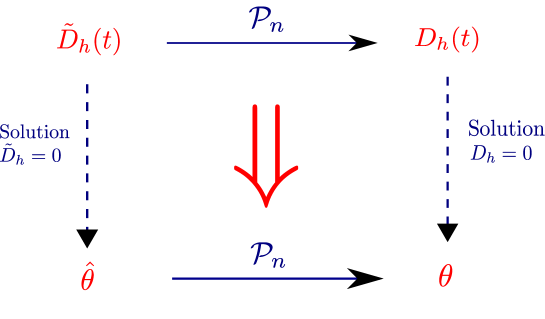
Figure 1: Illustration of the deviations’ control. ${\cal P}_{n}$ represent the probability convergence.

Properties of the function $D_{h}(\cdot)$ allow us to prove that $\theta$ is the unique solution of $D_{h}(\cdot)=0$. We also notice that $|\hat{f}^{h}({x_{0}})-f({x_{0}})|\leq\|\hat{\theta}-\theta\|_{1}$. The idea (presented in Figure 1) is to deduce the exponential inequality for $\|\hat{\theta}-\theta\|_{1}$ from the exponential inequality for $\sup_{t}\big{|}\tilde{D}_{h}(t)-D_{h}(t)\big{|}$. As we mentioned above, we notice that $\sup_{t}\big{|}\tilde{D}_{h}(t)-D_{h}(t)\big{|}$ can be viewed as the supremum of an empirical process.

Now, classical arguments in probability tools can be used. To control $\sup_{t}\big{|}\tilde{D}_{h}(t)-D_{h}(t)\big{|}$, we could used standard tools developed by Talagrand [1996a, 1996b], [27] or [3]. But the obtained exponential inequalities (like (1.6)) contain unknown constants or require the knowledge of an expectation’s bound of $\sup_{t}\big{|}\tilde{D}_{h}(t)-D_{h}(t)\big{|}$. To obtain this bound, we can use the maximal inequalities developed by [40] (Chapter 2, Section 2.2) for sub-gaussian processes. But here again, there are universal constants (and unknown) in the bound of the expectation. [28] (Chapter 6) gives exponential inequalities for $\sup_{t}\big{|}\tilde{D}_{h}(t)-D_{h}(t)\big{|}$ without the expectation, but some constants are very big in our case. In this paper, we choose to apply standard chaining argument and Bernstein’s inequality (cf. (7.8)) directly on $\sup_{t}\big{|}\tilde{D}_{h}(t)-D_{h}(t)\big{|}$ (cf. Proof of Lemma 3). That allows us to have constants smaller the ones cited in the papers above.

Perspectives.

• We think that conditions on the noise densities could be reduced. We could consider the densities not necessary monotonically on ${\mathbb{R}}_{+}$, only the symmetric assumption seems necessary.

• A possible perspective of this work is the study of estimating anisotropic functions. Indeed, the method developed by [20], [21] and Goldenshluger and Lepski [2008, 2009] are based on the linear properties and the machinery considered in those works can not adapt straightforwardly to nonlinear estimators.

• Another perspective is to prove an oracle inequality for the family of $\rho$-LPA estimators indexed by the bandwidth with the integrated risk. It could be interesting to introduce some criterion for choosing the optimal contrast function.

• Finally, we should also study the heteroscedastic model (1.1) with a degenerate design when the design density is vanishing or exploding.

This paper is organized as follows. We present exponential inequalities in Section 2, in order to control deviations of $\rho$-LPA estimator. In Section 3, we present the results concerning minimax estimation and Section 4 is devoted to the adaptive estimation. An application of $\rho$-LPA estimator with Huber function is proposed in Section 5. The proofs of the main results (exponential inequalities and upper bounds) are given in Section 6, technical lemmas are postponed to the appendix.

2 Exponential inequality for $\rho$-LPA estimator

Construction.

To construct our estimator, we use the so-called local polynomial approach (LPA) which consists in the following. Let

$$V_{x_{0}}(h)=\bigotimes_{j=1}^{d}\big{[}y_{j}-h/2,y_{j}+h/2\big{]}\cap[0,1]^{d},$$

be a neighborhood around $x_{0}$ of width $h\in(0,1)$. Fix $b>0$ (without loss of generality we will assume that $b$ is an integer), let

$${\cal S}_{b}=\{p=(p_{1},\ldots,p_{d})\in{\mathbb{N}}^{d}:\;0\leq|p|\leq b,\>|p|=p_{1}+\ldots+p_{d}\},$$

and we denote $N_{b}$ the cardinal of ${\cal S}_{b}$. Let $U(z),z\in{\mathbb{R}}^{d}$ be the $N_{b}$-dimensional vector of monomials of the following type (the sign $\top$ below denotes the transposition):

$$U^{\top}(z)=\left(\prod_{j=1}^{d}z_{j}^{p_{j}},\;\;p\in{\cal S}_{b}\right).$$ (2.1)

For any $t^{\top}=\big{(}t_{p_{1},\ldots,p_{d}}\in{\mathbb{R}}\>:\>p\in{\cal S}_{b}\big{)}\in{\mathbb{R}}^{N_{b}}$, we define the local polynomial in a neighborhood of $x_{0}$ as for any $x\in[0,1]^{d}$

$$f_{t}(x) = t^{\top}U\left(\frac{x-{x_{0}}}{h}\right){\mathbb{I}}_{V_{x_{0}}(h)}(x)=\sum_{p\in{\cal S}_{b}}t_{p}\>\left(\frac{x-{x_{0}}}{h}\right)^{p}{\mathbb{I}}_{V_{x_{0}}(h)}(x),$$ (2.2)

where $z^{p}=z_{1}^{p_{1}}\cdots z_{d}^{p_{d}}$ for $z=(z_{1},\dots,z_{d})$ and ${\mathbb{I}}$ denotes the indicator function. For any $M>0$, introduce the following subset of ${\mathbb{R}}^{N_{b}}$

$$\Theta\big{(}M\big{)}=\left\{t\in{\mathbb{R}}^{N_{b}}:\;\;\|t\|_{1}\leq M\right\},$$ (2.3)

where $\|\cdot\|_{1}$ is $\ell_{1}$-norm on ${\mathbb{R}}^{N_{b}}$. We notice that for any $t\in\Theta(M)$, $\|f_{t}\|_{\infty}\leq M$ where $\|\cdot\|_{\infty}$ is the sup-norm on $[0,1]^{d}$.

The function $\rho$ is called contrast function if it has the following properties.

Assumption 1.

1. $\rho:{\mathbb{R}}\rightarrow{\mathbb{R}}_{+}$ is symmetric, convex and $\rho(0)=0$,

2. the derivative $\rho^{\prime}$ is $1$-Lipschitz on ${\mathbb{R}}$ and bounded: $\dot{\rho}_{\infty}=\|\rho^{\prime}\|_{\infty}<\infty$,

3. the second derivative $\rho^{\prime\prime}$ is defined almost everywhere and there exist $L_{\rho}>0$ and $\alpha>0$ such that

   $$\sup_{i=\overline{1,n}}\int_{\mathbb{R}}\big{|}\rho^{\prime\prime}(z+u)-\rho^{\prime\prime}(z+v)\big{|}\>g_{i}(z)\>dz\leq L_{\rho}\>|u-v|^{\alpha},\quad\forall u,v\in{\mathbb{R}}.$$

   where $\overline{1,n}=1,\ldots,n$.

A well-known example of a contrast function $\rho$ satisfying Assumption 1 above is the Huber function (cf. [16]) presented in Section 5.

Let $K$ be a kernel function, i.e. a positive function with a compact support included in $[-1/2,1/2]^{d}$ such that $K_{\infty}:=\|K\|_{\infty}<\infty$ and $\int_{\mathbb{R}}K(z)dz=1$. We will construct the $\rho$-LPA estimator for $f({x_{0}})$ using local $\rho$-criterion which is defined as follows:

$$\tilde{\pi}_{h}(t)=\tilde{\pi}_{h}\big{(}t,Z^{(n)}\big{)}=\frac{1}{nh^{d}}\sum_{i=1}^{n}\rho\big{(}Y_{i}-f_{t}(X_{i})\big{)}\>K\left(\frac{X_{i}-{x_{0}}}{h}\right).$$ (2.4)

Let $\hat{\theta}(h)$ be the solution of the following minimization problem:

$$\hat{\theta}(h)=\arg\min_{t\in\Theta(M)}\tilde{\pi}_{h}(t).$$ (2.5)

The $\rho$-LPA estimator $\hat{f}^{h}({x_{0}})$ of $f({x_{0}})$ is defined as $\hat{f}^{h}({x_{0}})=\hat{\theta}_{0,...,0}(h)$. We notice that this local approach can be considered as the estimation for successive derivatives of the function $f$. However in the present paper, we focus on the estimation of $f({x_{0}})$.

Exponential inequality.

Later on, we will only consider values of $h\in[n^{-1/d},1]$. Put $\theta=\theta(f,x_{0},h)=\big{\{}\theta_{p}:\;p\in{\cal S}_{b}\big{\}}$, where $\theta_{0}=\theta_{0,...,0}=f({x_{0}})$ and

$$\forall p\in{\cal S}_{b}\>:\>p\neq 0,\quad\theta_{p}=\displaystyle\frac{\partial^{|p|}f({x_{0}})}{\partial y_{1}^{p_{1}}\cdots\partial y_{d}^{p_{d}}}\frac{h^{|p|}}{p_{1}!...p_{d}!}.$$ (2.6)

Here, we do not assume the existence of partial derivatives of $f$. To define $\theta$ properly, the following agreement will be used in the sequel: if the function $f$ and the vector ${p}$  are such that $\partial^{|p|}f$ does not exist, we put $\theta_{p}=0$.

Set ${\cal B}\big{(}\theta,z\big{)}=\left\{t\in\Theta(M):\>\|t-\theta\|_{2}\leq z\right\}$ the Euclidean ball with radius $z$ and center $\theta$ and define the event for any $h,z>0$

$$G_{z}^{h} = \big{\{}\hat{\theta}(h)\in{\cal B}\big{(}\theta,z\big{)}\big{\}},\quad$$ (2.7)

where $\hat{\theta}(h)$ is given by (2.5). Let

$$\Sigma=2+2\sum_{l=1}^{\infty}d^{2}10^{2l-1}\>\exp\left\{-\frac{18\>10^{l}}{\pi^{4}\>l^{4}}\frac{(8K_{\infty})^{-1}}{K_{\infty}+1/3}\right\},$$ (2.8)

be some finite constants and let the constant $\lambda$ be the smallest eigenvalue of matrix

$$\int_{[-1/2,1/2]^{d}}U(x)\>U^{\top}(x)\>K(x)\>dx.$$

[38] (Lemma 1.4) showed that $\lambda$ is positive, on the hand the last matrix is strictly positive definite. Finally, put

$$c\big{(}\rho,(g_{i})_{i}\big{)}=\inf_{i=1,\ldots,n}\int_{\mathbb{R}}\rho^{\prime\prime}(z)\>g_{i}(z)\>dz,$$ (2.9)

and define the set of sequences of symmetric densities which are monotonically on ${\mathbb{R}}_{+}$

$${\cal G}_{\rho}^{(c)}=\left\{(g_{i})_{i}\>:\>c\big{(}\rho,(g_{i})_{i}\big{)}\geq c\right\},\quad c>0.$$ (2.10)

Denote for all $a,b\in{\mathbb{R}},\>a\vee b=\max(a,b)$. The next proposition is the milestone for all results proved in the paper.

Proposition 1.

Let $\rho$ be a contrast function and let $c>0$. Then, for any $n\in{\mathbb{N}}^{*}$, $(g_{i})_{i}\in{\cal G}_{\rho}^{(c)}$, $h>n^{-1/d}$, $M>0$, $x_{0}\in[0,1]^{d}$ and any $f$ such that $\|\theta(f,x_{0},h)\|_{1}\leq M$, we have for any $\varepsilon\geq\frac{4N_{b}}{{c\lambda}}\big{(}1\vee b_{h}\>\sqrt{nh^{d}}\big{)}$

$$\mathbb{P}_{f}\left(\sqrt{nh^{d}}\big{|}\hat{f}^{h}({x_{0}})-f({x_{0}})\big{|}\geq\varepsilon,\>G_{\delta}^{h}\right)$$

$$\quad\leq N_{b}\varSigma\exp\left\{-\frac{\left(\frac{c\lambda}{{2N_{b}}}\>\varepsilon-\big{(}1\vee b_{h}\>\sqrt{nh^{d}}\big{)}\right)^{2}}{8K_{\infty}^{2}(1\vee\dot{\rho}_{\infty}^{2})+\frac{4\>K_{\infty}}{3{N_{b}}}\>(1\vee{\dot{\rho}_{\infty}})\frac{c\lambda\>\varepsilon}{\sqrt{nh^{d}}}}\right\}.$$ (2.11)

The proof of this proposition is given in Section 6.

Remark 1.

The control of the deviations of $\hat{f}^{h}$ is realized under the event $G_{\delta}^{h}$ that the estimator $\hat{\theta}(h)$ is contained in a ball centered at $\theta$ whereas its radius does not depend on $n$, else it could change the rate of convergence. In Section 6 we give an exponential inequality to control the probability of the complementary of $G_{\delta}^{h}$ (cf. Lemma 4).

Remark 2.

In the minimax case, the knowledge of constants in (1) is not required. However for adaptation, the constant $c$ is involved in the construction of adaptive estimator. This restricted the consideration of the noise densities which satisfy (2.10). We notice that this problem is simplified to the calibration of an alone constant with a dataset.

3 Minimax Results on $\mathbb{H}_{d}({\beta},L,M)$

In this section, we present several results concerning maximal and minimax risks on $\mathbb{H}_{d}({\beta},L,M)$. We propose the estimator which bound the maximal risk on this class of functions without restriction imposed on these parameters.

Preliminaries.

Definition 1.

Fix $\beta>0$, $L>0$, $M>0$ and let $\lfloor\beta\rfloor$ be the largest integer strictly smaller than $\beta$. The isotropic Hölder class $\mathbb{H}_{d}({\beta},L,M)$ is the set of functions $f:[0,1]^{d}\rightarrow{\mathbb{R}}$ admitting on $[0,1]^{d}$ all partial derivatives of order $\lfloor\beta\rfloor$ and such that for any $x,y\in[0,1]^{d}$

$$\left|\frac{\partial^{|p|}f(x)}{\partial x_{1}^{p_{1}}\cdots\partial x_{d}^{p_{d}}}-\frac{\partial^{|p|}f({y})}{\partial y_{1}^{p_{1}}\cdots\partial y_{d}^{p_{d}}}\right| \leq L\big{[}\|x-{y}\|_{1}\big{]}^{\beta-\lfloor\beta\rfloor},\quad\forall\;\big{|}{p}\big{|}=\lfloor\beta\rfloor,$$

$$\sum_{p\in{\cal S}_{\lfloor\beta\rfloor}}\sup_{x\in[0,1]^{d}}\left|\frac{\partial^{|p|}f(x)}{\partial x_{1}^{p_{1}}\cdots\partial x_{d}^{p_{d}}}\right| \leq M.$$

where $x_{j}$ and $y_{j}$ are the $j^{th}$ components of $x$ and $y$.

Let $\mathbb{E}_{f}=\mathbb{E}^{n}_{f}$ be the mathematical expectation with respect to the probability law ${\mathbb{P}}_{f}$ of the observation $Z^{(n)}$ satisfying (1.1). Firstly, we define the maximal risk on $\mathbb{H}_{d}({\beta},L,M)$ corresponding to the estimation of the function $f$ at a given point $x_{0}\in[0,1]^{d}$.

Let $\tilde{f}_{n}$ be an arbitrary estimator built from the observation $Z^{(n)}$. For any $r$ let

$$R_{n,r}\big{[}\tilde{f}_{n},\mathbb{H}_{d}({\beta},L,M)\big{]}=\sup_{f\in\mathbb{H}_{d}({\beta},L,M)}\mathbb{E}_{f}\big{|}\tilde{f}_{n}({x_{0}})-f({x_{0}})\big{|}^{r}.$$ (3.1)

This quantity is called maximal risk of the estimator $\tilde{f}_{n}$ on $\mathbb{H}_{d}({\beta},L,M)$ and the minimax risk on $\mathbb{H}_{d}({\beta},L,M)$ is defined as

$$R_{n,r}\big{[}\mathbb{H}_{d}({\beta},L,M)\big{]}=\inf_{\tilde{f}}R_{n,r}\big{[}\tilde{f},\mathbb{H}_{d}({\beta},L,M)\big{]},$$ (3.2)

where the infimum is taken over the set of all estimators.

Definition 2.

The normalizing sequence $\psi_{n}$ is called minimax rate of convergence and the estimator $\hat{f}$ is called minimax (asymptotically minimax) if

$$\liminf_{n\to\infty}\psi^{-r}_{n}\>R_{n,r}\big{[}\hat{f},\mathbb{H}_{d}({\beta},L,M)\big{]} > 0,$$ (3.3)

$$\limsup_{n\to\infty}\psi^{-r}_{n}\>R_{n,r}\big{[}\hat{f},\mathbb{H}_{d}({\beta},L,M)\big{]} < \infty.$$ (3.4)

Upper bound for maximal risk.

Let the minimizer of the bias/variance trade-off (1.5) be given by

$$\bar{h}=(L^{2}n)^{-\frac{1}{2\beta+d}}.$$ (3.5)

The next theorem shows how to construct the estimator based on locally parametric approach which achieves the following rate of convergence in the model (1.1)

$$\varphi_{n}({\beta})=n^{-\frac{{\beta}}{2{\beta}+d}}.$$ (3.6)

Let $\hat{f}^{\bar{h}}({x_{0}})=\hat{\theta}_{0,\ldots,0}\big{(}\bar{h}\big{)}$ be given by (2.3), (2.4) and (2.5) with $h=\bar{h}$ and $b=\lfloor\beta\rfloor$.

Theorem 1.

Let $\beta>0$, $L>0$, $M>0$, $x_{0}\in[0,1]^{d}$, $c>0$ and let $\rho$ be a fixed contrast function. Then for any $(g_{i})_{i}\in{\cal G}_{\rho}^{(c)}$

$$\limsup_{n\to\infty}\>\varphi_{n}^{-r}(\beta)\>R_{n,r}\Big{[}\hat{f}^{\bar{h}}({x_{0}}),\mathbb{H}_{d}({\beta},L,M)\Big{]}<\infty,\quad\forall r\geq 1.$$

This theorem will be deduced from Proposition 1 and the proof is given in Section 6.2.

Remark 3.

[34] showed lower bounds (3.3) for rate $n^{-\frac{\beta}{2\beta+d}}$ with the following assumption on Kullback distance on the noise density $g$, i.e. it exists $v_{0}>0$ such that

$$\int g(u)\>\ln\frac{g(u)}{g(u+v)}\>du\leq o\big{(}v^{2}\big{)},\quad\forall v\>:\>|v|\leq v_{0}.$$

We notice that Gaussian and Cauchy densities verify this assumption (cf. also [38] Chapter 2). In this case, we conclude that $\hat{f}^{\bar{h}}$ is minimax and $\varphi_{n}(\beta)$ is the minimax rate on $\mathbb{H}_{d}({\beta},L,M)$.

4 Bandwidth Selection of $\rho$-LPA Estimator

This section is devoted to the adaptive estimation over the collection of classes $\Big{\{}\mathbb{H}_{d}(\beta,L,M)\Big{\}}_{\beta,L}$. Here we suppose $M$ known, as we mentioned in the introduction, the parameter $M$ could be estimated and used with a “Plug-in” method (cf. [14]). We will not impose any restriction on the possible value of $L$, but we will assume that $\beta\in(0,b]$, where $b$ as previously, is an arbitrary chosen integer.

We start by remarking that there is not optimally adaptive estimator. Well-known disadvantage of maximal approach is the dependence of the estimator on the smoothness parameters describing the functional class on which the maximal risk is determined (cf. (3.1)). In particular, $\bar{h}_{n}({\beta},L)$, optimally chosen in view of (1.5), depends explicitly on ${\beta}$ and $L$. To overcome this drawback, a maximal adaptive approach has been proposed by [23] for pointwise estimation. The first question arising in the adaptation (reduced to the problem at hand) can be formulated as follows.

Does there exist an estimator which would be minimax on $\mathbb{H}({\beta},L,M)$ simultaneously for all values of ${\beta}$ and $L$ belonging to some given set $\mathfrak{B}\subseteq\big{[}{\mathbb{R}}_{+}\setminus{0}\big{]}\times\big{[}{\mathbb{R}}_{+}\setminus{0}\big{]}$ ?

For integrated risks, the answer is positive (cf. [24], [8], [26], [11] and [17]). For the estimation of the function at a given point, it is typical that the price to pay is not null (cf. [23], [4], [26], [39], [21], [30], [7]). Mostly, the price to pay is a power of $(b-\beta)\ln n$ for pointwise estimation.

Let $\Psi=\left\{\psi_{n}(\beta)\right\}_{\beta\in(0,b]}$ be a given family of normalizations.

Definition 3.

The family $\Psi$ is called admissible if there exists an estimator $\hat{f}_{n}$ such that for some $L,M>0$

$$\limsup_{n\rightarrow\infty}\psi^{-r}_{n}(\beta)\;R_{n,r}\big{(}\hat{f}_{n},\mathbb{H}_{d}(\beta,L,M)\big{)}<\infty,\;\;\forall\beta\in(0,b].$$ (4.1)

The estimator $\hat{f}_{n}$ satisfying (4.1) is called $\Psi$-attainable. The estimator $\hat{f}_{n}$ is called $\Psi$-adaptive if (4.1) holds for any $L>0$.

[23] showed that the family of rates $\left\{\varphi_{n}(\beta)\right\}_{\beta\in(0,b]}$, defined in (3.6), is not admissible in the white noise model. With other tools, [4] extend this result for density estimation and nonparametric Gaussian regression. It means that there is no-estimator which would be minimax simultaneously for several values of parameter $\beta$, for pointwise estimation, even if $L$ is supposed to be fixed. This result does not require any restriction on $\beta$ as well.

Now, we need to find another family of normalizations for maximal risk which would be attainable and, moreover, optimal in view of some criterion of optimality. Let $\Phi$ be the following family of normalizations, for any $\beta\in(0,b]$

$$\phi_{n}(\beta)=\left(\frac{\varrho_{n}(\beta)}{n}\right)^{\frac{\beta}{2\beta+d}},\quad\varrho_{n}(\beta)=1+\frac{2(b-\beta)}{(2\beta+d)(2b+d)}\ln n.$$ (4.2)

We notice that $\phi_{n}(b)=\varphi_{n}(b)$ and for $n$ large enough $\varrho_{n}(\beta)\sim{(b-\beta)\ln n}$ for any $\beta\neq b$. It is possible to show that this family $\Phi$ is adaptive optimal using the most recent criterion developed by [21] used for the white noise model and used by [7] for the multiplicative uniform regression. On the other hand, the so-called price to pay for adaptation $\varrho_{n}(\beta)$ could be considered as optimal.

Construction of $\Phi$-adaptive estimator.

We begin by stating that the construction of our estimation procedure is decomposed in several steps. First, we determine the family of $\rho$-LPA estimators. Next, based on Lepski’s method, we propose a data-driven selection from this family.

Let $\rho$ be a fixed contrast function. In the model (1.1), we recall that the sequence of densities $(g_{i})_{i}$ is “unknown” for the statistician. We take $\hat{f}^{h}$ the estimator given by (2.3), (2.4) and (2.5), so the family of $\rho$-LPA estimators $\hat{{\cal F}}$ is defined now as follows. Put

$$h_{\min}=(\ln n)^{2/d}n^{-1/d},\quad h_{\max}=n^{-\frac{1}{2b+d}},$$ (4.3)

and

$$h_{k}=2^{-k}h_{\max},\;\;k=\overline{0,\mathbf{k}_{n}}:=0,\ldots,\mathbf{k}_{n},$$

where $\mathbf{k}_{n}$ is the largest integer such that $\displaystyle h_{\mathbf{k}_{n}}\geq h_{\min}$. Set

$$\hat{{\cal F}}=\left\{\hat{f}^{(k)}({x_{0}})=\hat{\theta}_{0,\ldots,0}(h_{k}),\;\;k=\overline{0,\mathbf{k}_{n}}\right\}.$$ (4.4)

We put $\hat{f}^{*}({x_{0}})=\hat{f}^{(\hat{k})}({x_{0}})$, where $\hat{f}^{(\hat{k})}({x_{0}})$ is selected from $\hat{{\cal F}}$ in accordance with the rule:

$$\hat{k}=\inf\left\{k=\overline{0,\mathbf{k}_{n}}:\;\;\big{|}\hat{f}^{(k)}({x_{0}})-\hat{f}^{(l)}({x_{0}})\big{|}\leq CS_{n}\big{(}l\big{)},\;\;l=\overline{k+1,\mathbf{k}_{n}}\right\}.$$ (4.5)

Here we have used the following notations. Let $c>0$ be fixed and

$$C = {\frac{4N_{b}}{c\lambda}}\left(1+2\>K_{\infty}\>(1\vee\dot{\rho}_{\infty})\sqrt{rd}\right),$$ (4.6)

$$S_{n}(l) = \left[\frac{1+l\ln 2}{n\big{(}h_{l}\big{)}^{d}}\right]^{1/2},\quad l=\overline{0,\mathbf{k}_{n}},$$

where $r\geq 1$ is the power of the risk and $c$ is defined in (2.9), ${\dot{\rho}_{\infty}}$ and $K_{\infty}$ are respectively bounds of $\rho^{\prime}(\cdot)$ and $K(\cdot)$, and the positive constant $\lambda$ is the smallest eigenvalue of the matrix $\int_{[-0.5,0.5]^{d}}U(x)\>U^{\top}(x)\>K(x)\>dx$. We will see that this matrix is strictly positive definite (cf. Lemma 1).

Main Result.

The next theorem is the main result of this paper. It allows us to guarantee a good performance of our adaptive $\rho$-LPA estimator $\hat{f}^{*}$.

Theorem 2.

Let $b>0,M>0$ and $\rho$ be a fixed contrast function. Then, for any $(g_{i})_{i}\in{\cal G}_{\rho}^{(c)}$, $\beta\in(0,b]$, $L>0$ and $r\geq 1$

$$\limsup_{n\to\infty}\phi_{n}^{-r}(\beta)\;R_{n,r}\Big{[}\hat{f}^{*}({x_{0}}),\mathbb{H}_{d}({\beta},L,M)\Big{]}<\infty.$$

The proof (given in Section 6.3) is based on the scheme due to [22].

Remark 4.

The assertion of the theorem means that the proposed estimator $\hat{f}^{*}({x_{0}})$ is $\Phi$-adaptive in the model (1.1) (cf. Definition 3). It implies in particular that the family of normalizations $\Phi$ is admissible.

Remark 5.

In the present paper, we do not give the explicit expression of the constant in the upper bound of the risk with the proof given in this paper. But it is possible to solve this problem. In the proof of Lepski’s method, we notice that the upper bound polynomially depends on the parameter $C$ and it is important to minimize this constant. We see that this constant depends on the contrast function $\rho$ and it is easy to see that minimizing $C=C(\rho)$ can be viewed as minimizing the following Huber variance (cf. [15] Page 74)

$$\sigma^{2}_{\rho}=\frac{\int\big{(}\rho^{\prime}\big{)}^{2}\>dg}{\left(\int\rho^{\prime\prime}\>dg\right)^{2}}\rightarrow\min_{\rho},$$

where $g$ is the noise density in the homeoscedastic model.

Remark 6.

The limitation concerning the consideration of isotropic classes of functions is due to the use of Lepski’s procedure. It seems that to be able to treat the adaptation over the scale of anisotropic classes (i.e. $d$-dimensional functions with different regularities $\beta$ for each variable). Another scheme should be applied as in [25], [20], [21] and [9]. As we have mentioned above, these latter procedures cannot be used with $\rho$-LPA estimators, and for the model (1.1) this problem is still open.

5 Application: Huber function

Consider the model (1.1), with following additional assumptions.

$$g_{i}(\cdot)=g(\cdot/\sigma_{i})/\sigma_{i},\quad i=1,...,n,$$ (5.1)

where the density $g$ is symmetric and monotonically on ${\mathbb{R}}_{+}$. $(\sigma_{i})_{i}$ is a sequence of real values such that for any $i,\>0<\sigma_{\min}\leq\sigma_{i}<\infty$ where $\sigma_{\min}$ is known. The model (1.1) with (5.1) can be written as

$$Y_{i}=f(X_{i})+\sigma_{i}\>\xi_{i},\quad i=1,...,n,$$ (5.2)

where $(\xi_{i})$ are i.i.d. with the density $g$.

Let

$$\rho_{\gamma}(z)=\gamma(z-0.5\>\gamma)\>{\mathbb{I}}_{|z|>\gamma}+0.5\>z^{2}\>{\mathbb{I}}_{|z|\leq\gamma},\>z\in{\mathbb{R}},\>\gamma\geq 0.$$ (5.3)

the Huber function ([16]). We construct the $\rho_{\gamma}$-LPA estimator from (2.3), (2.4) and (2.5). The function $\rho_{\gamma}$ is a contrast function verifying Assumption 1. Recall that the constant $c=c\big{(}\rho_{\gamma},(g_{i})_{i}\big{)}$ defined in (2.9) must be positive. We notice that the second derivative can be written as $\rho_{\gamma}^{\prime\prime}(\cdot)={\mathbb{I}}_{[-\gamma,\gamma]}(\cdot)$ and that

$$c\big{(}\rho_{\gamma},(g_{i})_{i}\big{)}\geq c_{\gamma}:=2\int_{0}^{\gamma\sigma_{\min}}g(z)dz.$$

We formulate the following assertion: for any $\sigma_{\min}>0$ and any $g$ a symmetric density and monotonically on ${\mathbb{R}}_{+}$, there exists a constant $\gamma_{0}>0$ such that for any $\gamma\geq\gamma_{0},\>c_{\gamma}>0$.

We propose the adaptive $\rho_{\gamma_{0}}$-LPA estimator $\hat{f}^{*}_{\gamma_{0}}({x_{0}})$ selected with the data-driven selection proposed in Section 4 with the constant

$$C={\frac{2N_{b}}{\lambda\int_{0}^{\gamma_{0}\sigma_{\min}}g(z)dz}}\left(1+2\>K_{\infty}\>(1\vee\gamma_{0})\sqrt{rd}\right).$$

The next result is a direct consequence of Theorem 2.

Corollary 1.

Let $b>0$, $M>0$ be some fixed constants and consider the model (5.2). Then, for any $(g_{i})_{i}\in{\cal G}_{\rho_{\gamma_{0}}}^{(c_{\gamma_{0}})}$, $\beta\in(0,b]$, $L>0$ and $r\geq 1$

$$\limsup_{n\to\infty}\phi_{n}^{-r}(\beta)R_{n,r}\Big{[}\hat{f}^{*}_{\gamma_{0}}({x_{0}}),\mathbb{H}_{d}({\beta},L,M)\Big{]}<\infty.$$

Remark 7.

We notice that the threshold parameter $C$ explicitly depends on the minoration $\sigma_{\min}$ of the noises variances $(\sigma_{i})_{i}$. Contrary to linear estimators (C polynomially depends on $(\sigma_{i})_{i}$), we can see that the influence of $(\sigma_{i})_{i}$ is very limited for $\rho$-LPA estimators.

Remark 8.

Corollary 1 only guarantees that asymptotically for any $\gamma\geq\gamma_{0}$, $\rho_{\gamma}$-LPA estimators have the same performance. In the future, an important question to adress is: how one can choose the parameter $\gamma$? In theory, there is yet no criterion for choosing an optimal $\gamma$, but we can make the following remarks. If $\gamma=\infty$, then the ${\rho}_{\infty}$-LPA estimator is the least square estimator (sensitive to extreme values of the noise) and if $\gamma=0$ then the $\rho_{0}$-LPA estimator becomes the median estimator (robust estimator). It is well-known that least squares estimator and median estimator respectively suffer from undersmoothing and oversmoothing. This phenomenon is highlighted by [30]. We believe that a better choice of parameter $\gamma$ should give a “semi-robust” estimator. Locally this could reduce the above mentioned issue. In practice, it will be interesting to select the parameter $\gamma$ as a measurable function of observations which adapts to extreme values of the noise. This problem is related to the estimation of the noise variance and to the minimization of the Huber variance (cf. [15] Page 74).

6 Proofs of Main Results: Exponential inequalies and Upper Bounds

6.1 Proof of Proposition 1

Notations.

Recall that ${\cal S}_{b}=\big{\{}q\in{\mathbb{N}}^{d}\>:\>|q|\leq b,\>|q|=q_{1}+\ldots+q_{d}\big{\}}$ and $N_{b}$ its cardinal. We consider the partial derivative of the local $\rho$-criterion

$$\tilde{D}_{h}(\cdot)=\left(\frac{\partial}{\partial t_{p}}\>\tilde{\pi}_{h}(\cdot)\right)_{p\in{\cal S}_{b}}^{\top},$$ (6.1)

where $\tilde{\pi}_{h}(\cdot)$ is the local $\rho$-criterion defined in (2.4). Let also

$${\cal E}_{h}(\cdot)=\mathbb{E}_{f}\left[\tilde{D}_{h}(\cdot)\right]\quad\text{and}\quad D_{h}(\cdot)=\mathbb{E}_{f_{\theta}}\big{[}\tilde{D}_{h}(\cdot)\big{]},$$ (6.2)

where $f_{\theta}$ is the Taylor polynomial defined in (2.6), $\mathbb{E}_{f_{\theta}}=\mathbb{E}_{f_{\theta}}^{n}$ be the mathematical expectation with respect to the probability law ${\mathbb{P}}_{f_{\theta}}$ of the “parametric” observations $(X_{i},{\cal Y}_{i})_{i=1,...,n}$ (cf. (1.4)) and $\mathbb{E}_{f}=\mathbb{E}_{f}^{n}$ be the mathematical expectation with respect to the probability law ${\mathbb{P}}_{f}$ of the observation $Z^{(n)}$.

We call the Jacobian matrix $J_{D}$ of $D_{h}$ such that

$$\big{(}J_{D}(\cdot)\big{)}_{p,q\in{\cal S}_{b}}:=\left(\frac{\partial}{\partial t_{q}}D_{h}^{p}(\cdot)\right)_{p,q\in{\cal S}_{b}}=\left(\mathbb{E}_{f_{\theta}}\frac{\partial^{2}}{\partial t_{p}\partial t_{q}}\>\tilde{\pi}_{h}(\cdot)\right)_{p,q\in{\cal S}_{b}},$$ (6.3)

where $D_{h}^{p}(\cdot)$ is the $p^{th}$ component of $D_{h}(\cdot)$.

Auxiliary lemmas.

We give the following lemma concerning the deterministic criterion $D_{h}$ defined in (6.2). Denote $\|\cdot\|_{2}$ the $\ell_{2}$-norm on ${\mathbb{R}}^{N_{b}}$.

Lemma 1.

Let $\rho$ be a contrast function, for any $(g_{i})_{i}\in{\cal G}_{\rho}^{(c)}$ we have the following assertions:

1. the matrix $J_{D}(\theta)$ is strictly positive definite and $\theta$ is the unique solution of the equation $D_{h}(\cdot)=(0,...,0)$ on $\Theta(M)$,

2. there exists $\delta>0$ which only depends on the contrast function $\rho$ such that for any $\tilde{\theta}\in{\cal B}(\theta,\delta)$, we have

   $$\|\tilde{\theta}-\theta\|_{2}\leq{\frac{2}{c\lambda}}\inf_{h>0}\left\|D_{h}\big{(}\tilde{\theta}\big{)}-D_{h}(\theta)\right\|_{2}.$$

Recall that $b_{h}=\sup_{x\in V_{x_{0}}(h)}\big{|}f_{\theta}(x)-f(x)\big{|}$ corresponds to the approximation error (bias) and denote ${\cal E}_{h}^{p}(\cdot)$ the $p^{th}$ component of ${\cal E}_{h}(\cdot)$. Let us give a lemma which allows us to control the bias term.

Lemma 2.

For any contrast function $\rho$, $h>n^{-1/d}$ and any $f$ such that $\|\theta\|_{1}\leq M$, we have

$$\max_{p\in{\cal S}_{b}}\sup_{t\in\Theta(M)}\big{|}{\cal E}_{h}^{p}(t)-D_{h}^{p}(t)\big{|}\leq b_{h}.$$

The next result allows us to control deviations of partial derivatives of $\rho$-criterion $\tilde{D}_{h}$ defined in (6.1).

Lemma 3.

For any contrast function $\rho$, any $f$ such that $\|\theta\|_{1}\leq M$ and any $h>n^{-1/d}$, we have for any $z\geq 2\big{(}1\vee b_{h}\>\sqrt{nh^{d}}\big{)}$

$$\max_{p\in{\cal S}_{b}}{\mathbb{P}}_{f}\left(\sqrt{nh^{d}}\sup_{t\in\Theta(M)}\left|\tilde{D}_{h}^{p}(t)-{\cal E}_{h}^{p}(t)\right|\geq z\right)$$

$$\quad\leq\varSigma\exp\left\{-\frac{\left(z-b_{h}\>\sqrt{nh^{d}}\right)^{2}}{8K_{\infty}^{2}\>(1\vee\dot{\rho}_{\infty}^{2})+\frac{4K_{\infty}}{3\sqrt{nh^{d}}}\>(1\vee{\dot{\rho}_{\infty}})z}\right\}.$$

As we mentioned above, the partial derivatives $\big{(}\tilde{D}_{h}^{p}(\cdot)\big{)}_{p}$ can be considered as empirical processes. Thus the proof (given in Appendix) is based on a chaining argument and Bernstein’s inequality (cf. (7.8)). In particular, it is required that the derivative $\rho^{\prime}$ of the contrast function is bounded and Lipschitz.

Denote by $\bar{G}_{\delta}^{h}$ the complementary of $G_{\delta}^{h}$ (defined in (2.7)) where the radius $\delta$ is defined in Lemma 1 and let $\varkappa_{\delta}=\inf_{t\in\Theta(M)\backslash{\cal B}(\theta,\delta)}\|D_{h}(t)\|_{2}/2$ be a positive constant. The next lemma allows us to control the probability of the event that “the $\rho$-LPA estimator does not belong to the ball centered on $\theta$ with radius $\delta$”.

Lemma 4.

For any contrast function $\rho$, $f\in\mathbb{H}_{d}(\beta,L,M)$, $\delta>0$ and $n\in{\mathbb{N}}^{*}$ such that

$$\frac{\varkappa_{\delta}}{\sqrt{N_{b}}}\geq 2\sup_{h\in[h_{\min},h_{\max}]}\big{(}1\vee b_{h}\sqrt{nh^{d}}\big{)},$$

we have

$${\mathbb{P}}_{f}\left[{\bar{G}_{\delta}^{h}}\right]\leq N_{b}\varSigma\>\exp\left\{-\frac{nh^{d}\left(\varkappa_{\delta}/2\sqrt{N_{b}}\right)^{2}}{8K_{\infty}^{2}\>(1\vee\dot{\rho}_{\infty}^{2})+\frac{4\varkappa_{\delta}}{3\sqrt{N_{b}}}\>K_{\infty}\>(1\vee{\dot{\rho}_{\infty}})}\right\}.$$

Proofs of those lemmas are given in Appendix.

Proof of Proposition 1.

Definitions of $\hat{\theta}(h)$ and $\theta=\theta(f,x_{0},h)$ imply that for any $\varepsilon\geq\frac{4N_{b}}{c\lambda}\big{(}1\vee b_{h}\sqrt{nh^{d}}\big{)}$

$$\mathbb{P}_{f}\left(\sqrt{nh^{d}}\big{|}\hat{f}^{h}({x_{0}})-f({x_{0}})\big{|}\geq\varepsilon,\>G_{\delta}^{h}\right) \leq \mathbb{P}_{f}\left(\sqrt{nh^{d}}\big{|}\hat{\theta}_{0,\ldots,0}(h)-\theta_{0,\ldots,0}\big{|}\geq\varepsilon,\>G_{\delta}^{h}\right)$$

$$\leq \mathbb{P}_{f}\left(\sqrt{nh^{d}}\sqrt{N_{b}}\>\big{\|}\hat{\theta}(h)-\theta\big{\|}_{2}\geq\varepsilon,\>G_{\delta}^{h}\right),$$

where $\|\cdot\|_{2}$ is the $\ell_{2}$-norm on ${\mathbb{R}}^{N_{b}}$. Under the event $G_{\delta}^{h}$ we have $\hat{\theta}(h)\in{\cal B}(\theta,\delta)$ for the specific choice of $\delta$ given in Lemma 1 and depending on the contrast $\rho$. According to Lemma 1 (2) we obtain that

$$\mathbb{P}_{f}\left(\sqrt{nh^{d}}\big{|}\hat{f}^{h}({x_{0}})-f({x_{0}})\big{|}\geq\varepsilon,\>G_{\delta}^{h}\right)$$

$$\quad\leq\mathbb{P}_{f}\left(\sqrt{nh^{d}}{\frac{2\sqrt{N_{b}}}{c\lambda}}\left\|D_{h}\big{(}\hat{\theta}(h)\big{)}-D_{h}(\theta)\right\|_{2}\geq\varepsilon\right).$$

Using Lemma 1 (1) and the definition of $\hat{\theta}(h)$ in (2.5), reminding that $D_{h}(\theta)=\tilde{D}_{h}\big{(}\hat{\theta}(h)\big{)}=0$ and using the well-known inequality $\|\cdot\|_{2}\leq\sqrt{N_{b}}\|\cdot\|_{\infty}$ (where $\|\cdot\|_{2}$ and $\|\cdot\|_{\infty}$ are respectively $\ell_{2}$-norm and $\ell_{\infty}$-norm on ${\mathbb{R}}^{N_{b}}$), we get with the last inequality:

$$\mathbb{P}_{f}\left(\sqrt{nh^{d}}\big{|}\hat{f}^{h}({x_{0}})-f({x_{0}})\big{|}\geq\varepsilon,\>G_{\delta}^{h}\right)$$

$$\quad\leq\mathbb{P}_{f}\left(\sqrt{nh^{d}}{\frac{2\sqrt{N_{b}}}{c\lambda}}\left\|\tilde{D}_{h}\big{(}\hat{\theta}(h)\big{)}-D_{h}\big{(}\hat{\theta}(h)\big{)}\right\|_{2}\geq\varepsilon\right)$$

$$\quad\leq\sum_{p\in{\cal S}_{b}}\mathbb{P}_{f}\left(\sqrt{nh^{d}}\sup_{t\in\Theta(M)}\left|\tilde{D}_{h}^{p}(t)-D_{h}^{p}(t)\right|\geq\frac{c\lambda\>\varepsilon}{{2N_{b}}}\right).$$

Applying Lemma 3 with $z=\frac{c\lambda\>\varepsilon}{{2N_{b}}}$ and the last inequality, finally we obtain the assertion of Proposition 1

$$\mathbb{P}_{f}\left(\sqrt{nh^{d}}\big{|}\hat{f}^{h}({x_{0}})-f({x_{0}})\big{|}\geq\varepsilon,\>G_{\delta}^{h}\right)$$

$$\quad\leq N_{b}\varSigma\exp\left\{-\frac{\left(\frac{c\lambda\>\varepsilon}{{2N_{b}}}-\big{(}1\vee b_{h}\sqrt{nh^{d}}\big{)}\right)^{2}}{8K_{\infty}^{2}\>(1\vee\dot{\rho}_{\infty}^{2})+\frac{4\>K_{\infty}}{3{N_{b}}}\>(1\vee{\dot{\rho}_{\infty}})\frac{c\lambda\>\varepsilon}{\sqrt{nh^{d}}}}\right\}.$$

   

6.2 Proof of Theorem 1

Before starting Proofs of the main results of this paper, let us define auxiliary results. The next proposition provides us with upper bound for the risk of a $\rho$-LPA estimator. Put

$$\bar{C}_{r} = \left(\frac{4N_{b}}{{c\lambda}}\right)^{r}+N_{b}\varSigma\int_{\frac{4N_{b}}{{c\lambda}}}^{\infty}rz^{r-1}$$ (6.4)

$$\times\exp\left\{-\frac{\left(\frac{z}{{N_{b}}}{\frac{c\lambda}{2}}-1\right)^{2}}{8K_{\infty}^{2}(1\vee\dot{\rho}_{\infty}^{2})+\frac{4\delta}{3N_{b}}{c\lambda}\>K_{\infty}\>(1\vee{\dot{\rho}_{\infty}})}\right\}\>dz,\quad r\geq 1.\qquad$$

Proposition 2.

Let $\rho$ be a contrast function. Then, for any $n\in{\mathbb{N}}^{*}$, $h>n^{-1/d}$, $x_{0}\in[0,1]^{d}$ and any $f$ such that $\|\theta\|_{1}<\infty$, we have

$$\mathbb{E}_{f}\big{|}\hat{f}^{h}({x_{0}})-f({x_{0}})\big{|}^{r}{\mathbb{I}}_{G_{\delta}^{h}}\leq\bar{C}_{r}\>\big{(}1\vee b_{h}\sqrt{nh^{d}}\big{)}^{r}\>\big{(}nh^{d}\big{)}^{-r/2},\quad r\geq 1.$$

The proof of Proposition 2 is deduced from Proposition 1 by integration.

Proof of Theorem 1

By definition of $\mathbb{H}_{d}(\beta,L,M)$, the approximation error (bias) $b_{h}$ as defined in (1.3) verified $b_{h}\leq Ldh^{\beta}$ for any $h>0$. Moreover by definition of $\bar{h}=(L^{2}n)^{-\frac{1}{2\beta+d}}$ in (3.5), we have that $b_{\bar{h}}\>\sqrt{n\bar{h}^{d}}\leq d$ and $\big{(}n\bar{h}^{d}\big{)}^{-1/2}=L^{\frac{d}{2\beta+d}}\varphi_{n}(\beta).$ We get

$$\mathbb{E}_{f}\big{|}\hat{f}^{\bar{h}}({x_{0}})-f({x_{0}})\big{|}^{r}=\mathbb{E}_{f}\big{|}\hat{f}^{\bar{h}}({x_{0}})-f({x_{0}})\big{|}^{r}{\mathbb{I}}_{G_{\delta}^{\bar{h}}}+\mathbb{E}_{f}\big{|}\hat{f}^{\bar{h}}({x_{0}})-f({x_{0}})\big{|}^{r}{\mathbb{I}}_{\bar{G}_{\delta}^{\bar{h}}}.$$ (6.5)

The right hand side is controlled by Lemma 4. Indeed, we can use the Cauchy-Schwarz inequality,

$$\mathbb{E}_{f}\big{|}\hat{f}^{\bar{h}}({x_{0}})-f({x_{0}})\big{|}^{r}{\mathbb{I}}_{\bar{G}_{\delta}^{\bar{h}}}$$

$$\quad\leq\left(\mathbb{E}_{f}\big{|}\hat{f}^{\bar{h}}({x_{0}})-f({x_{0}})\big{|}^{2r}{\mathbb{P}}_{f}\left\{\bar{G}_{\delta}^{\bar{h}}\right\}\right)^{1/2}$$

$$\quad\leq(2M)^{r}\sqrt{N_{b}\varSigma}\>\exp\left\{-\frac{n\bar{h}^{d}\left(\varkappa_{\delta}/2\sqrt{N_{b}}\right)^{2}}{16K_{\infty}^{2}\>(1\vee\dot{\rho}_{\infty}^{2})+\frac{8\varkappa_{\delta}}{3\sqrt{N_{b}}}\>K_{\infty}\>(1\vee{\dot{\rho}_{\infty}})}\right\}.\qquad\quad$$ (6.6)

The last inequality is obtained because $M$ is a upper bound of $f$ and $\hat{f}^{\bar{h}}$ (cf. Definition 1 and (2.3)). Using Proposition 2, (6.5) and (6.2), we obtain

$$\mathbb{E}_{f}\big{|}\hat{f}^{\bar{h}}({x_{0}})-f({x_{0}})\big{|}^{r}$$

$$\quad\leq\bar{C}_{r}d^{r}\>L^{\frac{rd}{2\beta+d}}\varphi_{n}^{r}(\beta)$$

$$\quad\quad+(2M)^{r}\sqrt{N_{b}\varSigma}\>\exp\left\{-\frac{n\bar{h}^{d}\left(\varkappa_{\delta}/2\sqrt{N_{b}}\right)^{2}}{16K_{\infty}^{2}\>(1\vee\dot{\rho}_{\infty}^{2})+\frac{8\varkappa_{\delta}}{3\sqrt{N_{b}}}\>K_{\infty}\>(1\vee{\dot{\rho}_{\infty}})}\right\}.$$

When $n$ tends towards $+\infty$, Theorem 1 is proved.    

6.3 Proof of Theorem 2

We start the proof with formulating some auxiliary results whose proofs are given in Appendix. Define

$$h^{*}=\left[\frac{\varrho_{n}(\beta)}{L^{2}d^{2}\>n}\right]^{\frac{1}{2\beta+d}},$$ (6.7)

where $\varrho_{n}^{2}(\beta)$ is defined in (4.2). Let $\kappa$ be an integer defined as follows:

$$2^{-\kappa}h_{\max}\leq h^{*}<2^{-\kappa+1}h_{\max}.$$ (6.8)

For any $n$ large enough, we have $h_{\min}\leq h^{*}\leq h_{\max}$.

Lemma 5.

For any $f\in\mathbb{H}_{d}(\beta,L,M)$, any $n$ large enough and any $k\geq\kappa+1$

$${\mathbb{P}}_{f}\big{(}\hat{k}=k,\>G_{\delta}^{h_{k}}\big{)}\leq J\>2^{-2(k-1)rd},$$

where $J=N_{b}\varSigma\big{(}1+(1-2^{-2rd})^{-1}\big{)}$.

Proof of Theorem 2.

This proof is based on the scheme due to [22]. The definition of $h^{*}$ (6.7) and $\kappa$ (6.8) implies that for any $n$ large enough

$$\left(1\vee b_{h_{k}}\sqrt{nh_{k}^{d}}\right)\leq 2\sqrt{1+k\ln 2},\quad\forall k\geq\kappa.$$ (6.9)

Using Proposition 2, the last inequality yields

$$\mathbb{E}_{f}\big{|}\hat{f}^{(k)}({x_{0}})-f({x_{0}})\big{|}^{r}{\mathbb{I}}_{G_{\delta}^{h_{k}}}\leq\bar{C}_{r}\>S_{n}^{r}(k),\quad\forall k\geq\kappa.$$ (6.10)

To get this result we have applied Proposition 2 with $h=h_{k}$ and (6.9). We also have

$$\mathbb{E}_{f}\big{|}\hat{f}^{(\hat{k})}({x_{0}})-f({x_{0}})\big{|}^{r}$$

$$\quad=\mathbb{E}_{f}\big{|}\hat{f}^{(\hat{k})}({x_{0}})-f({x_{0}})\big{|}^{r}{\mathbb{I}}_{\hat{k}\leq\kappa,G_{\delta}^{h_{\hat{k}}}}+\mathbb{E}_{f}\big{|}\hat{f}^{(\hat{k})}({x_{0}})-f({x_{0}})\big{|}^{r}{\mathbb{I}}_{\hat{k}>\kappa,G_{\delta}^{h_{\hat{k}}}}$$

$$\qquad+\mathbb{E}_{f}\big{|}\hat{f}^{(\hat{k})}({x_{0}})-f({x_{0}})\big{|}^{r}{\mathbb{I}}_{\bar{G}_{\delta}^{h_{\hat{k}}}}$$

$$\quad:=R_{1}(f)+R_{2}(f)+R_{3}(f).$$ (6.11)

First we control $R_{1}$. By convexity of $|\cdot|^{r},\>r\geq 1$ and with the triangular inequality, we have

$$\big{|}\hat{f}^{(\hat{k})}({x_{0}})-f({x_{0}})\big{|}^{r}\leq 2^{r-1}\big{|}\hat{f}^{(\hat{k})}({x_{0}})-\hat{f}^{(\kappa)}({x_{0}})\big{|}^{r}+2^{r-1}\big{|}\hat{f}^{(\kappa)}({x_{0}})-f({x_{0}})\big{|}^{r}.$$

The definition of $\hat{k}$ in (4.5) yields

$$\big{|}\hat{f}^{(\hat{k})}({x_{0}})-\hat{f}^{(\kappa)}({x_{0}})\big{|}^{r}{\mathbb{I}}_{\hat{k}\leq\kappa,G_{\delta}^{h_{\hat{k}}}}\leq C^{r}S_{n}^{r}(\kappa),$$

where the constant $C$ is defined in (4.6). In view of (6.10), the definitions of $h_{\kappa}$ lead to

$$\mathbb{E}_{f}\big{|}\hat{f}^{(\kappa)}({x_{0}})-f({x_{0}})\big{|}^{r}{\mathbb{I}}_{\hat{k}\leq\kappa,G_{\delta}^{h_{\hat{k}}}}\leq\bar{C}_{r}\>S_{n}^{r}(\kappa),$$

where $\bar{C}_{r}$ is defined in (6.4). Noting that the right hand side of the obtained inequality is independent of $f$ and taking into account the definition of $\kappa$ and $h^{*}$ we obtain

$$\limsup_{n\rightarrow\infty}\sup_{f\in\mathbb{H}_{d}(\beta,L,A,M)}\phi_{n}^{-r}(\beta)R_{1}(f)<\infty.$$ (6.12)

Now, let us bounded from above $R_{2}$. Applying Cauchy-Schwartz inequality, in view of Lemma 5 we have for $n$ large enough

$$R_{2}(f) = \sum_{k=\kappa}^{\mathbf{k}_{n}}\mathbb{E}_{f}\big{|}\hat{f}^{(k)}({x_{0}})-f({x_{0}})\big{|}^{r}{\mathbb{I}}_{G_{\delta}^{h_{k}}}$$

$$\leq \sum_{k>\kappa}\left(\mathbb{E}_{f}\big{|}\hat{f}^{(k)}({x_{0}})-f({x_{0}})\big{|}^{2r}{\mathbb{I}}_{G_{\delta}^{h_{k}}}\right)^{1/2}\sqrt{\mathbb{P}_{f}\big{\{}\hat{k}=k,G_{\delta}^{h_{k}}\big{\}}}$$

$$= \sqrt{J}\sum_{k>\kappa}\left(\mathbb{E}_{f}\big{|}\hat{f}^{(k)}({x_{0}})-f({x_{0}})\big{|}^{2r}{\mathbb{I}}_{G_{\delta}^{h_{k}}}\right)^{1/2}2^{-(k-1)rd}.$$

We obtain from (6.10) and the last inequality

$$R_{2}(f)\leq\frac{\bar{C}_{2r}^{r}\>2^{rd}\sqrt{J}}{\big{(}nh_{\max}^{d}\big{)}^{r/2}}\>\sum_{s\geq 0}(1+s\ln 2)^{r/2}2^{-srd}.$$

It remains to note that the right hand side of the last inequality is independent of $f$. Thus, we have

$$\limsup_{n\to\infty}\sup_{f\in\mathbb{H}_{d}(\beta,L,A,M)}\phi^{-r}_{n}(\beta)R_{2}(f)<\infty.$$ (6.13)

It remains to bound $R_{3}(f)$. By definition, note that $|\hat{f}^{(\hat{k})}({x_{0}})|\leq M$, this allows us to state that $\big{|}\hat{f}^{(\hat{k})}({x_{0}})-f({x_{0}})\big{|}\leq 2M$. Finally we obtain

$$R_{3}(f)\leq 2^{r}M^{r}\>{\mathbb{P}}_{f}\big{\{}\bar{G}_{\delta}^{h_{\hat{k}}}\big{\}}.$$

Since $nh_{\min}^{d}=\big{(}\ln n\big{)}^{2d}$, then

$$\limsup_{n\to\infty}\sup_{f\in\mathbb{H}_{d}(\beta,L,A,M)}\phi^{-r}_{n}(\beta)R_{3}(f)<\infty,$$ (6.14)

follows now from Lemma 4. Theorem 2 is proved from (6.3), (6.12), (6.13) and (6.14).    

7 Appendix

7.1 Proof of Lemma 1

1. By definition of the Jacobian matrix $J_{D}(\cdot)$ in (6.3), we can write for any $p,q\in{\cal S}_{b}$

$$\left[J_{D}\big{(}\tilde{\theta}\big{)}\right]_{p,q}=\frac{1}{n}\sum_{i=1}^{n}\int_{[-1/2,1/2]^{d}}x^{p+q}\>K(x)\int_{\mathbb{R}}\rho^{\prime\prime}\big{(}z-f_{\tilde{\theta}-\theta}(y+hx)\big{)}\>g_{i}(z)dz\>dx.$$

Applying this formula when $\tilde{\theta}=\theta$, the term $f_{\tilde{\theta}-\theta}$ vanishes, so:

$$J_{D}\big{(}\theta\big{)}=\frac{1}{n}\sum_{i=1}^{n}\int_{\mathbb{R}}\rho^{\prime\prime}(z)\>g_{i}(z)dz\>\int_{[-1/2,1/2]^{d}}U(x)\>U^{\top}(x)\>K(x)dx.$$

where $U(\cdot)$ is defined in (2.1). Since $(g_{i})_{i}\in{\cal G}_{\rho}^{(c)}$, the definition of $c$ in (2.9) implies that $\frac{1}{n}\sum_{i=1}^{n}\int_{\mathbb{R}}\rho^{\prime\prime}(z)\>g_{i}(z)\>dz\geq c>0$.

Now we show that $J_{D}(\theta)$ is a strictly positive definite matrix, indeed for any $\tau\in{\mathbb{R}}^{N_{b}}\backslash 0$

$$\tau^{\top}J_{D}(\theta)\tau = \frac{1}{n}\sum_{i=1}^{n}\int_{\mathbb{R}}\rho^{\prime\prime}(z)\>g_{i}(z)dz\>\tau^{\top}\int_{\big{[}-\frac{1}{2},\frac{1}{2}\big{]}^{d}}U(x)\>U^{\top}(x)\>K(x)\>dx\>\tau$$ (7.1)

$$= \frac{1}{n}\sum_{i=1}^{n}\int_{\mathbb{R}}\rho^{\prime\prime}(z)\>g_{i}(z)dz\>\int_{\big{[}-\frac{1}{2},\frac{1}{2}\big{]}^{d}}\left[\tau^{\top}U(x)\right]^{2}K(x)\>dx$$

$$\geq c\int_{\big{[}-\frac{1}{2},\frac{1}{2}\big{]}^{d}}\left[\tau^{\top}U(x)\right]^{2}K(x)\>dx>0.$$

Let us show that for any $h>n^{-1/d}$, $\theta$ is the unique solution of $D_{h}(\cdot)=(0,\ldots,0)$. By definition in (6.2), $D_{h}$ can be written as

$$D_{h}^{p}(t)=-\frac{1}{n}\sum_{i=1}^{n}\int_{[-0.5,0.5]^{d}}x^{p}K(x)\int_{\mathbb{R}}\rho^{\prime}\big{(}z-f_{t-\theta}(y+hx)\big{)}\>g_{i}(z)\;dz\;dx.\quad$$ (7.2)

Moreover, we have that

$$D_{h}(t)=(0,\ldots,0)\Longrightarrow\sum_{p\in{\cal S}_{b}}\big{(}t_{p}-\theta_{p}\big{)}D_{h}^{p}(t)=0.$$

Denote $u(\cdot)=f_{t-\theta}(y+h\cdot)$. Since for any $i$, $g_{i}$ is monotonically on ${\mathbb{R}}_{+}$ and symmetric, then

$$\forall x\in[-0.5,0.5]^{d},\quad\inf_{z>0}\inf_{i=1,\ldots,n}g_{i}\big{(}z-|u(x)|\big{)}-g_{i}\big{(}z+|u(x)|\big{)}\geq 0.$$ (7.3)

Since $(g_{i})_{i}$ are symmetric, $K$ is positive and $\rho^{\prime}$ is odd and positive on ${\mathbb{R}}_{+}^{*}$, the last inequality and (7.2) imply

$$\int_{[-0.5,0.5]^{d}}u(x)K(x)\int_{\mathbb{R}}\rho^{\prime}\big{(}z-u(x)\big{)}\>\frac{\sum_{i=1}^{n}g_{i}(z)}{n}\;dz\;dx=0$$ (7.4)

$$\Leftrightarrow \int_{[-0.5,0.5]^{d}}u(x)K(x)\int_{\mathbb{R}}\rho^{\prime}(z)\>\sum_{i=1}^{n}g_{i}\big{(}z+u(x)\big{)}\;dz\;dx=0$$

$$\Leftrightarrow \int_{[-0.5,0.5]^{d}}u(x)K(x)\int_{0}^{\infty}\rho^{\prime}(z)\>\sum_{i=1}^{n}g_{i}\big{(}z-u(x)\big{)}-g_{i}\big{(}z+u(x)\big{)}\;dz\;dx=0\quad$$

$$\Leftrightarrow \int_{[-0.5,0.5]^{d}}|u(x)|K(x)\int_{0}^{\infty}\rho^{\prime}(z)\>\sum_{i=1}^{n}g_{i}\big{(}z-|u(x)|\big{)}-g_{i}\big{(}z+|u(x)|\big{)}\;dz\;dx=0\quad$$

$$\Leftrightarrow \forall x\in[-0.5,0.5]^{d},\>z>0,\quad\sum_{i=1}^{n}g_{i}\big{(}z-|u(x)|\big{)}-g_{i}\big{(}z+|u(x)|\big{)}=0\quad$$

Assume that there exists $x_{0}\in[-0.5,0.5]^{d}$ such that $u(x_{0})\neq 0$. In particular for any $i$, since $g_{i}$ is monotonically on ${\mathbb{R}}_{+}$, there exists $z_{i,x_{0}}>0$ such that

$$g_{i}(z_{i,x_{0}}-|u(x_{0})|)-g_{i}\big{(}z_{i,x_{0}}+|u(x_{0})|\big{)}>0.$$

That leads a contradiction in view of (7.3) and (7.4), thus for any $x\in[-0.5,0.5]^{d}$, we have $u(x)=0$. By definition of $u(\cdot)$, we get

$$\forall x\in[-0.5,0.5]^{d},\>h>n^{-1/d},\quad|f_{t-\theta}(y+hx)|=0\Longrightarrow t=\theta.$$

Then, $\theta$ is the unique solution of $D_{h}(\cdot)=0$.

2. Let $|||\cdot|||_{2}$ be the euclidian matrix norm, $\lambda_{\max}(A)$ the spectral ray of the matrix $A$ and $\lambda_{0}(A)$ the smallest eigenvalue of $A$. According to Lemma 1 (1), there exists a radius $\delta>0$, which only depends of $\rho$ such that

$$\inf_{\tilde{\theta}\in{\cal B}(\theta,\delta)}\lambda_{0}\left(J_{D}\big{(}\tilde{\theta}\big{)}\right)\geq\lambda_{0}\left(J_{D}\big{(}\theta\big{)}\right)/2>0.$$ (7.5)

This assertion can be explained as follows. In view of Assumption 1 (3), $\lambda_{0}\left(J_{D}(\cdot)\right)$ is a continuous function. So, there exists a radius $\delta>0$ expected such that (7.5) is true.

According to the local inverse function theorem, we can deduced that for any $\tilde{\theta}\in{\cal B}(\theta,\delta),$

$$|||J_{D^{-1}}(\tilde{\theta})|||_{2}=|||J_{D}^{-1}(\tilde{\theta})|||_{2}={\lambda_{\max}\big{(}J_{D}^{-1}(\tilde{\theta})\big{)}}=1/{\lambda_{0}\big{(}J_{D}(\tilde{\theta})\big{)}},$$ (7.6)

By definition of ${\cal G}_{\rho}^{(c)}$, we have for any $(g_{i})_{i}\in{\cal G}_{\rho}^{(c)}$, $c=c(\rho,(g_{i})_{i})$ and according to (7.1) $\lambda=\lambda_{0}\big{(}J_{D}(\tilde{\theta})\big{)}>0$. The smallest eigenvalue of $J_{D}(\theta)$ is bigger than $c\lambda>0$. Indeed we have

$$J_{D}\big{(}\theta\big{)}=\frac{1}{n}\sum_{i=1}^{n}\int_{\mathbb{R}}\rho^{\prime\prime}(z)\>g_{i}(z)dz\int_{[-1/2,1/2]^{d}}U(x)\>U^{\top}(x)\>K(x)\>dx,$$

and

$$\lambda_{0}\big{(}J_{D}(\theta)\big{)} = \frac{1}{n}\sum_{i=1}^{n}\int_{\mathbb{R}}\rho^{\prime\prime}(z)\>g_{i}(z)dz\>\>\lambda_{0}\left(\int_{[-1/2,1/2]^{d}}U(x)\>U^{\top}(x)\>K(x)\>dx\right)$$

$$\geq c\lambda.$$

By definition of $\delta$ in (7.5), using (7.6) and the last inequality, we have for any $\tilde{\theta}\in{\cal B}(\theta,\delta)$

$$|||J_{D^{-1}}(\tilde{\theta})|||_{2}\leq{\frac{2}{c\lambda}}.$$ (7.7)

As $D_{h}$ is differentiable and each partial derivative is continuous (cf. Assumption 1 (3)), we use the local inverse function theorem and (7.7) which give for any $\tilde{\theta}\in{\cal B}(\theta,\delta)$ the following inequality

$$\|\tilde{\theta}-\theta\|_{2}=\left\|D_{h}^{-1}\circ D_{h}\big{(}\tilde{\theta}\big{)}-D_{h}^{-1}\circ D_{h}(\theta)\right\|_{2}\leq{\frac{2}{c\lambda}}\left\|D_{h}\big{(}\tilde{\theta}\big{)}-D_{h}(\theta)\right\|_{2}$$

   

7.2 Proof of Lemma 2

By definition of ${\cal E}_{h}^{p}$ and $D_{h}^{p}$ in (6.2), we have for any $t\in\Theta(M)$

$$\big{|}{\cal E}_{h}^{p}(t)-D_{h}^{p}(t)\big{|} \leq \frac{1}{nh^{d}}\sum_{i=1}^{n}\int_{[0,1]^{d}}\left|\frac{x-{x_{0}}}{h}\right|^{p}\>K\left(\frac{x-{x_{0}}}{h}\right)$$

$$\times\int_{\mathbb{R}}\left|\rho^{\prime}\big{(}z+f(x)-f_{t}(x)\big{)}-\rho^{\prime}\big{(}z-f_{t-\theta}(x)\big{)}\right|\>g_{i}(z)dz\>dx.$$

Since $\rho^{\prime}$ is $1$-Lipschitz (cf. Assumption 1 (2)) and $\int K=1$, then with the last inequality, it yields

$$\forall h>n^{-1/d},\quad\max_{p\in{\cal S}_{b}}\sup_{t\in\Theta(M)}\big{|}{\cal E}_{h}^{p}(t)-D_{h}^{p}(t)\big{|}\leq b_{h}.$$

   

7.3 Proof of Lemma 3

Bernstein’s Inequality.

To prove this lemma, we use the following well-known Bernstein’s inequality which can be found in [28] (Section 2.2.3, Proposition 2.9). Let ${\cal X}_{1},\ldots,{\cal X}_{n}$ be independent square integrable random variables such that for some nonnegative constant ${\cal X}_{\infty}$, ${\cal X}_{i}\leq{\cal X}_{\infty}$ almost surely for all $i=1,\cdots,n$. Then for any positive $\epsilon$, we have

$${\mathbb{P}}\left(\sum_{i=1}^{n}\big{(}{\cal X}_{i}-\mathbb{E}{\cal X}_{i}\big{)}\geq\epsilon\right)\leq\exp\left\{-\frac{\epsilon^{2}}{2\sum_{i=1}^{n}\mathbb{E}{\cal X}_{i}^{2}+2{\cal X}_{\infty}\epsilon/3}\right\},$$ (7.8)

where $\mathbb{E}=\mathbb{E}^{n}$ is the mathematical expectation with respect to the probability law ${\mathbb{P}}$ of ${\cal X}_{1},\ldots,{\cal X}_{n}$. The latter inequality is so-called Bernstein’s inequality.

Proof of Lemma 3.

We have for any $p\in{\cal S}_{b}$

$$\sup_{t\in\Theta(M)}\left|\tilde{D}_{h}^{p}(t)-D_{h}^{p}(t)\right|\leq\sup_{t\in\Theta(M)}\left|\tilde{D}_{h}^{p}(t)-{\cal E}_{h}^{p}(t)\right|+\sup_{t\in\Theta(M)}\big{|}{\cal E}_{h}^{p}(t)-D_{h}^{p}(t)\big{|}.$$

In view of Lemma 2, we get

$$\sup_{t\in\Theta(M)}\left|\tilde{D}_{h}^{p}(t)-D_{h}^{p}(t)\right|\leq\sup_{t\in\Theta(M)}\left|\tilde{D}_{h}^{p}(t)-{\cal E}_{h}^{p}(t)\right|+b_{h}.$$ (7.9)

Set $L(\cdot)=\tilde{D}_{h}^{p}(\cdot)-{\cal E}_{h}^{p}(\cdot)$. To establish the assertion of the lemma, we use a chaining argument on $L(\cdot)$. Remember that $\Theta(M)$ is a compact of ${\mathbb{R}}^{N_{b}}$ with $\ell_{1}$-norm. Let $t_{0}\in\Theta(M)$ be fixed and for any $l\in{\mathbb{N}}^{*}$ put $\Gamma_{l}$ a $10^{-l}$-net on $\Theta(M)$. We introduce the following notations

$$u_{0}(t)=t_{0},\quad u_{l}(t)=\arg\inf_{u\in\Gamma_{l}}\|u-t\|_{1},\quad l\in{\mathbb{N}}^{*}.$$

Since $\rho^{\prime}$ is continuous, $L(\cdot)$ is stochastically continuous which allows us to use the following chaining argument

$$L(t)=L(t_{0})+\sum_{l=1}^{\infty}L\big{(}u_{l}(t)\big{)}-L\big{(}u_{l-1}(t)\big{)},\quad\forall t\in\Theta(M).$$ (7.10)

Using (7.9) and (7.10), we obtain

$${\mathbb{P}}_{f}\left(\sqrt{nh^{d}}\sup_{t\in\Theta(M)}\left|\tilde{D}_{h}^{p}(t)-D_{h}^{p}(t)\right|\geq z\right)$$

$$\quad\leq{\mathbb{P}}_{f}\left(\sup_{t\in\Theta(M)}\left|L(t)\right|\geq\frac{z}{\sqrt{nh^{d}}}-b_{h}\right)$$

$$\quad\leq{\mathbb{P}}_{f}\left(\left|L(t_{0})\right|+\sup_{t\in\Theta(M)}\sum_{l=1}^{\infty}\left|L\big{(}u_{l}(t)\big{)}-L\big{(}u_{l-1}(t)\big{)}\right|\geq\frac{z}{\sqrt{nh^{d}}}-b_{h}\right).\qquad\quad$$ (7.11)

We can control the second term as follows.

$$\sup_{t\in\Theta(M)}\sum_{l=1}^{\infty}\left|L\big{(}u_{l}(t)\big{)}-L\big{(}u_{l-1}(t)\big{)}\right|\leq\sum_{l=1}^{\infty}\sup_{\stackrel{{\scriptstyle u,v\in\Gamma_{l}\times\Gamma_{l-1}}}{{\|u-v\|_{1}\leq 10^{-l}}}}\left|L(u)-L(v)\right|,$$

where $\Gamma_{0}=\{t_{0}\}$. Using (7.3) and last inequality, we get

$${\mathbb{P}}_{f}\left(\sqrt{nh^{d}}\sup_{t\in\Theta(M)}\left|L(t)\right|\geq z-b_{h}\>\sqrt{nh^{d}}\right)$$

$$\quad\leq{\mathbb{P}}_{f}\left(\sqrt{nh^{d}}\left|L(t_{0})\right|\geq z/2-b_{h}\>\sqrt{nh^{d}}/2\right)$$

$$\qquad+{\mathbb{P}}_{f}\left(\sqrt{nh^{d}}\sum_{l=1}^{\infty}\sup_{\stackrel{{\scriptstyle u,v\in\Gamma_{l}\times\Gamma_{l-1}}}{{\|u-v\|_{1}\leq 10^{-l}}}}\big{|}L(u)-L(v)\big{|}\geq z/2-b_{h}\>\sqrt{nh^{d}}/2\right).\quad\qquad$$ (7.12)

By Definition of $\tilde{D}_{h}^{p}$ in (6.1), we can write:

$$\tilde{D}_{h}^{p}(t)=\frac{1}{{nh^{d}}}\sum_{i=1}^{n}\>\rho^{\prime}\big{(}Y_{i}-f_{t}(X_{i})\big{)}\>\left(\frac{X_{i}-{x_{0}}}{h}\right)^{p}\>K\left(\frac{X_{i}-{x_{0}}}{h}\right).$$

We define the function ${\cal W}_{t}(x,z)=\frac{1}{\sqrt{nh^{d}}}\>\rho^{\prime}\big{(}z+f(x)-f_{t}(x)\big{)}\>\left(\frac{x-{x_{0}}}{h}\right)^{p}\>K\left(\frac{x-{x_{0}}}{h}\right)$ for all $x\in[0,1]^{d}$ and $z\in{\mathbb{R}}$. Since for any $i$, $Y_{i}=f(X_{i})+\xi_{i}$, the process $\sqrt{nh^{d}}\>L(\cdot)$ can be written as an empirical process (sum of independent, zero-mean and bounded random variables).

$$\sqrt{nh^{d}}\>L(t)=\sum_{i=1}^{n}{\cal W}_{t}\big{(}X_{i},\xi_{i}\big{)}-\mathbb{E}_{f}{\cal W}_{t}\big{(}X_{i},\xi_{i}\big{)},\quad t\in\Theta(M)$$ (7.13)

At a fixed point $t_{0}$, we can use classical exponential inequalities for empirical process. By definition of ${\cal W}_{t}(.,.)$ above, we have

$$\sum_{i=1}^{n}\mathbb{E}_{f}{\cal W}_{t}^{2}(X_{i},\xi_{i})\leq\dot{\rho}_{\infty}^{2}\>K_{\infty}^{2},\qquad\|{\cal W}_{t}(.,.)\|_{\infty}\leq{\dot{\rho}_{\infty}}\>K_{\infty}/\sqrt{nh^{d}},$$ (7.14)

where $\|\cdot\|_{\infty}$ is the sup-norm.

For the control of the first probability of (7.3), we use the Bernstein’s inequality (7.8), then

$${\mathbb{P}}_{f}\left(\sqrt{nh^{d}}\left|\tilde{D}_{h}^{p}(t_{0})-{\cal E}_{h}^{p}(t_{0})\right|\geq\frac{z}{2}-\frac{b_{h}\>\sqrt{nh^{d}}}{2}\right)$$

$$\quad\leq 2\exp\left\{-\frac{\left(z-b_{h}\>\sqrt{nh^{d}}\right)^{2}}{8\dot{\rho}_{\infty}^{2}\>K_{\infty}^{2}+\frac{4{\dot{\rho}_{\infty}}\>K_{\infty}}{3\sqrt{nh^{d}}}\>(z-b_{h}\>\sqrt{nh^{d}})}\right\}.$$ (7.15)

The second probability can be bounded as follows:

$${\mathbb{P}}_{f}\left(\sqrt{nh^{d}}\sum_{l=1}^{\infty}\sup_{\stackrel{{\scriptstyle u,v\in\Gamma_{l}\times\Gamma_{l-1}}}{{\|u-v\|_{1}\leq 10^{-l}}}}\big{|}L(u)-L(v)\big{|}\geq\frac{z}{2}-\frac{b_{h}\>\sqrt{nh^{d}}}{2}\right)\qquad$$

$$\leq{\mathbb{P}}_{f}\left(\sqrt{nh^{d}}\sum_{l=1}^{\infty}\frac{1}{l^{2}}\>\sup_{l\geq 1}l^{2}\sup_{\stackrel{{\scriptstyle u,v\in\Gamma_{l}\times\Gamma_{l-1}}}{{\|u-v\|_{1}\leq 10^{-l}}}}\big{|}L(u)-L(v)\big{|}\geq\frac{z}{2}-\frac{b_{h}\>\sqrt{nh^{d}}}{2}\right)$$

$$\leq\sum_{l=1}^{\infty}\sum_{\stackrel{{\scriptstyle u,v\in\Gamma_{l}\times\Gamma_{l-1}}}{{\|u-v\|_{1}\leq 10^{-l}}}}{\mathbb{P}}_{f}\left(\sqrt{nh^{d}}\>\frac{\pi^{2}}{6}l^{2}\>\big{|}L(u)-L(v)\big{|}\geq\frac{z}{2}-\frac{b_{h}\>\sqrt{nh^{d}}}{2}\right).\qquad$$ (7.16)

In view of (7.13), we notice that

$$\sqrt{nh^{d}}\big{[}L(u)-L(v)\big{]}=\sum_{i=1}^{n}{\cal W}_{u}\big{(}X_{i},\xi_{i}\big{)}-{\cal W}_{v}\big{(}X_{i},\xi_{i}\big{)}-\mathbb{E}_{f}\left[{\cal W}_{u}\big{(}X_{i},\xi_{i}\big{)}-{\cal W}_{v}\big{(}X_{i},\xi_{i}\big{)}\right],$$

then we have a sum of independent zero-mean random variables with finite variance and bounded. Since $\rho^{\prime}$ is assumed Lipschitz, we have the following assertions.

$$\sum_{i=1}^{n}\mathbb{E}_{f}\left[{\cal W}_{u}(X_{i},\xi_{i})-{\cal W}_{v}(X_{i},\xi_{i})\right]^{2} \leq K_{\infty}^{2}\|u-v\|_{1}^{2},$$

$$\|{\cal W}_{u}(.,.)-{\cal W}_{v}(.,.)\|_{\infty} \leq K_{\infty}\|u-v\|_{1}/\sqrt{nh^{d}},$$

Using (7.3), the Bernstein’s inequality (7.8) and the last three inequalities, we obtain

$${\mathbb{P}}_{f}\left(\sqrt{nh^{d}}\sum_{l=1}^{\infty}\sup_{\stackrel{{\scriptstyle u,v\in\Gamma_{l}\times\Gamma_{l-1}}}{{\|u-v\|_{1}\leq 10^{-l}}}}\big{|}L(u)-L(v)\big{|}\geq\frac{z}{2}-\frac{b_{h}\>\sqrt{nh^{d}}}{2}\right)\qquad$$

$$\leq 2\sum_{l=1}^{\infty}\sum_{\stackrel{{\scriptstyle u,v\in\Gamma_{l}\times\Gamma_{l-1}}}{{\|u-v\|_{1}\leq 10^{-l}}}}\exp\left\{-\frac{36\|u-v\|_{1}^{-1}}{\pi^{4}\>l^{4}}\right.$$

$$\qquad\qquad\qquad\qquad\qquad\times\left.\frac{\left(z-b_{h}\>\sqrt{nh^{d}}\right)^{2}}{8K_{\infty}^{2}\>\|u-v\|_{1}+\frac{4K_{\infty}}{3\sqrt{nh^{d}}}\>\left(z-b_{h}\>\sqrt{nh^{d}}\right)}\right\}$$

$$\leq 2\sum_{l=1}^{\infty}\#(\Gamma_{l})\>\#(\Gamma_{l-1})\>\exp\left\{-\frac{36\>10^{l}}{\pi^{4}\>l^{4}}\frac{\left(z-b_{h}\>\sqrt{nh^{d}}\right)^{2}}{8K_{\infty}^{2}+\frac{4K_{\infty}}{3\sqrt{nh^{d}}}\left(z-b_{h}\>\sqrt{nh^{d}}\right)}\right\},\qquad\quad$$ (7.17)

where $\#(\Gamma_{l})$ is the cardinal of $\Gamma_{l}$. Moreover, we notice that $\#(\Gamma_{l})\leq d10^{l}$. Recall that $z\geq 2\big{(}1\vee b_{h}\>\sqrt{nh^{d}}\big{)}$ and we notice that $\displaystyle\min_{l\in{\mathbb{N}}^{*}}\frac{18\>10^{l}}{\pi^{4}\>l^{4}}>1$. The last assertions allows us to write that

$$\exp\left\{-\frac{36\>10^{l}}{\pi^{4}\>l^{4}}\frac{\left(z-b_{h}\>\sqrt{nh^{d}}\right)^{2}}{8K_{\infty}^{2}+\frac{4K_{\infty}}{3\sqrt{nh^{d}}}\left(z-b_{h}\>\sqrt{nh^{d}}\right)}\right\}$$

$$\quad\leq\exp\left\{-\frac{18\>10^{l}}{\pi^{4}\>l^{4}}\frac{(8K_{\infty})^{-1}}{K_{\infty}+1/3}\right\}\times\exp\left\{-\frac{\left(z-b_{h}\>\sqrt{nh^{d}}\right)^{2}}{8K_{\infty}^{2}+\frac{4K_{\infty}}{3\sqrt{nh^{d}}}\left(z-b_{h}\>\sqrt{nh^{d}}\right)}\right\}.$$

Using (7.3), (7.3), (7.3), (7.3) and the last inequality, we have for any $p\in{\cal S}_{b}$

$${\mathbb{P}}_{f}\left(\sqrt{nh^{d}}\sup_{t\in\Theta(M)}\left|\tilde{D}_{h}^{p}(t)-{\cal E}_{h}^{p}(t)\right|\geq z\right)$$

$$\quad\leq\varSigma\exp\left\{-\frac{\left(z-b_{h}\>\sqrt{nh^{d}}\right)^{2}}{4K_{\infty}^{2}\>(1\vee\dot{\rho}_{\infty}^{2})+\frac{4K_{\infty}}{3\sqrt{nh^{d}}}\>(1\vee{\dot{\rho}_{\infty}})z}\right\},$$

where $\varSigma$ is defined in (2.8). This concludes the proof of Lemma 3.    

7.4 Proof of Lemma 4

Remember that the event ${\bar{G}_{\delta}^{h}}$ can be written as ${\bar{G}_{\delta}^{h}}=\big{\{}\hat{\theta}(h)\notin{\cal B}(\theta,\delta)\big{\}}$ and $\hat{\theta}(h)$ and $\theta$ are respectively the solutions of equations $\tilde{D}_{h}(\cdot)=0$ and $D_{h}(\cdot)=0$. Moreover $\theta$ is the unique solution of $D_{h}(\cdot)=0$, then we can notice the following inclusion

$$\big{\{}\hat{\theta}(h)\notin{\cal B}(\theta,\delta)\big{\}}\subseteq\left\{\sup_{t\in\Theta(M)\backslash{\cal B}(\theta,\delta)}\|\tilde{D}_{h}(t)-D_{h}(t)\|_{2}\geq\varkappa_{\delta}\right\},$$ (7.18)

where $\displaystyle\varkappa_{\delta}=\inf_{t\in\Theta(M)\backslash{\cal B}(\theta,\delta)}\|D_{h}(t)\|_{2}/2$. The latter inclusion can be interpreted as follows. In view of Lemma 1 (1), $\theta$ is the unique solution of $D_{h}(\cdot)=0$ thus $D_{h}(\cdot)$ is not null on $\Theta(M)\backslash{\cal B}(\theta,\delta)$. Moreover, $D_{h}(\cdot)$ does not depend of $n$, then $\varkappa_{\delta}$ is positive and does not depend on $n$. The event $\big{\{}\hat{\theta}(h)\notin{\cal B}(\theta,\delta)\big{\}}$ implies that there exists $\tilde{\theta}\in\Theta(M)\backslash{\cal B}(\theta,\delta)$ such that $\tilde{D}_{h}\big{(}\tilde{\theta}\big{)}=0$, then on a neighborhood of $\tilde{\theta}$, $D_{h}(\cdot)$ and $\tilde{D}_{h}(\cdot)$ are not closed. So, there exists $\bar{\theta}\in\Theta(M)\backslash{\cal B}(\theta,\delta)$ such that

$$\|\tilde{D}_{h}\big{(}\bar{\theta}\big{)}-D_{h}\big{(}\bar{\theta}\big{)}\|_{2}\geq\varkappa_{\delta}.$$

Then, the latter inequality implies (7.18) by passing to the supremum.

Applying the inclusion (7.18), we obtain

$${\mathbb{P}}_{f}\left({\bar{G}_{\delta}^{h}}\right)\leq\sum_{p\in{\cal S}_{b}}{\mathbb{P}}_{f}\left(\sqrt{nh^{d}}\sup_{t\in\Theta(M)\backslash{\cal B}(\theta,\delta)}\big{|}\tilde{D}_{h}^{p}(t)-D_{h}^{p}(t)\big{|}>\frac{\sqrt{nh^{d}}\varkappa_{\delta}}{\sqrt{N_{b}}}\right)$$

Assumptions on $n,h$ in Lemma 4 allow us to show that $\sqrt{nh^{d}}\varkappa_{\delta}/\sqrt{N_{b}}\geq 2\big{(}1\vee\>b_{h}\>\sqrt{nh^{d}}\big{)}.$ Using Lemma 3 with $z=\sqrt{nh^{d}}\varkappa_{\delta}/\sqrt{N_{b}}$, we have

$${\mathbb{P}}_{f}\left({\bar{G}_{\delta}^{h}}\right)\leq N_{b}\varSigma\>\exp\left\{-\frac{nh^{d}\left(\varkappa_{\delta}/2\sqrt{N_{b}}\right)^{2}}{8K_{\infty}^{2}\>(1\vee\dot{\rho}_{\infty}^{2})+\frac{4\varkappa_{\delta}}{3\sqrt{N_{b}}}\>K_{\infty}\>(1\vee{\dot{\rho}_{\infty}})}\right\}.$$

The lemma is proved.    

7.5 Proof of Lemma 5

Note that by definition of $\hat{k}$ in (4.5)

$$\forall k\geq\kappa+1,\quad\big{\{}\hat{k}=k\big{\}}=\cup_{l\geq k}\left\{\big{|}\hat{f}^{(k-1)}({x_{0}})-\hat{f}^{(l)}({x_{0}})\big{|}>C\>S_{n}(l)\right\}.$$

Note that $S_{n}(l)$ is monotonically increasing in $l$ and, therefore,

$$\big{\{}\hat{k}=k\big{\}} \subseteq \left\{\big{|}\hat{f}^{(k-1)}({x_{0}})-f({x_{0}})\big{|}>2^{-1}C\>S_{n}(k-1)\right\}$$

$$\cup\left[\cup_{l\geq k}\left\{\big{|}\hat{f}^{(l)}({x_{0}})-f({x_{0}})\big{|}>2^{-1}C\>S_{n}(l)\right\}\right].$$

We come to the following inequality: for any $k\geq\kappa+1$

$${\mathbb{P}}\left(\hat{k}=k,G_{\delta}^{h_{k}}\right) \leq {\mathbb{P}}\left\{\big{|}\hat{f}^{(k-1)}({x_{0}})-\hat{f}({x_{0}})\big{|}>2^{-1}C\;S_{n}(k-1),G_{\delta}^{h_{k}}\right\}$$ (7.19)

$$+\sum_{l\geq k}{\mathbb{P}}\left\{\big{|}\hat{f}^{(l)}({x_{0}})-f({x_{0}})\big{|}>2^{-1}C\;S_{n}(l),G_{\delta}^{h_{k}}\right\}.\qquad$$

Notice that the definition of $S_{n}(l)$ yields $N_{h_{l}}\;S_{n}(l)=\big{[}1+l\ln 2\big{]}^{1/2}.$ Thus, applying Proposition 1 with $\varepsilon=C\big{[}1+l\ln 2\big{]}^{1/2}$ and $h=h_{l}$ and using the inequality (6.9), we obtain by definition of $C$ in (4.6), for any $l\geq k-1$ and $n$ large enough

$${\mathbb{P}}\left\{\big{|}\hat{f}^{(l)}({x_{0}})-f({x_{0}})\big{|}>2^{-1}C\;S_{n}(l)\right\} \leq N_{b}\varSigma\>2^{-2rd\>l}.$$ (7.20)

We obtain from (7.19) and (7.20) that $k\geq\kappa+1$

$${\mathbb{P}}\left(\hat{k}=k,G_{\delta}^{h_{k}}\right)\leq J2^{-2(k-1)rd},$$

where $J=N_{b}\varSigma\big{(}1+(1-2^{-2rd})^{-1}\big{)}$.

References

- Astola et al. [2010] J. Astola, K. Egiazarian, A. Foi, and V. Katkovnik. From local kernel to nonlocal multiple-model image denoising. Int. J. Comput. Vision, 86(1):1–32, 2010.
- Barron et al. [1999] A. Barron, L. Birgé, and P. Massart. Risk bounds for model selection via penalization. Probab. Theory Related Fields, 113(3):301–413, 1999.
- Bousquet [2002] O. Bousquet. A Bennett concentration inequality and its application to suprema of empirical processes. C. R. Math. Acad. Sci. Paris, 334(6):495–500, 2002.
- Brown and Low [1996] L. Brown and M. Low. A constrained risk inequality with applications to nonparametric functional estimation. Ann. Statist., 24(6):2524–2535, 1996.
- Brown et al. [2008] L.D. Brown, T. Tony Cai, and H.H. Zhou. Robust nonparametric estimation via wavelet median regression. Ann. Statist., 36(5):2055–2084, 2008.
- Chang and Guo [2005] X.W. Chang and Y. Guo. Huber’s m-estimation in relative gps positioning: computational aspects. Journal of Geodesy., 2005.
- Chichignoud [2011] M. Chichignoud. Minimax and minimax adaptive estimation in multiplicative regression : locally bayesian approach. Probab. Theory Related Fields, 2011. to appear.
- Donoho et al. [1995] D. Donoho, I. Johnstone, G. Kerkyacharian, and D. Picard. Wavelet shrinkage: asymptopia? J. Roy. Statist. Soc. Ser. B, 57(2):301–369, 1995. With discussion and a reply by the authors.
- Goldenshluger and Lepski [2008] A. Goldenshluger and O.V. Lepski. Universal pointwise selection rule in multivariate function estimation. Bernoulli, 14(3):1150–1190, 2008.
- Goldenshluger and Lepski [2009] A. Goldenshluger and O.V. Lepski. Structural adaptation via lp-norm oracle inequalities. Probab. Theory and Related Fields, 143:41–71, 2009.
- Goldenshluger and Nemirovski [1997] A. Goldenshluger and A. Nemirovski. On spatially adaptive estimation of nonparametric regression. Math. Methods Statist., 6(2):135–170, 1997.
- Hall and Jones [1990] Peter Hall and M. C. Jones. Adaptive -estimation in nonparametric regression. Ann. Statist., 18(4):1712–1728, 1990.
- Härdle and Tsybakov [1988] W. Härdle and A.B. Tsybakov. Robust nonparametric regression with simultaneous scale curve estimation. Ann. Statist., 16(1):120–135, 1988.
- Härdle and Tsybakov [1992] W. Härdle and A.B. Tsybakov. Robust locally adaptive nonparametric regression. In Data analysis and statistical inference, pages 127–144. Eul, Bergisch Gladbach, 1992.
- Huber and Ronchetti [2009] P. Huber and E. Ronchetti. Robust statistics. Wiley Series in Probability and Statistics. John Wiley & Sons Inc., Hoboken, NJ, second edition, 2009.
- Huber [1964] P.J. Huber. Robust estimation of a location parameter. Ann. Math. Statist., 35:73–101, 1964.
- Juditsky [1997] A. Juditsky. Wavelet estimators: adapting to unknown smoothness. Math. Methods Statist., 6(1):1–25, 1997.
- Juditsky et al. [2009] A.B. Juditsky, O.V. Lepski, and A.B. Tsybakov. Nonparametric estimation of composite functions. Ann. Statist., 37(3):1360–1404, 2009.
- Katkovnik [1985] V. Katkovnik. Nonparametric identification and data smoothing. “Nauka”, Moscow (in Russian), 1985. The method of local approximation.
- Kerkyacharian et al. [2001] G. Kerkyacharian, O.V. Lepski, and D. Picard. Non linear estimation in anisotropic multi-index denoising. Probab. Theory and Related Fields, 121:137–170, 2001.
- Klutchnikoff [2005] N. Klutchnikoff. On the adaptive estimation of anisotropic functions. PhD thesis, Aix-Masrseille 1, 2005.
- Lepski et al. [1997] O. V. Lepski, E. Mammen, and V. G. Spokoiny. Optimal spatial adaptation to inhomogeneous smoothness: an approach based on kernel estimates with variable bandwidth selectors. Ann. Statist., 25(3):929–947, 1997.
- Lepski [1990] O.V. Lepski. On a problem of adaptive estimation in gaussian white noise. Theory of Probability and its Applications, 35(3):454–466, 1990.
- Lepski [1991] O.V. Lepski. Asymptotically minimax adaptive estimation i. upper bounds. optimally adaptive estimates. Theory Probab. Appl., 36:682–697, 1991.
- Lepski and Levit [1999] O.V. Lepski and B.Y. Levit. Adaptive nonparametric estimation of smooth multivariate functions. Mathematicals methods of statistics, 1999.
- Lepski and Spokoiny [1997] O.V. Lepski and V.G. Spokoiny. Optimal pointwise adaptive methods in nonparametric estimation. Annals of statistics, 25(6):2512–2546, 1997.
- Massart [2000] P. Massart. Some applications of concentration inequalities to statistics. Probability Theory, volume spécial dédié à Michel Talagrand(2):245–303, 2000.
- Massart [2007] P. Massart. Concentration inequalities and model selection, volume 1896 of Lecture Notes in Mathematics. Springer, Berlin, 2007. Lectures from the 33rd Summer School on Probability Theory held in Saint-Flour, July 6–23, 2003, With a foreword by Jean Picard.
- Petrus [1999] P. Petrus. Robust huber adaptive filter. IEEE Transactions on Signal Processing., 47:1129–1133, 1999.
- Reiss et al. [2011] M. Reiss, Y. Rozenholc, and C. Cuenod. Pointwise adaptive estimation for robust and quantile regression. 2011. Source: Arxiv.
- Rousseeuw and Leroy [1987] P. Rousseeuw and A. Leroy. Robust regression and outlier detection. Wiley Series in Probability and Mathematical Statistics: Applied Probability and Statistics. John Wiley & Sons Inc., New York, 1987.
- Talagrand [1996a] M. Talagrand. New concentration inequalities in product spaces. Inventiones Mathematicae, 126:505–563, 1996a.
- Talagrand [1996b] M. Talagrand. A new look at independence. Annals of Probability, 24:1–34, 1996b.
- Tsybakov [1982a] A. B. Tsybakov. Nonparametric signal estimation when there is incomplete information on the noise distribution. Problems of Information Transmission, 18(2):116–130, 1982a.
- Tsybakov [1982b] A. B. Tsybakov. Robust estimates of a function. Problems of Information Transmission, 18(3):39–52, 1982b.
- Tsybakov [1983] A. B. Tsybakov. Convergence of nonparametric robust algorithms of reconstruction of functions. Automation and Remote Control, (12):66–76, 1983.
- Tsybakov [1986] A. B. Tsybakov. Robust reconstruction of functions by a local approximation method. Problems of Information Transmission, 22(2):69–84, 1986.
- Tsybakov [2008] A. B. Tsybakov. Introduction to Nonparametric Estimation. Springer Publishing Company, Incorporated, 2008.
- Tsybakov [1998] A.B. Tsybakov. Pointwise and sup-norm sharp adaptive estimation of function on the sobolev classes. Annals of statistics, 26(6):2420–2469, 1998.
- Van der Vaart and Wellner [1996] Aad W. Van der Vaart and Jon A. Wellner. Weak convergence and empirical processes. Springer Series in Statistics. Springer-Verlag, New York, 1996. With applications to statistics.