An Explicit Formula for the Discrete Power Function Associated with Circle Patterns of Schramm Type

Abstract

We present an explicit formula for the discrete power function introduced by Bobenko, which is expressed in terms of the hypergeometric $\tau$ functions for the sixth Painlevé equation. The original definition of the discrete power function imposes strict conditions on the domain and the value of the exponent. However, we show that one can extend the value of the exponent to arbitrary complex numbers except even integers and the domain to a discrete analogue of the Riemann surface. Moreover, we show that the discrete power function is an immersion when the real part of the exponent is equal to one.

1 Introduction

The theory of discrete analytic functions has been developed in recent years based on the theory of circle packings or circle patterns, which was initiated by Thurston’s idea of using circle packings as an approximation of the Riemann mapping [18]. So far many important properties have been established for discrete analytic functions, such as the discrete maximum principle and Schwarz’s lemma [6], the discrete uniformization theorem [15], and so forth. For a comprehensive introduction to the theory of discrete analytic functions, we refer to [17].

It is known that certain circle patterns with fixed regular combinatorics admit rich structure. For example, it has been pointed out that the circle patterns with square grid combinatorics introduced by Schramm [16] and the hexagonal circle patterns [5, 8, 9] are related to integrable systems. Some explicit examples of discrete analogues of analytic functions have been presented which are associated with Schramm’s patterns: $\exp(z)$, ${\rm erf}(z)$, Airy function [16], $z^{\gamma}$, $\log(z)$ [4]. Also, discrete analogues of $z^{\gamma}$ and $\log(z)$ associated with hexagonal circle patterns are discussed in [5, 8, 9].

Among those examples, it is remarkable that the discrete analogue of the power function $z^{\gamma}$ associated with the circle patterns of Schramm type has a close relationship with the sixth Painlevé equation (P_VI) [7]. It is desirable to construct a representation formula for the discrete power function in terms of the Painlevé transcendents as was mentioned in [7]. The discrete power function can be formulated as a solution to a system of difference equations on the square lattice $(n,m)\in\mathbb{Z}^{2}$ with a certain initial condition. A correspondence between the dependent variable of this system and the Painlevé transcendents can be found in [14], but the formula seems somewhat indirect. Agafonov has constructed a formula for the radii of circles of the associated circle pattern at some special points on $\mathbb{Z}^{2}$ in terms of the Gauss hypergeometric function [3]. In this paper, we aim to establish an explicit representation formula of the discrete power function itself in terms of the hypergeometric $\tau$ function of P_VI which is valid on $\mathbb{Z}^{2}_{+}=\{(n,m)\in\mathbb{Z}^{2}\,|\,n,m\geq 0\}$ and for $\gamma\in\mathbb{C}\backslash 2\mathbb{Z}$. Based on this formula, we generalize the domain of the discrete power function to a discrete analogue of the Riemann surface.

On the other hand, the fact that the discrete power function is related to P_VI has been used to establish the immersion property [4] and embeddedness [2] of the discrete power function with real exponent. Although we cannot expect such properties and thus the correspondence to a certain circle pattern for general complex exponent, we have found a special case of ${\rm Re}\,\gamma=1$ where the discrete power function is an immersion. Another purpose of this paper is to prove the immersion property of this case.

This paper is organized as follows. In section 2, we give a brief review of the definition of the discrete power function and its relation to P_VI. The explicit formula for the discrete power function is given in section 3. We discuss the extension of the domain of the discrete power function in section 4. In section 5, we show that the discrete power function for ${\rm Re}~{}\gamma=1$ is an immersion. Section 6 is devoted to concluding remarks.

2 Discrete power function

2.1 Definition of the discrete power function

For maps, a discrete analogue of conformality has been proposed by Bobenko and Pinkall in the framework of discrete differential geometry [10].

Definition 2.1

A map $f\,:\,\mathbb{Z}^{2}\to\mathbb{C}\,;\,(n,m)\mapsto f_{n,m}$ is called discrete conformal if the cross-ratio with respect to every elementary quadrilateral is equal to $-1$:

$$\dfrac{(f_{n,m}-f_{n+1,m})(f_{n+1,m+1}-f_{n,m+1})}{(f_{n+1,m}-f_{n+1,m+1})(f_{n,m+1}-f_{n,m})}=-1.$$ (2.1)

The condition (2.1) is a discrete analogue of the Cauchy-Riemann relation. Actually, a smooth map $f:D\subset\mathbb{C}\to\mathbb{C}$ is conformal if and only if it satisfies

$$\lim_{\epsilon\to 0}\dfrac{(f(x,y)-f(x+\epsilon,y))(f(x+\epsilon,y+\epsilon)-f(x,y+\epsilon))}{(f(x+\epsilon,y)-f(x+\epsilon,y+\epsilon))(f(x,y+\epsilon)-f(x,y))}=-1$$ (2.2)

for all $(x,y)\in D$. However, using Definition 2.1 alone, one cannot exclude maps whose behaviour is far from that of usual holomorphic maps. Because of this, an additional condition for a discrete conformal map has been considered [2, 4, 7, 11].

Definition 2.2

A discrete conformal map $f_{n,m}$ is called embedded if inner parts of different elementary quadrilaterals $(f_{n,m},f_{n+1,m},f_{n+1,m+1},f_{n,m+1})$ do not intersect.

An example of an embedded map is presented in Figure 2. This condition seems to require that $f=f_{n,m}$ is a univalent function in the continuous limit, and is too strict to capture a wide class of discrete holomorphic functions. In fact, a relaxed requirement has been considered as follows [2, 4].

Definition 2.3

A discrete conformal map $f_{n,m}$ is called immersed, or an immersion, if inner parts of adjacent elementary quadrilaterals $(f_{n,m},f_{n+1,m},f_{n+1,m+1},f_{n,m+1})$ are disjoint.

See Figure 2 for an example of an immersed map.

Let us give the definition of the discrete power function proposed by Bobenko [4, 7, 11].

Definition 2.4

Let $f\,:\mathbb{Z}_{+}^{2}\to\mathbb{C}\,;\,(n,m)\mapsto f_{n,m}$ be a discrete conformal map. If $f_{n,m}$ is the solution to the difference equation

$$\gamma f_{n,m}=2n\dfrac{(f_{n+1,m}-f_{n,m})(f_{n,m}-f_{n-1,m})}{f_{n+1,m}-f_{n-1,m}}+2m\dfrac{(f_{n,m+1}-f_{n,m})(f_{n,m}-f_{n,m-1})}{f_{n,m+1}-f_{n,m-1}}$$ (2.3)

with the initial conditions

$$f_{0,0}=0,\quad f_{1,0}=1,\quad f_{0,1}=e^{\gamma\pi i/2}$$ (2.4)

for $0<\gamma<2$, then we call $f$ a discrete power function.

The difference equation (2.3) is a discrete analogue of the differential equation $\gamma f=z\dfrac{\partial f}{\partial z}$ for the power function $f(z)=z^{\gamma}$, which means that the parameter $\gamma$ corresponds to the exponent of the discrete power function.

It is easy to get the explicit formula of the discrete power function for $m=0$ (or $n=0$). When $m=0$, (2.3) is reduced to a three-term recurrence relation. Solving it with the initial condition $f_{0,0}=0,\,f_{1,0}=1$, we have

$$f_{n,0}=\left\{\begin{array}[]{ll}\displaystyle\dfrac{2l}{2l+\gamma}\prod_{k=1}^{l}\dfrac{2k+\gamma}{2k-\gamma}&(n=2l),\\[11.38109pt] \displaystyle\prod_{k=1}^{l}\dfrac{2k+\gamma}{2k-\gamma}&(n=2l+1),\end{array}\right.$$ (2.5)

for $n\in\mathbb{Z}_{+}$. When $m=1$ (or $n=1$), Agafonov has shown that the discrete power function can be expressed in terms of the hypergeometric function [3]. One of the aims of this paper is to give an explicit formula for the discrete power function $f_{n,m}$ for arbitrary $(n,m)\in\mathbb{Z}_{+}^{2}$.

Figure 1: An example of the embedded discrete conformal map.

Figure 2: An example of the discrete conformal map that is not embedded but immersed.

In Definition 2.4, the domain of the discrete power function is restricted to the “first quadrant” $\mathbb{Z}_{+}^{2}$, and the exponent $\gamma$ to the interval $0<\gamma<2$. Under this condition, it has been shown that the discrete power function is embedded [2]. For our purpose, we do not have to persist with such a restriction. In fact, the explicit formula we will give is applicable to the case $\gamma\in\mathbb{C}\backslash 2\mathbb{Z}$. Regarding the domain, one can extend it to a discrete analogue of the Riemann surface.

2.2 Relationship to P_VI

In order to construct an explicit formula for the discrete power function $f_{n,m}$, we will move to a more general setting. The cross-ratio condition (2.1) can be regarded as a special case of the discrete Schwarzian KdV equation

$$\dfrac{(f_{n,m}-f_{n+1,m})(f_{n+1,m+1}-f_{n,m+1})}{(f_{n+1,m}-f_{n+1,m+1})(f_{n,m+1}-f_{n,m})}=\dfrac{p_{n}}{q_{m}},$$ (2.6)

where $p_{n}$ and $q_{m}$ are arbitrary functions in the indicated variables. Some of the authors have constructed various special solutions to the above equation [12]. In particular, they have shown that an autonomous case

$$\dfrac{(f_{n,m}-f_{n+1,m})(f_{n+1,m+1}-f_{n,m+1})}{(f_{n+1,m}-f_{n+1,m+1})(f_{n,m+1}-f_{n,m})}=\dfrac{1}{t},$$ (2.7)

where $t$ is independent of $n$ and $m$, can be regarded as a part of the Bäcklund transformations of P_VI, and given special solutions to (2.7) in terms of the $\tau$ functions of P_VI.

We here give a brief account of the derivation of P_VI according to [14]. The derivation is achieved by imposing a certain similarity condition on the discrete Schwarzian KdV equation (2.7) and the difference equation (2.3) simultaneously. The discrete Schwarzian KdV equation (2.7) is automatically satisfied if there exists a function $v_{n,m}$ satisfying

$$f_{n,m}-f_{n+1,m}=t^{-1/2}v_{n,m}v_{n+1,m},\quad f_{n,m}-f_{n,m+1}=v_{n,m}v_{n,m+1}.$$ (2.8)

By eliminating the variable $f_{n,m}$, we get for $v_{n,m}$ the following equation

$$t^{1/2}v_{n,m}v_{n,m+1}+v_{n,m+1}v_{n+1,m+1}=v_{n,m}v_{n+1,m}+t^{1/2}v_{n+1,m}v_{n+1,m+1},$$ (2.9)

which is equivalent to the lattice modified KdV equation. It can be shown that the difference equation (2.3) is reduced to

$$n\dfrac{v_{n+1,m}-v_{n-1,m}}{v_{n+1,m}+v_{n-1,m}}+m\dfrac{v_{n,m+1}-v_{n,m-1}}{v_{n,m+1}+v_{n,m-1}}=\mu-(-1)^{m+n}\lambda$$ (2.10)

with $\gamma=1+2\mu$, where $\lambda\in\mathbb{C}$ is an integration constant. In the following we take $\lambda=\mu$ so that (2.10) is consistent when $n=m=0$ and $v_{1,0}+v_{-1,0}\neq 0\neq v_{0,1}+v_{0,-1}$.

Assume that the dependence of the variable $v_{n,m}=v_{n,m}(t)$ on the deformation parameter $t$ is given by

$$-2t\dfrac{d}{dt}\log v_{n,m}=n\dfrac{v_{n+1,m}-v_{n-1,m}}{v_{n+1,m}+v_{n-1,m}}+\chi_{n+m},$$ (2.11)

where $\chi_{n+m}=\chi_{n+m}(t)$ is an arbitrary function satisfying $\chi_{n+m+2}=\chi_{n+m}$. Then we have the following Proposition.

Proposition 2.5

Let $q=q_{n,m}=q_{n,m}(t)$ be the function defined by $q_{n,m}=t^{1/2}\dfrac{v_{n+1,m}}{v_{n,m+1}}$. Then $q$ satisfies P_VI

$$\begin{array}[]{l}\dfrac{d^{2}q}{dt^{2}}=\dfrac{1}{2}\left(\dfrac{1}{q}+\dfrac{1}{q-1}+\dfrac{1}{q-t}\right)\left(\dfrac{dq}{dt}\right)^{2}-\left(\dfrac{1}{t}+\dfrac{1}{t-1}+\dfrac{1}{q-t}\right)\dfrac{dq}{dt}\\[11.38109pt] \hskip 42.67912pt+\dfrac{q(q-1)(q-t)}{2t^{2}(t-1)^{2}}\left[\kappa_{\infty}^{2}-\kappa_{0}^{2}\dfrac{t}{q^{2}}+\kappa_{1}^{2}\dfrac{t-1}{(q-1)^{2}}+(1-\theta^{2})\dfrac{t(t-1)}{(q-t)^{2}}\right],\end{array}$$ (2.12)

with

$$\begin{array}[]{ll}\kappa_{\infty}^{2}=\dfrac{1}{4}(\mu-\nu+m-n)^{2},&\kappa_{0}^{2}=\dfrac{1}{4}(\mu-\nu-m+n)^{2},\\[11.38109pt] \kappa_{1}^{2}=\dfrac{1}{4}(\mu+\nu-m-n-1)^{2},&\theta^{2}=\dfrac{1}{4}(\mu+\nu+m+n+1)^{2},\end{array}$$ (2.13)

where we denote $\nu=(-1)^{m+n}\mu$.

In general, P_VI contains four complex parameters denoted by $\kappa_{\infty},\kappa_{0},\kappa_{1}$ and $\theta$. Since $n,m\in\mathbb{Z}_{+}$, a special case of P_VI appears in the above proposition, which corresponds to the case where P_VI admits special solutions expressible in terms of the hypergeometric function. In fact, the special solutions to P_VI of hypergeometric type are given as follows:

Proposition 2.6

[13] Define the function $\tau_{n^{\prime}}(a,b,c;t)\,(c\notin\mathbb{Z},\,n^{\prime}\in\mathbb{Z}_{+})$ by

$$\tau_{n^{\prime}}(a,b,c;t)=\left\{\begin{array}[]{cc}\displaystyle\det\left(\varphi(a+i-1,b+j-1,c;t)\right)_{1\leq i,j\leq n^{\prime}}&(n^{\prime}>0),\\ \displaystyle 1&(n^{\prime}=0),\end{array}\right.$$ (2.14)

with

$$\begin{array}[]{l}\varphi(a,b,c;t)=c_{0}\dfrac{\Gamma(a)\Gamma(b)}{\Gamma(c)}F(a,b,c;t)\\[8.53581pt] \hskip 62.59605pt+c_{1}\dfrac{\Gamma(a-c+1)\Gamma(b-c+1)}{\Gamma(2-c)}t^{1-c}F(a-c+1,b-c+1,2-c;t).\end{array}$$ (2.15)

Here, $F(a,b,c;t)$ is the Gauss hypergeometric function, $\Gamma(x)$ is the Gamma function, and $c_{0}$ and $c_{1}$ are arbitrary constants. Then

$$q=\dfrac{\tau_{n^{\prime}}^{0,-1,0}\tau_{n^{\prime}+1}^{-1,-1,-1}}{\tau_{n^{\prime}}^{-1,-1,-1}\tau_{n^{\prime}+1}^{0,-1,0}}$$ (2.16)

with $\tau_{n^{\prime}}^{k,l,m}=\tau_{n^{\prime}}(a+k+1,b+l+2,c+m+1;t)$ gives a family of hypergeometric solutions to P_VI with the parameters

$$\kappa_{\infty}=a+n^{\prime},\quad\kappa_{0}=b-c+1+n^{\prime},\quad\kappa_{1}=c-a,\quad\theta=-b.$$ (2.17)

We call $\tau_{n^{\prime}}(a,b,c;t)$ or $\tau_{n^{\prime}}^{k,l,m}$ the hypergeometric $\tau$ function of P_VI.

3 Explicit formulae

3.1 Explicit formulae for $f_{n,m}$ and $v_{n,m}$

We present the solution to the simultaneous system of the discrete Schwarzian KdV equation (2.7) and the difference equation (2.3) under the initial conditions

$$f_{0,0}=0,\quad f_{1,0}=c_{0},\quad f_{0,1}=c_{1}t^{r},$$ (3.1)

where $\gamma=2r$, and $c_{0}$ and $c_{1}$ are arbitrary constants. We set $c_{0}=c_{1}=1$ and $t=e^{\pi i}(=-1)$ to obtain the explicit formula for the original discrete power function. Note that $\tau_{n^{\prime}}(b,a,c;t)=\tau_{n^{\prime}}(a,b,c;t)$ by the definition. Moreover, we interpret $F(k,b,c;t)$ for $k\in\mathbb{Z}_{>0}$ as $F(k,b,c;t)=0$ and $\Gamma(-k)$ for $k\in\mathbb{Z}_{\geq 0}$ as $\Gamma(-k)=\dfrac{(-1)^{k}}{k!}$.

Theorem 3.1

For $(n,m)\in\mathbb{Z}_{+}^{2}$, the function $f_{n,m}=f_{n,m}(t)$ can be expressed as follows.

1. Case where $n\leq m$ (or $n^{\prime}=n$). When $n+m$ is even, we have

   $$f_{n,m}=c_{1}t^{r-n}N\dfrac{(r+1)_{N-1}}{(-r+1)_{N}}\dfrac{\tau_{n}(-N,-r-N+1,-r;t)}{\tau_{n}(-N+1,-r-N+2,-r+2;t)},$$ (3.2)

   where $N=\dfrac{n+m}{2}$ and $(u)_{j}=u(u+1)\cdots(u+j-1)$ is the Pochhammer symbol. When $n+m$ is odd, we have

   $$f_{n,m}=c_{1}t^{r-n}\dfrac{(r+1)_{N-1}}{(-r+1)_{N-1}}\dfrac{\tau_{n}(-N+1,-r-N+1,-r;t)}{\tau_{n}(-N+2,-r-N+2,-r+2;t)},$$ (3.3)

   where $N=\dfrac{n+m+1}{2}$.

2. Case where $n\geq m$ (or $n^{\prime}=m$). When $n+m$ is even, we have

   $$f_{n,m}=c_{0}N\dfrac{(r+1)_{N-1}}{(-r+1)_{N}}\dfrac{\tau_{m}(-N+2,-r-N+1,-r+2;t)}{\tau_{m}(-N+1,-r-N+2,-r+2;t)},$$ (3.4)

   where $N=\dfrac{n+m}{2}$. When $n+m$ is odd, we have

   $$f_{n,m}=c_{0}\dfrac{(r+1)_{N-1}}{(-r+1)_{N-1}}\dfrac{\tau_{m}(-N+2,-r-N+1,-r+1;t)}{\tau_{m}(-N+1,-r-N+2,-r+1;t)},$$ (3.5)

   where $N=\dfrac{n+m+1}{2}$.

Proposition 3.2

For $(n,m)\in\mathbb{Z}_{+}^{2}$, the function $v_{n,m}=v_{n,m}(t)$ can be expressed as follows.

1. Case where $n\leq m$ (or $n^{\prime}=n$). When $n+m$ is even, we have

   $$v_{n,m}=t^{-\frac{n}{2}}\dfrac{(r)_{N}}{(-r+1)_{N}}\dfrac{\tau_{n}(-N+1,-r-N+1,-r+1;t)}{\tau_{n}(-N+1,-r-N+2,-r+2;t)},$$ (3.6)

   where $N=\dfrac{n+m}{2}$. When $n+m$ is odd, we have

   $$v_{n,m}=-c_{1}t^{r-\frac{n}{2}}\dfrac{\tau_{n}(-N+1,-r-N+2,-r+1;t)}{\tau_{n}(-N+2,-r-N+2,-r+2;t)},$$ (3.7)

   where $N=\dfrac{n+m+1}{2}$.

2. Case where $n\geq m$ (or $n^{\prime}=m$). When $n+m$ is even, we have

   $$v_{n,m}=t^{-\frac{m}{2}}\dfrac{(r)_{N}}{(-r+1)_{N}}\dfrac{\tau_{m}(-N+1,-r-N+1,-r+1;t)}{\tau_{m}(-N+1,-r-N+2,-r+2;t)},$$ (3.8)

   where $N=\dfrac{n+m}{2}$. When $n+m$ is odd, we have

   $$\begin{array}[]{l}v_{n,m}=-c_{0}t^{\frac{m+1}{2}}\dfrac{\tau_{m}(-N+2,-r-N+2,-r+2;t)}{\tau_{m}(-N+1,-r-N+2,-r+1;t)},\end{array}$$ (3.9)

   where $N=\dfrac{n+m+1}{2}$.

Note that these expressions are applicable to the case where $r\in\mathbb{C}\backslash\mathbb{Z}$. A typical example of the discrete power function and its continuous counterpart are illustrated in Figure 4 and Figure 4, respectively. Figure 5 shows an example of the case suggesting multivalency of the map. The proof of the above theorem and proposition is given in the next subsection.

Figure 3: The discrete power function with $\gamma=1+i$.

Figure 4: The ordinary power function $z^{1+i}$.

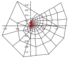
Figure 5: The discrete power function with $\gamma=0.25+3.35i$.

Remark 3.3

Agafonov has shown that the generalized discrete power function $f_{n,m}$, under the setting of $c_{0}=c_{1}=1$, $t=e^{2i\alpha}\,(0<\alpha<\pi)$ and $0<r<1$, is embedded [3].

Remark 3.4

As we mention above, some special solutions to (2.7) in terms of the $\tau$ functions of P_VI have been presented [12]. It is easy to show that these solutions also satisfy a difference equation which is a deformation of (2.3) in the sense that the coefficients $n$ and $m$ of (2.3) are replaced by arbitrary complex numbers. For instance, a class of solutions presented in Theorem 6 of [12] satisfies

$$\begin{array}[]{l}(\alpha_{0}+\alpha_{2}+\alpha_{4})f_{n,m}\\[2.84526pt] =(n-\alpha_{2})\dfrac{(f_{n+1,m}-f_{n,m})(f_{n,m}-f_{n-1,m})}{f_{n+1,m}-f_{n-1,m}}-(\alpha_{1}+\alpha_{2}+\alpha_{4}-m)\dfrac{(f_{n,m+1}-f_{n,m})(f_{n,m}-f_{n,m-1})}{f_{n,m+1}-f_{n,m-1}},\end{array}$$ (3.10)

where $\alpha_{i}$ are parameters of P_VI introduced in Appendix A. Setting the parameters as $(\alpha_{0},\alpha_{1},\alpha_{2},\alpha_{3},\alpha_{4})=(r,0,0,-r+1,0)$, we see that the above equation is reduced to (2.3) and that the solutions are given by the hypergeometric $\tau$ functions under the initial conditions (3.1).

3.2 Proof of the results

In this subsection, we give the proof of Theorem 3.1 and Proposition 3.2. One can easily verify that $f_{n,m}$ satisfies the initial condition (3.1) by noticing $\tau_{0}(a,b,c;t)=1$. We then show that $f_{n,m}$ and $v_{n,m}$ given in Theorem 3.1 and Proposition 3.2 satisfy the relation (2.8), the difference equation (2.3), the compatibility condition (2.9) and the similarity condition (2.11) by means of the various bilinear relations for the hypergeometric $\tau$ function. Note in advance that we use the bilinear relations by specializing the parameters $a,b$ and $c$ as

$$a=-N,\quad b=-r-N,\quad c=-r+1,\quad N=\frac{n+m}{2},$$ (3.11)

when $n+m$ is even, or

$$a=-r-N+1,\quad b=-N,\quad c=-r+1,\quad N=\frac{n+m+1}{2},$$ (3.12)

when $n+m$ is odd.

We first verify the relation (2.8). Note that we have the following bilinear relations

$$\begin{array}[]{l}(c-1)\tau_{n}^{0,-1,-1}\tau_{n+1}^{-1,-1,-1}=(c-b-1)t\tau_{n+1}^{0,-1,0}\tau_{n}^{-1,-1,-2}+b\tau_{n}^{0,0,0}\tau_{n+1}^{-1,-2,-2},\\[5.69054pt] (c-1)\tau_{n}^{-1,-1,-1}\tau_{n}^{0,-1,-1}=(c-b-1)\tau_{n}^{0,-1,0}\tau_{n}^{-1,-1,-2}+b\tau_{n}^{0,0,0}\tau_{n}^{-1,-2,-2},\end{array}$$ (3.13)

$$\begin{array}[]{l}(a-b)\tau_{m}^{0,-1,-1}\tau_{m}^{0,-1,0}=a\tau_{m}^{-1,-1,-1}\tau_{m}^{1,-1,0}-b\tau_{m}^{0,0,0}\tau_{m}^{0,-2,-1},\\[5.69054pt] (a-b)t\tau_{m+1}^{0,-1,0}\tau_{m}^{0,-1,-1}=a\tau_{m+1}^{-1,-1,-1}\tau_{m}^{1,-1,0}-b\tau_{m}^{0,0,0}\tau_{m+1}^{0,-2,-1},\end{array}$$ (3.14)

$$\begin{array}[]{l}(b-a+1)\tau_{m}^{0,0,0}\tau_{m}^{-1,-1,-1}=(b-c+1)\tau_{m}^{0,-1,0}\tau_{m}^{-1,0,-1}+(c-a)\tau_{m}^{0,-1,-1}\tau_{m}^{-1,0,0},\\[5.69054pt] (b-a+1)\tau_{m+1}^{-1,-1,-1}\tau_{m}^{0,0,0}=(b-c+1)\tau_{m+1}^{0,-1,0}\tau_{m}^{-1,0,-1}+(c-a)\tau_{m}^{0,-1,-1}\tau_{m+1}^{-1,0,0},\end{array}$$ (3.15)

for the hypergeometric $\tau$ functions, the derivation of which is discussed in Appendix A. Let us consider the case where $n^{\prime}=n$. When $n+m$ is even, the relation (2.8) is reduced to

$$\begin{array}[]{l}-r\tau_{n}^{[1,1,1]}\tau_{n+1}^{[0,1,1]}=Nt\tau_{n+1}^{[1,1,2]}\tau_{n}^{[0,1,0]}-(r+N)\tau_{n}^{[1,2,2]}\tau_{n+1}^{[0,0,0]},\\[2.84526pt] -r\tau_{n}^{[0,1,1]}\tau_{n}^{[1,1,1]}=N\tau_{n}^{[1,1,2]}\tau_{n}^{[0,1,0]}-(r+N)\tau_{n}^{[1,2,2]}\tau_{n}^{[0,0,0]},\end{array}$$ (3.16)

where we denote

$$\tau_{n^{\prime}}^{[i_{1},i_{2},i_{3}]}=\tau_{n^{\prime}}(-N+i_{1},-r-N+i_{2},-r+i_{3};t),$$ (3.17)

for simplicity. We see that the relations (3.16) can be obtained from (3.13) with the parameters specialized as (3.11). In fact, the hypergeometric $\tau$ functions can be rewritten as

$$\tau_{n}^{0,-1,-1}=\tau_{n}(a+1,b+1,c)=\tau_{n}(-N+1,-r-N+1,-r+1)=\tau_{n}^{[1,1,1]},$$ (3.18)

for instance. When $n+m$ is odd, (2.8) yields

$$\begin{array}[]{l}-r\tau_{n}^{[1,2,1]}\tau_{n+1}^{[1,1,1]}=(-r+N)t\tau_{n+1}^{[1,2,2]}\tau_{n}^{[1,1,0]}-N\tau_{n}^{[2,2,2]}\tau_{n+1}^{[0,1,0]},\\[2.84526pt] -r\tau_{n}^{[1,1,1]}\tau_{n}^{[1,2,1]}=(-r+N)\tau_{n}^{[1,2,2]}\tau_{n}^{[1,1,0]}-N\tau_{n}^{[2,2,2]}\tau_{n}^{[0,1,0]},\end{array}$$ (3.19)

which is also obtained from (3.13) by specializing the parameters as (3.12). Note that the hypergeometric $\tau$ functions can be rewritten as

$$\begin{array}[]{ll}\tau_{n}^{0,-1,-1}=\tau_{n}(a+1,b+1,c)\!\!\!&=\tau_{n}(-r-N+2,-N+1,-r+1)\\[2.84526pt] &=\tau_{n}(-N+1,-r-N+2,-r+1)=\tau_{n}^{[1,2,1]},\end{array}$$ (3.20)

this time. In the case where $n^{\prime}=m$, one can similarly verify the relation (2.8) by using the bilinear relations (3.14) and (3.15).

Next, we prove that (2.3) is satisfied, which is rewritten by using (2.8) as

$$-r\dfrac{f_{n,m}}{v_{n,m}}=\dfrac{nt^{-\frac{1}{2}}}{v_{n+1,m}^{-1}+v_{n-1,m}^{-1}}+\dfrac{m}{v_{n,m+1}^{-1}+v_{n,m-1}^{-1}}.$$ (3.21)

We use the bilinear relations

$$\begin{array}[]{l}n^{\prime}\tau_{n^{\prime}}^{0,0,0}\tau_{n^{\prime}}^{0,-1,-1}=(b-c+1)\tau_{n^{\prime}+1}^{0,-1,0}\tau_{n^{\prime}-1}^{0,0,-1}+at^{-1}\tau_{n^{\prime}+1}^{-1,-1,-1}\tau_{n^{\prime}-1}^{1,0,0},\\[5.69054pt] (a+b-c+n^{\prime}+1)\tau_{n^{\prime}}^{0,0,0}\tau_{n^{\prime}}^{0,-1,-1}=a\tau_{n^{\prime}}^{-1,-1,-1}\tau_{n^{\prime}}^{1,0,0}+(b-c+1)\tau_{n^{\prime}}^{0,-1,0}\tau_{n^{\prime}}^{0,0,-1},\end{array}$$ (3.22)

and

$$\begin{array}[]{l}\tau_{n}^{0,0,0}\tau_{n}^{-1,-1,-2}=-t^{-1}\tau_{n+1}^{-1,-1,-1}\tau_{n-1}^{0,0,-1}+\tau_{n}^{-1,-1,-1}\tau_{n}^{0,0,-1},\\[5.69054pt] \tau_{m}^{0,0,0}\tau_{m}^{1,-1,0}=\tau_{m}^{0,-1,0}\tau_{m}^{1,0,0}-\tau_{m+1}^{0,-1,0}\tau_{m-1}^{1,0,0},\\[5.69054pt] \tau_{m}^{0,-1,-1}\tau_{m}^{-1,0,-1}=-\tau_{m+1}^{-1,-1,-1}\tau_{m-1}^{0,0,-1}+\tau_{m}^{-1,-1,-1}\tau_{m}^{0,0,-1},\end{array}$$ (3.23)

for the proof. Their derivation is also shown in Appendix A. Let us consider the case where $n^{\prime}=n$. When $n+m$ is even, we have

$$\begin{array}[]{l}-n\tau_{n}^{[1,2,2]}\tau_{n}^{[1,1,1]}=N\tau_{n+1}^{[1,1,2]}\tau_{n-1}^{[1,2,1]}+Nt^{-1}\tau_{n+1}^{[0,1,1]}\tau_{n-1}^{[2,2,2]},\\[2.84526pt] m\tau_{n}^{[1,2,2]}\tau_{n}^{[1,1,1]}=N\tau_{n}^{[0,1,1]}\tau_{n}^{[2,2,2]}+N\tau_{n}^{[1,1,2]}\tau_{n}^{[1,2,1]},\end{array}$$ (3.24)

from the bilinear relations (3.22) by specializing the parameters $a,b$ and $c$ as given in (3.11). These lead us to

$$\begin{array}[]{l}v_{n+1,m}^{-1}+v_{n-1,m}^{-1}=c_{1}^{-1}t^{-r+\frac{n+1}{2}}\dfrac{n}{N}\dfrac{\tau_{n}^{[1,2,2]}\tau_{n}^{[1,1,1]}}{\tau_{n+1}^{[0,1,1]}\tau_{n-1}^{[1,2,1]}},\\[14.22636pt] v_{n,m+1}^{-1}+v_{n,m-1}^{-1}=-c_{1}^{-1}t^{-r+\frac{n}{2}}\dfrac{m}{N}\dfrac{\tau_{n}^{[1,2,2]}\tau_{n}^{[1,1,1]}}{\tau_{n}^{[0,1,1]}\tau_{n}^{[1,2,1]}}.\end{array}$$ (3.25)

By using

$$\tau_{n}^{[1,2,2]}\tau_{n}^{[0,1,0]}=-t^{-1}\tau_{n+1}^{[0,1,1]}\tau_{n-1}^{[1,2,1]}+\tau_{n}^{[0,1,1]}\tau_{n}^{[1,2,1]},$$ (3.26)

which is obtained from the first relation in (3.23), one can verify (3.21). When $n+m$ is odd, we have the bilinear relations

$$\begin{array}[]{l}-n\tau_{n}^{[2,2,2]}\tau_{n}^{[1,2,1]}=(-r+N)\tau_{n+1}^{[1,2,2]}\tau_{n-1}^{[2,2,1]}+(r+N-1)t^{-1}\tau_{n+1}^{[1,1,1]}\tau_{n-1}^{[2,3,2]},\\[2.84526pt] m\tau_{n}^{[2,2,2]}\tau_{n}^{[1,2,1]}=(r+N-1)\tau_{n}^{[1,1,1]}\tau_{n}^{[2,3,2]}+(-r+N)\tau_{n}^{[1,2,2]}\tau_{n}^{[2,2,1]},\end{array}$$ (3.27)

from (3.22) with (3.12), and

$$\tau_{n}^{[2,2,2]}\tau_{n}^{[1,1,0]}=-t^{-1}\tau_{n+1}^{[1,1,1]}\tau_{n-1}^{[2,2,1]}+\tau_{n}^{[1,1,1]}\tau_{n}^{[2,2,1]},$$ (3.28)

from the first relation in (3.23). These lead us to (3.21). We next consider the case where $n^{\prime}=m$. When $n+m$ is even, we get the bilinear relations

$$\begin{array}[]{l}-m\tau_{m}^{[1,2,2]}\tau_{m}^{[1,1,1]}=N\tau_{m+1}^{[1,1,2]}\tau_{m-1}^{[1,2,1]}+Nt^{-1}\tau_{m+1}^{[0,1,1]}\tau_{m-1}^{[2,2,2]},\\[2.84526pt] n\tau_{m}^{[1,2,2]}\tau_{m}^{[1,1,1]}=N\tau_{m}^{[0,1,1]}\tau_{m}^{[2,2,2]}+N\tau_{m}^{[1,1,2]}\tau_{m}^{[1,2,1]},\end{array}$$ (3.29)

and

$$\tau_{m}^{[1,2,2]}\tau_{m}^{[2,1,2]}=\tau_{m}^{[1,1,2]}\tau_{m}^{[2,2,2]}-\tau_{m+1}^{[1,1,2]}\tau_{m-1}^{[2,2,2]},$$ (3.30)

from (3.22) and the second relation in (3.23), respectively. By using these relations, one can show (3.21) in a similar way to the case where $n^{\prime}=n$. When $n+m$ is odd, we use the bilinear relations

$$\begin{array}[]{l}-m\tau_{m}^{[2,2,2]}\tau_{m}^{[1,2,1]}=(-r+N)\tau_{m+1}^{[1,2,2]}\tau_{m-1}^{[2,2,1]}+(r+N-1)t^{-1}\tau_{m+1}^{[1,1,1]}\tau_{m-1}^{[2,3,2]},\\[2.84526pt] n\tau_{m}^{[2,2,2]}\tau_{m}^{[1,2,1]}=(r+N-1)\tau_{m}^{[1,1,1]}\tau_{m}^{[2,3,2]}+(-r+N)\tau_{m}^{[1,2,2]}\tau_{m}^{[2,2,1]},\end{array}$$ (3.31)

and

$$\tau_{m}^{[1,2,1]}\tau_{m}^{[2,1,1]}=-\tau_{m+1}^{[1,1,1]}\tau_{m-1}^{[2,2,1]}+\tau_{m}^{[1,1,1]}\tau_{m}^{[2,2,1]},$$ (3.32)

which are obtained from (3.22) and the third relation in (3.23), respectively, to show (3.21).

We next give the verification of the compatibility condition (2.9) by using the bilinear relations

$$\begin{array}[]{l}(c-a)\tau_{n^{\prime}}^{0,-1,-1}\tau_{n^{\prime}+1}^{-1,-1,0}-b\tau_{n^{\prime}}^{0,0,0}\tau_{n^{\prime}+1}^{-1,-2,-1}=(t-1)\tau_{n^{\prime}}^{-1,-1,-1}\tau_{n^{\prime}+1}^{0,-1,0},\\[5.69054pt] (c-a)t\tau_{n^{\prime}}^{0,-1,-1}\tau_{n^{\prime}+1}^{-1,-1,0}-b\tau_{n^{\prime}}^{0,0,0}\tau_{n^{\prime}+1}^{-1,-2,-1}=(t-1)\tau_{n^{\prime}}^{0,-1,0}\tau_{n^{\prime}+1}^{-1,-1,-1}.\end{array}$$ (3.33)

The derivation of these is discussed in Appendix A. We first consider the case where $n^{\prime}=n$. When $n+m$ is even, we get

$$\begin{array}[]{l}(-r+N+1)\tau_{n}^{[1,1,1]}\tau_{n+1}^{[0,1,2]}+(r+N)\tau_{n}^{[1,2,2]}\tau_{n+1}^{[0,0,1]}=(t-1)\tau_{n}^{[0,1,1]}\tau_{n+1}^{[1,1,2]},\\[2.84526pt] (-r+N+1)t\tau_{n}^{[1,1,1]}\tau_{n+1}^{[0,1,2]}+(r+N)\tau_{n}^{[1,2,2]}\tau_{n+1}^{[0,0,1]}=(t-1)\tau_{n}^{[1,1,2]}\tau_{n+1}^{[0,1,1]},\end{array}$$ (3.34)

from the bilinear relations (3.33). Then we have

$$\begin{array}[]{l}t^{\frac{1}{2}}v_{n,m}+v_{n+1,m+1}=t^{-\frac{n+1}{2}}(t-1)\dfrac{(r)_{N}}{(-r+1)_{N+1}}\dfrac{\tau_{n}^{[1,1,2]}\tau_{n+1}^{[0,1,1]}}{\tau_{n}^{[1,2,2]}\tau_{n+1}^{[0,1,2]}},\\[14.22636pt] v_{n,m}+t^{\frac{1}{2}}v_{n+1,m+1}=t^{-\frac{n}{2}}(t-1)\dfrac{(r)_{N}}{(-r+1)_{N+1}}\dfrac{\tau_{n}^{[0,1,1]}\tau_{n+1}^{[1,1,2]}}{\tau_{n}^{[1,2,2]}\tau_{n+1}^{[0,1,2]}},\end{array}$$ (3.35)

from which we arrive at the compatibility condition (2.9). When $n+m$ is odd, we have

$$\begin{array}[]{l}N\tau_{n}^{[1,2,1]}\tau_{n+1}^{[1,1,2]}+N\tau_{n}^{[2,2,2]}\tau_{n+1}^{[0,1,1]}=(t-1)\tau_{n}^{[1,1,1]}\tau_{n+1}^{[1,2,2]},\\[2.84526pt] Nt\tau_{n}^{[1,2,1]}\tau_{n+1}^{[1,1,2]}+N\tau_{n}^{[2,2,2]}\tau_{n+1}^{[0,1,1]}=(t-1)\tau_{n}^{[1,2,2]}\tau_{n+1}^{[1,1,1]},\end{array}$$ (3.36)

from (3.33). Calculating $t^{\frac{1}{2}}v_{n,m}+v_{n+1,m+1}$ and $v_{n,m}+t^{\frac{1}{2}}v_{n+1,m+1}$ by means of these relations, we see that we have (2.9). In the case where $n^{\prime}=m$, one can verify the compatibility condition (2.9) in a similar manner.

Let us finally verify the similarity condition (2.11), which can be written as

$$\dfrac{n}{2}-\dfrac{1}{2}\chi_{n+m}-t\dfrac{d}{dt}\log v_{n,m}=\dfrac{nv_{n+1,m}}{v_{n+1,m}+v_{n-1,m}}.$$ (3.37)

Here, we take the factor $\chi_{n+m}$ as $\chi_{n+m}=r\left[(-1)^{n+m}-1\right]$. The relevant bilinear relations for the hypergeometric $\tau$ function are

$$\begin{array}[]{l}(D+n)\tau_{n}^{0,0,0}\cdot\tau_{n}^{0,-1,-1}=at^{-1}\tau_{n+1}^{-1,-1,-1}\tau_{n-1}^{1,0,0},\\[2.84526pt] (D+b-c+1)\tau_{m}^{0,-1,-1}\cdot\tau_{m}^{0,0,0}=(b-c+1)\tau_{m}^{0,-1,0}\tau_{m}^{0,0,-1},\\[2.84526pt] (D+a+m)\tau_{m}^{0,0,0}\cdot\tau_{m}^{0,-1,-1}=a\tau_{m}^{-1,-1,-1}\tau_{m}^{1,0,0}.\end{array}$$ (3.38)

The derivation of these is obtained in Appendix A. We first consider the case where $n^{\prime}=n$. When $n+m$ is even, it is easy to see that we have

$$n\dfrac{v_{n+1,m}}{v_{n+1,m}+v_{n-1,m}}=-Nt^{-1}\dfrac{\tau_{n+1}^{[0,1,1]}\tau_{n-1}^{[2,2,2]}}{\tau_{n}^{[1,2,2]}\tau_{n}^{[1,1,1]}},$$ (3.39)

from the bilinear relation (3.24). We get

$$(D+n)\tau_{n}^{[1,2,2]}\cdot\tau_{n}^{[1,1,1]}=-Nt^{-1}\tau_{n+1}^{[0,1,1]}\tau_{n-1}^{[2,2,2]},$$ (3.40)

from the first relation in (3.38) with (3.11). From this we can obtain the similarity condition (3.37) as follows. When $n+m$ is odd, we have

$$(D+n)\tau_{n}^{[2,2,2]}\cdot\tau_{n}^{[1,2,1]}=-t^{-1}(r+N-1)\tau_{n+1}^{[1,1,1]}\tau_{n-1}^{[2,3,2]},$$ (3.41)

from the first relation in (3.38). This relation together with the first relation in (3.27) leads us to (3.37). Next, we discuss the case where $n^{\prime}=m$. When $n+m$ is even, we have

$$(D+N)\tau_{m}^{[1,2,2]}\cdot\tau_{m}^{[1,1,1]}=N\tau_{m}^{[1,1,2]}\tau_{m}^{[1,2,1]},$$ (3.42)

from the second relation in (3.38). Then we arrive at (3.37) by virtue of the second relation in (3.29). When $n+m$ is odd, we get

$$\textstyle(D+r+\frac{n-m-1}{2})\tau_{m}^{[1,2,1]}\cdot\tau_{m}^{[2,2,2]}=(r+N-1)\tau_{m}^{[1,1,1]}\tau_{m}^{[2,3,2]},$$ (3.43)

from the third relation in (3.38). Then we derive the similarity condition (3.37) by using the second relation in (3.31). This completes the proof of Theorem 3.1 and Proposition 3.2.

4 Extension of the domain

First, we extend the domain of the discrete power function to $\mathbb{Z}^{2}$. To determine the values of $f_{n,m}$ in the second, third and fourth quadrants, we have to give the values of $f_{-1,0}$ and $f_{0,-1}$ as the initial conditions. Set the initial conditions as

$$f_{-1,0}=c_{2}t^{2r},\quad f_{0,-1}=c_{3}t^{3r},$$ (4.1)

where $c_{2}$ and $c_{3}$ are arbitrary constants. This is natural because these conditions reduce to

$$f_{1,0}=1,\quad f_{0,1}=e^{\pi ir},\quad f_{-1,0}=e^{2\pi ir},\quad f_{0,-1}=e^{3\pi ir}$$ (4.2)

at the original setting. Due to the symmetry of equations (2.7) and (2.3), we immediately obtain the explicit formula of $f_{n,m}$ in the second and third quadrant.

Corollary 4.1

Under the initial conditions $f_{0,1}=c_{1}t^{r}$ and (4.1), we have

$$\begin{array}[]{l}f_{-n,m}=f_{n,m}|_{\,c_{0}\mapsto c_{2}t^{2r}},\quad f_{-n,-m}=f_{n,m}|_{\,c_{0}\mapsto c_{2}t^{2r},c_{1}\mapsto c_{3}t^{2r}},\end{array}$$ (4.3)

for $n,m\in\mathbb{Z}_{+}$.

Next, let us discuss the explicit formula in the fourth quadrant. Naively, we use the initial conditions $f_{0,-1}=c_{3}t^{3r}$ and $f_{1,0}=c_{0}$ to get the formula $f_{n,-m}=f_{n,m}|_{\,c_{1}\mapsto c_{3}t^{2r}}$. However, this setting makes the discrete power function $f_{n,m}$ become a single-valued function on $\mathbb{Z}^{2}$. In order to allow $f_{n,m}$ to be multi-valued on $\mathbb{Z}^{2}$, we introduce a discrete analogue of the Riemann surface by the following procedure. Prepare an infinite number of $\mathbb{Z}^{2}$-planes, cut the positive part of the “real axis” of each $\mathbb{Z}^{2}$-plane and glue them in a similar way to the continuous case. The next step is to write the initial conditions (3.1) and (4.1) in polar form as

$$f(1,\pi k/2)=c_{k}t^{kr}\quad(k=0,1,2,3),$$ (4.4)

where the first component, $1$, denotes the absolute value of $n+im$ and the second component, $\pi k/2$, is the argument. We must generalize the above initial conditions to those for arbitrary $k\in\mathbb{Z}$ so that we obtain the explicit expression of $f_{n,m}$ for each quadrant of each $\mathbb{Z}^{2}$-plane. Let us illustrate a typical case. When $\dfrac{3}{2}\pi\leq\arg(n+im)\leq 2\pi$, we solve the equations (2.7) and (2.3) under the initial conditions

$$f(1,3\pi/2)=c_{3}t^{3r},\quad f(1,2\pi)=c_{4}t^{4r},$$ (4.5)

to obtain the formula

$$f_{-n,-m}=f_{n,m}|_{\,c_{0}\mapsto c_{4}t^{4r},c_{1}\mapsto c_{3}t^{2r}}\quad(n,m\in\mathbb{Z}_{+}).$$ (4.6)

We present the discrete power function with $\gamma=5/2$ whose domain is $\mathbb{Z}^{2}$ and the discrete Riemann surface in Figure 7 and 7, respectively. Note that the necessary and sufficient condition for the discrete power function to reduce to a single-valued function on $\mathbb{Z}^{2}$ is ($c_{k}=c_{k+4}$ and) $e^{4\pi ir}=1$, which means that the exponent $\gamma$ is an integer.

Figure 6: The discrete power function with $\gamma=5/2$ whose domain is $\mathbb{Z}^{2}$.

Figure 7: The discrete power function with $\gamma=5/2$ whose domain is the discrete Riemann surface.

5 Associated circle pattern of Schramm type

Agafonov and Bobenko have shown that the discrete power function for real $\gamma$ is an immersion and thus defines a circle pattern of Schramm type. We have generalized the discrete power function to complex $\gamma$. It is natural to ask whether there are other cases where the discrete power function is associated with circle patterns. We have the following result:

Theorem 5.1

The mapping $f:\,\mathbb{Z}^{2}_{+}\to\mathbb{C}\,;(n,m)\mapsto f_{n,m}$ satisfying (2.1) and (2.3) with the initial condition

$$f_{0,0}=0,\quad f_{1,0}=1,\quad f_{0,1}=e^{\pi i\gamma/2},\quad\gamma\in\mathbb{C}$$ (5.1)

is an immersion when ${\rm Re}~{}\gamma=1$.

In this section, we give the proof of Theorem 5.1 along with the discussion in [4]. We also use the explicit formulae given in previous sections.

5.1 Circle pattern

Setting

$$\gamma=1+i\delta,\quad\delta\in\mathbb{R},$$ (5.2)

we associate the discrete power function with circle patterns of Schramm type. The proof of Theorem 5.1 is then reduced to properties of the radii of those circles.

Lemma 5.1

A discrete power function $f_{n,m}$ defined by (2.1) and (2.3) with initial condition

$$f_{0,0}=0,\quad f_{1,0}=1,\quad f_{0,1}=c_{1}e^{\pi i\gamma/2},\quad c_{1}>0$$ (5.3)

for arbitrary $\gamma\in\mathbb{C}\backslash{2\mathbb{Z}}$ has the equidistant property

$$f_{2n,0}-f_{2n-1,0}=f_{2n+1,0}-f_{2n,0},\quad f_{0,2m}-f_{0,2m-1}=f_{0,2m+1}-f_{0,2m},$$ (5.4)

for any $n\geq 1,m\geq 1$. Moreover, if and only if ${\rm Re}~{}\gamma=1$, we have

$$|f_{n+1,0}-f_{n,0}|=|f_{n,0}-f_{n-1,0}|,\quad|f_{0,m+1}-f_{0,m}|=|f_{0,m}-f_{0,m-1}|,$$ (5.5)

for any $n\geq 1,m\geq 1$.

Proof. By using the formulae in Theorem 3.1 (or Proposition 3.2), we have

$$\begin{split}&f_{2n,0}-f_{2n-1,0}=f_{2n+1,0}-f_{2n,0}=\frac{\gamma}{2n+\gamma}\prod_{k=1}^{n}\frac{2k+\gamma}{2k-\gamma},\\ &f_{0,2m}-f_{0,2m-1}=f_{0,2m+1}-f_{0,2m}=c_{1}e^{\frac{\pi i\gamma}{2}}\frac{\gamma}{2m+\gamma}\prod_{k=1}^{m}\frac{2k+\gamma}{2k-\gamma},\end{split}$$ (5.6)

which proves (5.4). We also have

$$f_{2n+2,0}-f_{2n+1,0}=\prod_{k=1}^{n+1}\frac{2k-2+\gamma}{2k-\gamma},\quad f_{2n+1,0}-f_{2n,0}=\prod_{k=1}^{n}\frac{2k-2+\gamma}{2k-\gamma}.$$ (5.7)

Putting $\gamma=1+i\delta$, we obtain

$$f_{2n+2,0}-f_{2n+1,0}=\prod_{k=1}^{n+1}\frac{2k-1+i\delta}{2k-1-i\delta},\quad f_{2n+1,0}-f_{2n,0}=\prod_{k=1}^{n}\frac{2k-1+i\delta}{2k-1-i\delta},$$ (5.8)

which implies $|f_{2n+2,0}-f_{2n+1,0}|=|f_{2n+1,0}-f_{2n,0}|=1$. Using the first equation of (5.4), we see that the first equation of (5.5) follows. The second equation of (5.5) can be proved in a similar manner. Suppose that (5.5) holds, then from (5.7) we have

$$\left|\frac{f_{2n+2,0}-f_{2n+1,0}}{f_{2n+1,0}-f_{2n,0}}\right|=\left|\frac{2n+\gamma}{2n+2-\gamma}\right|=1,$$ (5.9)

which leads us to ${\rm Re}~{}\gamma=1$.  $\square$

Proposition 5.2

Let $f_{n,m}$ satisfy (2.1) and (2.3) in $\mathbb{Z}^{2}_{+}$ with initial condition (5.3). Then all the elementary quadrilaterals $(f_{n,m},f_{n+1,m},f_{n+1,m+1},f_{n,m+1})$ are of the kite form, namely, all edges at each vertex $f_{n,m}$ with $n+m=1\,(\mbox{mod}\,2)$ are of the same length,

$$|f_{n+1,m}-f_{n,m}|=|f_{n,m+1}-f_{n,m}|=|f_{n-1,m}-f_{n,m}|=|f_{n,m-1}-f_{n,m}|.$$ (5.10)

Moreover, all angles between the neighbouring edges at the vertex $f_{n,m}$ with $n+m=0\,(\mbox{mod}\,2)$ are equal to $\pi/2$.

Proof. For three complex numbers $z_{i}$ ($i=1,2,3$), we introduce a notation

$$[z_{1},z_{2},z_{3}]=\arg\frac{z_{1}-z_{2}}{z_{3}-z_{2}}.$$ (5.11)

We first consider the quadrilateral $(f_{0,0},f_{1,0},f_{1,1},f_{0,1})$. Notice that $f_{0,1}=ic_{1}e^{-\frac{\pi\delta}{2}}$ which implies that $[f_{0,1},f_{0,0},f_{1,0}]=\frac{\pi}{2}$. Then it follows from (2.1) that $[f_{1,0},f_{1,1},f_{0,1}]=\frac{\pi}{2}$, $|f_{1,0}-f_{0,0}|=|f_{1,1}-f_{1,0}|$ and $|f_{0,1}-f_{0,0}|=|f_{1,1}-f_{0,1}|$. We next consider the quadrilateral $(f_{1,0},f_{2,0},f_{2,1},f_{1,1})$ where, from Lemma 5.1, we have $|f_{1,1}-f_{1,0}|=|f_{2,0}-f_{1,0}|$. We see from (2.1) that $[f_{2,1},f_{1,1},f_{1,0}]=[f_{1,0},f_{2,0},f_{2,1}]=\frac{\pi}{2}$ and $|f_{2,1}-f_{1,1}|=|f_{2,1}-f_{2,0}|$. From Lemma 5.1 and $[f_{1,0},f_{2,0},f_{2,1}]=\frac{\pi}{2}$, we see that $[f_{2,1},f_{2,0},f_{3,0}]=\frac{\pi}{2}$. Then a similar argument can be applied to the quadrilateral $(f_{2,0},f_{3,0},f_{3,1},f_{2,1})$ and so forth. In this manner, Proposition 5.2 is proved inductively.  $\square$

From Proposition 5.2, it follows that the circumscribed circles of the quadrilaterals $(f_{n-1,m},f_{n,m-1},f_{n+1,m},f_{n,m+1})$ with $n+m=1\,(\mbox{mod}\,2)$ form a circle pattern of Schramm type [4, 16], namely, the circles of neighbouring quadrilaterals intersect orthogonally and the circles of half-neighbouring quadrilaterals with a common vertex are tangent (See Figure 8).

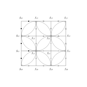
Figure 8: A schematic diagram of quadrilaterals.

Conversely, for a given circle pattern of Schramm type, it is possible to construct a discrete conformal mapping $f_{n,m}$ as follows. Let $\{C_{n,m}\},\,(n,m)\in{\bf V}=\{(n,m)\in\mathbb{Z}_{+}^{2}\,|\,n+m=1\,(\mbox{mod}\,2)\}$ be a circle pattern of Schramm type on the complex plane. Define $f\,:\,\mathbb{Z}_{+}^{2}\to\mathbb{C}\,;\,(n,m)\mapsto f_{n,m}$ in the following manner:

• If $n+m=1\,(\mbox{mod}\,2)$, then $f_{n,m}$ is the center of $C_{n,m}$.

• If $n+m=0\,(\mbox{mod}\,2)$, then $f_{n,m}:=C_{n-1,m}\cap C_{n+1,m}=C_{n,m+1}\cap C_{n,m-1}$.

By construction, it follows that all elementary quadrilaterals $(f_{n,m},f_{n+1,m},f_{n+1,m+1},f_{n,m+1})$ are of the kite form whose angles between the edges with different lengths are $\frac{\pi}{2}$. Therefore, (2.1) is satisfied automatically. In what follows, the function $f_{n,m}$, defined by (a) and (b), is called a discrete conformal map corresponding to the circle pattern $\{C_{n,m}\}$.

We now use the the radii of corresponding circle patterns to characterize the necessary and sufficient condition that the discrete power function is an immersion.

Theorem 5.3

Let $f_{n,m}$ satisfying (2.1) and (2.3) with initial condition (5.3) be an immersion. Then $R_{n,m}$ defined by

$$R_{n,m}=|f_{n+1,m}-f_{n,m}|=|f_{n,m+1}-f_{n,m}|=|f_{n-1,m}-f_{n,m}|=|f_{n,m-1}-f_{n,m}|$$ (5.12)

satisfies

$$n\dfrac{R_{n+1,m}-R_{n-1,m}}{R_{n+1,m}+R_{n-1,m}}+m\dfrac{R_{n,m+1}-R_{n,m-1}}{R_{n,m+1}+R_{n,m-1}}=0,$$ (5.13)

and

$$R_{n+1,m+2}=\dfrac{[(m+1)R_{n,m+1}+\delta R_{n+1,m}]R_{n,m+1}(R_{n+1,m}+R_{n-1,m})+nR_{n+1,m}(R_{n,m+1}^{2}-R_{n+1,m}R_{n-1,m})}{[(m+1)R_{n+1,m}-\delta R_{n,m+1}](R_{n+1,m}+R_{n-1,m})-n(R_{n,m+1}^{2}-R_{n+1,m}R_{n-1,m})},$$ (5.14)

for $(n,m)\in{\bf V}$. Conversely, let $R\,:\,{\bf V}\to\mathbb{R}_{+}$ satisfy (5.13) and (5.14). Then $R_{n,m}$ defines an immersed circle pattern of Schramm type. The corresponding discrete conformal map $f_{n,m}$ is an immersion and satisfies (2.3).

Proof. The proof of Theorem 5.3 occupies the remainder of this subsection. Suppose that the discrete power function $f_{n,m}$ is immersed. For $n+m=0\,(\mbox{mod}\,2)$, we may parametrize the edges around the vertex $f_{n,m}$ as

$$f_{n+1,m}-f_{n,m}=r_{1}e^{i\beta},\quad f_{n,m+1}-f_{n,m}=ir_{2}e^{i\beta},\quad f_{n-1,m}-f_{n,m}=-r_{3}e^{i\beta},\quad f_{n,m-1}-f_{n,m}=-ir_{4}e^{i\beta},$$ (5.15)

where $r_{i}>0$ ($i=1,2,3,4$) are the radii of the corresponding circles, since all the angles around $f_{n,m}$ are $\frac{\pi}{2}$. The constraint (2.3) reads

$$\gamma f_{n,m}=e^{i\beta}\left(2n\dfrac{r_{1}r_{3}}{r_{1}+r_{3}}+2im\dfrac{r_{2}r_{4}}{r_{2}+r_{4}}\right).$$ (5.16)

Lemma 5.4

For $n+m=0\,(\mbox{mod}\,2)$ we have:

$$f_{n+1,m+1}-f_{n+1,m}=-e^{i\beta}r_{1}\dfrac{r_{1}-ir_{2}}{r_{1}+ir_{2}},\quad f_{n+1,m}-f_{n+1,m-1}=e^{i\beta}r_{1}\dfrac{r_{1}+ir_{4}}{r_{1}-ir_{4}}.$$ (5.17)

Proof. The kite form of the quadrilateral $(f_{n,m},f_{n+1,m},f_{n+1,m+1},f_{n,m+1})$ implies $f_{n+1,m+1}-f_{n+1,m}=-(f_{n+1,m}-f_{n,m})e^{-2i[f_{n,m+1},f_{n+1,m},f_{n+1,m+1}]}$ (See Figure 9). The first equation of (5.17) follows by noticing that $\tan[f_{n,m+1},f_{n+1,m},f_{n+1,m+1}]=\frac{r_{2}}{r_{1}}$. The second equation is derived by a similar consideration on the quadrilateral $(f_{n,m-1},f_{n+1,m-1},f_{n+1,m},f_{n,m})$.  $\square$

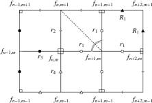
Figure 9: Parametrization of edges.

Setting $f_{n+2,m}-f_{n+1,m}=r_{1}e^{i(\beta+\sigma)}$ and substituting (5.15)–(5.17) into (2.3) at the point $(n+1,m)$, one arrives at

$$2n\dfrac{r_{1}r_{3}}{r_{1}+r_{3}}+2im\dfrac{r_{2}r_{4}}{r_{2}+r_{4}}+\gamma r_{1}=2(n+1)r_{1}\dfrac{1}{1+e^{-i\sigma}}+2mr_{1}\dfrac{r_{1}(r_{2}-r_{4})+i(r_{1}^{2}+r_{2}r_{4})}{2r_{1}(r_{2}+r_{4})}.$$ (5.18)

The real part of (5.18) gives

$$n\dfrac{r_{1}-r_{3}}{r_{1}+r_{3}}+m\dfrac{r_{2}-r_{4}}{r_{2}+r_{4}}=0,$$ (5.19)

which coincides with (5.13).

Now we parametrize the edges around the vertex $f_{n+1,m+1}$ with $n+m=0~{}({\rm mod}~{}2)$ as

$$\begin{split}&f_{n+2,m+1}=f_{n+1,m+1}+R_{1}e^{i\beta^{\prime}},\quad f_{n+1,m+2}=f_{n+1,m+1}+iR_{2}e^{i\beta^{\prime}},\\[5.69054pt] &f_{n,m+1}=f_{n+1,m+1}-r_{2}e^{i\beta^{\prime}},\quad f_{n+1,m}=f_{n+1,m+1}-ir_{1}e^{i\beta^{\prime}}.\end{split}$$ (5.20)

From the first equation of (5.17) and noticing that all angles around the vertex $f_{n+1,m+1}$ are $\frac{\pi}{2}$, we have the following relation between $\beta^{\prime}$ and $\beta$:

$$e^{i\beta^{\prime}}=ie^{i\beta}\dfrac{r_{1}-ir_{2}}{r_{1}+ir_{2}}.$$ (5.21)

One can express $f_{n+2,m+1}$ in two ways as (See Figure 9)

$$f_{n+2,m+1}=f_{n+2,m}+iR_{1}e^{i(\beta+\sigma)}=f_{n+1,m}+r_{1}e^{i(\beta+\sigma)}+iR_{1}e^{i(\beta+\sigma)},$$ (5.22)

and

$$f_{n+2,m+1}=f_{n+1,m+1}+R_{1}e^{i\beta^{\prime}}=f_{n+1,m}-e^{i\beta}r_{1}\dfrac{r_{1}-ir_{2}}{r_{1}+ir_{2}}+R_{1}e^{i\beta^{\prime}}.$$ (5.23)

The compatibility implies

$$e^{i\sigma}=\dfrac{R_{1}+ir_{1}}{R_{1}-ir_{1}}\dfrac{r_{1}-ir_{2}}{r_{1}+ir_{2}}.$$ (5.24)

Then, from the imaginary part of (5.18), one obtains

$$m\dfrac{r_{2}r_{4}-r_{1}^{2}}{r_{2}+r_{4}}+\delta r_{1}=(n+1)\dfrac{r_{1}^{2}-r_{2}R_{1}}{r_{2}+R_{1}},$$ (5.25)

or solving (5.25) with respect to $R_{1}=R_{n+2,m+1}$

$$R_{n+2,m+1}=\dfrac{[(n+1)R_{n+1,m}-\delta R_{n,m+1}]R_{n+1,m}(R_{n,m+1}+R_{n,m-1})+mR_{n,m+1}(R_{n+1,m}^{2}-R_{n,m+1}R_{n,m-1})}{[(n+1)R_{n,m+1}+\delta R_{n+1,m}](R_{n,m+1}+R_{n,m-1})-m(R_{n+1,m}^{2}-R_{n,m+1}R_{n,m-1})}.$$ (5.26)

We may rewrite (2.3) at $(n+1,m+1)$ in terms of $r_{i}$ ($i=1,2,3,4$) $R_{1}$, $R_{2}$ as

$$\begin{split}&2n\dfrac{r_{1}r_{3}}{r_{1}+r_{3}}+2im\dfrac{r_{2}r_{4}}{r_{2}+r_{4}}+\gamma r_{1}\left(1-\dfrac{r_{1}-ir_{2}}{r_{1}+ir_{2}}\right)\\[11.38109pt] &=i\dfrac{r_{1}-ir_{2}}{r_{1}+ir_{2}}\left[2(n+1)\dfrac{r_{2}R_{1}}{r_{2}+R_{1}}+2i(m+1)\dfrac{r_{1}R_{2}}{r_{1}+R_{2}}\right].\end{split}$$ (5.27)

Eliminating $\gamma$ from (5.18) and (5.27), we get

$$m\dfrac{r_{2}}{r_{2}+r_{4}}-n\dfrac{r_{3}}{r_{1}+r_{3}}-(m+1)\dfrac{R_{2}}{r_{1}+R_{2}}+(n+1)\dfrac{r_{2}}{r_{2}+R_{1}}=0.$$ (5.28)

We then eliminate $R_{1}$ using (5.25) to obtain

$$R_{2}=\dfrac{[(m+1)r_{2}+\delta r_{1}]r_{2}(r_{1}+r_{3})+nr_{1}(r_{2}^{2}-r_{1}r_{3})}{[(m+1)r_{1}-\delta r_{2}](r_{1}+r_{3})-n(r_{2}^{2}-r_{1}r_{3})},$$ (5.29)

which coincides with (5.14). This proves the first part of Theorem 5.3.

To prove the second part, we use the following lemma.

Lemma 5.5

Let $R\,:\,\bf{V}\to\mathbb{R}_{+}$ satisfy (5.13) and (5.14). Then, $R$ satisfies (5.26) and

$$\begin{array}[]{l}\left[(n+1)(R_{n+1,m}^{2}-R_{n,m-1}R_{n+2,m-1})+\delta R_{n+1,m}(R_{n,m-1}+R_{n+2,m-1})\right](R_{n,m+1}+R_{n,m-1})\\[5.69054pt] -m(R_{n+1,m}^{2}-R_{n,m+1}R_{n,m-1})(R_{n,m-1}+R_{n+2,m-1})=0.\end{array}$$ (5.30)

Proof. Substituting (5.13) at $(n,m)$ and at $(n+1,m+1)$ into (5.14) to eliminate $R_{n-1,m}$ and $R_{n+1,m+2}$, we get (5.26). Substituting (5.14) at $(n+1,m-1)$ into (5.26), we get (5.30) under the condition $\delta R_{n+1,m}(R_{n+2,m-1}-R_{n,m+1})+(n+m+1)(R_{n+2,m-1}R_{n,m+1}+R_{n+1,m}^{2})\neq 0$ which can be verified from the compatibility with (5.13) and (5.14).   $\square$

Eliminating $\delta$ from (5.26) and (5.30), we get

$$(R_{n+1,m}^{2}-R_{n,m+1}R_{n+2,m+1})(R_{n,m-1}+R_{n+2,m-1})+(R_{n+1,m}^{2}-R_{n,m-1}R_{n+2,m-1})(R_{n,m+1}+R_{n+2,m+1})=0.$$ (5.31)

In [16], it was proven that, given $R_{n,m}$ satisfying (5.31), the circle pattern with radii of the circles $R_{n,m}$ is immersed. Thus, the corresponding discrete conformal map $f_{n,m}$ is an immersion.

Let us finally show that the discrete conformal map $f_{n,m}$ satisfies (2.3). Putting $m=0$ in (5.13), we have $R_{n+1,0}=R_{n-1,0}$. This means that $|f_{n+1,0}-f_{n,0}|=|f_{n,0}-f_{n-1,0}|$ for any $n\geq 1$. By using the ambiguity of translation and scaling of the circle pattern, one can set $f_{0,0}=0,\,f_{1,0}=1$ without loss of generality, and set

$$f_{2N+1,0}-f_{2N,0}=f_{2N,0}-f_{2N-1,0}=\exp\left(2i\sum_{j=1}^{N}\theta_{j}\right)\quad(N=1,2,\ldots).$$ (5.32)

Putting $(n,m)=(2N,0)$ in (5.26) we have

$$\delta=(2N+1)\dfrac{R_{2N+1,0}^{2}-R_{2N,1}R_{2N+2,1}}{R_{2N+1,0}(R_{2N,1}+R_{2N+2,1})}.$$ (5.33)

A geometric consideration leads us the following lemma:

Lemma 5.6

We have

$$\delta=(2N+1)\tan\theta_{N+1}\quad(N=0,1,\ldots).$$ (5.34)

Proof.

(i) $0\leq 2\theta\leq\frac{\pi}{2}$

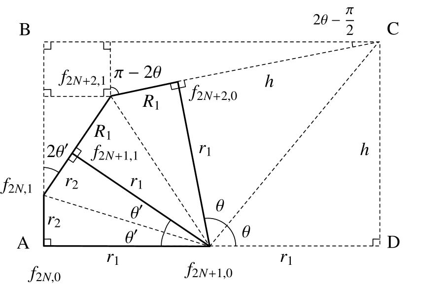
(ii) $\frac{\pi}{2}\leq 2\theta<\pi$

Figure 10: Configuration of points in Lemma 5.6.

First, we consider the case of $0\leq 2\theta\leq\pi/2$, see Figure 10 (i). From ${\rm BC}={\rm AD}$ we obtain

$$(r_{2}+R_{1})\sin 2\theta^{\prime}+(h+R_{1})\sin 2\theta=2r_{1},$$ (5.35)

which yields

$$(r_{2}h+r_{1}^{2})\left[(r_{2}+R_{1})h+(r_{2}R_{1}-r_{1}^{2})\right]=0.$$ (5.36)

Since $r_{2}h+r_{1}^{2}>0$, we have $h=\dfrac{r_{1}^{2}-r_{2}R_{1}}{r_{2}+R_{1}}$ and

$$\tan\theta=\dfrac{r_{1}^{2}-r_{2}R_{1}}{r_{1}(r_{2}+R_{1})}.$$ (5.37)

Thus we get (5.34) from (5.33). When $\pi/2\leq 2\theta<\pi$, the configuration of points is shown in Figure 10 (ii). The equality ${\rm BC}={\rm AD}$ implies

$$(r_{2}+R_{1})\sin 2\theta^{\prime}+(h+R_{1})\sin(\pi-2\theta)=2r_{1},$$ (5.38)

which gives the same result as the case of $0\leq 2\theta\leq\pi/2$. Let us investigate the case of $-\pi/2\leq 2\theta\leq 0$, see Figure 11 (i). Since ${\rm DC}={\rm AB}$ we have

$$(h+R_{1})\cos 2\theta+(r_{2}+R_{1})\cos(\pi-2\theta^{\prime})=h+r_{2},$$ (5.39)

which leads us to

$$(r_{2}h+r_{1}^{2})\left[(r_{2}R_{1}-r_{1}^{2})h-r_{1}^{2}(r_{2}+R_{1})\right]=0.$$ (5.40)

(i) $-\frac{\pi}{2}\leq 2\theta\leq 0$

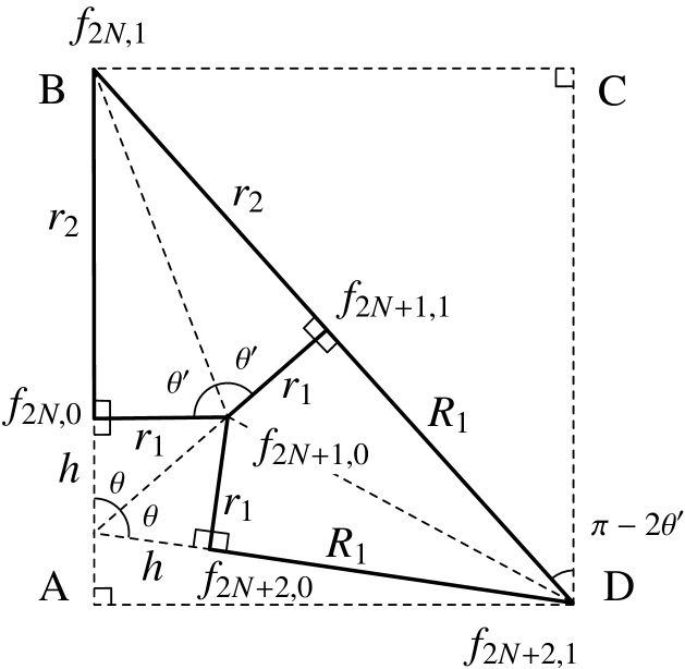
(ii) $-\pi<2\theta\leq-\frac{\pi}{2}$

Figure 11: Configuration of points in Lemma 5.6.

Then we have $h=\dfrac{r_{1}^{2}(r_{2}+R_{1})}{r_{2}R_{1}-r_{1}^{2}}$, and thus (5.37). Figure 11 (ii) illustrates the case of $-\pi<2\theta\leq-\pi/2$. We see from ${\rm AB}={\rm DC}$ that

$$(h+R_{1})\cos(\pi-|2\theta|)+h+r_{2}=(r_{2}+R_{1})\cos(\pi-2\theta^{\prime}),$$ (5.41)

which also leads us to (5.40), and thus (5.37). Therefore we have proved Lemma 5.6.  $\square$

From (5.32), (5.34) and the initial condition $f_{0,0}=0,\,f_{1,0}=1$, we see by induction that the points $f_{n,0}$ satisfy

$$\gamma f_{n,0}=2n\dfrac{(f_{n+1,0}-f_{n,0})(f_{n,0}-f_{n-1,0})}{f_{n+1,0}-f_{n-1,0}}.$$ (5.42)

Similarly, we see that $f_{0,m}$ satisfy

$$\gamma f_{0,m}=2m\dfrac{(f_{0,m+1}-f_{0,m})(f_{0,m}-f_{0,m-1})}{f_{0,m+1}-f_{0,m-1}}.$$ (5.43)

Thus it is possible to determine $f_{n,m}$ in $\mathbb{Z}_{+}^{2}$ by using (2.1). Since (2.1) is compatible with (2.3), $f_{n,m}$ satisfies (2.3) simultaneously. This proves the second part of Theorem 5.3.  $\square$

5.2 Positivity of radii of circles

Theorem 5.3 claims that if $R_{n,m}$ satisfying (5.13) and (5.14) is positive, then the corresponding $f_{n,m}$ is an immersion. In order to establish Theorem 5.1, we have to prove the positivity of $R_{n,m}$ determined by (5.13) and (5.14) with the initial condition $R_{1,0}=1$, $R_{0,1}=\zeta\,(>0)$. First, we show that positivity of $R_{m,n}$ for $(n,m)\in{\bf V}$ is reduced to that of $R_{n,n+1}$ for $n\in\mathbb{Z}_{+}$.

Proposition 5.7

Let the solution $R_{n,m}$ of (5.13) for $(n,m)\in{\bf V}$ and (5.14) for $n=m\in\mathbb{Z}_{+}$ with initial data

$$R_{1,0}=1,\quad R_{0,1}=\zeta\,(>0)$$ (5.44)

be positive for $m=n+1$, namely, $R_{n,n+1}>0$ for any $n\in\mathbb{Z}_{+}$. Then $R_{n,m}$ is positive everywhere in ${\bf V}$ and satisfies (5.14) for $(n,m)\in{\bf V}$.

Proof. Equation (5.14) for $(n,m)=(0,0)$ with initial data (5.44) determines $R_{1,2}$. We use (5.13) and (5.14) for $n=m$ inductively to get $R_{n,n+1}$ and $R_{n+1,n}$. As was mentioned before, we see that $R_{2n+1,0}=1$ and $R_{0,2m+1}=\zeta$ for all $n,m\in\mathbb{Z}_{+}$ by putting $n=0$ and $m=0$, respectively, in (5.13). With these data one can determine $R_{n,m}$ in ${\bf V}$ by using (5.13). When $n\geq m$, we use (5.13) in the form of

$$R_{n+1,m}=R_{n-1,m}\dfrac{(n-m)R_{n,m+1}+(n+m)R_{n,m-1}}{(n+m)R_{n,m+1}+(n-m)R_{n,m-1}}.$$ (5.45)

For positive $R_{n-1,m},R_{n,m+1}$ and $R_{n,m-1}$, we get $R_{n+1,m}>0$. When $m\geq n$, one can show in a similar way that $R_{n,m+1}>0$ for given positive $R_{n,m-1},R_{n+1,m}$ and $R_{n-1,m}$ by using (5.13). One can show by induction that we have (5.30) for $m=n\geq 1$, and we get (5.14) for $n=m+2$. Similarly, one can show by induction that we have (5.30) at $(n+2k,n)$ for $n,k\geq 1$, and (5.14) for $(n+2k,n)$. Thus we obtain (5.14) for $n\geq m$. One can show in a similar way that we have (5.14) for $n\leq m$ by using (5.30) at $(n,n+2k)$ as an auxiliary relation.   $\square$

Due to Proposition 5.7, the discrete function $Z^{\gamma}$ with ${\rm Re}~{}\gamma=1$ is an immersion if and only if $R_{n,n+1}>0$ for all $n\in\mathbb{Z}_{+}$. We next reduce the positivity to the existence of unitary solution to a certain system of difference equations.

Proposition 5.8

The map $f\,:\,\mathbb{Z}_{+}^{2}\to\mathbb{C}$ satisfying (2.1) and (2.3) with the initial condition $f_{0,0}=0,f_{1,0}=1,f_{0,1}=i\zeta\,(\zeta>0)$ is an immersion if and only if the solution $(x_{n},y_{n})$ to the system of equations

$$\begin{array}[]{l}(x_{n}-1)\dfrac{y_{n+1}-1}{x_{n}+y_{n+1}}+(x_{n}+1)\dfrac{y_{n}-1}{x_{n}y_{n}-1}=0,\\[11.38109pt] \dfrac{\gamma}{2}=\dfrac{n+2}{1-x_{n+1}^{-1}y_{n+1}^{-1}}-\dfrac{n+1}{1+x_{n}^{-1}y_{n+1}},\quad x_{0}y_{0}=\dfrac{\gamma}{\gamma-2},\end{array}$$ (5.46)

with

$$y_{0}=\dfrac{\zeta+i}{\zeta-i},$$ (5.47)

is of the form $x_{n}=e^{2i\alpha_{n}},y_{n}=e^{2i\varphi_{n}}$, where $\alpha_{n},\varphi_{n}\in(0,\pi/2)$.

Proof. Let $f_{n,m}$ be an immersion. Define $\alpha_{n},\varphi_{n}\in(0,\pi/2)$ through

$$f_{n,n+2}-f_{n,n+1}=e^{2i\alpha_{n}}(f_{n+1,n+1}-f_{n,n+1}),\quad f_{n+1,n+1}-f_{n,n+1}=e^{2i\varphi_{n}}(f_{n,n}-f_{n,n+1}).$$ (5.48)

Using Proposition 5.2, one obtains

$$\begin{array}[]{ll}f_{n+1,n+1}-f_{n,n+1}=R_{n,n+1}e^{i(2\varphi_{n}-\pi/2+\beta_{n})},&f_{n,n+1}-f_{n-1,n+1}=R_{n,n+1}e^{i(\beta_{n}+2\alpha_{n-1}-\pi/2)},\\[5.69054pt] f_{n,n+2}-f_{n,n+1}=R_{n,n+1}e^{i(2\varphi_{n}-\pi/2+2\alpha_{n}+\beta_{n})},&f_{n,n+1}-f_{n,n}=R_{n,n+1}e^{i(\beta_{n}+\pi/2)},\end{array}$$ (5.49)

where $\beta_{n}=\arg\,(f_{n+1,n}-f_{n,n})$. Figure 12 is a schematic diagram illustrating the configuration of the relevant quadrilaterals.

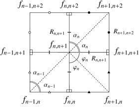
Figure 12: A schematic diagram of quadrilaterals for Proposition 5.8.

Now the constraint (2.3) for $(n,n+1)$ is equivalent to

$$\gamma f_{n,n+1}=-2iR_{n,n+1}e^{i\beta_{n}}\left(\dfrac{n}{e^{-2i\varphi_{n}}+e^{-2i\alpha_{n-1}}}+\dfrac{n+1}{e^{-2i(\varphi_{n}+\alpha_{n})}-1}\right).$$ (5.50)

Putting these expressions into the equality

$$f_{n+1,n+2}-f_{n,n+1}=e^{i(2\varphi_{n}-\pi/2+\beta_{n})}(R_{n,n+1}+iR_{n+1,n+2}),$$ (5.51)

together with $R_{n+1,n+2}=R_{n,n+1}\tan\alpha_{n}$ and $e^{i\beta_{n+1}}=e^{i(\beta_{n}-\pi/2+2\varphi_{n})}$, one obtains

$$\begin{array}[]{l}2i\sin\alpha_{n}\left(\dfrac{n+1}{e^{-2i\varphi_{n+1}}+e^{-2i\alpha_{n}}}+\dfrac{n+2}{e^{-2i(\varphi_{n+1}+\alpha_{n+1})}-1}\right)\\[11.38109pt] +2\cos\alpha_{n}\left(\dfrac{n}{1+e^{2i(\varphi_{n}-\alpha_{n-1})}}+\dfrac{n+1}{e^{-2i\alpha_{n}}-e^{2i\varphi_{n}}}\right)=-\gamma e^{i\alpha_{n}}.\end{array}$$ (5.52)

On the other hand, equation (5.14) for $m=n$ is reduced to

$$\delta R_{n,n+1}=(n+1)\dfrac{R_{n+1,n}R_{n+1,n+2}-R_{n,n+1}^{2}}{R_{n+1,n}+R_{n+1,n+2}}-n\dfrac{R_{n,n+1}^{2}-R_{n+1,n}R_{n-1,n}}{R_{n+1,n}+R_{n-1,n}}.$$ (5.53)

By a similar geometric consideration to the proof of Lemma 5.6, this implies

$$\delta=-(n+1)\cot(\alpha_{n}+\varphi_{n})-n\tan(\alpha_{n-1}-\varphi_{n}),$$ (5.54)

which can be transformed to

$$\dfrac{\gamma}{2}=\dfrac{n+1}{1-e^{-2i(\alpha_{n}+\varphi_{n})}}-\dfrac{n}{1+e^{2i(\varphi_{n}-\alpha_{n-1})}}.$$ (5.55)

By using (5.55), we see that (5.52) yields the first equation of (5.46) with $x_{n}=e^{2i\alpha_{n}}$ and $y_{n}=e^{2i\varphi_{n}}$. The second equations of (5.46) come from (5.55). This proves the necessity part.

Now let us suppose that there is a solution $(x_{n},y_{n})=(e^{2i\alpha_{n}},e^{2i\varphi_{n}})$ of (5.46) with $\alpha_{n},\varphi_{n}\in(0,\pi/2)$. This solution together with (5.48) and (2.1) determines a sequence of orthogonal circles with their centers on $f_{n,n+1}$, and thus the points $(f_{n,n+1},f_{n\pm 1,n+1},f_{n,n},f_{n,n+2})$. Now (2.1) determines $f_{n,m}$ on $\mathbb{Z}_{+}^{2}$. Since $\alpha_{n},\varphi_{n}\in(0,\pi/2)$, the inner parts of the quadrilaterals $(f_{n,n+1},f_{n+1,n+1},f_{n+1,n+2},f_{n,n+2})$ and of the quadrilaterals $(f_{n,n},f_{n+1,n},f_{n+1,n+1},f_{n,n+1})$ are disjoint, which means that we have positive solution $R_{n,n+1}$ and $R_{n+1,n}$ of (5.13) and (5.14). Given $R_{n+1,n}$ and $R_{n,n+1}$, (5.13) determines $R_{n,m}$ for all $(n,m)\in{\bf V}$. Due to Proposition 5.7, $R_{n,m}$ is positive, and satisfies (5.13) and (5.14). Theorem 5.3 implies that the discrete conformal map $g_{n,m}$ corresponding to the circle pattern $\{C_{n,m}\}$ determined by $R_{n,m}$ is an immersion and satisfies (2.3). Since $g_{n,n}=f_{n,n}$ and $g_{n,n\pm 1}=f_{n,n\pm 1}$, equation (2.1) implies $g_{n,m}=f_{n,m}$. This proves Proposition 5.8.   $\square$

Note that although (5.46) is a system of equations, a solution $(x_{n},y_{n})$ of (5.46) is determined by its initial value $y_{0}$.

The system of equation (5.46) can be written in the following recurrent form:

$$y_{n+1}=\dfrac{1+x_{n}^{2}-2x_{n}y_{n}}{x_{n}^{2}y_{n}+y_{n}-2x_{n}},\quad x_{n+1}=\dfrac{(2n+2+\gamma)x_{n}+\gamma y_{n+1}}{y_{n+1}\big{[}(\gamma-2)x_{n}+(\gamma-2n-4)y_{n+1}\big{]}},$$ (5.56)

or

$$y_{n+1}=\Phi(x_{n},y_{n}),\quad x_{n+1}=\Psi(n,x_{n},y_{n+1}),$$ (5.57)

$$\Phi(x,y)=y\dfrac{x^{-1}y^{-1}+xy^{-1}-2}{xy+x^{-1}y-2},\quad\Psi(n,x,y)=-\dfrac{1}{x}\dfrac{(2n+3+i\delta)xy^{-1}+(1+i\delta)}{(2n+3-i\delta)x^{-1}y+(1-i\delta)},$$ (5.58)

and $x_{0}=-\dfrac{1+i\delta}{1-i\delta}\dfrac{1}{y_{0}}$. It is easy to see that $|\Phi(x,y)|=|\Psi(n,x,y)|=1$ when $|x|=|y|=1$ and that $|x_{0}|=1$ when $|y_{0}|=1$, which implies that this system possesses unitary solutions. Moreover, we have the following theorem as for the arguments of the unitary solutions:

Theorem 5.9

There exists a unitary solution $(x_{n},y_{n})$ to the system of equation (5.46) with $x_{n},y_{n}\in A_{\rm I}\backslash\{\pm 1\}$, where

$$A_{\rm I}=\{e^{2i\beta}\,|\,\beta\in[0,\pi/2]\}.$$ (5.59)

Proof We first investigate the properties of the function $\Phi(x,y)$ and $\Psi(n,x,y)$ restricted to the torus $T^{2}=S^{1}\times S^{1}=\{(x,y)\,|\,x,y\in\mathbb{C},\,|x|=|y|=1\}$.

Property 1. The function $\Phi(x,y)$ is continuous on $A_{\rm I}\times A_{\rm I}\backslash\{(\pm 1,\pm 1)\}$. The function $\Psi(n,x,y)$ is continuous on $A_{\rm I}\times A_{\rm I}$ for any $n\in\mathbb{Z}_{+}$. (Continuity on the boundary of $A_{\rm I}\times A_{\rm I}$ is understood to be one-sided.)

The points of discontinuity must satisfy

$$x^{2}y+y-2x=0,\quad(2n+3-i\delta)y+(1-i\delta)x=0.$$ (5.60)

The first identity holds only for $(x,y)=(\pm 1,\pm 1)$. The second never holds for unitary $x,y$.

Property 2. For $(x,y)\in A_{\rm I}\times A_{\rm I}\backslash\{(\pm 1,\pm 1)\}$, we have $\Phi(x,y)\in A_{\rm I}$. For $(x,y)\in A_{\rm I}\times A_{\rm I}$, we have $\Psi(n,x,y)\in A_{\rm I}\cup A_{\rm II}\cup A_{\rm IV}$, where $A_{\rm II}:=\{e^{2i\beta}\,|\,\beta\in(\pi/2,\pi]\}$ and $A_{\rm IV}:=\{e^{2i\beta}\,|\,\beta\in[-\pi/2,0)\}$.

Property 2 is verified as follows: using the transformation

$$u_{n}=\tan\alpha_{n},\quad v_{n}=\tan\varphi_{n},$$ (5.61)

where $x_{n}=e^{2i\alpha_{n}}$and $y_{n}=e^{2i\varphi_{n}}$, we see that the first equation of (5.46) takes the form

$$v_{n+1}=u_{n}^{-2}v_{n}.$$ (5.62)

It is obvious that $u^{-2}v\in[0,+\infty]$ when $(u,v)\in[0,+\infty]\times[0,+\infty]\backslash\{(0,0),(+\infty,+\infty)\}$. The second equation of (5.46) can be expressed as

$$\alpha_{n+1}=\omega_{n}-\alpha_{n}+\dfrac{\pi}{2},\quad e^{2i\omega_{n}}=\dfrac{(2n+3+i\delta)x_{n}y_{n+1}^{-1}+(1+i\delta)}{(2n+3-i\delta)x_{n}^{-1}y_{n+1}+(1-i\delta)}.$$ (5.63)

By using the variables $u_{n},v_{n+1}$, we have

$$\tan(\omega_{n}-\alpha_{n})=F(n,u_{n},v_{n+1}),$$ (5.64)

where

$$F(n,u,v)=\dfrac{[(n+1)-(n+2)v^{2}]u-(2n+3)v+\delta(1+uv)}{(n+2)-(n+1)v^{2}+(2n+3)uv+\delta v(1+uv)}.$$ (5.65)

Lemma 5.10

It holds that $\omega_{n}-\alpha_{n}+\frac{\pi}{2}\in[-\pi/2,\pi]$ for $\alpha_{n},\varphi_{n+1}\in[0,\pi/2]$.

Proof. Let us investigate the function $F(n,u,v)$ for $u,v\in[0,+\infty]$. It is easy to see that

$$\dfrac{\partial F(n,u,v)}{\partial u}>0,\quad\dfrac{\partial F(n,u,v)}{\partial v}<0$$ (5.66)

on $[0,+\infty]^{2}$ except for the points satisfying $(n+2)-(n+1)v^{2}+(2n+3)uv+\delta v(1+uv)=0$. Consider the values of $F(n,u,v)$ on the boundary of $[0,+\infty]^{2}$. It is easy to see that

$$F(n,0,+\infty)=0,\quad F(n,0,0)=\dfrac{\delta}{n+2},\quad F(n,+\infty,+\infty)=-\dfrac{n+2}{\delta},\quad F(n,+\infty,0)=+\infty.$$ (5.67)

We find that $\dfrac{dF(n,0,v)}{dv}<0$ except for the point $v=v_{+}:=\dfrac{\delta+\sqrt{\delta^{2}+4(n+1)(n+2)}}{2(n+1)}$, and that $F(n,u,0)=\dfrac{(n+1)u+\delta}{n+2}$ is monotone increasing. Note that

$$F(n,u,+\infty)=\dfrac{(n+2)u}{n+1-\delta u},\quad F(n,+\infty,v)=\dfrac{-(n+2)v^{2}+\delta v+n+1}{v(\delta v+2n+3)}.$$ (5.68)

When $\delta>0$, we see that $\dfrac{dF(n,u,+\infty)}{du}>0$ except for the point $u=\dfrac{n+1}{\delta}$ and that $\dfrac{dF(n,+\infty,v)}{dv}<0$ except for the point $v=0$. When $\delta<0$, we see that $\dfrac{dF(n,u,+\infty)}{du}>0$ and that $\dfrac{dF(n,+\infty,v)}{dv}<0$ except for the points $v=0,v_{*}:=-\dfrac{2n+3}{\delta}$. The singular points of $F(n,u,v)$ can be expressed by $(u,v)=(G(v),v)$, where $G(v)=\dfrac{(n+1)v^{2}-\delta v-(n+2)}{v(\delta v+2n+3)}$, if $v\neq 0,v_{*}$. Note that $(u,v)\in[0,+\infty]^{2}$. Then we find that the singular points lie in $v\in[v_{+},+\infty],u\in[0,(n+1)/\delta]$ (when $\delta>0$) or in $v\in[v_{+},v_{*}],u\in[0,+\infty]$ (when $\delta<0$), and that $G(v)$ is monotone increasing (See Figure 13). Therefore we see that $\omega_{n}-\alpha_{n}\in[-\pi,\pi/2]$ when $\alpha_{n},\varphi_{n+1}\in[0,\pi/2]$.   $\square$

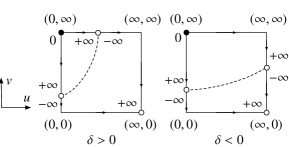
Figure 13: Behaviour of $F(n,u,v)$.

The final equation in (5.46) leads us to

$$\alpha_{0}=-\varphi_{0}+\theta+\dfrac{\pi}{2},\quad\tan\theta=\delta.$$ (5.69)

It is easy to see that $-\varphi_{0}+\theta+\pi/2\in[-\pi/2,\pi]$ when $\varphi_{0}\in(0,\pi/2)$. Therefore property 2 is established.

Now let us introduce

$$\begin{array}[]{l}S_{\rm II}(k):=\{y_{0}\in A_{\rm I}\,|\,x_{k}\in A_{\rm II},\,x_{l}\in A_{\rm I}\,(l<k)\},\\[2.84526pt] S_{\rm IV}(k):=\{y_{0}\in A_{\rm I}\,|\,x_{k}\in A_{\rm IV},\,x_{l}\in A_{\rm I}\,(l<k)\},\end{array}$$ (5.70)

where $(x_{n},y_{n})$ is the solution of (5.46). From property 1, it follows that $S_{\rm II}(k)$ and $S_{\rm IV}(k)$ are open sets in the induced topology of $A_{\rm I}$. Denote

$$S_{\rm II}=\cup S_{\rm II}(k),\quad S_{\rm IV}=\cup S_{\rm IV}(k),$$ (5.71)

which are also open. These sets are nonempty since $S_{\rm II}(1)$ and $S_{\rm IV}(1)$ are nonempty (See the proof of Lemma 5.10). Note that $S_{\rm II}(0)$ or $S_{\rm IV}(0)$ can be empty. Finally, introduce

$$S_{\rm I}:=\{y_{0}\in A_{\rm I}\,|\,x_{n}\in A_{\rm I}\,\,\mbox{for all}\,\,n\in\mathbb{Z}_{+}\}.$$ (5.72)

It is obvious that $S_{\rm I},S_{\rm II}$ and $S_{\rm IV}$ are mutually disjoint. Property 2 implies

$$S_{\rm I}\cup S_{\rm II}\cup S_{\rm IV}=A_{\rm I}.$$ (5.73)

Since the connected set $A_{\rm I}$ cannot be covered by two open disjoint subsets $S_{\rm II}$ and $S_{\rm IV}$, we see that $S_{\rm I}\neq\emptyset$. So there exists $y_{0}$ such that the solution $(x_{n},y_{n})\in A_{\rm I}\times A_{\rm I}$ for any $n\in\mathbb{Z}_{+}$. Suppose that $\alpha_{n}=0,\varphi_{n}\neq 0$ hold at a certain $n$. Then we get $\varphi_{n+1}=\pi/2$ and $\alpha_{n+1}=-\pi/2$ from (5.56), or (5.62) and (5.63). Similarly, if $\alpha_{n}=\pi/2,\varphi_{n}\neq\pi/2$ hold at a certain $n$, we get $\varphi_{n+1}=0$ and then $\alpha_{n+1}=\pi$. It means that in both cases $x_{n+1}\not\in A_{\rm I}$. Suppose that $\varphi_{n}\neq 0,\varphi_{n+1}=0$ hold at a certain $n$. Then we get $\alpha_{n}=\pi/2$ and then $\alpha_{n+1}=\pi$ from (5.56), or (5.62) and (5.63). Similarly, if $\varphi_{n}\neq\pi/2,\varphi_{n+1}=\pi/2$ hold at a certain $n$, we get $\alpha_{n}=0$ and then $\alpha_{n+1}=-\pi/2$. It also means that in both cases $x_{n+1}\not\in A_{\rm I}$. Thus, it follows that $\alpha_{n}\neq 0,\pi/2$ and $\varphi_{n}\neq 0,\pi/2$ for the solution $(x_{n},y_{n})\in A_{\rm I}\times A_{\rm I}$ for any $n\in\mathbb{Z}_{+}$.   $\square$

We have shown that $S_{\rm I}$ is not empty. In order to establish Theorem 5.1, let us finally show the uniqueness of the initial condition which gives rise to the solution $(x_{n},y_{n})\in A_{\rm I}\times A_{\rm I}\backslash\{(\pm 1,\pm 1)\}$, namely, the circle pattern. Indeed, the initial condition is nothing but that for the discrete power function. Take a solution $(x_{n},y_{n})$ such that $y_{0}\in S_{\rm I}$ and consider the corresponding circle pattern. Let $R_{k}$ be radii of circles with centers at $f_{2k,1}$, i.e., $R_{k}:=R_{2k,1}$. We have the following lemma.

Lemma 5.11

An explicit formula for $R_{k}$ is given by

$$R_{k}=i\,\dfrac{(-1)^{k}\left[\left(\frac{r-k+1}{2}\right)_{k}-\left(\frac{r-k}{2}\right)_{k}\right]-i\zeta\left[\left(\frac{r-k+1}{2}\right)_{k}+\left(\frac{r-k}{2}\right)_{k}\right]}{(-1)^{k}\left[\left(\frac{r-k+1}{2}\right)_{k}+\left(\frac{r-k}{2}\right)_{k}\right]-i\zeta\left[\left(\frac{r-k+1}{2}\right)_{k}-\left(\frac{r-k}{2}\right)_{k}\right]},$$ (5.74)

where $\zeta=R_{0}$.

Proof The radii $R_{k}$ are defined by $R_{k}=|f_{2k,0}-f_{2k,1}|=|v_{2k,0}||v_{2k,1}|$ (see (2.8)). From Proposition 3.2, we have

$$v_{2k,0}=\dfrac{(r)_{k}}{(-r+1)_{k}},\quad v_{2k,1}=\dfrac{\varphi(-k+1,-r-k+1,-r+2;-1)}{\varphi(-k,-r-k+1,-r+1;-1)},$$ (5.75)

where $\varphi(a,b,c;-1)$ is given by (see (2.15))

$$\begin{split}\varphi(a,b,c;-1)&=\dfrac{\Gamma(a)\Gamma(b)}{\Gamma(c)}F(a,b,c;-1)\\ &+c_{1}e^{\pi i(1-c)}\dfrac{\Gamma(a-c+1)\Gamma(b-c+1)}{\Gamma(2-c)}F(a-c+1,b-c+1,2-c;-1),\end{split}$$ (5.76)

and

$$\zeta=c_{1}e^{-\pi\delta/2}\,(>0).$$ (5.77)

It is easy to see that $|v_{2k,0}|=1$ under ${\rm Re}\,\gamma=1$. Due to the formulae [1]

$$F(a,b,a-b+1;-1)=2^{-a}\pi^{1/2}\dfrac{\Gamma(a-b+1)}{\Gamma(\frac{1}{2}a-b+1)\Gamma(\frac{1}{2}a+\frac{1}{2})},$$ (5.78)

$$\begin{split}&F(a,b,a-b+2;-1)=2^{-a}\pi^{1/2}(b-1)^{-1}\Gamma(a-b+2)\\ &\hskip 113.81102pt\times\left[\dfrac{1}{\Gamma(\frac{1}{2}a)\Gamma(\frac{1}{2}a-b+\frac{3}{2})}-\dfrac{1}{\Gamma(\frac{1}{2}a+\frac{1}{2})\Gamma(\frac{1}{2}a-b+1)}\right],\end{split}$$ (5.79)

and the contiguity relation

$$\begin{split}&(c-a)(c-b)tF(a,b,c+1;t)+c\left[(a+b-2c+1)t+c-1\right]F(a,b,c;t)\\ &\hskip 113.81102pt+c(c-1)(t-1)F(a,b,c-1;t)=0,\end{split}$$ (5.80)

we get

$$v_{2k,1}=\dfrac{(-1)^{k}\left[\left(\frac{r-k+1}{2}\right)_{k}-\left(\frac{r-k}{2}\right)_{k}\right]-i\zeta\left[\left(\frac{r-k+1}{2}\right)_{k}+\left(\frac{r-k}{2}\right)_{k}\right]}{(-1)^{k}\left[\left(\frac{r-k+1}{2}\right)_{k}+\left(\frac{r-k}{2}\right)_{k}\right]-i\zeta\left[\left(\frac{r-k+1}{2}\right)_{k}-\left(\frac{r-k}{2}\right)_{k}\right]}.$$ (5.81)

Then we can easily verify that $v_{2k,1}$ satisfy the recurrence relation

$$v_{2(k+1),1}=-\dfrac{1-i\varepsilon_{k}v_{2k,1}}{v_{2k,1}-i\varepsilon_{k}},\quad v_{0,1}=-i\zeta,$$ (5.82)

where $\varepsilon_{k}=\dfrac{\delta}{2k+1}$. On the other hand, (5.26) for $m=0$ is reduced to

$$R_{k+1}=\dfrac{1-\varepsilon_{k}R_{k}}{R_{k}+\varepsilon_{k}}.$$ (5.83)

Then noticing $R_{0}=\zeta$, we see that $R_{k}=|v_{2k,1}|=iv_{2k,1}$.   $\square$

Proposition 5.12

The set $S_{\rm I}$ consists of only one element $\dfrac{e^{-\pi\delta/2}+i}{e^{-\pi\delta/2}-i}$.

Proof By using the formulae

$$\Gamma(z)\Gamma(1-z)=\dfrac{\pi}{\sin\pi z},$$ (5.84)

and the asymptotic formula as $z\to\infty$

$$\Gamma(az+b)\sim(2\pi)^{1/2}e^{-az}(az)^{az+b-\frac{1}{2}}\quad(|\arg z|<\pi\,,\ a>0),$$ (5.85)

we get

$$\lim_{l\to\infty}R_{2l}=\dfrac{(1-e^{-\pi\delta/2})+\zeta(1+e^{-\pi\delta/2})}{(1+e^{-\pi\delta/2})-\zeta(1-e^{-\pi\delta/2})},\quad\lim_{l\to\infty}R_{2l-1}=\dfrac{(1+e^{-\pi\delta/2})-\zeta(1-e^{-\pi\delta/2})}{(1-e^{-\pi\delta/2})+\zeta(1+e^{-\pi\delta/2})}.$$ (5.86)

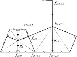
Figure 14: Configuration of points around $f_{2k,0}$ for large $k$.

The relation (5.34) implies $\displaystyle\lim_{N\to\infty}\theta_{N}=0$. Figure 14 illustrates the configuration around $f_{2k,0}$ for sufficiently large $k$. Note that the three points $f_{2k,0}$, $f_{2k+1,0}$, $f_{2k+2,0}$ are asymptotically collinear. We see from (5.86) that $R_{k}$ should behave as $\displaystyle\lim_{k\to\infty}R_{k}=1$ irrespective of the parity of $k$, since the four points $f_{2k+1,1},f_{2k+2,1},f_{2k+2,2},f_{2k+1,2}$ form a quadrilateral. Then we find that $\zeta=e^{-\pi\delta/2}$. This completes the proof of Proposition 5.12.   $\square$

Therefore $f_{n,m}$ satisfying (2.1) and (2.3) is an immersion if and only if the initial condition is given by (5.1). This completes the proof of Theorem 5.1.

6 Concluding remarks

The discrete logarithmic function and cases where $\gamma\in 2\mathbb{Z}$ were excluded from the considerations in the previous sections. From the viewpoint of the theory of hypergeometric functions, these cases lead to integer differences in the characteristic exponents. Thus we need a different treatment for the precise description of these cases. However, they may be obtained by some limiting procedures in principle. In fact, Agafonov has examined the case where $\gamma=2$ and $\gamma=0$ by using a limiting procedure [2, 3], the former is the discrete power function $Z^{2}$ and latter is the discrete logarithmic function. In general, one may obtain a description of these cases by introducing the functions $\widetilde{f}_{n,m}$ and $\widehat{f}_{n,m}$ as

$$\widetilde{f}_{n,m}:=\left\{\begin{array}[]{ll}\displaystyle\lim_{r\to j}\dfrac{1}{j}\dfrac{(-r+1)_{j}}{(r+1)_{j-1}}f_{n,m},&\mbox{for $\gamma=2j\in 2\mathbb{Z}_{>0}$}\\[11.38109pt] \displaystyle\lim_{r\to-j}\dfrac{(-r+1)_{j}}{(r+1)_{j}}f_{n,m},&\mbox{for $\gamma=-2j\in 2\mathbb{Z}_{<0}$}\end{array}\right.$$ (6.1)

and

$$\widehat{f}_{n,m}=\lim_{r\to 0}\dfrac{f_{n,m}-1}{r},$$ (6.2)

respectively. The function $\widetilde{f}_{n,m}$ might coincide with the counterpart defined in section 6 of [4].

Moreover, it has been shown that the discrete power function and logarithmic function associated with hexagonal patterns are also described by some discrete Painlevé equations [5]. It may be an interesting problem to construct the explicit formula for them.

Appendix A Bäcklund transformations of the sixth Painlevé equation

As a preparation, we give a brief review of the Bäcklund transformations and some of the bilinear equations for the $\tau$ functions [13]. It is well-known that P_VI (2.12) is equivalent to the Hamilton system

$$q^{\prime}=\dfrac{\partial H}{\partial p},\quad p^{\prime}=-\dfrac{\partial H}{\partial q},\quad^{\prime}=t(t-1)\dfrac{d}{dt},$$ (A.1)

whose Hamiltonian is given by

$$H=f_{0}f_{3}f_{4}f_{2}^{2}-[\alpha_{4}f_{0}f_{3}+\alpha_{3}f_{0}f_{4}+(\alpha_{0}-1)f_{3}f_{4}]f_{2}+\alpha_{2}(\alpha_{1}+\alpha_{2})f_{0}.$$ (A.2)

Here $f_{i}$ and $\alpha_{i}$ are defined by

$$f_{0}=q-t,\quad f_{3}=q-1,\quad f_{4}=q,\quad f_{2}=p,$$ (A.3)

and

$$\alpha_{0}=\theta,\quad\alpha_{1}=\kappa_{\infty},\quad\alpha_{3}=\kappa_{1},\quad\alpha_{4}=\kappa_{0}$$ (A.4)

with $\alpha_{0}+\alpha_{1}+2\alpha_{2}+\alpha_{3}+\alpha_{4}=1$. The Bäcklund transformations of P_VI are described by

$$s_{i}(\alpha_{j})=\alpha_{j}-a_{ij}\alpha_{i}\quad(i,j=0,1,2,3,4),$$ (A.5)

$$s_{2}(f_{i})=f_{i}+\dfrac{\alpha_{2}}{f_{2}},\quad s_{i}(f_{2})=f_{2}-\dfrac{\alpha_{i}}{f_{i}}~{}~{}(i=0,3,4),$$ (A.6)

$$\begin{array}[]{ll}s_{5}:&\alpha_{0}\leftrightarrow\alpha_{1},\quad\alpha_{3}\leftrightarrow\alpha_{4},\quad f_{2}\mapsto-\dfrac{f_{0}(f_{2}f_{0}+\alpha_{2})}{t(t-1)},\quad f_{4}\mapsto t\dfrac{f_{3}}{f_{0}},\\[11.38109pt] s_{6}:&\alpha_{0}\leftrightarrow\alpha_{3},\quad\alpha_{1}\leftrightarrow\alpha_{4},\quad f_{2}\mapsto-\dfrac{f_{4}(f_{4}f_{2}+\alpha_{2})}{t},\quad f_{4}\mapsto\dfrac{t}{f_{4}},\\[11.38109pt] s_{7}:&\alpha_{0}\leftrightarrow\alpha_{4},\quad\alpha_{1}\leftrightarrow\alpha_{3},\quad f_{2}\mapsto\dfrac{f_{3}(f_{3}f_{2}+\alpha_{2})}{t-1},\quad f_{4}\mapsto\dfrac{f_{0}}{f_{3}},\end{array}$$ (A.7)

where $A=(a_{ij})_{i,j=0}^{4}$ is the Cartan matrix of type $D^{(1)}_{4}$. Then the group of birational transformations $\langle s_{0},\ldots,s_{7}\rangle$ generate the extended affine Weyl group $\widetilde{W}(D^{(1)}_{4})$. In fact, these generators satisfy the fundamental relations

$$s_{i}^{2}=1\quad(i=0,\ldots,7),\quad s_{i}s_{2}s_{i}=s_{2}s_{i}s_{2}\quad(i=0,1,3,4),$$ (A.8)

and

$$\begin{array}[]{c}s_{5}s_{\{0,1,2,3,4\}}=s_{\{1,0,2,4,3\}}s_{5},\quad s_{6}s_{\{0,1,2,3,4\}}=s_{\{3,4,2,0,1\}}s_{6},\quad s_{7}s_{\{0,1,2,3,4\}}=s_{\{4,3,2,1,0\}}s_{7},\\[2.84526pt] s_{5}s_{6}=s_{6}s_{5},\quad s_{5}s_{7}=s_{7}s_{5},\quad s_{6}s_{7}=s_{7}s_{6}.\end{array}$$ (A.9)

We add a correction term to the Hamiltonian $H$ as follows,

$$H_{0}=H+\dfrac{t}{4}\left[1+4\alpha_{1}\alpha_{2}+4\alpha_{2}^{2}-(\alpha_{3}+\alpha_{4})^{2}\right]+\dfrac{1}{4}\left[(\alpha_{1}+\alpha_{4})^{2}+(\alpha_{3}+\alpha_{4})^{2}+4\alpha_{2}\alpha_{4}\right].$$ (A.10)

This modification gives a simpler behavior of the Hamiltonian with respect to the Bäcklund transformations. From the corrected Hamiltonian, we introduce a family of Hamiltonians $h_{i}~{}(i=0,1,2,3,4)$ as

$$h_{0}=H_{0}+\frac{t}{4},\quad h_{1}=s_{5}(H_{0})-\frac{t-1}{4},\quad h_{3}=s_{6}(H_{0})+\frac{1}{4},\quad h_{4}=s_{7}(H_{0}),\quad h_{2}=h_{1}+s_{1}(h_{1}).$$ (A.11)

Next, we also introduce $\tau$ functions $\tau_{i}~{}(i=0,1,2,3,4)$ by $h_{i}=(\log\tau_{i})^{\prime}$. Imposing the condition that the action of the $s_{i}$’s on the $\tau$ functions also commute with the derivation ^′, one can lift the Bäcklund transformations to the $\tau$ functions. The action of $\widetilde{W}(D^{(1)}_{4})$ is given by

$$s_{0}(\tau_{0})=f_{0}\dfrac{\tau_{2}}{\tau_{0}},\quad s_{1}(\tau_{1})=\dfrac{\tau_{2}}{\tau_{1}},\quad s_{2}(\tau_{2})=\dfrac{f_{2}}{\sqrt{t}}\dfrac{\tau_{0}\tau_{1}\tau_{3}\tau_{4}}{\tau_{2}},\quad s_{3}(\tau_{3})=f_{3}\dfrac{\tau_{2}}{\tau_{3}},\quad s_{4}(\tau_{4})=f_{4}\dfrac{\tau_{2}}{\tau_{4}},$$ (A.12)

and

$$\begin{array}[]{ll}s_{5}:&\tau_{0}\mapsto[t(t-1)]^{\frac{1}{4}}\tau_{1},\quad\tau_{1}\mapsto[t(t-1)]^{-\frac{1}{4}}\tau_{0},\\[2.84526pt] &\tau_{3}\mapsto t^{-\frac{1}{4}}(t-1)^{\frac{1}{4}}\tau_{4},\quad\tau_{4}\mapsto t^{\frac{1}{4}}(t-1)^{-\frac{1}{4}}\tau_{3},\quad\tau_{2}\mapsto[t(t-1)]^{-\frac{1}{2}}f_{0}\tau_{2},\end{array}$$ (A.13)

$$s_{6}:~{}\tau_{0}\mapsto it^{\frac{1}{4}}\tau_{3},\quad\tau_{3}\mapsto-it^{-\frac{1}{4}}\tau_{0},\quad\tau_{1}\mapsto t^{-\frac{1}{4}}\tau_{4},\quad\tau_{4}\mapsto t^{\frac{1}{4}}\tau_{1},\quad\tau_{2}\mapsto t^{-\frac{1}{2}}f_{4}\tau_{2},$$ (A.14)

$$\begin{array}[]{ll}s_{7}:&\tau_{0}\mapsto(-1)^{-\frac{3}{4}}(t-1)^{\frac{1}{4}}\tau_{4},\quad\tau_{4}\mapsto(-1)^{\frac{3}{4}}(t-1)^{-\frac{1}{4}}\tau_{0},\\[2.84526pt] &\tau_{1}\mapsto(-1)^{\frac{3}{4}}(t-1)^{-\frac{1}{4}}\tau_{3},\quad\tau_{3}\mapsto(-1)^{-\frac{3}{4}}(t-1)^{\frac{1}{4}}\tau_{1},\\[2.84526pt] &\tau_{2}\mapsto-i(t-1)^{-\frac{1}{2}}f_{3}\tau_{2}.\end{array}$$ (A.15)

We note that some of the fundamental relations are modified

$$s_{i}s_{2}(\tau_{2})=-s_{2}s_{i}(\tau_{2})\quad(i=5,6,7),$$ (A.16)

and

$$\begin{array}[]{l}s_{5}s_{6}\tau_{\{0,1,2,3,4\}}=\{i,-i,-1,-i,i\}s_{6}s_{5}\tau_{\{0,1,2,3,4\}},\\[2.84526pt] s_{5}s_{7}\tau_{\{0,1,2,3,4\}}=\{i,-i,-1,i,-i\}s_{7}s_{5}\tau_{\{0,1,2,3,4\}},\\[2.84526pt] s_{6}s_{7}\tau_{\{0,1,2,3,4\}}=\{-i,-i,-1,i,i\}s_{7}s_{6}\tau_{\{0,1,2,3,4\}}.\end{array}$$ (A.17)

Let us introduce the translation operators

$$\begin{array}[]{c}\widehat{T}_{13}=s_{1}s_{2}s_{0}s_{4}s_{2}s_{1}s_{7},\quad\widehat{T}_{40}=s_{4}s_{2}s_{1}s_{3}s_{2}s_{4}s_{7},\\ \widehat{T}_{34}=s_{3}s_{2}s_{0}s_{1}s_{2}s_{3}s_{5},\quad T_{14}=s_{1}s_{4}s_{2}s_{0}s_{3}s_{2}s_{6},\end{array}$$ (A.18)

whose action on the parameters $\vec{\alpha}=(\alpha_{0},\alpha_{1},\alpha_{2},\alpha_{3},\alpha_{4})$ is given by

$$\begin{array}[]{c}\widehat{T}_{13}(\vec{\alpha})=\vec{\alpha}+(0,1,0,-1,0),\\[2.84526pt] \widehat{T}_{40}(\vec{\alpha})=\vec{\alpha}+(-1,0,0,0,1),\\[2.84526pt] \widehat{T}_{34}(\vec{\alpha})=\vec{\alpha}+(0,0,0,1,-1),\\[2.84526pt] T_{14}(\vec{\alpha})=\vec{\alpha}+(0,1,-1,0,1).\end{array}$$ (A.19)

We denote $\tau_{k,l,m,n^{\prime}}=T_{14}^{n^{\prime}}\widehat{T}_{34}^{m}\widehat{T}_{40}^{l}\widehat{T}_{13}^{k}(\tau_{0})\,(k,l,m,n^{\prime}\in\mathbb{Z})$. By using this notation, we have

$$\begin{array}[]{ll}\tau_{0,0,0,0}=\tau_{0},&\tau_{-1,-1,-1,0}=[t(t-1)]^{\frac{1}{4}}\tau_{1},\\[2.84526pt] \tau_{0,-1,-1,0}=(-1)^{-\frac{3}{4}}t^{\frac{1}{4}}\tau_{3},&\tau_{0,-1,0,0}=(-1)^{-\frac{3}{4}}(t-1)^{\frac{1}{4}}\tau_{4},\\[2.84526pt] \tau_{-1,-2,-1,1}=(-1)^{-\frac{1}{4}}s_{0}(\tau_{0}),&\tau_{0,-1,0,1}=(-1)^{-\frac{3}{4}}[t(t-1)]^{\frac{1}{4}}s_{1}(\tau_{1}),\\[2.84526pt] \tau_{-1,-1,0,1}=-it^{\frac{1}{4}}s_{3}(\tau_{3}),&\tau_{-1,-1,-1,1}=(t-1)^{\frac{1}{4}}s_{4}(\tau_{4}),\end{array}$$ (A.20)

for instance. When the parameters $\vec{\alpha}$ take the values

$$(\alpha_{0},\alpha_{1},\alpha_{2},\alpha_{3},\alpha_{4})=(-b,a+n^{\prime},-n^{\prime},c-a,b-c+1+n^{\prime}),$$ (A.21)

the function $\tau_{k,l,m,n^{\prime}}$ relates to the hypergeometric $\tau$ function $\tau_{n^{\prime}}^{k,l,m}$ introduced in Proposition 2.6 by [13]

$$\tau_{k,l,m,n^{\prime}}=\omega_{k,l,m,n^{\prime}}\tau_{n^{\prime}}^{k,l,m}t^{-(\hat{a}+\hat{b}-\hat{c}+2n^{\prime})^{2}/4-(\hat{a}-\hat{b}-n^{\prime})^{2}/4+n^{\prime}(\hat{b}+n^{\prime})-n^{\prime}(n^{\prime}-1)/2}(t-1)^{(\hat{a}+\hat{b}-\hat{c}+2n^{\prime})^{2}/4+1/2},$$ (A.22)

where we denote $\hat{a}=a+k,\hat{b}=b+l+1$ and $\hat{c}=c+m$, and the constants $\omega_{k,l,m,n^{\prime}}=\omega_{k,l,m,n^{\prime}}(a,b,c)$ are determined by the recurrence relations

$$\begin{array}[]{l}\omega_{k+1,l,m,i}\omega_{k-1,l,m,i}=i\hat{a}(\hat{c}-\hat{a})\omega_{k,l,m,i}^{2},\\[2.84526pt] \omega_{k,l+1,m,i}\omega_{k,l-1,m,i}=-i\hat{b}(\hat{c}-\hat{b})\omega_{k,l,m,i}^{2},\\[2.84526pt] \omega_{k,l,m+1,i}\omega_{k,l,m-1,i}=(\hat{c}-\hat{a})(\hat{c}-\hat{b})\omega_{k,l,m,i}^{2}\end{array}\quad(i=0,1)$$ (A.23)

and

$$\omega_{k,l,m,n^{\prime}+1}\omega_{k,l,m,n^{\prime}-1}=-\omega_{k,l,m,n^{\prime}}^{2}$$ (A.24)

with initial conditions

$$\begin{array}[]{ll}\omega_{-1,-2,-1,1}=(-1)^{-1/4}b,&\omega_{0,-2,-1,1}=b,\\ \omega_{-1,-1,-1,1}=1,&\omega_{0,-1,-1,1}=(-1)^{-1/4},\\ \omega_{-1,0,0,1}=-(-1)^{-3/4}(c-a),&\omega_{0,0,0,1}=-i,\\ \omega_{-1,-1,0,1}=-i(c-a),&\omega_{0,-1,0,1}=(-1)^{-3/4},\end{array}$$ (A.25)

and

$$\begin{array}[]{ll}\omega_{-1,-2,-1,0}=(-1)^{-3/4}b,&\omega_{0,-2,-1,0}=-b,\\ \omega_{-1,-1,-1,0}=1,&\omega_{0,-1,-1,0}=(-1)^{-3/4},\\ \omega_{-1,0,0,0}=(-1)^{-3/4}(c-a),&\omega_{0,0,0,0}=1,\\ \omega_{-1,-1,0,0}=c-a,&\omega_{0,-1,0,0}=(-1)^{-3/4}.\end{array}$$ (A.26)

From the above formulation, one can obtain the bilinear equations for the $\tau$ functions. For example, let us express the Bäcklund transformations $s_{2}(f_{i})=f_{i}+\dfrac{\alpha_{2}}{f_{2}}\,(i=0,3,4)$ in terms of the $\tau$ functions $\tau_{j}\,(j=0,1,3,4)$. We have by using (A.12)

$$\begin{array}[]{l}\alpha_{2}t^{-\frac{1}{2}}\tau_{3}\tau_{4}-s_{1}(\tau_{1})s_{2}s_{0}(\tau_{0})+s_{0}(\tau_{0})s_{2}s_{1}(\tau_{1})=0,\\[2.84526pt] \alpha_{2}t^{-\frac{1}{2}}\tau_{0}\tau_{4}-s_{1}(\tau_{1})s_{2}s_{3}(\tau_{3})+s_{3}(\tau_{3})s_{2}s_{1}(\tau_{1})=0,\\[2.84526pt] \alpha_{2}t^{-\frac{1}{2}}\tau_{0}\tau_{3}-s_{1}(\tau_{1})s_{2}s_{4}(\tau_{4})+s_{4}(\tau_{4})s_{2}s_{1}(\tau_{1})=0.\end{array}$$ (A.27)

Applying the affine Weyl group $\widetilde{W}(D_{4}^{(1)})$ on these equations, we obtain

$$\begin{array}[]{l}(\alpha_{0}+\alpha_{2}+\alpha_{4})\,t^{-\frac{1}{2}}\tau_{3}s_{4}(\tau_{4})-s_{1}(\tau_{1})s_{4}s_{2}s_{0}(\tau_{0})+\tau_{0}s_{0}s_{4}s_{2}s_{1}(\tau_{1})=0,\\[2.84526pt] (\alpha_{0}+\alpha_{2}+\alpha_{4})\,t^{\frac{1}{2}}\tau_{1}\tau_{3}-\tau_{4}s_{4}s_{2}s_{0}(\tau_{0})+\tau_{0}s_{0}s_{2}s_{4}(\tau_{4})=0,\end{array}$$ (A.28)

$$\begin{array}[]{l}(\alpha_{0}+\alpha_{1}+\alpha_{2})\,t^{-\frac{1}{2}}\tau_{3}\tau_{4}-\tau_{1}s_{1}s_{2}s_{0}(\tau_{0})+\tau_{0}s_{0}s_{2}s_{1}(\tau_{1})=0,\\[2.84526pt] (\alpha_{0}+\alpha_{1}+\alpha_{2})\,t^{\frac{1}{2}}s_{1}(\tau_{1})\tau_{3}-s_{4}(\tau_{4})s_{1}s_{2}s_{0}(\tau_{0})+\tau_{0}s_{0}s_{1}s_{2}s_{4}(\tau_{4})=0,\end{array}$$ (A.29)

$$\begin{array}[]{l}(\alpha_{2}+\alpha_{3}+\alpha_{4})\,t^{-\frac{1}{2}}\tau_{0}\tau_{1}-\tau_{4}s_{4}s_{2}s_{3}(\tau_{3})+\tau_{3}s_{3}s_{2}s_{4}(\tau_{4})=0,\\[2.84526pt] (\alpha_{2}+\alpha_{3}+\alpha_{4})\,t^{-\frac{1}{2}}s_{4}(\tau_{4})\tau_{0}-s_{1}(\tau_{1})s_{4}s_{2}s_{3}(\tau_{3})+\tau_{3}s_{3}s_{4}s_{2}s_{1}(\tau_{1})=0,\end{array}$$ (A.30)

and

$$\begin{array}[]{l}\alpha_{2}t^{-\frac{1}{2}}\tau_{0}\tau_{3}-s_{1}(\tau_{1})s_{2}s_{4}(\tau_{4})+s_{4}(\tau_{4})s_{2}s_{1}(\tau_{1})=0,\\[2.84526pt] (\alpha_{1}+\alpha_{4}+\alpha_{2})t^{-\frac{1}{2}}\tau_{0}\tau_{3}-\tau_{1}s_{1}s_{2}s_{4}(\tau_{4})+\tau_{4}s_{4}s_{2}s_{1}(\tau_{1})=0.\end{array}$$ (A.31)

For instance, the first equation in (A.28) can be obtained by applying $s_{0}s_{4}$ on the first one in (A.27). We also get the second equation in (A.28) by applying $s_{0}s_{4}s_{6}$ on the second one in (A.27). Other equations can be derived in a similar manner. By applying the translation $T_{14}^{n^{\prime}}\widehat{T}_{34}^{m}\widehat{T}_{40}^{l}\widehat{T}_{13}^{k}$ to the bilinear relations (A.28) and noticing (A.20), we get

$$\begin{array}[]{l}(\alpha_{0}+\alpha_{2}+\alpha_{4}-m)\,t^{-\frac{1}{2}}\tau_{k,l-1,m-1,n^{\prime}}\tau_{k-1,l-1,m-1,n^{\prime}+1}\\ \hskip 56.9055pt+\tau_{k,l-1,m,n^{\prime}+1}\tau_{k-1,l-1,m-2,n^{\prime}}+\tau_{k,l,m,n^{\prime}}\tau_{k-1,l-2,m-2,n^{\prime}+1}=0,\\[2.84526pt] (\alpha_{0}+\alpha_{2}+\alpha_{4}-m)\tau_{k-1,l-1,m-1,n^{\prime}}\tau_{k,l-1,m-1,n^{\prime}}\\ \hskip 56.9055pt+\tau_{k,l-1,m,n^{\prime}}\tau_{k-1,l-1,m-2,n^{\prime}}-\tau_{k,l,m,n^{\prime}}\tau_{k-1,l-2,m-2,n^{\prime}}=0,\end{array}$$ (A.32)

and then (3.13) for the hypergeometric $\tau$ functions. Similarly, we obtain for the hypergeometric $\tau$ functions (3.14), (3.15) and (3.22) from (A.29), (A.30) and (A.31), respectively. The constraints

$$f_{0}=f_{4}-t,\quad f_{3}=f_{4}-1,$$ (A.33)

yield

$$\begin{array}[]{l}\tau_{0}s_{4}s_{2}s_{0}(\tau_{0})=s_{4}(\tau_{4})s_{2}s_{4}(\tau_{4})-t\tau_{1}s_{4}s_{2}s_{1}(\tau_{1}),\\[2.84526pt] \tau_{0}s_{1}s_{2}s_{0}(\tau_{0})=\tau_{4}s_{1}s_{2}s_{4}(\tau_{4})-ts_{1}(\tau_{1})s_{2}s_{1}(\tau_{1}),\\[2.84526pt] \tau_{3}s_{4}s_{2}s_{3}(\tau_{3})=s_{4}(\tau_{4})s_{2}s_{4}(\tau_{4})-\tau_{1}s_{4}s_{2}s_{1}(\tau_{1}),\end{array}$$ (A.34)

and

$$\begin{array}[]{l}\tau_{3}s_{3}(\tau_{3})-\tau_{0}s_{0}(\tau_{0})=(t-1)\tau_{1}s_{1}(\tau_{1}),\\[2.84526pt] t\tau_{3}s_{3}(\tau_{3})-\tau_{0}s_{0}(\tau_{0})=(t-1)\tau_{4}s_{4}(\tau_{4}),\end{array}$$ (A.35)

from which we obtain (3.23) and (3.33), respectively. Due to (A.11) we have the relation

$$h_{0}-h_{3}=(t-1)\left[f_{2}f_{4}+\dfrac{1}{2}(1-\alpha_{3}-\alpha_{4})\right].$$ (A.36)

Then we get the bilinear relations

$$\begin{array}[]{l}D\,\tau_{0}\cdot\tau_{3}=t^{\frac{1}{2}}s_{4}(\tau_{4})s_{2}s_{1}(\tau_{1})+\dfrac{1}{2}(1-\alpha_{3}-\alpha_{4})\tau_{0}\tau_{3},\\[8.53581pt] D\,\tau_{0}\cdot\tau_{3}=t^{\frac{1}{2}}\tau_{4}s_{4}s_{2}s_{1}(\tau_{1})+\dfrac{1}{2}(1-\alpha_{3}+\alpha_{4})\tau_{0}\tau_{3},\\[8.53581pt] D\,\tau_{0}\cdot\tau_{3}=t^{\frac{1}{2}}\tau_{1}s_{1}s_{2}s_{4}(\tau_{4})+\dfrac{1}{2}(\alpha_{0}-\alpha_{1})\tau_{0}\tau_{3},\end{array}$$ (A.37)

where $D$ denotes Hirota’s differential operator defined by $D\,g\cdot f=t\left(\dfrac{dg}{dt}f-g\dfrac{df}{dt}\right)$. By applying the translation $T_{14}^{n^{\prime}}\widehat{T}_{34}^{m}\widehat{T}_{40}^{l}\widehat{T}_{13}^{k}$ to the first bilinear relation of (A.37), one gets

$$\begin{array}[]{l}\left[D+\dfrac{1}{2}\left(\alpha_{3}+\alpha_{4}-k+l+n^{\prime}-\dfrac{1}{2}\right)\right]\,\tau_{k,l,m,n^{\prime}}\cdot\tau_{k,l-1,m-1,n^{\prime}}=-t^{\frac{1}{2}}(t-1)^{-\frac{1}{2}}\tau_{k-1,l-1,m-1,n^{\prime}+1}\tau_{k+1,l,m,n^{\prime}-1},\end{array}$$ (A.38)

which is reduced to the first relation of (3.38). The second and third relations of (A.37) also yield their counterparts in (3.38).

References

- [1] Handbook of mathematical functions with formulas, graphs, and mathematical tables, Edited by M. Abramowitz and I. A. Stegun. Dover Publications, Inc., New York, 1992.
- [2] Agafonov, S. I. “Imbedded circle patterns with the combinatorics of the square grid and discrete Painlevé equations.” Discrete Comput. Geom. 29, no. 2 (2003): 305–319.
- [3] Agafonov, S. I. “Discrete Riccati equation, hypergeometric functions and circle patterns of Schramm type.” Glasg. Math. J. 47, no. A (2005): 1–16.
- [4] Agafonov, S. I., and Bobenko, A. I. “Discrete and Painlevé equations.” Internat. Math. Res. Notices 2000, no. 4: 165–193.
- [5] Agafonov, S. I., and Bobenko, A. I. “Hexagonal circle patterns with constant intersection angles and discrete Painlevé and Riccati equations.” J. Math. Phys. 44, no. 8 (2003): 3455–3469.
- [6] Beardon, A. F., and Stephenson, K. “The uniformization theorem for circle packing.” Indiana Univ. Math. J. 39, no. 4 (1990): 1383–1425.
- [7] Bobenko, A. I. ”Discrete conformal maps and surfaces” in Symmetries and integrability of difference equations (Canterbury, 1996), 97–108, London Math. Soc. Lecture Note Ser. 255 (Cambridge Univ. Press, Cambridge, 1999).
- [8] Bobenko, A. I., and Hoffmann, T. “Hexagonal circle patterns and integrable systems: patterns with constant angles.” Duke Math. J. 116, no. 3 (2003): 525–566.
- [9] Bobenko, A. I., Hoffmann, T., and Suris, Y. B. “Hexagonal circle patterns and integrable systems: patterns with the multi-ratio property and Lax equations on the regular triangular lattice.” Int. Math. Res. Not. 2002, no. 3: 111–164.
- [10] Bobenko, A. I., and Pinkall, U. “Discrete isothermic surfaces.” J. Reine Angew. Math. 475 (1996): 187–208.
- [11] Bobenko, A. I., and Pinkall, U. “Discretization of surfaces and integrable systems.” Discrete integrable geometry and physics (Vienna, 1996), 3–58, Oxford Lecture Ser. Math. Appl., 16, Oxford Univ. Press, New York, 1999.
- [12] Hay, M., Kajiwara, K., and Masuda, T. “Bilinearization and special solutions to the discrete Schwarzian KdV equation.” J. Math-for-Ind. 3, (2011): 53–62.
- [13] Masuda, T. “Classical transcendental solutions of the Painlevé equations and their degeneration.” Tohoku Math. J. 56, no. 4 (2004): 467–490.
- [14] Nijhoff, F. W., Ramani, A., Grammaticos, B., and Ohta, Y. “On discrete Painlevé equations associated with the lattice KdV systems and the Painlevé VI equation.” Stud. Appl. Math. 106, no. 3 (2001): 261–314.
- [15] Rodin, B. “Schwarz’s lemma for circle packings.” Invent. Math. 89, no. 2 (1987): 271–289.
- [16] Schramm, O. “Circle patterns with the combinatorics of the square grid.” Duke Math. J. 86, no. 2 (1997): 347–389.
- [17] Stephenson, K. Introduction to circle packing, New York: Cambridge University Press, 2005.
- [18] Thurston, W. P. “The finite Riemann mapping theorem.” Invited address, International Symposium in Celebration of the Proof of the Bieberbach Conjecture (Purdue University, 1985).