Interpolation between the $\epsilon$ and $p$ regimes

Abstract

We reconsider chiral perturbation theory in a finite volume and develop a new computational scheme which smoothly interpolates the conventional $\epsilon$ and $p$ regimes. The counting rule is kept essentially the same as in the $p$ expansion. The zero-momentum modes of Nambu-Goldstone bosons are, however, treated separately and partly integrated out to all orders as in the $\epsilon$ expansion. In this new scheme, the theory remains infra-red finite even in the chiral limit, while the chiral-logarithmic effects are kept present. We calculate the two-point function in the pseudoscalar channel and show that the correlator has a constant contribution in addition to the conventional $\cosh$ function of time $t$. This constant term rapidly disappears in the $p$ regime but it is indispensable for a smooth convergence of the formula to the $\epsilon$ regime result. Our calculation is useful to precisely estimate the finite volume effects in lattice QCD simulations on the pion mass $M_{\pi}$ and kaon mass $M_{K}$, as well as their decay constants $F_{\pi}$ and $F_{K}$.

I Introduction

Recent progress in lattice QCD has made it possible to simulate QCD in a realistic set-up, i.e. with the (2+1)-flavor sea quark masses near the physical point. As the precision of the data analysis goes high, however, more precise study of systematic effects is required. Finite volume effects are particularly important when quark masses are reduced to near the chiral limit, since the correlation length of the system rapidly grows, which is induced by the dynamical chiral symmetry breaking Nambu:1961tp .

The chiral symmetry breaking makes a mass gap between the Nambu-Goldstone bosons, which eventually become massless in the chiral limit, and the other hadrons, which retain a mass around the QCD scale $\Lambda_{\rm QCD}$. It is, therefore, the pions that are the most responsible for the effects of the finite volume $V$ when the size of the system $L$ or $V^{1/4}$ is well above $1/\Lambda_{\rm QCD}$.

With this motivation, a number of studies have been devoted to understand the finite volume effects within the theory of pions, which is known as chiral perturbation theory (ChPT) Weinberg:1968de ; Gasser:1983yg . Using the lattice data for the low-energy constants as inputs, one can quantify the finite volume effects from the pion fields. These studies are also useful for improving the determination of the input low-energy constants themselves.

To investigate ChPT in a finite volume, two perturbative approaches have been proposed so far. One is the $p$ expansion Gasser:1986vb ; Gasser:1987zq ; Bernard:2001yj ; Colangelo:2005gd , which has just the same form as the perturbative series in an infinite volume, but momentum integration is performed in a discrete space in the units of $1/L$. Denoting the mass of a generic (pseudo) Nambu-Goldstone boson by $M$, this $p$ expansion is valid when $ML\gg 1$, which is called the $p$ regime.

A nonperturbative technique is required when $ML\ll 1$ (the $\epsilon$ regime) since the zero-mode’s contribution to the propagator of the pseudo Nambu-Goldstone bosons blows up and fluctuation $\sim 1/M^{2}$ cannot be perturbatively treated, which is well-known as the critical fluctuation due to the symmetry breaking. A solution to this problem was given in terms of the so-called $\epsilon$ expansion in Refs. Gasser:1987ah ; Neuberger:1987zz ; Hansen:1990un ; Hasenfratz:1989pk ; Leutwyler:1992yt and later the study is extended in various directions Damgaard:2001js ; Damgaard:2002qe ; Hernandez:2002ds ; Damgaard:2007ep ; Bernardoni:2007hi ; Bernardoni:2008ei ; Akemann:2008vp ; Shindler:2009ri ; Bar:2008th ; Bernardoni:2009sx ; Bar:2010zj ; Bernardoni:2010nf ; Lehner:2010mv . In this scheme the zero-momentum mode is separately treated and integrated out exactly, while all the remaining non-zero momentum modes are treated perturbatively. Since the $\epsilon$ expansion treats the mass term as a next-to-leading order (NLO) contribution, the number of terms in the chiral Lagrangian is reduced compared to the $p$ expansion and the typical chiral-logs are invisible in the calculation at NLO. Note here that the exact integration here refers to the term that is leading order in the quark masses $m$.

One may ask what happens in between: when $ML\sim 1$. The answer should be given in either ways of the expansions since the $p$ and $\epsilon$ expansions should eventually converge to give the same result as the order of loop expansion increases. But it is difficult already at the two-loop level, to confirm such a convergence between the $p$ regime Colangelo:2005gd and $\epsilon$ regime Lehner:2010mv calculations unless one directly checks the numerical values, since their analytic forms look quite different. It is, therefore, important and useful for the practical calculation, to find a new way of expansion which smoothly interpolates the $p$ and $\epsilon$ expansions while keeping the calculation at the one-loop level. Intuitively, this one-loop level interpolation should be possible in the simplest way, by keeping all the terms that appear in the NLO Lagrangian in both expansions.

In fact, such a calculation is demanding. Although recent developments in computational facilities have allowed us to simulate unquenched lattice QCD near the chiral limit, it is still difficult to fully satisfy the condition $ML\gg 1$. On the other hand, no study has until now reached deep inside the $\epsilon$ regime keeping $ML\ll 1$ DeGrand:2006nv ; Lang:2006ab ; Hasenfratz:2007yj ; Fukaya:2007pn ; Hasenfratz:2008fg ; Hasenfratz:2008ce ; Bar:2009qa ; Jansen:2009tt . Although results have often been compared favorably to the $\epsilon$ expansion of ChPT, there may still be large systematic errors due to the condition $ML\ll 1$ not being well fulfilled.

Recently a new approach which smoothly connects the $p$ expansion and $\epsilon$ expansion (and which remains valid even in the region $ML\sim 1$) was proposed in Ref. Damgaard:2008zs . The new prescription is to keep the counting rule of the $p$ expansion but treat the zero-mode non-perturbatively as in the $\epsilon$ expansion. This new expansion was applied to the calculation of the chiral condensate (and the spectral density of the Dirac operator) to NLO and successful in maintaining the features of the both regimes: non-perturbative behavior of the zero-modes and chiral logarithms. The results are kept infra-red (IR) finite even in the chiral limit Damgaard:1997ye ; Wilke:1997gf ; Akemann:1998ta and show a good convergence to the conventional result Smilga:1993in ; Osborn:1998qb in the $p$ expansion for the large (valence) quark mass region. A good agreement with a lattice QCD calculation was reported in Refs. Fukaya:2009fh ; Fukaya:2010na .

In this paper, we extend the calculation of Ref. Damgaard:2008zs to the two-point functions in the pseudoscalar channel. We find that the correlator is expressed by a simple hyperbolic cosine function of time $t$ plus an additional constant term, which smoothly connects the conventional $p$ regime results and those in the $\epsilon$ regime. The constant contribution is a peculiar feature of the $\epsilon$ expansion. We find that this constant is indispensable to keep the correlator IR finite, and show how and where it becomes negligible as entering the $p$ expansion regime. Our results are useful to precisely estimate the finite volume effects in lattice QCD on the pion mass $M_{\pi}$ and kaon mass $M_{K}$, as well as their decay constants $F_{\pi}$ and $F_{K}$.

The rest of our paper is organized as follows. In Section II, we describe in detail our new perturbative counting rule in ChPT and the computation scheme which consists of three steps. For the first step, the chiral Lagrangian in terms of non-self-contracting (NSC) vertices (whose definition is given in the following sections) of non-zero momentum modes is calculated in Section III. The second step is to collect the one-loop diagrams of the correlator and perform the non-zero mode’s perturbative integrals (Section IV). The final step is non-perturbative zero-mode’s integration in Section V. The results for the two-point functions in the theory with a general number of flavors are presented in Section VI (see Eq.(93)). For more practical uses, explicit formulas for the $N_{f}=2$ and 2+1 cases are given in Section VII (see Eq.(124)) as well as how to compare the results with the lattice QCD data. Our calculation suggests that there exists a simplified short-cut prescription which reproduces the same results. We discuss this simplified scheme in VIII. Conclusions are given in Section IX.

II New chiral expansion at finite volume

In this section we review the new counting rule of chiral perturbation which was first proposed by Ref. Damgaard:2008zs . We also present our strategy for the calculation of two-point functions.

We consider an $N_{f}$-flavor chiral Lagrangian in a finite volume ($V=L^{3}T$),

$$\mathcal{L} = \frac{F^{2}}{4}{\rm Tr}[\partial_{\mu}U(x)^{\dagger}\partial_{\mu}U(x)]-\frac{\Sigma}{2}{\rm Tr}[\mathcal{M}^{\dagger}e^{i\theta/N_{f}}U(x)+U(x)^{\dagger}e^{-i\theta/N_{f}}\mathcal{M}]+\cdots,$$ (1)

where $U(x)\in SU(N_{f})$ and $\theta$ denotes the vacuum angle, while $\Sigma$ is the chiral condensate and $F$ denotes the pion decay constant both in the chiral limit. We note that the higher order terms are not explicitly shown here but exist, which is indicated by ellipses.

In the partially quenched case, we use the replica method where the calculations are done within an $(N_{f}+N_{v}+(N-N_{v}))$-flavor theory and the limit $N\to 0$ is taken Damgaard:1999ic ; Damgaard:2000gh ; Damgaard:2000di . Physical unquenched $N_{f}$-flavor theory results can be obtained by simply taking $m_{v}=m_{f}$ where $m_{f}$ is one of the physical quark masses.

For the mass matrix, we thus consider a general non-degenerate form:

$$\mathcal{M} = \mathrm{diag}(\underbrace{m_{v_{1}},\cdots}_{N_{1}}\underbrace{m_{v_{2}}\cdots}_{N_{2}},\underbrace{m_{u},m_{d},m_{s},\cdots}_{N_{f}}).$$ (2)

where we have $N=N_{1}+N_{2}$ replica flavors and $N_{f}$ physical flavors. Since our target is a single meson system which consists of two quarks, we have written the valence part as if there were two different sets of degenerate flavors, where each of $N_{i}$ quarks have a degenerate mass $m_{v_{i}}$. For each valence flavor, the $N_{i}\to 0$ limit has to be taken in the end of calculation to complete the partial quenching.

We parametrize the chiral field in the same way as the $\epsilon$ expansion Gasser:1987ah , by factorizing it into the zero-momentum mode $U_{0}$ and non-zero modes $\xi(x)$,

$$U(x)=U_{0}\exp(i\sqrt{2}\xi(x)/F).$$ (3)

In our calculation, we perform exact group integration over $U_{0}$, while $\xi(x)$ is perturbatively treated always imposing

$$\int d^{4}x\;\xi(x)=0,$$ (4)

to avoid double counting of the zero-mode.

It is known that group integration over $U(N_{f})$ manifold is easier and can be analytically expressed in a simpler form than the $SU(N_{f})$ group case. For this practical reason, we consider sectors of fixed topology $Q$, which is obtained by the Fourier transform of the partition function,

$$\frac{1}{2\pi}\int_{0}^{2\pi}d\,\theta\ e^{i\theta Q}\int{\mathcal{D}}Ue^{-{\mathcal{L}}}.$$ (5)

We then absorb the $\theta$ integral to the zero-mode sector: $e^{i\theta/N_{f}}U_{0}\to U_{0}$ and extend our integration to $U(N_{f})$ (or $U(N_{f}+N)$ in the partially quenched case) group. The phase factor in the Fourier transform becomes $e^{i\theta Q}=(\det U_{0})^{Q}.$ The conventional $\theta=0$ vacuum result is obtained by summing each topological sector with a weight given by the partition function, which will be discussed later in Section VI.

We give the same counting rule as in the $p$ expansion for the $\xi$ fields and other parameters,

$$\partial_{\mu}\sim{\cal O}(p),\;\;\;\xi(x)\sim{\cal O}(p),\;\;\;\mathcal{M}\sim{\cal O}(p^{2}),\;\;\;T,L\sim{\cal O}(1/p),$$ (6)

in units of the cut-off $4\pi F$. We assume as usual that the linear sizes of the 4-dimensional volume, $L$ and $T$, are much larger than the inverse QCD scale $\Lambda_{\rm QCD}^{-1}$ so that the effective theory is valid.

According to the counting rule Eq. (6), let us expand the Lagrangian

$${\cal L} = \frac{1}{2}\mathrm{Tr}(\partial_{\mu}\xi)^{2}-\frac{\Sigma}{2}\mathrm{Tr}\left[\mathcal{M}^{\dagger}U_{0}+U_{0}^{\dagger}\mathcal{M}\right]+\frac{1}{2}\sum_{i}M^{2}_{ii}[\xi^{2}]_{ii}$$ (7)

$$+\frac{\Sigma}{2F^{2}}{\rm Tr}[\mathcal{M}^{\dagger}(U_{0}-1)\xi^{2}+\xi^{2}(U_{0}^{\dagger}-1)\mathcal{M}]+\cdots,$$

where $M^{2}_{ij}=(m_{i}+m_{j})\Sigma/F^{2}$. Here we have separated the mass term into three pieces. The first one (the second term) gives a non-perturbative weight in the zero-mode path integration as in the $\epsilon$ expansion and the second one (the third term) has the same form as the conventional mass term (of $\xi$) in the $p$ expansion.

The last term in Eq. (7) is a mixing term between the zero and non-zero modes, which is unfamiliar either in the $\epsilon$ and $p$ expansions. In fact, this term plays a crucial role in connecting the $\epsilon$ and $p$ regimes. We can treat this mixing term as a perturbation: it is not difficult to check

$$\mathcal{M}(U_{0}-1)\sim{\cal O}(p^{3}),$$ (8)

and, in particular, a Hermitian combination

$$\mathcal{M}(U_{0}+U_{0}^{\dagger}-2)\sim{\cal O}(p^{4}),$$ (9)

hold in both of the $\epsilon$ and $p$ regimes. For some specific cases, by a direct group integration, one can confirm that these countings are kept even in the intermediate region where $M_{ij}L\sim 1$ Damgaard:2008zs . We therefore treat Eq. (8) and (9) as the additional counting rules and treat the last term in Eq. (7) as an ${\cal O}(p^{5})$ contribution. These additional counting rules Eq. (8) and (9) are also supported by the equipartition theorem of energy, where the potential energies of weekly interacting system are uniformly and therefore, mass-independently distributed.

In Table 1, we summarize the difference of the three $\epsilon$, $p$, and our new $i$ (=interpolating) expansions of ChPT.

expansion	parametrization	counting rule
$\epsilon$ expansion	$U(x)=U_{0}\exp\left(i\frac{\sqrt{2}\xi}{F}\right)$	$U_{0}\sim{\cal O}(1)$, $\xi\sim{\cal O}(1/L)$, $\mathcal{M}\sim{\cal O}(1/L^{4})$
$p$ expansion	$U(x)=\exp\left(i\frac{\sqrt{2}\xi}{F}\right)$	$\xi\sim{\cal O}(1/L)$, $\mathcal{M}\sim{\cal O}(1/L^{2})$
$i$ expansion	$U(x)=U_{0}\exp\left(i\frac{\sqrt{2}\xi}{F}\right)$	$U_{0}\sim{\cal O}(1)$, $\xi\sim{\cal O}(1/L)$, $\mathcal{M}\sim{\cal O}(1/L^{2})$,
		$\mathcal{M}(U_{0}-1)\sim{\cal O}(1/L^{3}),\;\;\;\mathcal{M}(U_{0}+U_{0}^{\dagger}-2)\sim{\cal O}(1/L^{4})$

Table 1: Three expansions of ChPT at finite volume. The counting rules are compared in the units of the smallest non-zero momentum $1/L$. Our new expansion in this paper is denoted by “$i$ expansion”.

In the following sections, we calculate two-point correlation function of the peudoscalar operators in three steps. For the first step (Section III), we rewrite the chiral Lagrangian in terms of non-self-contracting (NSC) vertices of $\xi$ fields. This corresponds to partly performing one-loop integrals in the vertices in advance. By doing this, one can renormalize the coupling constants and the wave function at NLO before starting the complicated calculation. Then the second step for the two-point functions (Section IV) becomes clearer: to collect the remaining diagrams, namely those without self-contractions in vertices, which is expressed by the already renormalized quantities, and perform $\xi$ integrals. The third and final step is to perform nonperturbative $U_{0}$ integrals.

For the perturbative calculation of $\xi$ fields, we use the same Feynman propagator as in the $p$ expansion except that the zero-momentum mode contribution is removed:

$$\langle\xi_{ij}(x)\xi_{kl}(y)\rangle_{\xi} = \delta_{il}\delta_{jk}\bar{\Delta}(x-y,M^{2}_{ij})-\delta_{ij}\delta_{kl}\bar{G}(x-y,M^{2}_{ii},M^{2}_{kk}),$$ (10)

where $\langle\cdots\rangle_{\xi}$ means an integral over $\xi$, whose general expression will be discussed later in Sec. IV. Note that the second term comes from the constraint ${\rm Tr}\;\xi=0$. The propagators $\bar{\Delta}$ and $\bar{G}$ are given by

$$\bar{\Delta}(x,M^{2}) = \frac{1}{V}\sum_{p\neq 0}\frac{e^{ipx}}{p^{2}+M^{2}},$$ (11)

$$\bar{G}(x,M_{ii}^{2},M^{2}_{jj}) = \frac{1}{V}\sum_{p\neq 0}\frac{e^{ipx}}{(p^{2}+M_{ii}^{2})(p^{2}+M_{jj}^{2})\left(\sum^{N_{f}}_{f}\frac{1}{p^{2}+M^{2}_{ff}}\right)},$$ (12)

where the summation is taken over the non-zero 4-momenta

$$p=2\pi(n_{t}/T,n_{x}/L,n_{y}/L,n_{z}/L),$$ (13)

with integer $n_{\mu}$’s except for $p=(0,0,0,0)$. For the following calculations, where a non-degenerate set of valence and sea quark masses is taken, it is convenient to define a quantity

$$\bar{A}(x,M^{2}_{ii},M^{2}_{jj}) \equiv \bar{G}(x,M^{2}_{ii},M^{2}_{jj})-\frac{1}{2}\left[\bar{G}(x,M^{2}_{ii},M^{2}_{ii})+\bar{G}(x,M^{2}_{jj},M^{2}_{jj})\right].$$ (14)

Note that both $\bar{A}(x,M^{2}_{ii},M^{2}_{jj})$ and its second derivative

$$\partial_{\mu}^{2}\bar{A}(x,M^{2}_{ii},M^{2}_{jj}) = M_{ij}^{2}\bar{G}(x,M^{2}_{ii},M^{2}_{jj})-\frac{1}{2}\left[M_{ii}^{2}\bar{G}(x,M^{2}_{ii},M^{2}_{ii})+M_{jj}^{2}\bar{G}(x,M^{2}_{jj},M^{2}_{jj})\right],$$

are UV finite even in the limit $x=0$. Also, note that both vanish when $M_{jj}^{2}=M_{ii}^{2}$.

As a final remark of this section, we note that the above parametrization Eq. (3) gives rise to a non-trivial Jacobian in the functional integral measure. It is uniquely determined by the left-right invariance of the group integrals. A perturbative calculation Hansen:1990un ; Bernardoni:2007hi has shown that the Jacobian is expressed by

$$\mathcal{J}(U_{0},\xi) = \exp\left(-\int d^{4}x\frac{N_{f}}{3F^{2}V}{\rm Tr}\;\xi^{2}(x)\right),$$ (16)

to ${\cal O}(p^{2})$. It plays a role just as an additional mass term in our calculation.

III Chiral Lagrangian at one-loop

Since our target system is a complicated mixture of $U_{0}$ matrix model and perturbative $\xi$-fields, we first simplify the chiral Lagrangian and collect relevant pieces for our computation. In particular, by introducing non-self-contracting vertices, we can renormalize (at the one-loop level) the coupling constants and the $\xi$ fields in advance.

III.1 Next-to-leading order (NLO) terms

Without source terms, we have eight NLO terms, whose low-energy constants are denoted by $L_{i}$’s ($i=1,\cdots 8$) Gasser:1983yg . In our perturbative expansion at ${\cal O}(p^{5})$ and ${\cal O}(p^{6})$, the terms with $L_{1},L_{2},L_{3}$ (and the Wess-Zunimo-Witten term Wess:1971yu ; Witten:1983tw as well) do not contribute to pseudo-scalar meson masses and decay constants. By explicitly expanding $U(x)=U_{0}e^{i\sqrt{2}\xi(x)/F}$ in $\xi$, it is sufficient to consider

$$\mathcal{L}_{NLO} = -\frac{\Sigma}{2}{\rm Tr}[\mathcal{M}^{\dagger}U_{0}+U_{0}^{\dagger}\mathcal{M}]\times\left(\frac{16L_{6}}{F^{2}}\sum_{f}M^{2}_{ff}\right)$$ (17)

$$+\sum_{i,j}\left[\frac{1}{2}\partial_{\mu}\xi_{ij}\partial_{\mu}\xi_{ji}\right]\times\frac{8}{F^{2}}\left(L_{4}\sum^{N_{f}}_{f}M^{2}_{ff}+L_{5}M^{2}_{ij}\right)$$

$$+\sum_{i,j}\left[\frac{1}{2}\xi_{ij}\xi_{ji}M^{2}_{ij}\right]\times\frac{16}{F^{2}}\left(L_{6}\sum_{f}M^{2}_{ff}+L_{8}M^{2}_{ij}\right)+\frac{8L_{7}}{F^{2}}\sum^{N_{f}}_{i,j}M^{2}_{ii}M^{2}_{jj}\xi_{ii}\xi_{jj}$$

$$-4L_{8}\sum_{i}M_{ii}^{4}\left(\frac{[U_{0}+U_{0}^{\dagger}]_{ii}}{2}-1\right)-L_{8}\sum_{i\neq j}M_{ii}^{2}M_{jj}^{2}([U_{0}]_{ij}[U_{0}]_{ji}+[U_{0}^{\dagger}]_{ij}[U_{0}^{\dagger}]_{ji}).$$

Note that we can always omit the constant terms unless source terms are inserted (the source insertion is separately discussed below). It is also important to note in the above expansion that the only $L_{6}$ term has non-trivial $U_{0}$ dependence at ${\cal O}(p^{4})$.

III.2 Non-self-contracting (NSC) vertices

For one-loop level calculations, it is convenient to rewrite the chiral Lagrangian so that quantum corrections are partly included. This is performed by simply adding and subtracting all possible $\xi$-contractions of the $n$ point term and define the non-self-contracting (NSC) vertex :

$$\xi^{n}(x) = [\xi^{n}(x)]^{NSC}+(\mbox{all possible $\xi$ contractions}),$$ (18)

$${}[\xi^{n}(x)]^{NSC} \equiv \xi^{n}(x)-(\mbox{all possible $\xi$ contractions}).$$ (19)

The contracted vertices (second term of Eq. (18) ) are treated as shifts of the lower order terms. These $\xi$ contractions, as they contain the tadpole diagrams, are typically UV divergent. We use the dimensional regularization and absorb it into the higher order LECs. In this way, the coupling renormalization can be done in advance, and one can substantially reduce the number of remaining one-loop diagrams for an arbitrary correlation function. Note that $\langle[\xi^{n}(x)]^{NSC}\rangle_{\xi}=0$ by definition.

The two-point vertex is the easiest example:

$${}[\xi^{2}(x)]^{NSC} = \xi^{2}(x)-\langle\xi^{2}(x)\rangle_{\xi},$$ (20)

which is applied to the 4-th term of Eq. (7), and in this case, the $\xi$ contraction is treated as a shift of $\Sigma$ in the second term of Eq. (7). Its UV divergence is absorbed into $L_{6}$.

With the NSC vertices, $L_{i}$ terms in Eq. (17), and measure term Eq. (16) together, we can express the low-energy effective action as

$$\int d^{4}x\;\mathcal{L} = -\frac{\Sigma_{\rm eff}V}{2}{\rm Tr}[\mathcal{M}^{\dagger}U_{0}+U_{0}^{\dagger}\mathcal{M}]$$ (21)

$$+\int d^{4}x\;\frac{1}{2}\sum_{i,j}^{N_{f}}(Z_{\xi}^{ij})^{2}\left([\partial_{\mu}\xi_{ij}\partial_{\mu}\xi_{ji}]^{NSC}(x)+\left(M^{\prime}_{ij}\right)^{2}[\xi_{ij}\xi_{ji}]^{NSC}(x)\right)$$

$$+\mathcal{S}^{(1)}_{I}(U_{0},\xi)+\mathcal{S}^{(2)}_{I}(U_{0})$$

$$+\mathcal{S}_{diag}+\mathcal{S}_{\rm 3pt}+\mathcal{S}_{\rm 4pt},$$

where the first two terms are the LO contribution, and the perturbative interaction terms are given by

$$\mathcal{S}^{(1)}_{I}(U_{0},\xi) \equiv \int d^{4}x\frac{\Sigma}{2F^{2}}{\rm Tr}\left[\left(\mathcal{M}^{\dagger}(U_{0}-1)+(U_{0}^{\dagger}-1)\mathcal{M}\right)[\xi^{2}(x)]^{NSC}\right],$$ (22)

$$\mathcal{S}^{(2)}_{I}(U_{0}) \equiv -\frac{\Sigma V}{2}\sum_{i}m_{i}\left([U_{0}+U_{0}^{\dagger}]_{ii}-2\right)\left(-\Delta Z_{ii}^{\Sigma}+\frac{8L_{8}}{F^{2}}M_{ii}^{2}\right)$$ (23)

$$-L_{8}V\sum_{i\neq j}M_{ii}^{2}M_{jj}^{2}\left([U_{0}]_{ij}[U_{0}]_{ji}+[U_{0}^{\dagger}]_{ij}[U_{0}^{\dagger}]_{ji}\right).$$

Here we have used notations below,

$$\Sigma_{\rm eff} \equiv \Sigma\left[1-\frac{1}{F^{2}}\left(\sum_{f}^{N_{f}}\bar{\Delta}(0,M^{2}_{ff}/2)-\bar{G}(0,0,0)\right)+\frac{16L_{6}}{F^{2}}\sum_{f}^{N_{f}}M_{ff}^{2}\right],$$ (24)

$$\Delta Z^{\Sigma}_{ii} \equiv \frac{1}{F^{2}}\left(\sum_{f}^{N_{f}}(\bar{\Delta}(0,M^{2}_{if})-\bar{\Delta}(0,M^{2}_{ff}/2))-(\bar{G}(0,M_{ii}^{2},M_{ii}^{2})-\bar{G}(0,0,0))\right),$$ (25)

$$Z_{\xi}^{ij} \equiv 1-\frac{1}{2F^{2}}\left[\frac{1}{6}\sum_{f}^{N_{f}}(\bar{\Delta}(0,M_{if}^{2})+\bar{\Delta}(0,M_{jf}^{2}))+\frac{1}{3}\bar{A}(0,M_{ii}^{2},M_{jj}^{2})\right.$$ (26)

$$\left.\hskip 72.26999pt-8\left(L_{4}\sum_{f}^{N_{f}}M_{ff}^{2}+L_{5}M_{ij}^{2}\right)\right],$$

and $(M^{\prime}_{ij})^{2}=(Z_{M}^{ij}M_{ij})^{2}+N_{f}/F^{2}V$ with

$$Z_{M}^{ij} \equiv 1+\frac{1}{2F^{2}}\left[\bar{G}(0,M_{ii}^{2},M_{jj}^{2})-8(L_{4}-2L_{6})\sum_{f}^{N_{f}}M_{ff}^{2}-8(L_{5}-2L_{8})M_{ij}^{2}\right].$$ (27)

In the last line of Eq. (21), we have

$$\mathcal{S}_{diag} \equiv \int d^{4}x\;\frac{1}{2F^{2}}\sum^{N_{f}}_{i,j}\left([\partial_{\mu}\xi_{ii}\partial_{\mu}\xi_{jj}]^{NSC}(x)\frac{\bar{\Delta}(0,M_{ij}^{2})}{3}\right.$$ (28)

$$\left.-\left(\frac{2}{3}M_{ij}^{2}\bar{\Delta}(0,M_{ij}^{2})-16L_{7}M^{2}_{ii}M^{2}_{jj}+\frac{1}{3V}\right)[\xi_{ii}\xi_{jj}]^{NSC}(x)\right),$$

$$\mathcal{S}_{\rm 3pt} \equiv \int d^{4}x\;\frac{i\Sigma}{3\sqrt{2}F^{3}}{\rm Tr}\left[[\xi^{3}(x)]^{NSC}\left(\mathcal{M}^{\dagger}U_{0}-U_{0}^{\dagger}\mathcal{M}\right)\right],$$ (29)

$$\mathcal{S}_{\rm 4pt} \equiv \int d^{4}x\;\left[-\frac{1}{12F^{2}}\sum_{i}^{N_{f}}M_{ii}^{2}[\xi^{4}(x)]^{NSC}_{ii}+\frac{1}{6F^{2}}{\rm Tr}[\partial_{\mu}\xi\xi\partial_{\mu}\xi\xi-\xi^{2}(\partial_{\mu}\xi)^{2}]^{NSC}(x)\right],$$ (30)

but they do not contribute to the calculations in this paper where we only consider two-point functions of off-diagonal sources. We therefore simply ignore them in the following sections. We have also ignored trivial constant terms in the above expressions.

III.3 Pseudoscalar (and scalar) source term

The pseudoscalar and scalar source terms are obtained by extending the mass matrix:

$$\mathcal{M}\to\mathcal{M}_{J}=\mathcal{M}+i\mathcal{J}(x),$$ (31)

where the pseudoscalar and scalar parts are given by

$$p(x) = \frac{1}{2}(\mathcal{J}(x)+\mathcal{J}^{\dagger}(x)),$$ (32)

$$s(x) = \frac{i}{2}(\mathcal{J}(x)-\mathcal{J}^{\dagger}(x)),$$ (33)

respectively.

In order to keep a manifest and consistent counting rule, we treat $\mathcal{M}_{J}$ in the same way as the original mass matrix, i.e.,

$$\mathcal{J}(x)\sim{\cal O}(p^{2}),\;\;\;\mathcal{J}(x)(U_{0}-1)\sim{\cal O}(p^{3}),\;\;\;\mathcal{J}(x)(U_{0}+U_{0}^{\dagger}-2)\sim{\cal O}(p^{4}).$$ (34)

Note however that unlike the original mass matrix, $\mathcal{J}$-derivative could isolate the matrix element of $(U_{0}-1)$, which could cause ambiguity in the counting rule of correlation functions. In fact, the leading contribution of the pseudoscalar two-point function is known to be ${\cal O}(1)$ in the $\epsilon$ expansion while it becomes one order higher, ${\cal O}(p^{2})$, in the $p$ expansion. To avoid this problem, we consider every $\mathcal{J}_{ij}$-derivative multiplied by a factor $\sqrt{m_{i}m_{j}}$

$$\sqrt{m_{i}m_{j}}\left[\frac{\delta}{\delta\mathcal{J}(x)}\right]_{ij},$$ (35)

as a unit block of the calculation. This prescription keeps the counting order of the operand unchanged even after differentiation. Note that the unusual square root does not appear in the physical results since even numbers of derivatives are always required to give a non-zero correlation when $i\neq j$. The pseudoscalar two-point correlation, which is our target of this work, is then kept always at ${\cal O}(p^{6})$ in an unambiguous way with arbitrary choice of the quark masses.

Unlike the Lagrangian itself, we need to introduce an unphysical constant counterterm with a coefficient $H_{2}$ Gasser:1983yg ,

$$-H_{2}\left(\frac{2\Sigma}{F^{2}}\right)^{2}{\rm Tr}[(\mathcal{M}+i\mathcal{J})^{\dagger}(\mathcal{M}+i\mathcal{J})],$$ (36)

to cancel the divergence of the scalar operator at a finite valence quark mass.

Now let us collect terms linear in $\mathcal{J}$ and rewrite it in terms of NSC vertices at ${\cal O}(p^{5})$:

$$\mathcal{L}_{J} = i\frac{\Sigma_{\rm eff}}{2}{\rm Tr}[\mathcal{J}^{\dagger}(x)U_{0}-U^{\dagger}_{0}\mathcal{J}(x)]$$ (37)

$$-\frac{\Sigma}{\sqrt{2}F}\sum_{i,j}^{N_{f}}\xi_{ij}(x)[\mathcal{J}^{\dagger}(x)U_{0}+U^{\dagger}_{0}\mathcal{J}(x)]_{ji}\times Z_{\xi}^{ij}Z_{F}^{ij}(Z_{M}^{ij})^{2}$$

$$+i\frac{\Sigma}{2}\sum_{i,j}\left(p^{\dagger}_{ij}(x)[U_{0}]_{ji}-[U_{0}^{\dagger}]_{ij}p_{ji}(x)\right)\left(-\Delta Z_{ii}^{\Sigma}+\frac{16L_{8}}{F^{2}}M_{ij}^{2}\right)$$

$$+\Sigma\sum_{i}^{N_{f}}s(x)_{ii}\left(\Delta Z_{ii}^{\Sigma}-\frac{4(2L_{8}+H_{2})M_{ii}^{2}}{F^{2}}\right)$$

$$+\frac{\sqrt{2}\Sigma}{3F^{3}}\sum_{i,j}^{N_{f}}p_{ii}(x)\xi_{jj}(x)\bar{\Delta}(0,M_{ij}^{2})-\frac{\sqrt{2}\Sigma}{F}{\rm Tr}[p(x)]\times\left(\frac{16L_{7}}{F^{2}}\sum_{f}^{N_{f}}M_{ff}^{2}\xi_{ff}(x)\right)$$

$$-i\frac{\Sigma}{2F^{2}}{\rm Tr}[\mathcal{J}^{\dagger}(x)U_{0}\xi^{2}(x)-\xi^{2}(x)U^{\dagger}_{0}\mathcal{J}(x)]^{NSC},$$

where a term with the cubic NSC vertex $[\xi^{3}]^{NSC}$ is ignored since it never contributes to the two-point correlation functions. A new factor $Z_{F}^{ij}$ is defined by

$$Z_{F}^{ij} \equiv 1-\frac{1}{2F^{2}}\left[\frac{1}{2}\sum_{f}^{N_{f}}(\bar{\Delta}(0,M_{if}^{2})+\bar{\Delta}(0,M_{jf}^{2}))+\bar{A}(0,M_{ii}^{2},M_{jj}^{2})\right.$$ (38)

$$\left.\hskip 72.26999pt-8\left(L_{4}\sum_{f}^{N_{f}}M_{ff}^{2}+L_{5}M_{ij}^{2}\right)\right].$$

III.4 Renormalization

In the above results, $\bar{\Delta}(0,M^{2})$ and $\bar{G}(0,M^{2}_{1},M^{2}_{2})$ have the exactly same logarithmic divergences as the conventional $p$ expansion since the absence of the zero mode do not affect the ultra-violet properties. In the same way as in Gasser:1983yg , we can thus evaluate their divergent parts by the dimensional regularization at $D=4-2\epsilon$ (taking $\epsilon\ll 1$):

$$\bar{\Delta}(0,M^{2}) = -\frac{M^{2}}{16\pi^{2}}\left(\frac{1}{\epsilon}+1-\gamma+\ln 4\pi\right)+\cdots,$$

$$\bar{G}(0,M_{1}^{2},M_{2}^{2}) = -\frac{1}{16\pi^{2}}\left(\frac{M_{1}^{2}+M_{2}^{2}}{N_{f}}-\frac{1}{N_{f}^{2}}\sum_{f}^{N_{f}}M^{2}_{ff}\right)\left(\frac{1}{\epsilon}+1-\gamma+\ln 4\pi\right)+\cdots,$$ (39)

where $\gamma=0.57721\cdots$ denotes Euler’s constant. As is the usual case, these divergences can be absorbed into the renormalization of $L_{i}$’s and $H_{2}$ as

$$L_{i} = L_{i}^{r}(\mu_{sub})-\frac{\gamma_{i}}{32\pi^{2}}\left(\frac{1}{\epsilon}+1-\gamma+\ln 4\pi-\ln\mu^{2}_{sub}\right),$$ (40)

$$H_{2} = H_{2}^{r}(\mu_{sub})-\frac{\gamma_{H_{2}}}{32\pi^{2}}\left(\frac{1}{\epsilon}+1-\gamma+\ln 4\pi-\ln\mu^{2}_{sub}\right),$$ (41)

where $L^{r}_{i}(\mu_{sub})$’s and $H_{2}^{r}(\mu_{sub})$ denote the renormalized low energy constants at the subtraction scale $\mu_{sub}$ and

$$\gamma_{4}=\frac{1}{8},\;\;\gamma_{5}=\frac{N_{f}}{8},\;\;\gamma_{6}=\frac{1}{8}\left(\frac{1}{2}+\frac{1}{N_{f}^{2}}\right),\;\;\gamma_{7}=0,\;\;\gamma_{8}=\frac{\gamma_{H_{2}}}{2}=\frac{1}{8}\left(\frac{N_{f}}{2}-\frac{2}{N_{f}}\right).$$ (42)

As a result, $\Sigma_{\rm eff}$, $\Delta Z_{ii}^{\Sigma}$, $Z^{ij}_{F}$ and $Z^{ij}_{M}$ are kept finite, while $Z^{ij}_{\xi}$ still diverges but it never appears in the physical observables.

After this procedure, one can replace $\bar{\Delta}(0,M^{2})$ by,

$$\bar{\Delta}^{r}(0,M^{2}) = \frac{M^{2}}{16\pi^{2}}\ln\frac{M^{2}}{\mu_{sub}^{2}}+\bar{g}_{1}(M^{2}),$$ (43)

where $\bar{g}_{1}$ denotes the finite volume contribution of which the zero-mode part is subtracted. It is well-known that there are two expressions for $\bar{g}$: one valid for small $ML\lesssim 1$ Hasenfratz:1989pk and the other valid for $ML\gtrsim 1$ Bernard:2001yj , and their convergence around $ML\sim 1$ is discussed in detail in Ref.Damgaard:2008zs . Here we just note that on a $L\sim 2$ fm box, these two

$$\bar{g}_{1}(M^{2})=\left\{\begin{array}[]{lc}\displaystyle\sum_{a\neq 0}^{|n_{i}|\leq n^{max}_{1}}\frac{\sqrt{M^{2}}}{4\pi^{2}|a|}K_{1}(\sqrt{M^{2}}|a|)-\frac{1}{M^{2}V}&(|M|L>2)\\ \\ \displaystyle-\frac{M^{2}}{16\pi^{2}}\ln(M^{2}V^{1/2})-\sum^{n^{max}_{2}}_{n=1}\frac{\beta_{n}}{(n-1)!}M^{2(n-1)}V^{(n-2)/2}&(|M|L\leq 2)\end{array}\right.,$$ (47)

at $n_{1}^{max}=7$ and $n_{2}^{max}=300$ show a good convergence around the threshold $|M|L=2$. Here $K_{1}$ is the modified Bessel function and the summation is taken over the 4-vector $a_{\mu}=n_{\mu}L_{\mu}$ with $L_{i}=L\;(i=1,2,3)$ and $L_{4}=T$. $\beta_{i}$’s denote the shape coefficients defined in Hasenfratz:1989pk .

IV $\xi$ contractions in the correlator

We are now calculating a hybrid system of a matrix $U_{0}$ and fields $\xi$ whose partition function (with the source $\mathcal{J}$) is given by

$$\mathcal{Z}(\mathcal{J}) = \int_{U(N_{f})}dU_{0}\;(\det U_{0})^{Q}\int_{SU(N_{f})}d\xi\;\exp\left[-\int d^{4}x\;(\mathcal{L}+\mathcal{L}_{J})\right],$$ (48)

where we need to integrate over both fields. The integral over $U_{0}$, in particular, has to be non-perturbatively performed. Our strategy of this study is (i) to perturbatively calculate $\xi$ fields first, (ii) then to perform $U_{0}$ group integrals.

Let us here define two notations

$$\langle O_{1}(U_{0})\rangle_{U_{0}} \equiv \frac{\displaystyle\int dU_{0}\;(\det U_{0})^{Q}\;e^{\frac{\Sigma_{\rm eff}V}{2}{\rm Tr}[\mathcal{M}^{\dagger}U_{0}+U_{0}^{\dagger}\mathcal{M}]}\;O_{1}(U_{0})}{\displaystyle\int dU_{0}\;(\det U_{0})^{Q}\;e^{\frac{\Sigma_{\rm eff}V}{2}{\rm Tr}[\mathcal{M}^{\dagger}U_{0}+U_{0}^{\dagger}\mathcal{M}]}},$$ (49)

$$\langle O_{2}(\xi)\rangle_{\xi} \equiv \frac{\displaystyle\int d\xi\;e^{-\int d^{4}x\frac{1}{2}\sum_{i,j}(Z_{\xi}^{ij})^{2}[\xi_{ij}(-\partial_{\mu}^{2}+M^{\prime 2}_{ij})\xi_{ji}]^{NSC}}O_{2}(\xi)}{\displaystyle\int d\xi\;e^{-\int d^{4}x\frac{1}{2}\sum_{i,j}(Z_{\xi}^{ij})^{2}[\xi_{ij}(-\partial_{\mu}^{2}+M^{\prime 2}_{ij})\xi_{ji}]^{NSC}}},$$ (50)

with which any correlation function of $U_{0}$ and $\xi$ (we denote $f(U_{0},\xi)$) can be expressed as

$$\langle f(U_{0},\xi)\rangle = \frac{\left\langle\left\langle f(U_{0},\xi)e^{-\mathcal{S}_{I}^{(1)}(U_{0},\;\xi)}\right\rangle_{\xi}e^{-\mathcal{S}_{I}^{(2)}(U_{0})}\right\rangle_{U_{0}}}{\left\langle\left\langle e^{-\mathcal{S}_{I}^{(1)}(U_{0},\;\xi)}\right\rangle_{\xi}e^{-\mathcal{S}_{I}^{(2)}(U_{0})}\right\rangle_{U_{0}}},$$ (51)

where the interaction terms $\mathcal{S}^{(i)}_{I}$’s are treated perturbatively. Noting $\mathcal{S}^{(1)}_{I}(U_{0},\xi)\sim{\cal O}(p)$ and $\mathcal{S}^{(2)}_{I}(U_{0})\sim{\cal O}(p^{2})$, the correlation function above at NLO can be divided into four parts:

$$\langle f(U_{0},\xi)\rangle = \langle f(U_{0},\xi)\rangle^{00}+\langle f(U_{0},\xi)\rangle^{10}+\langle f(U_{0},\xi)\rangle^{20}+\langle f(U_{0},\xi)\rangle^{01},$$ (52)

where the superscripts 00,10,20,01 mean ${\cal O}(1)$, ${\cal O}(\mathcal{S}^{(1)}_{I})$, ${\cal O}((\mathcal{S}^{(1)}_{I})^{2})$ and ${\cal O}(\mathcal{S}^{(2)}_{I})$, respectively. Namely, they are defined by

$$\left\langle f(U_{0},\xi)\right\rangle^{00} \equiv \left\langle\left\langle f(U_{0},\xi)\right\rangle_{\xi}\right\rangle_{U_{0}},$$ (53)

$$\left\langle f(U_{0},\xi)\right\rangle^{10} \equiv \left\langle\left\langle-\mathcal{S}^{(1)}_{I}f(U_{0},\xi)\right\rangle_{\xi}\right\rangle_{U_{0}}-\left\langle\left\langle-\mathcal{S}^{(1)}_{I}\right\rangle_{\xi}\right\rangle_{U_{0}}\left\langle\left\langle f(U_{0},\xi)\right\rangle_{\xi}\right\rangle_{U_{0}},$$ (54)

$$\left\langle f(U_{0},\xi)\right\rangle^{20} \equiv \left\langle\left\langle\frac{1}{2}(\mathcal{S}^{(1)}_{I})^{2}f(U_{0},\xi)\right\rangle_{\xi}\right\rangle_{U_{0}}-\left\langle\left\langle\frac{1}{2}(\mathcal{S}^{(1)}_{I})^{2}\right\rangle_{\xi}\right\rangle_{U_{0}}\left\langle\left\langle f(U_{0},\xi)\right\rangle_{\xi}\right\rangle_{U_{0}},$$ (55)

$$\left\langle f(U_{0},\xi)\right\rangle^{01} \equiv \left\langle-\mathcal{S}^{(2)}_{I}\left\langle f(U_{0},\xi)\right\rangle_{\xi}\right\rangle_{U_{0}}-\left\langle-\mathcal{S}^{(2)}_{I}\right\rangle_{U_{0}}\left\langle\left\langle f(U_{0},\xi)\right\rangle_{\xi}\right\rangle_{U_{0}}.$$ (56)

These notations are useful in the following calculation.

In the rest of this section, we calculate the $\langle\cdots\rangle_{\xi}$ part using the Feynman rule, Eq. (10).

IV.1 Chiral condensate to NLO

For a warming-up, let us first calculate the one-point scalar function (i.e. the chiral condensate) to the next-to-leading order Damgaard:2008zs . In this case, we consider a pure imaginary diagonal matrix element of the source

$$[\mathcal{J}]_{ij}=-i\delta_{iv}\delta_{jv}s_{vv}(x).$$ (57)

In this case, the source term in the Lagrangian is

$$\mathcal{L}_{J} = -\frac{\Sigma_{\rm eff}}{2}s_{vv}(x)[U_{0}+U_{0}^{\dagger}]_{vv}-i\frac{\Sigma}{\sqrt{2}F}s_{vv}(x)[U_{0}\xi(x)-\xi(x)U_{0}^{\dagger}]_{vv}$$ (58)

$$+\Sigma s_{vv}(x)\left(\Delta Z_{vv}^{\Sigma}-\frac{4(2L_{8}+H_{2})M_{vv}^{2}}{F^{2}}\right)$$

$$+\frac{\Sigma}{2F^{2}}s_{vv}(x)[U_{0}\xi^{2}(x)+\xi^{2}(x)U^{\dagger}_{0}]_{vv}^{NSC}+{\cal O}(p^{5}),$$

where the index $v$ is not summed over.

Now we can calculate the chiral condensate of the $v$-th valence quark as follows,

$$m_{v}\langle\bar{q}_{v}q_{v}(x)\rangle = \left.m_{v}\frac{\delta}{\delta s_{vv}(x)}\ln\mathcal{Z}(\mathcal{J})\right|_{s_{vv}=0}$$ (59)

$$= m_{v}\left\langle\frac{\Sigma_{\rm eff}}{2}[U_{0}+U_{0}^{\dagger}]_{vv}-\Sigma\left(\Delta Z_{vv}^{\Sigma}-\frac{4(2L_{8}+H_{2})M_{vv}^{2}}{F^{2}}\right)\right\rangle^{00}$$

$$= m_{v}\left[\frac{\Sigma_{\rm eff}}{2}\langle[U_{0}+U_{0}^{\dagger}]_{vv}\rangle_{U_{0}}-\Sigma\left(\Delta Z_{vv}^{\Sigma}-\frac{4(2L_{8}+H_{2})M_{vv}^{2}}{F^{2}}\right)\right],$$

where we have used $\langle\xi(x)\rangle_{\xi}=0$ and $\langle 1\rangle_{U_{0}}=\langle 1\rangle_{\xi}=1$. Note that $\langle\bar{q}_{v}q_{v}(x)\rangle^{10}=\langle\bar{q}_{v}q_{v}(x)\rangle^{20}=\langle\bar{q}_{v}q_{v}(x)\rangle^{01}=0$ to our order, which can be easily confirmed by a direct calculation using the fact $\langle[U_{0}+U_{0}^{\dagger}]_{vv}\rangle^{01}=\langle[U_{0}+U_{0}^{\dagger}]_{vv}-2\rangle^{01}$. The result is, of course, consistent with Ref. Damgaard:2008zs .

IV.2 Pseudoscalar correlator

Let us next consider the pseudoscalar source. In the calculation of meson correlators, we take a specific generator of the chiral group which has $v_{1}v_{2}$ and $v_{2}v_{1}$ ($v_{1}\not=v_{2}$) elements only. This choice corresponds to the charged pion or general kaon type correlators. Here $v_{i}$ denotes the valence quark index whose mass is given by $m_{v_{i}}$. For simplicity, we omit “$v$” in the following: the indices $v_{1}$ and $v_{2}$ are denoted by $1$ and $2$, and their masses are expressed by $m_{1}$ and $m_{2}$, respectively. Namely, we consider

$$[\mathcal{J}(x)]_{ij} = \frac{1}{2}(\delta_{1i}\delta_{j2}+\delta_{2i}\delta_{1j})p(x),$$ (60)

where $p(x)$ is a real classical number.

The pseudoscalar source term in the Lagrangian then becomes

$$\mathcal{L}_{J} = \frac{p(x)}{2}(P^{12}(x)+P^{21}(x)),$$ (61)

where

$$P^{12}(x) = i\frac{\Sigma_{\rm eff}}{2}\left([U_{0}]_{12}-[U_{0}^{\dagger}]_{21}\right)\left(1-\Delta Z^{\Sigma}_{22}+\frac{16L_{8}}{F^{2}}M_{12}^{2}\right)$$ (62)

$$-\frac{\Sigma}{\sqrt{2}F}\xi_{12}(x)\left([U_{0}]_{11}+[U_{0}^{\dagger}]_{22}\right)Z_{\xi}^{12}Z_{F}^{12}(Z_{M}^{12})^{2}$$

$$-\frac{\Sigma}{\sqrt{2}F}\sum_{i\neq 1}\left([U_{0}]_{1i}\xi_{i2}(x)+\xi_{2i}(x)[U_{0}^{\dagger}]_{i1}\right)$$

$$-i\frac{\Sigma}{2F^{2}}\sum_{i,j}[\xi^{2}(x)]_{ij}^{NSC}\left([U_{0}]_{1i}\delta_{j2}-\delta_{1i}[U_{0}^{\dagger}]_{j2}\right),$$

$$P^{21}(x) = (1\leftrightarrow 2).$$ (63)

Now we are ready to calculate the pseudoscalar-pseudoscalar (PP) correlator,

$$m_{1}m_{2}\langle P(x)P(0)\rangle = \left.2m_{1}m_{2}\frac{1}{\mathcal{Z}(0)}\frac{\delta}{\delta p(x)}\frac{\delta}{\delta p(0)}\mathcal{Z}(\mathcal{J})\right|_{p(x),p(0)=0}$$ (64)

$$= m_{1}m_{2}\left[\frac{1}{2}\langle P^{12}(x)P^{21}(0)\rangle+\frac{1}{2}\langle P^{12}(x)P^{12}(0)\rangle+(1\leftrightarrow 2)\right],$$

where an overall factor of 2 is introduced to compare with the corresponding lattice connected diagram. Note that the procedure Eq.(35) is performed but the factor $m_{1}m_{2}$ will be omitted for simplicity in the following calculation.

Although the number of diagrams we need to calculate is substantially reduced by using the NSC vertices, our calculation is still tedious because of the off-diagonal elements of $U_{0}$ in the source term Eq. (62), which produces various unusual channels in the correlator. Every step of calculation is, however, rather straightforward as in the conventional $p$ expansion, except for the use of the $\mathcal{M}(U_{0}-1)\sim{\cal O}(p^{3})$ rule. We therefore skip the details of the calculation in the main text here. Instead, we summarize several useful formulas for the computation in Appendix A and present each piece of $\langle P(x)P(0)\rangle^{00}$, $\langle P(x)P(0)\rangle^{10}$, $\langle P(x)P(0)\rangle^{20}$ and $\langle P(x)P(0)\rangle^{01}$ in Appendix B. We also use the technique in Appendix D.

After relevant one-loop integrals over $\xi$, the pseudoscalar correlator is given by

$$\langle P(x)P(0)\rangle = \langle P(x)P(0)\rangle^{00}+\langle P(x)P(0)\rangle^{10}+\langle P(x)P(0)\rangle^{20}+\langle P(x)P(0)\rangle^{01}$$ (65)

$$= -\frac{\Sigma^{2}}{4}(Z_{M}^{12}Z_{F}^{12})^{4}\mathcal{C}^{0a}+\frac{\Sigma^{2}}{\mu_{1}+\mu_{2}}\left(\frac{\Sigma_{\rm eff}}{\Sigma}-(Z_{M}^{12}Z_{F}^{12})^{2}\right)\mathcal{C}^{0b}$$

$$+\frac{\Sigma^{2}}{2}(\Delta Z_{11}^{\Sigma}-\Delta Z_{22}^{\Sigma})\mathcal{C}^{0c}+\left.\frac{\Sigma^{2}}{2F^{2}}\right[(Z_{F}^{12}(Z_{M}^{12})^{2})^{2}\mathcal{C}^{1}\bar{\Delta}(x,M_{12}^{\prime 2})$$

$$+\mathcal{C}^{2}\left.\left(\frac{\Sigma}{F^{2}}\partial_{M^{2}}\right)\bar{\Delta}(x,M^{2})\right|_{M^{2}=M_{12}^{2}}$$

$$+\mathcal{C}^{3}_{12}\left(\bar{\Delta}(x,M_{11}^{2})-\bar{\Delta}(x,M_{12}^{2})\right)+\mathcal{C}^{3}_{21}\left(\bar{\Delta}(x,M_{22}^{2})-\bar{\Delta}(x,M_{12}^{2})\right)$$

$$+\sum_{j\neq 1}\mathcal{C}^{4}_{1j}\left(\bar{\Delta}(x,M_{2j}^{2})-\bar{\Delta}(x,M_{12}^{2})\right)+\sum_{i\neq 2}\mathcal{C}^{4}_{2i}\left(\bar{\Delta}(x,M_{1i}^{2})-\bar{\Delta}(x,M_{12}^{2})\right)$$

$$+\mathcal{C}^{5}\bar{G}(x,M_{11}^{2},M_{22}^{2})$$

$$+\mathcal{C}^{6}_{12}\left(\bar{G}(x,M_{11}^{2},M_{22}^{2})-\bar{G}(x,M_{11}^{2},M_{11}^{2})\right)$$

$$\left.+\mathcal{C}^{6}_{21}\left(\bar{G}(x,M_{11}^{2},M_{22}^{2})-\bar{G}(x,M_{22}^{2},M_{22}^{2})\right)\right],$$

where

$$\mathcal{C}^{0a} \equiv \left\langle([U_{0}]_{12}-[U_{0}^{\dagger}]_{21})([U_{0}]_{21}-[U_{0}^{\dagger}]_{12})+\frac{1}{2}([U_{0}]_{12}-[U_{0}^{\dagger}]_{21})^{2}+\frac{1}{2}([U_{0}]_{21}-[U_{0}^{\dagger}]_{12})^{2}\right\rangle_{U_{0}},$$

$$\mathcal{C}^{0b} \equiv \left\langle\frac{[U_{0}+U_{0}^{\dagger}]_{11}}{2}+\frac{[U_{0}+U_{0}^{\dagger}]_{22}}{2}\right\rangle_{U_{0}},$$ (67)

$$\mathcal{C}^{0c} \equiv \frac{1}{4}\langle([U_{0}]_{12}-[U_{0}^{\dagger}]_{21})^{2}-([U_{0}]_{21}-[U_{0}^{\dagger}]_{12})^{2}\rangle_{U_{0}},$$ (68)

$$\mathcal{C}^{1} \equiv \left\langle([U_{0}]_{11}+[U_{0}^{\dagger}]_{22})([U_{0}]_{22}+[U_{0}^{\dagger}]_{11})+\sum^{N_{f}}_{j\neq 1}[U_{0}]_{1j}[U_{0}^{\dagger}]_{j1}+\sum^{N_{f}}_{i\neq 2}[U_{0}]_{2i}[U_{0}^{\dagger}]_{i2}\right.$$ (69)

$$\left.\hskip 86.72377pt+\frac{1}{2}\left\{([U_{0}]_{12})^{2}+([U_{0}^{\dagger}]_{21})^{2}+([U_{0}]_{21})^{2}+([U_{0}^{\dagger}]_{12})^{2}\right\}\right\rangle_{U_{0}},$$

$$\mathcal{C}^{2} \equiv \left\langle 2([\mathcal{R}]_{11}+[\mathcal{R}]_{22})-\sum_{j\neq 1}\frac{[\mathcal{R}]_{1j}[\mathcal{R}]_{j1}}{m_{j}-m_{1}}-\sum_{i\neq 2}\frac{[\mathcal{R}]_{2i}[\mathcal{R}]_{i2}}{m_{i}-m_{2}}\right\rangle_{U_{0}},$$ (70)

$$\mathcal{C}^{3}_{ij} \equiv \frac{1}{2}\langle([U_{0}]_{ji})^{2}+([U_{0}^{\dagger}]_{ij})^{2}\rangle_{U_{0}}+\frac{\langle[\mathcal{R}]_{ij}[U^{\dagger}_{0}]_{ij}+[U_{0}]_{ji}[\mathcal{R}]_{ji}\rangle_{U_{0}}}{m_{i}-m_{j}}+\frac{\langle([\mathcal{R}]_{ij})^{2}+([\mathcal{R}]_{ji})^{2}\rangle_{U_{0}}}{2(m_{i}-m_{j})^{2}},$$

$$\mathcal{C}^{4}_{ij} \equiv \langle[U_{0}]_{ij}[U_{0}^{\dagger}]_{ji}\rangle_{U_{0}}+\frac{\langle[\mathcal{R}]_{ji}[U_{0}]_{ij}+[\mathcal{R}]_{ij}[U^{\dagger}_{0}]_{ji}\rangle_{U_{0}}}{m_{j}-m_{i}}+\frac{\langle[\mathcal{R}]_{ij}[\mathcal{R}]_{ji}\rangle_{U_{0}}}{(m_{j}-m_{i})^{2}},$$ (72)

$$\mathcal{C}^{5} \equiv -\left\langle([U_{0}]_{12}+[U_{0}^{\dagger}]_{21})([U_{0}]_{21}+[U_{0}^{\dagger}]_{12})+\frac{1}{2}([U_{0}]_{12}+[U_{0}^{\dagger}]_{21})^{2}+\frac{1}{2}([U_{0}]_{21}+[U_{0}^{\dagger}]_{12})^{2}\right\rangle_{U_{0}},$$

$$\mathcal{C}_{ij}^{6} \equiv \frac{1}{2}\langle([U_{0}]_{ji}+[U_{0}^{\dagger}]_{ij})^{2}\rangle_{U_{0}}+\frac{\langle([\mathcal{R}]_{ij}+[\mathcal{R}]_{ji})([U_{0}]_{ji}+[U_{0}^{\dagger}]_{ij})\rangle_{U_{0}}}{m_{i}-m_{j}}$$ (74)

$$+\frac{\langle 2[\mathcal{R}]_{ij}[\mathcal{R}]_{ji}+([\mathcal{R}]_{ij})^{2}+([\mathcal{R}]_{ji})^{2}\rangle_{U_{0}}}{2(m_{i}-m_{j})^{2}},$$

where we have used a notation

$$\mathcal{R} \equiv \mathcal{M}^{\dagger}(U_{0}-1)+(U_{0}^{\dagger}-1)\mathcal{M}.$$ (75)

One should note that many unusual channels appear in Eq. (65), which is a quite unnatural situation when just a single particle propagator is expected. However, one will find in the next section, many of them actually disappear, or many of the coefficients $\mathcal{C}$’s vanish after integration over $U_{0}$ .

V Zero-mode integrals

The zero-mode’s contribution to the so-called graded partition function of $n$ bosons and $m$ fermions is analytically known Splittorff:2002eb ; Fyodorov:2002wq ; Splittorff:2003cu ,

$$\mathcal{Z}^{Q}_{n,m}(\{\mu_{i}\})=\frac{\det[\mu_{i}^{j-1}\mathcal{J}_{Q+j-1}(\mu_{i})]_{i,j=1,\cdots n+m}}{\prod_{j>i=1}^{n}(\mu_{j}^{2}-\mu_{i}^{2})\prod_{j>i=n+1}^{n+m}(\mu_{j}^{2}-\mu_{i}^{2})},$$ (76)

in a fixed topological sector of $Q$ where $\mu_{i}=m_{i}\Sigma V$. Here $\mathcal{J}$’s are defined as $\mathcal{J}_{Q+j-1}(\mu_{i})\equiv(-1)^{j-1}K_{Q+j-1}(\mu_{i})$ for $i=1,\cdots n$ and $\mathcal{J}_{Q+j-1}(\mu_{i})\equiv I_{Q+j-1}(\mu_{i})$ for $i=n+1,\cdots n+m$, where $I_{\nu}$ and $K_{\nu}$ denote the modified Bessel functions. Partial quenching is completed by taking the boson masses to those of the valence fermions at the very end of calculation.

Exact group integrals of various matrix elements over $U_{0}$ can be calculated by differentiating the above partition function. The most basic pieces are

$$\mathcal{S}_{v} \equiv \frac{1}{2}\left\langle[U_{0}]_{vv}+[U_{0}^{\dagger}]_{vv}\right\rangle_{U_{0}}=\lim_{\mu_{b}\to\mu_{v}}\frac{\partial}{\partial\mu_{v}}\ln\mathcal{Z}^{Q}_{1,1+N_{f}}(\mu_{b},\mu_{v},\{\mu_{sea}\}),$$ (77)

$$\mathcal{D}_{v} \equiv \frac{1}{4}\left\langle\left([U_{0}]_{vv}+[U_{0}]_{vv}^{\dagger}\right)^{2}\right\rangle$$ (78)

$$= \frac{1}{\mathcal{Z}^{Q}_{N_{f}}(\{\mu_{sea}\})}\lim_{\mu_{b}\to\mu_{v}}\frac{\partial^{2}}{\partial\mu_{v}^{2}}\mathcal{Z}^{Q}_{1,1+N_{f}}(\mu_{b},\mu_{v},\{\mu_{sea}\}),$$

$$\mathcal{D}_{v_{1}v_{2}} \equiv \frac{1}{4}\left\langle\left([U_{0}]_{v_{1}v_{1}}+[U_{0}]_{v_{1}v_{1}}^{\dagger}\right)\left([U_{0}]_{v_{2}v_{2}}+[U_{0}]_{v_{2}v_{2}}^{\dagger}\right)\right\rangle$$ (79)

$$= \frac{1}{\mathcal{Z}^{Q}_{N_{f}}(\{\mu_{sea}\})}\lim_{\mu_{b_{1}}\to\mu_{v_{1}},\mu_{b_{2}}\to\mu_{v_{2}}}\frac{\partial}{\partial\mu_{v_{1}}}\frac{\partial}{\partial\mu_{v_{2}}}\mathcal{Z}^{Q}_{2,2+N_{f}}(\mu_{b_{1}},\mu_{b_{2}},\mu_{v_{1}},\mu_{v_{2}},\{\mu_{sea}\}),$$

where $\mu_{b_{i}}$ denotes the bosonic spinor mass and $\{\mu_{sea}\}$ indicates a set of sea quark masses (normalized by $\Sigma V$). Note that $\mathcal{D}_{v_{1}v_{2}}$ and $\mathcal{D}_{v}$ differ even when $m_{v_{1}}=m_{v_{2}}=m_{v}$.

In Ref. Damgaard:2007ep , more non-trivial matrix elements are calculated in terms of the above $\mathcal{S}$’s and $\mathcal{D}$’s using the left and right invariance of the group integrals. Their results are summarized in Appendix C.

Now we can simplify $\mathcal{C}^{i}$’s in terms of $\mathcal{S}$’s and $\mathcal{D}$’s. Note here that for the leading contribution, namely for $\mathcal{C}^{0a}$ and $\mathcal{C}^{1}$, we need to use $\Sigma_{\rm eff}$ instead of $\Sigma$ in the arguments. We distinguish them by putting a superscript “${\rm eff}$” like $\mu^{\rm eff}_{i}(=m_{i}\Sigma_{\rm eff}V)$ and $\mathcal{S}^{\rm eff}_{i}$. The results are summarized below.

$$\mathcal{C}^{0a} = -\frac{4}{\mu^{\rm eff}_{1}+\mu^{\rm eff}_{2}}\left(\mathcal{S}^{\rm eff}_{1}+\mathcal{S}^{\rm eff}_{2}\right),$$ (80)

$$\mathcal{C}^{0b} = \mathcal{S}_{1}+\mathcal{S}_{2},$$ (81)

$$\mathcal{C}^{0c} = 0,$$ (82)

$$\mathcal{C}^{1} = 2\left(1+\mathcal{D}^{\rm eff}_{12}+\frac{Q^{2}}{\mu^{\rm eff}_{1}\mu^{\rm eff}_{2}}\right),$$ (83)

$$m_{1}m_{2}\mathcal{C}^{2} = 2m_{1}m_{2}\left[2m_{1}(\mathcal{S}_{1}-1)+2m_{2}(\mathcal{S}_{2}-1)+\sum_{j\neq 1}\frac{m_{1}-m_{j}}{\mu_{1}+\mu_{j}}+\sum_{i\neq 2}\frac{m_{2}-m_{i}}{\mu_{2}+\mu_{i}}\right],$$ (84)

$$\mathcal{C}^{3}_{ij} = 0,$$ (85)

$$m_{i}\mathcal{C}^{4}_{ij} = m_{i}\mathcal{C}^{6}_{ij}\sim{\cal O}(p^{6}),$$ (86)

$$\mathcal{C}^{5} = -\frac{4}{\mu_{1}-\mu_{2}}\left(\mathcal{S}_{1}-\mathcal{S}_{2}\right).$$ (87)

Note that we have used $m_{i}(\mathcal{S}_{i}-1)\sim{\cal O}(p^{4})$.

Since the $\mathcal{C}^{2}$ term contributes only in the $p$ regime, one can substitute the perturbative expression to $\mathcal{S}_{i}$ Damgaard:2000di ; Damgaard:1999ic :

$$\mathcal{S}_{i} = 1-\sum^{N_{f}}_{j}\frac{1}{\mu_{i}+\mu_{j}}+\frac{Q^{2}}{2\mu_{i}^{2}}+\cdots,$$ (88)

and obtain

$$m_{1}m_{2}\mathcal{C}^{2} = 4m_{1}m_{2}\left[-\frac{N_{f}}{\Sigma V}+\frac{Q^{2}}{2\mu_{1}\mu_{2}}(m_{1}+m_{2})+\cdots\right].$$ (89)

Noting $m_{1}m_{2}\mathcal{C}^{1}=4m_{1}m_{2}+{\cal O}(p^{6})$, the 5th term of Eq. (65) can be absorbed into the 4th term (namely, $\mathcal{C}^{1}$ term) by shifting the meson mass as

$$M_{12}^{\prime 2}\to M_{12}^{\prime 2}-\frac{N_{f}}{F^{2}V}+\frac{Q^{2}}{2\mu_{1}\mu_{2}}M_{12}^{2}.$$ (90)

We recall that an unexpected term $\frac{N_{f}}{F^{2}V}$ is found in the definition of $M_{12}^{\prime}$ but it is now canceled out.

Thus the result can be expressed in a simpler form,

$$\langle P(x)P(0)\rangle_{Q} = \Sigma^{2}(Z_{F}^{12})^{2}(Z_{M}^{12})^{2}\frac{\mathcal{S}^{\rm eff}_{1}+\mathcal{S}^{\rm eff}_{2}}{\mu_{1}+\mu_{2}}$$ (91)

$$+\frac{\Sigma^{2}}{F^{2}}(Z_{F}^{12})^{2}(Z_{M}^{12})^{4}\left(1+\mathcal{D}^{\rm eff}_{12}+\frac{Q^{2}}{\mu^{\rm eff}_{1}\mu^{\rm eff}_{2}}\right)\bar{\Delta}\left(x,(M^{Q}_{12})^{2}\right)$$

$$-\frac{2\Sigma^{2}}{F^{2}}\frac{\mathcal{S}_{1}-\mathcal{S}_{2}}{\mu_{1}-\mu_{2}}\bar{G}(x,M_{11}^{2},M_{22}^{2}),$$

where

$$(M^{Q}_{ij})^{2} \equiv M_{ij}^{2}\left(Z_{M}^{ij}+\frac{Q^{2}}{4\mu_{i}\mu_{j}}\right)^{2}.$$ (92)

VI Results

VI.1 Pseudoscalar correlator at fixed topology and in $\theta=0$ vacuum

Let us take the zero-mode projection, or integrate Eq. (91) over three-dimensional space (See eq.(195)),

$$\mathcal{PP}(t,m_{1},m_{2})_{Q}\equiv\int d^{3}x\langle P(x)P(0)\rangle_{Q}$$ (93)

$$= \frac{\Sigma^{2}(Z_{F}^{12}Z_{M}^{12})^{4}}{F^{2}(Z_{F}^{12})^{2}}\frac{1}{2}\left(1+\mathcal{D}^{\rm eff}_{12}+\frac{Q^{2}}{\mu^{\rm eff}_{1}\mu^{\rm eff}_{2}}\right)\frac{\cosh(M_{12}^{Q}(t-T/2))}{M_{12}^{Q}\sinh(M_{12}^{Q}T/2)}$$

$$+L^{3}\frac{\Sigma^{2}(Z_{F}^{12}Z_{M}^{12})^{2}}{\mu_{1}+\mu_{2}}\left[\mathcal{S}^{\rm eff}_{1}+\mathcal{S}^{\rm eff}_{2}-\left(1+\mathcal{D}^{\rm eff}_{12}+\frac{Q^{2}}{\mu^{\rm eff}_{1}\mu^{\rm eff}_{2}}\right)\left/\left(1+\frac{Q^{2}}{2\mu_{1}\mu_{2}}\right.\right)\right]$$

$$-\frac{2\Sigma^{2}}{F^{2}}\frac{\mathcal{S}_{1}-\mathcal{S}_{2}}{\mu_{1}-\mu_{2}}r_{12}(t),$$

which is more useful to compare with lattice QCD results, where

$$r_{ij}(t) \equiv \int d^{3}x\;\bar{G}(x,M_{ii}^{2},M_{jj}^{2}).$$ (94)

This is our main result in this paper valid for an arbitrary number of non-degenerate flavors.

It is also important to consider the correlator in the $\theta=0$ vacuum,

$$\mathcal{PP}(t,m_{1},m_{2})_{\theta=0}\equiv\int d^{3}x\langle P(x)P(0)\rangle_{\theta=0}$$ (95)

$$= \frac{\Sigma^{2}(Z_{F}^{12}Z_{M}^{12})^{4}}{F^{2}(Z_{F}^{12})^{2}}\frac{1}{2}\left(1+(\mathcal{D}^{\rm eff}_{12})_{\theta=0}+\frac{(Q^{2})_{\theta=0}}{\mu^{\rm eff}_{1}\mu^{\rm eff}_{2}}\right)\frac{\cosh(M_{12}^{\theta=0}(t-T/2))}{M_{12}^{\theta=0}\sinh(M_{12}^{\theta=0}T/2)}$$

$$+L_{3}\frac{\Sigma^{2}(Z_{F}^{12}Z_{M}^{12})^{2}}{\mu_{1}+\mu_{2}}\left[(\mathcal{S}^{\rm eff}_{1})_{\theta=0}+(\mathcal{S}^{\rm eff}_{2})_{\theta=0}-\left(1+(\mathcal{D}^{\rm eff}_{12})_{\theta=0}+\frac{(Q^{2})_{\theta=0}}{\mu^{\rm eff}_{1}\mu^{\rm eff}_{2}}\right)\left/\left(1+\frac{(Q^{2})_{\theta=0}}{2\mu_{1}\mu_{2}}\right)\right.\right]$$

$$-\frac{2\Sigma^{2}}{F^{2}}\frac{(\mathcal{S}_{1})_{\theta=0}-(\mathcal{S}_{2})_{\theta=0}}{\mu_{1}-\mu_{2}}r_{12}(t),$$

where $(M^{\theta=0}_{ij})^{2}\equiv M_{ij}^{2}\left(Z_{M}^{ij}+\frac{(Q^{2})_{\theta=0}}{4\mu_{i}\mu_{j}}\right)^{2}$. The summation over topology,

$$(\mathcal{O})_{\theta=0} \equiv \frac{\sum_{Q}\mathcal{O}(Q)\mathcal{Z}^{Q}_{0,N_{f}}(\{\mu^{\rm eff}_{i}\})}{\sum_{Q}\mathcal{Z}^{Q}_{0,N_{f}}(\{\mu^{\rm eff}_{i}\})},$$ (96)

can be, at least, numerically performed using the analytic expression for $\mathcal{Z}^{Q}_{0,N_{f}}(\{\mu^{\rm eff}_{i}\})$, which is finite. For small $N_{f}$ cases, simple analytic forms are also known Lenaghan:2001ur . Note in the $p$ regime, that we can easily calculate $(Q^{2})_{\theta=0}=\bar{\mu}\equiv\bar{m}\Sigma V=\chi_{t}V$ where $\bar{m}=1/\sum_{f}(1/m_{f})$ and $\chi_{t}$ denotes the topological susceptibility .

As seen above, we find a constant contribution in the pseudoscalar correlator in addition to the conventional $\cosh$ function of time $t$. This constant term is indispensable for keeping the result IR finite and giving a smooth interpolation between the $\epsilon$ and $p$ regime limits.

VI.2 Check in the $p$ regime and $\epsilon$ regime limits

Let us confirm whether our above formulas recover the conventional $p$ expansion results when both of $m_{1}$, $m_{2}$ are large (or $m_{1},m_{2}\gg 1/\Sigma V$). In that limit, we can use (see Appendix C and Refs.Damgaard:2000di ; Damgaard:1999ic )

$$\frac{1}{\mu_{1}+\mu_{2}} \sim {\cal O}(p^{2}),$$ (97)

$$\mathcal{S}_{i} \sim 1-\sum_{f}\frac{1}{\mu_{i}+\mu_{f}}+\frac{Q^{2}}{2\mu_{i}^{2}}+{\cal O}(p^{4}),$$ (98)

$$\mathcal{D}_{12} \sim \mathcal{S}_{1}\mathcal{S}_{2}\sim 1-\sum_{f}\frac{1}{\mu_{1}+\mu_{f}}+\frac{Q^{2}}{2\mu_{1}^{2}}-\sum_{f}\frac{1}{\mu_{2}+\mu_{f}}+\frac{Q^{2}}{2\mu_{2}^{2}}+{\cal O}(p^{4}),$$ (99)

$$(Q^{2})_{\theta=0} \sim \bar{\mu}.$$ (100)

Here one should remember that in the conventional $p$ expansion, $Z$ factors are expressed not by $\bar{\Delta}(0,M^{2})$ but by $\Delta(0,M^{2})=\bar{\Delta}(0,M^{2})+1/M^{2}V$. To take this into account, it is useful to redefine the $Z$ factors,

$$[Z_{M}^{12}]_{p} \equiv Z_{M}^{12}\left[1+\frac{\bar{\mu}}{4\mu_{1}\mu_{2}}\right],$$ (101)

$${}[Z_{F}^{12}]_{p} \equiv Z_{F}^{12}\left[1-\frac{1}{4}\sum_{f}\left(\frac{1}{\mu_{1}+\mu_{f}}+\frac{1}{\mu_{2}+\mu_{f}}\right)+\frac{1}{8}\left(\frac{1}{\mu_{1}}-\frac{1}{\mu_{2}}\right)^{2}\bar{\mu}\right].$$ (102)

The well-known result in the $p$ expansion is then precisely recovered,

$$\mathcal{PP}(t,m_{1},m_{2})_{\theta=0} = \frac{\Sigma^{2}([Z_{F}^{12}]_{p}[Z_{M}^{12}]_{p})^{4}}{F^{2}([Z_{F}^{12}]_{p})^{2}}\frac{\cosh(M_{12}^{\theta=0}(t-T/2))}{M_{12}^{\theta=0}\sinh(M_{12}^{\theta=0}T/2)},$$ (103)

where $M_{12}^{\theta=0}=M_{12}[Z_{M}^{12}]_{p}$. Note that the constant term and $r_{12}(t)$ term rapidly vanish as $m_{1}$ or $m_{2}$ grows. We also confirm that our result at fixed topology agrees with the one in the $p$ expansion Aoki:2009mx .

Next let us consider the $\epsilon$ regime limit, where both of the valence masses are near the chiral limit, $m_{1}\sim m_{2}\sim 1/\Sigma V$. In this case, one can expand the hyperbolic cosine term in the meson mass as

$$\frac{\cosh(M(t-T/2))}{M\sinh(MT/2)} = \frac{2}{M^{2}T}+2Th_{1}(t/T)+{\cal O}(M^{2}),$$ (104)

where

$$h_{1}(t/T) \equiv \frac{1}{2}\left(\frac{t}{T}-\frac{1}{2}\right)^{2}-\frac{1}{24},$$ (105)

and obtains

$$\mathcal{PP}(t,m_{1},m_{2})_{Q} = \frac{\Sigma_{\rm eff}^{2}}{F^{2}(Z_{F}^{12})^{2}}\left(1+\mathcal{D}^{\rm eff}_{12}+\frac{Q^{2}}{\mu^{\rm eff}_{1}\mu^{\rm eff}_{2}}\right)Th_{1}(t/T)$$ (106)

$$+L^{3}\Sigma_{\rm eff}^{2}\frac{\mathcal{S}^{\rm eff}_{1}+\mathcal{S}^{\rm eff}_{2}}{\mu^{\rm eff}_{1}+\mu^{\rm eff}_{2}}-\frac{2\Sigma^{2}}{F^{2}}\frac{\mathcal{S}_{1}-\mathcal{S}_{2}}{\mu_{1}-\mu_{2}}r_{12}(t),$$

which is consistent with the result in the $\epsilon$ expansion (Ref. Bernardoni:2008ei ). Note that we have used $\Sigma(Z_{M}^{12}Z_{F}^{12})^{2}=\Sigma_{\rm eff}+{\cal O}(M_{11}^{2})+{\cal O}(M_{22}^{2})$.

VI.3 When $m_{2}$ is large

One of our main interests in this work is to consider when one valence quark is always large, in the $p$ regime: $m_{2}\Sigma V\sim{\cal O}(1/p^{2})$. Namely, we consider the chiral limit of the kaon-type correlators in a finite box.

In this case, we can perturbatively treat (see Appendix C)

$$\frac{1}{\mu_{1}+\mu_{2}} \sim \frac{1}{\mu_{2}}\sim{\cal O}(p^{2}),$$ (107)

$$\mathcal{S}_{2} \sim 1-\sum_{f}\frac{1}{\mu_{2}+\mu_{f}}+\frac{Q^{2}}{2\mu_{2}^{2}}+{\cal O}(p^{4}),$$ (108)

$$\mathcal{D}_{12} \sim \mathcal{S}_{1}\left(1-\sum_{f}\frac{1}{\mu_{2}+\mu_{f}}+\frac{Q^{2}}{2\mu_{2}^{2}}\right),$$ (109)

and the correlator in that limit is

$$\mathcal{PP}(t,m_{1},m_{2})_{Q} = \frac{\Sigma^{2}(Z_{F}^{12}Z_{M}^{12})^{4}}{F^{2}(Z_{F}^{12})^{2}}\left[1+\mathcal{S}^{\rm eff}_{1}\left(1-\sum_{f}\frac{1}{\mu_{2}+\mu_{f}}+\frac{Q^{2}}{2\mu_{2}^{2}}\right)+\frac{Q^{2}}{\mu_{1}\mu_{2}}\right]$$ (110)

$$\times\frac{\cosh(M_{12}^{Q}(t-T/2))}{2M_{12}^{Q}\sinh(M_{12}^{Q}T/2)}.$$

The result in the $\theta=0$ case is obtained by replacing $Q^{2}$ with $(Q^{2})_{\theta=0}$ and $\mathcal{S}_{v}^{\rm eff}$ with $(\mathcal{S}_{v}^{\rm eff})_{\theta=0}$.

One can see that the overall factor (and therefore the calculation of the decay constant $F_{K}$) still has a large finite volume correction from the zero-mode integration, while the meson mass ($M_{12}^{Q}$ here) has a rather small perturbative correction.

VI.4 Origin of the $\bar{G}(x,M_{11}^{2},M_{22}^{2})$ term

The third term in Eq. (93) becomes significant only when both of $m_{1}$ and $m_{2}$ are in the $\epsilon$ regime. Here we consider the origin of that term.

Although non-perturbative integration of the zero-mode is supposed to be the most reliable way of calculating the finite size effects near the chiral limit, it obscures the physical meaning as propagation of the pions. Let us here go back to a perturbative picture in the definition of Eq. (IV.2) and express the corresponding correlation function using Appendix D and putting labels “$(x)$” and “$(y)$” to explicitly show where the original operators are located. For example, the first term of Eq. (IV.2) is expressed by

$$\left\langle\left([U_{0}(x)]_{12}+[U_{0}^{\dagger}(x)]_{21}\right)\left([U_{0}(y)]_{21}+[U_{0}^{\dagger}(y)]_{12}\right)\right\rangle_{U_{0}}$$ (111)

$$= -\frac{2}{F^{2}}\left(\langle[\xi_{0}(x)]_{12}[\xi_{0}(y)]_{21}\rangle_{U_{0}}+\langle[\xi_{0}(x)]_{21}[\xi_{0}(y)]_{12}\rangle_{U_{0}}\right)$$

$$+\frac{1}{F^{4}}\left\langle([\xi^{2}_{0}(x)]_{12}+[\xi^{2}_{0}(x)]_{21})([\xi^{2}_{0}(y)]_{21}+[\xi^{2}_{0}(y)]_{12})\right\rangle_{U_{0}}$$

$$+\frac{2}{3F^{4}}\left(\langle([\xi_{0}(x)]_{12}-[\xi_{0}(x)]_{21})([\xi^{3}_{0}(y)]_{21}-[\xi^{3}_{0}(y)]_{12})\rangle_{U_{0}}\right.$$

$$\left.+\langle([\xi^{3}_{0}(x)]_{12}-[\xi^{3}_{0}(x)]_{21})([\xi_{0}(y)]_{21}-[\xi_{0}(y)]_{12})\rangle_{U_{0}}\right)+\cdots.$$

With this perturbative picture of the zero-mode, the $\mathcal{C}^{5}$ term can be expressed as

$$\mathcal{C}^{5}\bar{G}(x-y,M_{11}^{2},M_{22}^{2}) = \frac{1}{F^{4}}\left\langle([\xi^{2}_{0}(x)]_{12}+[\xi^{2}_{0}(x)]_{21})([\xi^{2}_{0}(y)]_{21}+[\xi^{2}_{0}(y)]_{12})\right\rangle_{U_{0}}$$ (112)

$$\;\;\;\;\;\;\times\left\langle([\xi(x)]_{11}[\xi(y)]_{22}+[\xi(x)]_{22}[\xi(y)]_{11})\right\rangle_{\xi}+\cdots.$$

It is then obvious that this term is originally a three-pion-state propagator which is suppressed in the ordinary $p$ regime. As the system enters the $\epsilon$ regime, however, two of their zero-mode’s contributions are non-perturbatively enhanced and it becomes an NLO contribution.

VII Useful examples

In this section we present two specific examples in the $N_{f}=2$ (with degenerate up and down quarks ) and $2+1$ (with up, down and strange quarks) theories, which are useful to analyze lattice QCD results simulated in finite volumes. In the formulas below, we denote the sea quark masses by $m_{u}=m_{d}=m$ and $m_{s}$ ($\mu=m\Sigma V$ and $\mu_{s}=m_{s}\Sigma V$).

We consider two-types of the pseudoscalar correlators: the pion-type correlator whose two valence masses are degenerate, $m_{1}=m_{2}=m_{v}$ ($\mu_{v}=m_{v}\Sigma V$), and the kaon-type correlator for which we take $m_{2}$ always to be in the $p$ regime (see the general formula Eq. (110)).

VII.1 Simplified $\bar{G}(x,M^{2},M^{2})$

For small $N_{f}$, we can simplify the $\bar{G}(x,M_{11}^{2},M_{22}^{2})$ (or $r_{12}(t)$) term. Since it contributes only when both of $m_{1}$ and $m_{2}$ are in the $\epsilon$ regime, it is sufficient to consider the pion-type correlator case with $m_{1}=m_{2}=m_{v}$. The result was already presented in Ref. Aoki:2009mx , except for the presence of the zero-mode part : $G(x,M_{11}^{2},M_{22}^{2})=\bar{G}(x,M_{11}^{2},M_{22}^{2})+1/(VM_{11}^{2}M_{22}^{2}(\sum_{f}1/M_{ff}^{2}))$, which does not affect the coefficient of each term. Here we just present the results for the $N_{f}=2$ and 2+1 cases,

$$\bar{G}(x,M_{vv}^{2},M_{vv}^{2}) = \left\{\begin{array}[]{ll}{\displaystyle\frac{1}{2}}\left[\bar{\Delta}(x,M_{vv}^{2})+(M_{vv}^{2}-M_{\pi}^{2})\partial_{M_{vv}^{2}}\bar{\Delta}(x,M_{vv}^{2})\right]\;\;\;\;\;\;(N_{f}=2),\\ \\ {\displaystyle\frac{1}{3}}\left[{\displaystyle-\frac{1}{2}\frac{(M_{\pi}^{2}-M_{\eta}^{2})^{2}}{(M_{vv}^{2}-M_{\eta}^{2})^{2}}}\bar{\Delta}(x,M_{\eta}^{2})+\left(1+{\displaystyle\frac{1}{2}\frac{(M_{\pi}^{2}-M_{\eta}^{2})^{2}}{(M_{vv}^{2}-M_{\eta}^{2})^{2}}}\right)\bar{\Delta}(x,M_{vv}^{2})\right.&\\ \left.+{\displaystyle\frac{(M_{vv}^{2}-M_{\pi}^{2})\left\{3(M_{vv}^{2}-M_{\eta}^{2})-(M_{vv}^{2}-M_{\pi}^{2})\right\}}{2(M_{vv}^{2}-M_{\eta}^{2})}}\partial_{M_{vv}^{2}}\bar{\Delta}(x,M_{vv}^{2})\right]\\ \hskip 216.81pt(N_{f}=2+1),\end{array}\right.$$ (118)

where $M_{vv}^{2}=2m_{v}\Sigma/F^{2}$, $M_{\pi}^{2}=2m\Sigma/F^{2}$, and $M_{\eta}^{2}=(2m+4m_{s})\Sigma/3F^{2}$. Noting that $\bar{\Delta}(x,M_{\eta}^{2})$ rapidly converges to $-1/M_{\eta}^{2}V$ for large $|x|$ and remembering that the corresponding term contributes only when $M_{vv}^{2}\sim{\cal O}(p^{4})$, it is sufficient to consider (See also Eq.(195).)

$$r_{vv}(t) \simeq \left\{\begin{array}[]{ll}{\displaystyle\frac{1}{2}\left[\frac{\cosh(M^{Q}_{vv}(t-T/2))}{2M^{Q}_{vv}\sinh(M^{Q}_{vv}T/2)}-\frac{1}{(M^{Q}_{vv})^{2}T}\right]}&(N_{f}=2),\\ \\ {\displaystyle\frac{1}{2}\left[\frac{\cosh(M^{Q}_{vv}(t-T/2))}{2M^{Q}_{vv}\sinh(M^{Q}_{vv}T/2)}-\frac{1}{(M^{Q}_{vv})^{2}T}\right]+\frac{1}{6M_{\eta}^{2}T}}&(N_{f}=2+1).\end{array}\right.$$ (123)

Here we have used an additional assumption that the valence pion mass is not taken very differently from the physical pion mass and the ${\cal O}(M_{vv}^{2}-M_{\pi}^{2})$ contribution is ignored. The only exceptional case : $M_{\pi}^{2}\gg M_{vv}^{2}$ will be discussed later. Note that we have replaced the tree-level mass $M_{vv}$ by the NLO mass $M_{vv}^{Q}$ for later convenience (the difference is NNLO.).

VII.2 $N_{f}=2$ and $2+1$ flavor results

Using Eq. (123), the pion-type correlator can be expressed in a compact form,

$$\mathcal{\pi}(t,m_{v})_{Q}\equiv\mathcal{PP}(t,m_{v},m_{v})_{Q} = C_{PP}^{Q}\frac{\cosh(M_{vv}^{Q}(t-T/2))}{M_{vv}^{Q}\sinh(M_{vv}^{Q}T/2)}+D_{PP}^{Q},$$ (124)

where the valence pion mass is given by

$$M_{vv}^{Q} = M_{vv}Z_{M}^{vv}\left(1+\frac{Q^{2}}{4\mu_{v}^{2}}\right),$$ (125)

and

$$C_{PP}^{Q} = \frac{\Sigma^{2}}{F^{2}}\frac{(Z_{M}^{vv}Z_{F}^{vv})^{4}}{(Z_{F}^{vv})^{2}}\frac{1}{2}\left(1+\mathcal{D}_{vv}^{\rm eff}+\frac{Q^{2}}{(\mu_{v}^{\rm eff})^{2}}-\frac{\partial\mathcal{S}_{v}^{\rm eff}}{\partial\mu^{\rm eff}_{v}}\right),$$ (126)

$$D_{PP}^{Q} = \left\{\begin{array}[]{ll}{\displaystyle L^{3}\frac{\Sigma_{\rm eff}^{2}}{2\mu^{\rm eff}_{v}}\left[2\mathcal{S}_{v}^{\rm eff}-\left(1+\mathcal{D}_{vv}^{\rm eff}+\frac{Q^{2}}{(\mu_{v}^{\rm eff})^{2}}-\frac{\partial\mathcal{S}_{v}^{\rm eff}}{\partial\mu^{\rm eff}_{v}}\right)\left/\left(1+\frac{Q^{2}}{2\mu_{v}^{2}}\right)\right.\right]}&(N_{f}=2),\\ \\ {\displaystyle L^{3}\frac{\Sigma_{\rm eff}^{2}}{2\mu^{\rm eff}_{v}}\left[2\mathcal{S}_{v}^{\rm eff}-\left(1+\mathcal{D}_{vv}^{\rm eff}+\frac{Q^{2}}{(\mu_{v}^{\rm eff})^{2}}-\frac{\partial\mathcal{S}_{v}^{\rm eff}}{\partial\mu^{\rm eff}_{v}}\right)\left/\left(1+\frac{Q^{2}}{2\mu_{v}^{2}}\right)\right.\right.}\\ \left.\displaystyle\hskip 72.26999pt-\frac{\mu^{\rm eff}_{v}}{\mu^{\rm eff}+2\mu^{\rm eff}_{s}}\left(\frac{\partial\mathcal{S}_{v}^{\rm eff}}{\partial\mu^{\rm eff}_{v}}\right)\right]&(N_{f}=2+1),\\ \end{array}\right.$$ (131)

Here we have used $\Sigma_{\rm eff}=\Sigma(Z_{M}^{vv}Z_{F}^{vv})^{2}+{\cal O}(m_{v})$ and

$$\lim_{m_{1}\to m_{2}=m_{v}}\frac{\mathcal{S}_{1}-\mathcal{S}_{2}}{\mu_{1}-\mu_{2}}=\frac{\partial\mathcal{S}_{v}}{\partial\mu_{v}}.$$ (132)

It is also possible to simplify the kaon-type correlator (here we choose the second valence mass to be the physical strange quark mass: $m_{2}=m_{s}$ in the 2+1-flavor theory) as

$$\mathcal{K}(t,m_{v})_{Q}\equiv\mathcal{PP}(t,m_{v},m_{s})_{Q} = E_{PP}^{Q}\frac{\cosh(M_{vs}^{Q}(t-T/2))}{M_{vs}^{Q}\sinh(M_{vs}^{Q}T/2)},$$ (133)

where the valence kaon mass is given by

$$M_{vs}^{Q} = M_{vs}Z_{M}^{vs}\left(1+\frac{Q^{2}}{4\mu_{v}\mu_{s}}\right),\;\;\;\;\;\;M_{vs}=\sqrt{(m_{v}+m_{s})\Sigma/F^{2}},$$ (134)

and

$$E_{PP}^{Q} = \frac{\Sigma^{2}}{F^{2}}\frac{(Z_{M}^{vs}Z_{F}^{vs})^{4}}{(Z_{F}^{vs})^{2}}\frac{1}{2}\left(1+\mathcal{S}_{v}^{\rm eff}\left(1-\frac{2}{\mu_{s}+\mu}-\frac{1}{2\mu_{s}}+\frac{Q^{2}}{2\mu_{s}^{2}}\right)+\frac{Q^{2}}{\mu_{v}\mu_{s}}\right).$$ (135)

The result in the $\theta=0$ vacuum is obtained by simply replacing $Q^{2}$ with $(Q^{2})_{\theta=0}$, $\mathcal{S}_{v}^{\rm eff}$ with $(\mathcal{S}_{v}^{\rm eff})_{\theta=0}$ and $\mathcal{D}_{vv}^{\rm eff}$ with $(\mathcal{D}_{vv}^{\rm eff})_{\theta=0}$ in the above formulas.

Using a notation for the renormalized logarithmic term which is given in Eq. (43), the explicit forms of $Z$ factors Sharpe:2000bc ; Bijnens:2006jv , $\Sigma_{\rm eff}/\Sigma$, $\mathcal{S}_{v}$ and $\mathcal{D}_{vv}$ (see Appendix C) are given by

• $N_{f}=2$ case :
  

$$Z_{M}^{vv} = 1+\frac{1}{2F^{2}}\left[\frac{1}{2}\bar{\Delta}^{r}(0,M_{vv}^{2})+\frac{1}{2}(M_{vv}^{2}-M_{\pi}^{2})\partial_{M_{vv}^{2}}\bar{\Delta}^{r}(0,M_{vv}^{2})\right.$$ (136)

$$\left.\hskip 72.26999pt-16(L_{4}^{r}-2L_{6}^{r})M_{\pi}^{2}-8(L_{5}^{r}-2L_{8}^{r})M_{vv}^{2}\right],$$

$$Z_{F}^{vv} = 1-\frac{1}{2F^{2}}\left[2\bar{\Delta}^{r}(0,(M_{vv}^{2}+M_{\pi}^{2})/2)-8(2L_{4}^{r}M_{\pi}^{2}+L_{5}^{r}M_{vv}^{2})\right],$$ (137)

$$\frac{\Sigma_{\rm eff}}{\Sigma} = 1-\frac{1}{F^{2}}\left[2\bar{\Delta}^{r}(0,M_{\pi}^{2}/2)-\frac{1}{2}\left\{-\frac{\beta_{1}}{\sqrt{V}}-M_{\pi}^{2}\left(-\frac{1}{16\pi^{2}}\ln V^{1/2}\mu_{sub}^{2}-\beta_{2}\right)\right\}-32L_{6}^{r}M_{\pi}^{2}\right],$$

$$\mathcal{S}_{v} = -\frac{1}{(\mu^{2}-\mu_{v}^{2})^{2}}\times\frac{\det\left(\begin{array}[]{cccc}\partial_{\mu_{v}}K_{Q}(\mu_{v})&I_{Q}(\mu_{v})&I_{Q}(\mu)&\mu^{-1}I_{Q-1}(\mu)\\ -\partial_{\mu_{v}}(\mu_{v}K_{Q+1}(\mu_{v}))&\mu_{v}I_{Q+1}(\mu_{v})&\mu I_{Q+1}(\mu)&I_{Q}(\mu)\\ \partial_{\mu_{v}}(\mu_{v}^{2}K_{Q+2}(\mu_{v}))&\mu_{v}^{2}I_{Q+2}(\mu_{v})&\mu^{2}I_{Q+2}(\mu)&\mu I_{Q+1}(\mu)\\ -\partial_{\mu_{v}}(\mu_{v}^{3}K_{Q+3}(\mu_{v}))&\mu_{v}^{3}I_{Q+3}(\mu_{v})&\mu^{3}I_{Q+3}(\mu)&\mu^{2}I_{Q+2}(\mu)\\ \end{array}\right)}{\det\left(\begin{array}[]{cc}I_{Q}(\mu)&\mu^{-1}I_{Q-1}(\mu)\\ \mu I_{Q+1}(\mu)&I_{Q}(\mu)\\ \end{array}\right)},$$ (145)

$$\mathcal{D}_{vv} = -\frac{1}{(\mu^{2}-\mu_{v}^{2})^{2}}$$ (154)

$$\times\frac{\det\left(\begin{array}[]{cccc}\partial_{\mu_{v}}K_{Q}(\mu_{v})&\partial_{\mu_{v}}I_{Q}(\mu_{v})&I_{Q}(\mu)&\mu^{-1}I_{Q-1}(\mu)\\ -\partial_{\mu_{v}}(\mu_{v}K_{Q+1}(\mu_{v}))&\partial_{\mu_{v}}(\mu_{v}I_{Q+1}(\mu_{v}))&\mu I_{Q+1}(\mu)&I_{Q}(\mu)\\ \partial_{\mu_{v}}(\mu_{v}^{2}K_{Q+2}(\mu_{v}))&\partial_{\mu_{v}}(\mu_{v}^{2}I_{Q+2}(\mu_{v}))&\mu^{2}I_{Q+2}(\mu)&\mu I_{Q+1}(\mu)\\ -\partial_{\mu_{v}}(\mu_{v}^{3}K_{Q+3}(\mu_{v}))&\partial_{\mu_{v}}(\mu_{v}^{3}I_{Q+3}(\mu_{v}))&\mu^{3}I_{Q+3}(\mu)&\mu^{2}I_{Q+2}(\mu)\\ \end{array}\right)}{\det\left(\begin{array}[]{cc}I_{Q}(\mu)&\mu^{-1}I_{Q-1}(\mu)\\ \mu I_{Q+1}(\mu)&I_{Q}(\mu)\\ \end{array}\right)}$$

$$+\frac{4\mu_{v}}{\mu^{2}-\mu_{v}^{2}}\mathcal{S}_{v}.$$

• $N_{f}=2+1$ case :
  

$$Z_{M}^{vv} = 1+\frac{1}{2F^{2}}\left[-\frac{1}{6}\frac{(M_{\pi}^{2}-M_{\eta}^{2})^{2}}{(M_{vv}^{2}-M_{\eta}^{2})^{2}}\bar{\Delta}^{r}(0,M_{\eta}^{2})+\frac{1}{3}\left(1+\frac{1}{2}\frac{(M_{\pi}^{2}-M_{\eta}^{2})^{2}}{(M_{vv}^{2}-M_{\eta}^{2})^{2}}\right)\bar{\Delta}^{r}(0,M_{vv}^{2})\right.$$ (155)

$$\left.\hskip 36.135pt+\frac{1}{6}\frac{(M_{vv}^{2}-M_{\pi}^{2})}{(M_{vv}^{2}-M_{\eta}^{2})}\{3(M_{vv}^{2}-M_{\eta}^{2})-(M_{vv}^{2}-M_{\pi}^{2})\}\partial_{M_{vv}^{2}}\bar{\Delta}^{r}(0,M_{vv}^{2})\right.$$

$$\left.\hskip 36.135pt-8(L_{4}^{r}-2L_{6}^{r})(M_{\pi}^{2}+2M_{K}^{2})-8(L_{5}^{r}-2L_{8}^{r})M_{vv}^{2}\right],$$

$$Z_{M}^{vs} = 1+\frac{1}{2F^{2}}\left[\frac{1}{3}\frac{M_{\pi}^{2}-M_{\eta}^{2}}{M_{vv}^{2}-M_{\eta}^{2}}\bar{\Delta}^{r}(0,M_{\eta}^{2})+\frac{1}{3}\frac{M_{vv}^{2}-M_{\pi}^{2}}{M_{vv}^{2}-M_{\eta}^{2}}\bar{\Delta}^{r}(0,M_{vv}^{2})\right.$$ (156)

$$\left.\hskip 36.135pt-8(L_{4}^{r}-2L_{6}^{r})(M_{\pi}^{2}+2M_{K}^{2})-8(L_{5}^{r}-2L_{8}^{r})M_{vs}^{2}\right],$$

$$Z_{F}^{vv} = 1-\frac{1}{2F^{2}}\left[2\bar{\Delta}^{r}(0,(M_{vv}^{2}+M_{\pi}^{2})/2)+\bar{\Delta}^{r}(0,M_{vs}^{2})-8(L_{4}^{r}(M_{\pi}^{2}+2M_{K}^{2})+L_{5}^{r}M_{vv}^{2})\right],$$

$$Z_{F}^{vs} = 1-\frac{1}{2F^{2}}\left[\bar{\Delta}^{r}(0,(M_{vv}^{2}+M_{\pi}^{2})/2)+\frac{1}{2}\bar{\Delta}^{r}(0,M_{vs}^{2})+\bar{\Delta}^{r}(0,M_{K}^{2})\right.$$ (158)

$$\left.\hskip 36.135pt+\frac{1}{3}\left(1+\frac{1}{2}\frac{M_{\pi}^{2}-M_{\eta}^{2}}{M_{vv}^{2}-M_{\eta}^{2}}\right)^{2}\bar{\Delta}^{r}(0,M_{\eta}^{2})\right.$$

$$\left.\hskip 36.135pt+\frac{1}{3}\left\{\frac{M_{vv}^{2}-M_{\pi}^{2}}{M_{vv}^{2}-M_{\eta}^{2}}-\frac{1}{2}-\frac{1}{4}\left(\frac{M_{\pi}^{2}-M_{\eta}^{2}}{M_{vv}^{2}-M_{\eta}^{2}}\right)^{2}\right\}\bar{\Delta}^{r}(0,M_{vv}^{2})\right.$$

$$\left.\hskip 36.135pt-\frac{1}{12}\frac{(M_{vv}^{2}-M_{\pi}^{2})}{(M_{vv}^{2}-M_{\eta}^{2})}\{3(M_{vv}^{2}-M_{\eta}^{2})-(M_{vv}^{2}-M_{\pi}^{2})\}\partial_{M_{vv}^{2}}\bar{\Delta}^{r}(0,M_{vv}^{2})\right.$$

$$\left.\hskip 36.135pt-8(L_{4}^{r}(M_{\pi}^{2}+2M_{K}^{2})+L_{5}^{r}M_{vs}^{2})\right],$$

$$\frac{\Sigma_{\rm eff}}{\Sigma} = 1-\frac{1}{F^{2}}\left[2\bar{\Delta}^{r}(0,M_{\pi}^{2}/2)+\bar{\Delta}^{r}(0,M_{ss}^{2}/2)\right.$$ (159)

$$\left.\hskip 36.135pt-\frac{1}{3}\left\{-\frac{(M_{\pi}^{2}-M_{\eta}^{2})^{2}}{2M_{\eta}^{4}}\bar{\Delta}^{r}(0,M_{\eta}^{2})+\left(1+\frac{(M_{\pi}^{2}-M_{\eta}^{2})^{2}}{2M_{\eta}^{4}}\right)\left(-\frac{\beta_{1}}{\sqrt{V}}\right)\right.\right.$$

$$\left.\left.\hskip 36.135pt+\frac{M_{\pi}^{2}(M_{\pi}^{2}-3M_{\eta}^{2})}{2M_{\eta}^{2}}\left(-\frac{1}{16\pi^{2}}\ln V^{1/2}\mu_{sub}^{2}-\beta_{2}\right)\right\}-16L_{6}^{r}(M_{\pi}^{2}+2M_{K}^{2})\right],$$

$$\mathcal{S}_{v} = -\frac{1}{(\mu^{2}-\mu_{v}^{2})^{2}(\mu_{s}^{2}-\mu_{v}^{2})}$$ (168)

$$\times\frac{\det\left(\begin{array}[]{ccccc}\partial_{\mu_{v}}K_{Q}(\mu_{v})&I_{Q}(\mu_{v})&I_{Q}(\mu)&\mu^{-1}I_{Q-1}(\mu)&I_{Q}(\mu_{s})\\ -\partial_{\mu_{v}}(\mu_{v}K_{Q+1}(\mu_{v}))&\mu_{v}I_{Q+1}(\mu_{v})&\mu I_{Q+1}(\mu)&I_{Q}(\mu)&\mu_{s}I_{Q+1}(\mu_{s})\\ \partial_{\mu_{v}}(\mu_{v}^{2}K_{Q+2}(\mu_{v}))&\mu_{v}^{2}I_{Q+2}(\mu_{v})&\mu^{2}I_{Q+2}(\mu)&\mu I_{Q+1}(\mu)&\mu_{s}^{2}I_{Q+2}(\mu_{s})\\ -\partial_{\mu_{v}}(\mu_{v}^{3}K_{Q+3}(\mu_{v}))&\mu_{v}^{3}I_{Q+3}(\mu_{v})&\mu^{3}I_{Q+3}(\mu)&\mu^{2}I_{Q+2}(\mu)&\mu_{s}^{3}I_{Q+3}(\mu_{s})\\ \partial_{\mu_{v}}(\mu_{v}^{4}K_{Q+4}(\mu_{v}))&\mu_{v}^{4}I_{Q+4}(\mu_{v})&\mu^{4}I_{Q+4}(\mu)&\mu^{3}I_{Q+3}(\mu)&\mu_{s}^{4}I_{Q+4}(\mu_{s})\end{array}\right)}{\det\left(\begin{array}[]{ccc}I_{Q}(\mu)&\mu^{-1}I_{Q-1}(\mu)&I_{Q}(\mu_{s})\\ \mu I_{Q+1}(\mu)&I_{Q}(\mu)&\mu_{s}I_{Q+1}(\mu_{s})\\ \mu^{2}I_{Q+2}(\mu)&\mu I_{Q+1}(\mu)&\mu_{s}^{2}I_{Q+2}(\mu_{s})\\ \end{array}\right)},$$

$$\mathcal{D}_{vv} = -\frac{1}{(\mu^{2}-\mu_{v}^{2})^{2}(\mu_{s}^{2}-\mu_{v}^{2})}$$ (178)

$$\times\frac{\det\left(\begin{array}[]{ccccc}\partial_{\mu_{v}}K_{Q}(\mu_{v})&\partial_{\mu_{v}}I_{Q}(\mu_{v})&I_{Q}(\mu)&\mu^{-1}I_{Q-1}(\mu)&I_{Q}(\mu_{s})\\ -\partial_{\mu_{v}}(\mu_{v}K_{Q+1}(\mu_{v}))&\partial_{\mu_{v}}(\mu_{v}I_{Q+1}(\mu_{v}))&\mu I_{Q+1}(\mu)&I_{Q}(\mu)&\mu_{s}I_{Q+1}(\mu_{s})\\ \partial_{\mu_{v}}(\mu_{v}^{2}K_{Q+2}(\mu_{v}))&\partial_{\mu_{v}}(\mu_{v}^{2}I_{Q+2}(\mu_{v}))&\mu^{2}I_{Q+2}(\mu)&\mu I_{Q+1}(\mu)&\mu_{s}^{2}I_{Q+2}(\mu_{s})\\ -\partial_{\mu_{v}}(\mu_{v}^{3}K_{Q+3}(\mu_{v}))&\partial_{\mu_{v}}(\mu_{v}^{3}I_{Q+3}(\mu_{v}))&\mu^{3}I_{Q+3}(\mu)&\mu^{2}I_{Q+2}(\mu)&\mu_{s}^{3}I_{Q+3}(\mu_{s})\\ \partial_{\mu_{v}}(\mu_{v}^{4}K_{Q+4}(\mu_{v}))&\partial_{\mu_{v}}(\mu_{v}^{4}I_{Q+4}(\mu_{v}))&\mu^{4}I_{Q+4}(\mu)&\mu^{3}I_{Q+3}(\mu)&\mu_{s}^{4}I_{Q+4}(\mu_{s})\end{array}\right)}{\det\left(\begin{array}[]{ccc}I_{Q}(\mu)&\mu^{-1}I_{Q-1}(\mu)&I_{Q}(\mu_{s})\\ \mu I_{Q+1}(\mu)&I_{Q}(\mu)&\mu_{s}I_{Q+1}(\mu_{s})\\ \mu^{2}I_{Q+2}(\mu)&\mu I_{Q+1}(\mu)&\mu_{s}^{2}I_{Q+2}(\mu_{s})\\ \end{array}\right)}$$

$$+\left(\frac{4\mu_{v}}{\mu^{2}-\mu_{v}^{2}}+\frac{2\mu_{v}}{\mu_{s}^{2}-\mu_{v}^{2}}\right)\mathcal{S}_{v}.$$

Here we have used explicit expressions for $\bar{G}(0,M_{1}^{2},M_{2}^{2})$’s shown in Ref. Aoki:2009mx and

$$\lim_{M\to 0}\bar{\Delta}^{r}(0,M^{2}) = -\frac{\beta_{1}}{\sqrt{V}},$$ (179)

$$\lim_{M\to 0}\partial_{M^{2}}\bar{\Delta}^{r}(0,M^{2}) = -\frac{1}{16\pi^{2}}\ln V^{1/2}\mu_{sub}^{2}-\beta_{2}.$$ (180)

For $\mathcal{S}_{v}$ and $\mathcal{D}_{vv}$ at degenerate up and down quark masses, we have used an expansion $(\mu+\Delta\mu)^{\alpha}I_{\alpha}(\mu+\Delta\mu)=\mu^{\alpha}I_{\alpha}(\mu)+\mu\Delta\mu[\mu^{\alpha-1}I_{\alpha-1}(\mu)]+{\cal O}((\Delta\mu)^{2})$ for any $\alpha$, and a similar expansion for $K_{\nu}$’s. Note that $\mathcal{S}^{\rm eff}$ and $\mathcal{D}^{\rm eff}$ are obtained by simply replacing $\Sigma$ with $\Sigma_{\rm eff}$ in the above formulas.

VII.3 When $M_{vv}\ll M_{\pi}$

In Eq. (123), we have neglected a term proportional to $M_{vv}^{2}-M_{\pi}^{2}$. One might, however, encounter the case where one wants to reduce the valence quark mass to the very vicinity of the chiral limit while keeping the physical pion mass at the $p$ regime. In such a case, a partial quenching artifact is enhanced as a double-pole contribution and one has to add the following contributions to the pion correlator,

$$\Delta\mathcal{\pi}(t,m_{v})_{Q} = -F_{PP}^{Q}\partial_{M_{vv}^{2}}\left[\frac{\cosh(M_{vv}(t-T/2))}{2M_{vv}\sinh(M_{vv}T/2)}-\frac{1}{M_{vv}^{2}T}\right],$$ (181)

where

$$F_{PP}^{Q} = \left\{\begin{array}[]{ll}{\displaystyle\frac{\Sigma^{2}}{F^{2}}\left(\frac{\partial\mathcal{S}_{v}}{\partial\mu_{v}}\right)(M_{vv}^{2}-M_{\pi}^{2})}&(N_{f}=2),\\ \\ {\displaystyle\frac{\Sigma^{2}}{F^{2}}\left(\frac{\partial\mathcal{S}_{v}}{\partial\mu_{v}}\right)(M_{vv}^{2}-M_{\pi}^{2})\left(1-\frac{1}{3}\frac{M_{vv}^{2}-M_{\pi}^{2}}{M_{vv}^{2}-M_{\eta}^{2}}\right)}&(N_{f}=2+1).\end{array}\right.$$ (185)

VII.4 Masses and decay constants

In this subsection we demonstrate how to extract the masses and decay constants of the pions (and kaons) from lattice QCD data using our formula. We plot in Fig. 2 the pion correlator Eq. (124) (normalized by $\Sigma$) at several different quark masses. We take $m_{ud}=m_{v}$ in all cases. In the plot, the strange quark mass is fixed at $m_{s}=111$ MeV, and the topological charge is fixed at $Q=0$. We choose the finite box size as $V=L^{3}T=(1.8\;\mbox{fm})^{3}\times(5.4\;\mbox{fm})$ and the boundary condition is periodic in all directions. For the inputs, we use one of the latest lattice QCD results for the chiral condensate and the pion decay constant, $\Sigma=[234\;\mbox{MeV}]^{3}$ (in the $\overline{\rm MS}$ scheme at 2 GeV) and $F=71\;\mbox{MeV}$ from Ref. Fukaya:2010na . For the other low energy constants, phenomenological estimates from Ref. Gasser:1983yg , $L_{4}^{r}(770\;\mbox{MeV})=0.0$, $L_{5}^{r}(770\;\mbox{MeV})=2.2\times 10^{-3}$, $L_{6}^{r}(770\;\mbox{MeV})=0.0$, and $L_{8}^{r}(770\;\mbox{MeV})=1.1\times 10^{-3}$ are used.

As the first step of the analysis, one should identify the presence (or absence) of the constant term $D_{PP}^{Q}$, which is a signal of entering (or leaving) the $\epsilon$ regime. As shown in Fig. 2, it is a rapidly decreasing function of the quark mass. Since this constant comes from the zero-mode part, it is essentially controlled by the chiral condensate. Using lattice QCD data for $\Sigma$ (or $\Sigma_{\rm eff}$) or taking time derivative of the correlator, $D_{PP}^{Q}$ can be subtracted.

Next, from the remaining $\cosh$ function part, the meson masses can be determined. In Fig. 4, we plot the quark mass dependence of the pion mass squared divided by the quark mass: $(M_{vv}^{Q=0/\theta=0})^{2}/(2m_{ud})$ and that for the kaon mass: $(M_{vs}^{Q=0/\theta=0})^{2}/(m_{ud}+m_{s})$. Here the same inputs shown above are used. The $\theta=0$ results here and in the following are calculated via Eq. (96) truncating the sum at $|Q|=20$, which already shows a good convergence. For the pion mass, $10$–20% deviation from the infinite $V$ result (thick curves) is found near the chiral limit while the kaon mass suggests only $\sim$1% finite volume effects. Note that there is no contribution from the zero-mode to the meson masses at $Q=0$ (See Eq.(92).).

Finally let us discuss how to determine the pion decay constant from the coefficient $C_{PP}^{Q}$. It is not difficult to check that a naive conventional definition $F^{Q}_{\pi}\equiv\sqrt{4m_{v}^{2}C_{PP}^{Q}/(M_{vv}^{Q})^{4}}$ or its counterpart in the $\theta=0$ vacuum $F^{\theta=0}_{\pi}\equiv(F_{\pi}^{Q})_{\theta=0}$ actually leads to the right infinite volume limit $F_{\pi}=FZ_{F}^{vv}|_{V=\infty}$ as $V$ increases. It is also the case for the kaon decay constant: $F^{Q}_{K}\equiv\sqrt{(m_{v}+m_{s})^{2}E_{PP}^{Q}/(M_{vs}^{Q})^{4}}$ (or $F^{\theta=0}_{K}$) converges to the infinite volume limit of $F_{K}=FZ_{F}^{vs}|_{V=\infty}$. Note however that the curves in Fig. 4 show a considerable deviation ($\sim$ 50%) as the quark mass is reduced, which is a typical consequence of the non-perturbative zero-mode integrals. Unlike the meson masses, not only the pion decay constant but also the kaon decay constant receives a large contribution from the zero-mode. These zero-mode integrals are again controlled by the chiral condensate, and therefore one should in principle be able to subtract this part using lattice QCD data for $\Sigma$ (or $\Sigma_{\rm eff}$). Once the zero-mode part, $\mathcal{D}_{vv}^{\rm eff}-1+\frac{Q^{2}}{(\mu_{v}^{\rm eff})^{2}}-\frac{\partial\mathcal{S}_{v}^{\rm eff}}{\partial\mu^{\rm eff}_{v}}$ or $\mathcal{S}_{v}^{\rm eff}\left(1-\frac{2}{\mu_{s}+\mu}-\frac{1}{2\mu_{s}}+\frac{Q^{2}}{2\mu_{s}^{2}}\right)+\frac{Q^{2}}{\mu_{v}\mu_{s}}-1$, is subtracted, one obtains $F_{\pi}^{\prime}\equiv FZ_{F}^{vv}$ or $F_{K}^{\prime}\equiv FZ_{F}^{vs}$, which have a much milder volume dependence (at most a few % level) as shown by the dotted curves in Fig. 4.

We emphasize that the accuracy of our calculation is NLO even though the zero-mode contribution is partly treated to all-order. It is interesting to compare our results with the conventional finite volume formulas in the $p$ expansion since higher order loop calculations are available á la Lüscher formula Luscher:1985dn for the latter. In Figs. 5 and 6, we plot our results for

$$R_{M_{\pi/K}}\equiv\frac{M^{Q/\theta=0}_{\pi/K}(L)}{M_{\pi/K}(L=\infty)}-1,\;\;\;\;\;R_{F_{\pi/K}}\equiv\frac{F^{Q/\theta=0}_{\pi/K}(L)}{F_{\pi/K}(L=\infty)}-1,$$ (186)

comparing with those in the two-loop (and one-loop) calculations in the $p$ expansion by Colangelo et al. Colangelo:2005gd . The same inputs for $\Sigma$, $F$ and $L_{i}$’s above are used. For the other higher order LECs, the values given in Colangelo:2005gd are used.

Our formula at one-loop (denoted by $i$ exp.) in the $\theta=0$ vacuum is drawn by the solid ($T=$5.4 fm) and thick ($T=$7.2 fm) curves while the dotted curves ($T=$5.4 fm) show the results from which the zero-mode contribution is subtracted. Note that even in the region $M_{\pi}L<2$, our formulas are finite while the $p$ expansion (dashed curves) results show an unphysical divergence. For $M_{\pi}L>2$, on the other hand, we observe that our result is consistent with the $p$ expansion. It is, in particular, remarkable that our one-loop result is closer to the two-loop formula rather than one-loop in the $p$ expansion. In order to understand whether this is a just coincidence or can be explained by the effect of the zero-mode resummation, a further study in the limit of $T\to\infty$, which enters another regime (the $\delta$ regime Leutwyler:1987ak ; Hasenfratz:1993vf ; Hasenfratz:2009mp ; Bietenholz:2010az ; Weingart:2010yv ; Niedermayer:2010mx ; Bietenholz:2011ia ), is needed.

We have observed that, as the quark masses decrease, the pseudoscalar correlator in a finite volume is largely distorted from the form in the infinite volume limit because of the zero-momentum mode fluctuation. By a careful removal of its contribution using the ChPT formulas, however, we can obtain a milder volume dependence, which makes it possible to extract the $V\to\infty$ limit of the meson masses or decay constants.

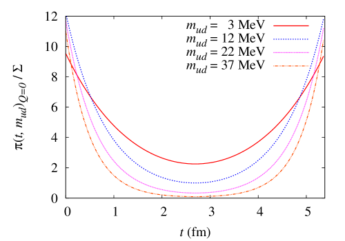
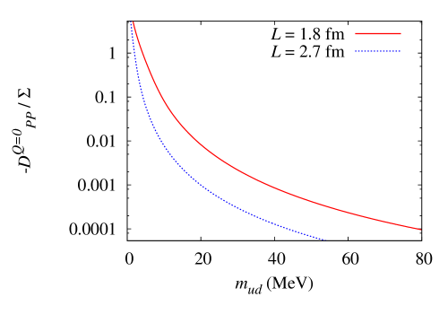
Figure 1: The $N_{f}=2+1$ ChPT prediction for the pion correlator $\mathcal{\pi}(t,m_{v})_{Q}$ (normalized by $\Sigma$) at $Q=0$ and $m_{v}=m_{ud}$. The finite periodic box size is $V=L^{3}T=(1.8~{}\mbox{fm})^{3}\times(5.4~{}\mbox{fm})$. We use $m_{s}=111$ MeV, $\Sigma^{\overline{\rm MS}}(2\;\mbox{GeV})=[234\;\mbox{MeV}]^{3}$, $F=71\;\mbox{MeV}$, $L_{4}^{r}(770\;\mbox{MeV})=0.0$, $L_{5}^{r}(770\;\mbox{MeV})=2.2\times 10^{-3}$, $L_{6}^{r}(770\;\mbox{MeV})=0.0$ and $L_{8}^{r}(770\;\mbox{MeV})=1.1\times 10^{-3}$ as the inputs.

Figure 2: The quark mass $m_{ud}(=m_{v})$ dependence of $-D^{Q}_{PP}$ (normalized by $\Sigma$) at $Q=0$. The same inputs as Fig. 2 are used.

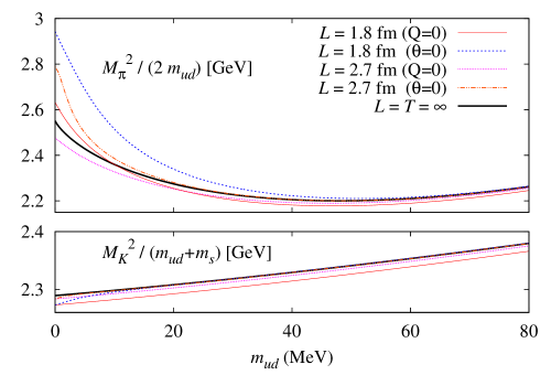
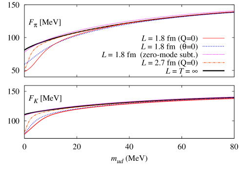
Figure 3: The up-down quark mass $m_{ud}(=m_{v})$ dependence of $(M_{vv}^{Q=0/\theta=0})^{2}/(2m_{ud})$ (upper panel) and $(M_{vs}^{Q=0/\theta=0})^{2}/(m_{ud}+m_{s})$ (lower) is plotted at different volume sizes. The same inputs as Fig. 2 are used.

Figure 4: $m_{ud}(=m_{v})$ dependence of the pion (upper panel) and kaon (lower) decay constants $F_{\pi}^{Q=0/\theta=0}$ and $F_{K}^{Q=0/\theta=0}$ at different volume sizes. The curves with the index “zero-mode subt.” denote $F_{\pi}^{\prime}$ or $F_{K}^{\prime}$. See the text for the notation. The same inputs as Fig. 2 are used.

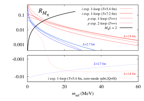
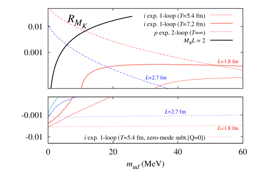
Figure 5: Comparison with the $p$ expansion results á la Lüscher formula Luscher:1985dn . Our new ChPT calculation ($i$ exp.) and the $p$ expansion ($p$ exp.) result from Ref. Colangelo:2005gd for $R_{M_{\pi}}$ (top) and $R_{M_{K}}$ (bottom) are drawn (note that one-loop correction in the $p$ expansion on $R_{M_{K}}$ is zero). The same inputs as Fig. 2 and those given in Ref. Colangelo:2005gd for the other higher LECs are used. The $M_{\pi}L=2$ (thick) curve is drawn using the two-loop result.

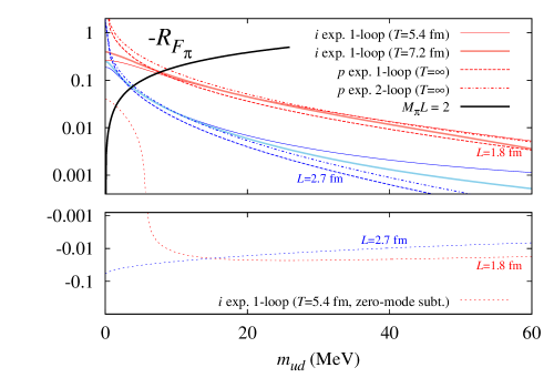
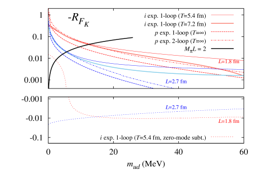
Figure 6: Comparison with the $p$ expansion results Colangelo:2005gd for $-R_{F_{\pi}}$ (top) and $-R_{F_{K}}$ (bottom).

VIII A short-cut prescription

We have performed a complete calculation to obtain the general form of the pseudoscalar correlation function in Eq. (93), which contains a conventional $\cosh$ function as well as a constant term and a contribution from 3-particle states.

It is no surprise that the constant term appears since the correlator in the conventional $p$ regime shows an unphysical infra-red divergence in the chiral limit. To remove this divergence, the zero-mode or the constant mode contribution is indispensable.

With this observation we find that the result in Eq. (93) is obtained by an easier prescription below. Starting from the conventional $p$ expansion formula in Eq. (103),

1. Replace the $Z$ factors with those from which the zero-mode contribution is subtracted, namely, $[Z^{ij}_{F}]_{p}$ and $[Z^{ij}_{M}]_{p}$ with $Z^{ij}_{F}$ and $Z^{ij}_{M}$.

2. Replace

   $$\frac{\cosh(M_{ij}^{\theta=0}(t-T/2))}{M_{ij}^{\theta=0}\sinh(M_{ij}^{\theta=0}T/2)}\;\;\;\mbox{with}\;\;\;\frac{\cosh(M_{ij}^{Q}(t-T/2))}{M_{ij}^{Q}\sinh(M_{ij}^{Q}T/2)}-\frac{2}{(M_{ij}^{Q})^{2}T}.$$ (187)

3. Multiply a factor coming from the exact zero-mode integrals, which can be read off from the coefficient of the $t$ dependent term or the $2Th_{1}(t/T)$ term in the $\epsilon$ expansion result. In the case of Eq. (93), it is $\frac{1}{2}\left(1+\mathcal{D}^{\rm eff}_{12}+\frac{Q^{2}}{\mu^{\rm eff}_{1}\mu^{\rm eff}_{2}}\right)$ obtained from Eq. (106). Note that the NLO condensate $\Sigma_{\rm eff}$, which contains chiral-log terms, should be used instead of the bare value $\Sigma$.

4. Add the constant and $r_{12}(t)$ terms if they exist in the $\epsilon$ expansion.

In fact, in a similar prescription, it is not difficult to obtain (a conjecture for) the axialvector-pseudoscalar and axialvector-axialvector correlators:

$$\mathcal{AP}(t,m_{1},m_{2})_{Q} \equiv \int d^{3}x\langle A_{0}(x)P(0)\rangle_{Q}$$ (188)

$$=\frac{\Sigma(Z_{F}^{12}Z_{M}^{12})^{2}}{2}\left[\left(1+\mathcal{D}^{\rm eff}_{12}+\frac{Q^{2}}{\mu^{\rm eff}_{1}\mu^{\rm eff}_{2}}\right)\left/\left(1+\frac{Q^{2}}{2\mu_{1}\mu_{2}}\right)\right.\right]\frac{\sinh(M_{12}^{Q}(t-T/2))}{\sinh(M_{12}^{Q}T/2)}$$

$$+\Sigma(Z_{F}^{12}Z_{M}^{12})^{2}\left[\left(\mathcal{S}^{\rm eff}_{1}+\mathcal{S}^{\rm eff}_{2}\right)-\left(1+\mathcal{D}^{\rm eff}_{12}+\frac{Q^{2}}{\mu^{\rm eff}_{1}\mu^{\rm eff}_{2}}\right)\left/\left(1+\frac{Q^{2}}{2\mu_{1}\mu_{2}}\right)\right.\right]\left(\frac{t}{T}-\frac{1}{2}\right)$$

$$-M_{12}^{2}\Sigma\frac{\mathcal{S}_{1}-\mathcal{S}_{2}}{\mu_{1}-\mu_{2}}\frac{\partial}{\partial t}(\partial_{M_{11}^{2}}r_{12}(t)+\partial_{M_{22}^{2}}r_{12}(t)),$$

$$\mathcal{AA}(t,m_{1},m_{2})_{Q} \equiv \int d^{3}x\langle A_{0}(x)A_{0}(0)\rangle_{Q}$$ (189)

$$= -\frac{\Sigma(Z_{F}^{12}Z_{M}^{12})^{2}}{2}(m_{1}+m_{2})\left(\mathcal{S}^{\rm eff}_{1}+\mathcal{S}^{\rm eff}_{2}\right)\frac{\cosh(M_{12}^{Q}(t-T/2))}{M_{12}^{Q}\sinh(M_{12}^{Q}T/2)}$$

$$+\frac{(FZ^{12}_{F})^{2}}{T}\left[\left(\mathcal{S}^{\rm eff}_{1}+\mathcal{S}^{\rm eff}_{2}\right)\left/\left(1+\frac{Q^{2}}{2\mu_{1}\mu_{2}}\right)\right.-\left(1+\mathcal{D}_{12}^{\rm eff}-\frac{Q^{2}}{\mu_{1}^{\rm eff}\mu_{2}^{\rm eff}}\right)\right]$$

$$+\frac{T}{2V}\left(1-\mathcal{D}_{12}^{\rm eff}+\frac{Q^{2}}{\mu_{1}^{\rm eff}\mu_{2}^{\rm eff}}\right)\sum_{i}^{N_{f}}(\bar{k}_{00}(M_{1i}^{2})+\bar{k}_{00}(M_{2i}^{2})),$$

where

$$\bar{k}_{00}(M^{2}) \equiv \sum_{{\bf q}=(p_{1},p_{2},p_{3})}\frac{-1}{4\sinh^{2}(\sqrt{|{\bf q}|^{2}+M^{2}}\;T/2)}+\frac{1}{M^{2}T^{2}},$$ (190)

which is UV finite (and of course IR finite as well) and can be thus numerically evaluated.

We confirm that Eqs. (188) and Eq. (189) indeed converge to those in the $p$ expansion Aoki:2009mx for the larger masses and those in the $\epsilon$ expansion Damgaard:2007ep ; Bernardoni:2008ei near the chiral limit. The above prescription thus achieves at least a smooth interpolation between the $\epsilon$ and $p$ regimes. Note that the $\epsilon$ regime result is not found in the literature for the $\mathcal{AP}(t,m_{1},m_{2})_{Q}$ correlator. We present in Appendix E our own calculation.

Furthermore, we find a more non-trivial evidence that supports our prescription: the axial Ward-Takahashi identities

$$\frac{\partial}{\partial t}\mathcal{AP}(t,m_{1},m_{2})_{Q} = (m_{1}+m_{2})\mathcal{PP}(t,m_{1},m_{2})_{Q}$$ (191)

$$=\frac{\Sigma(Z_{F}^{12}Z_{M}^{12})^{2}}{2}\left[\left(1+\mathcal{D}^{\rm eff}_{12}+\frac{Q^{2}}{\mu^{\rm eff}_{1}\mu^{\rm eff}_{2}}\right)\left/\left(1+\frac{Q^{2}}{2\mu_{1}\mu_{2}}\right)\right.\right]\frac{M_{12}^{Q}\cosh(M_{12}^{Q}(t-T/2))}{\sinh(M_{12}^{Q}T/2)}$$

$$+\left.\frac{\Sigma(Z_{F}^{12}Z_{M}^{12})^{2}}{T}\right[\left(\mathcal{S}^{\rm eff}_{1}+\mathcal{S}^{\rm eff}_{2}\right)-\left.\left(1+\mathcal{D}^{\rm eff}_{12}+\frac{Q^{2}}{\mu^{\rm eff}_{1}\mu^{\rm eff}_{2}}\right)\left/\left(1+\frac{Q^{2}}{2\mu_{1}\mu_{2}}\right)\right.\right]$$

$$-2\Sigma\frac{\mathcal{S}_{1}-\mathcal{S}_{2}}{\mu_{1}-\mu_{2}}M_{12}^{2}r_{12}(t)+{\cal O}(p^{4}),$$

and

$$-\frac{\partial}{\partial t}\mathcal{AA}(t,m_{1},m_{2})_{Q} = (m_{1}+m_{2})\mathcal{AP}(t,m_{1},m_{2})_{Q}$$

$$= \Sigma(Z_{F}^{12}Z_{M}^{12})^{2}(m_{1}+m_{2})\frac{\mathcal{S}^{\rm eff}_{1}+\mathcal{S}^{\rm eff}_{2}}{2}\frac{\sinh(M_{12}^{Q}(t-T/2))}{\sinh(M_{12}^{Q}T/2)}+{\cal O}(p^{4}),$$

are precisely satisfied. Here we have used

$$\left[\left(\mathcal{S}^{\rm eff}_{1}+\mathcal{S}^{\rm eff}_{2}\right)-\left(1+\mathcal{D}^{\rm eff}_{12}+\frac{Q^{2}}{\mu^{\rm eff}_{1}\mu^{\rm eff}_{2}}\right)\left/\left(1+\frac{Q^{2}}{2\mu_{1}\mu_{2}}\right)\right.\right]\left(\frac{t}{T}-\frac{1}{2}\right)$$ (193)

$$= \left[\left(\mathcal{S}^{\rm eff}_{1}+\mathcal{S}^{\rm eff}_{2}\right)-\left(1+\mathcal{D}^{\rm eff}_{12}+\frac{Q^{2}}{\mu^{\rm eff}_{1}\mu^{\rm eff}_{2}}\right)\left/\left(1+\frac{Q^{2}}{2\mu_{1}\mu_{2}}\right)\right.\right]\frac{\sinh(M_{12}^{Q}(t-T/2))}{2\sinh(M_{12}^{Q}T/2)},$$

which is valid up to a higher order contribution near the chiral limit, and

$$\frac{\partial^{2}}{\partial t^{2}}(\partial_{M_{ii}^{2}}r_{12}(t)) = r_{12}(t)+{\cal O}(M_{ii}^{2})\;\;\;\;\;(i=1,2).$$ (194)

Our results in Eqs.(93), (188) and (189) not only smoothly connect the $\epsilon$ and $p$ regimes but also keep the symmetry of the theory even in the intermediate region.

IX Conclusion

With the new perturbative scheme of ChPT proposed in Ref. Damgaard:2008zs , we have calculated the two-point correlation function in the pseudoscalar channel. The counting rule for the computation is essentially the same as in the conventional $p$ expansion (except for the additional rule for the mixing term of the zero and non-zero modes) while some of the zero-mode integrals are performed non-perturbatively as in the $\epsilon$ expansion.

As seen in Eqs.(93) and Eq.(124), the correlator is expressed by a hyperbolic cosine function of time $t$ plus an additional constant term as well as a non-trivial contribution from three-particle states, which smoothly interpolates the $p$ regime results and those in the $\epsilon$ regime.

The presence of the constant term in the correlator was known as a remarkable feature of the $\epsilon$ expansion. We have found that this constant plays an essential role in canceling the unphysical divergence coming from the $\cosh$ term in the $p$ expansion and keep the correlator always IR finite.

Giving examples for the $N_{f}=2$ and 2+1 theories, we have proposed a new method of determining the meson masses and decay constants from lattice QCD data obtained in a finite volume. Once one has a good control of the chiral condensate $\Sigma$, and therefore, of the non-trivial coefficients $C_{PP}^{Q}$, $D_{PP}^{Q}$ and $E_{PP}^{Q}$ in the correlators Eqs. (124) and (133), the zero-mode contributions can be subtracted and the remaining meson masses (see Fig. 4) and decay constants (Fig. 4) show a much milder volume dependence. Our results will be useful to precisely estimate the finite volume effects in lattice QCD data for the pion mass $M_{\pi}$ and kaon mass $M_{K}$, as well as their decay constants $F_{\pi}$ and $F_{K}$.

From our calculation we have found a short-cut prescription as shown in Section VIII. According to this greatly simplified scheme, we have derived the axialvector-pseudoscalar and axialvector-axialvector correlators. It turned out that these results not only give a smooth interpolation between the $\epsilon$ and $p$ regimes but also keep the axial Ward-Takahashi identities at an arbitrary choice of quark masses. It will be important to check if this simplified prescription is valid for the other quantities like three or four point functions.

Appendix A $\xi$ correlators in finite volume

Integrals over $\xi$ fields are expressed by $\bar{\Delta}(x,M^{2})$ and $\bar{G}(x,M_{1}^{2},M_{2}^{2})$ defined by Eqs. (11) and (12). Here we summarize useful formulas in the calculation of meson correlators.

We first note that even simple (three-dimensional) integrals and derivatives of them have unusual forms like

$$\int d^{3}x\;\bar{\Delta}(x,M^{2}) = \frac{\cosh(M(t-T/2))}{2M\sinh(MT/2)}-\frac{1}{M^{2}T},$$ (195)

$$\partial_{\mu}^{2}\bar{\Delta}(x,M^{2}) = M^{2}\bar{\Delta}(x,M^{2})+\frac{1}{V},$$ (196)

due to absence of the zero-mode.

For the ${\cal O}(S_{I}^{(1)})$ contribution, we need

$$\int d^{4}y\bar{\Delta}(x-y,M_{1}^{2})\bar{\Delta}(y,M_{2}^{2}) = \frac{1}{V}\sum_{p\neq 0}\frac{e^{ipx}}{(p^{2}+M_{1}^{2})(p^{2}+M_{2}^{2})}$$ (197)

$$= \frac{1}{M_{2}^{2}-M_{1}^{2}}\left(\bar{\Delta}(x,M_{1}^{2})-\bar{\Delta}(x,M_{2}^{2})\right).$$

which becomes $-\partial_{M^{2}}\bar{\Delta}(x,M^{2})|_{M^{2}=M_{1}^{2}}$ in the limit $M^{2}_{1}=M^{2}_{2}$.

In the same way,

$$\int d^{4}y\bar{\Delta}(x-y,M_{1}^{2})\bar{G}(y,M_{2}^{2},M_{3}^{2}) = \frac{1}{M_{2}^{2}-M_{1}^{2}}\left(\bar{G}(x,M_{1}^{2},M_{3}^{2})-\bar{G}(x,M_{2}^{2},M_{3}^{2})\right),$$ (198)

which can be expressed in two different ways:

$$= \frac{1}{M_{3}^{2}-M_{2}^{2}}\left(\bar{G}(x,M_{1}^{2},M_{2}^{2})-\bar{G}(x,M_{1}^{2},M_{3}^{2})\right),$$ (199)

$$= \frac{1}{M_{3}^{2}-M_{1}^{2}}\left(\bar{G}(x,M_{1}^{2},M_{2}^{2})-\bar{G}(x,M_{2}^{2},M_{3}^{2})\right).$$

For ${\cal O}((S_{I}^{(1)})^{2})$ contributions, we use

$$\int d^{4}y\,d^{4}z\,\bar{\Delta}(x-y,M_{1}^{2})\bar{\Delta}(y-z,M_{2}^{2})\bar{\Delta}(z,M_{1}^{2})=\frac{1}{V}\sum_{p\neq 0}\frac{e^{ipx}}{(p^{2}+M_{1}^{2})^{2}(p^{2}+M_{2}^{2})}$$

$$=\frac{1}{(M_{2}^{2}-M_{1}^{2})^{2}}\left(\bar{\Delta}(x,M_{2}^{2})-\bar{\Delta}(x,M_{1}^{2})\right)-\left.\frac{1}{M_{2}^{2}-M_{1}^{2}}\partial_{M^{2}}\bar{\Delta}(x,M^{2})\right|_{M^{2}=M_{1}^{2}},$$ (200)

whose degenerate limit, $M_{1}^{2}=M_{2}^{2}$, becomes $(\partial_{M^{2}})^{2}\bar{\Delta}(x,M^{2})|_{M^{2}=M_{1}^{2}}$. We also need

$$\int d^{4}y\,d^{4}z\,\bar{\Delta}(x-y,M_{1}^{2})\bar{G}(y-z,M_{2}^{2},M_{3}^{2})\bar{\Delta}(z,M_{1}^{2})\hskip 144.54pt$$

$$=\frac{\bar{G}(x,M_{1}^{2},M_{1}^{2})+\bar{G}(x,M_{2}^{2},M_{3}^{2})-\bar{G}(x,M_{1}^{2},M_{3}^{2})-\bar{G}(x,M_{1}^{2},M_{2}^{2})}{(M_{2}^{2}-M_{1}^{2})(M_{3}^{2}-M_{1}^{2})},$$ (201)

which becomes in the limit $M_{2}^{2}=M_{3}^{2}$,

$$=\frac{\bar{G}(x,M_{1}^{2},M_{1}^{2})+\bar{G}(x,M_{2}^{2},M_{2}^{2})-2\bar{G}(x,M_{1}^{2},M_{2}^{2})}{(M_{2}^{2}-M_{1}^{2})^{2}}.$$ (202)

For the disconnected part, we compute

$$\int d^{4}x\bar{\Delta}(x,M_{1}^{2})\bar{\Delta}(x,M_{2}^{2}) = \frac{1}{M_{2}^{2}-M_{1}^{2}}\left(\bar{\Delta}(0,M_{1}^{2})-\bar{\Delta}(0,M_{2}^{2})\right),$$ (203)

and

$$\int d^{4}x\bar{\Delta}(x,M_{1}^{2})\bar{G}(x,M_{2}^{2},M_{3}^{2}) = \frac{1}{2}\left[\frac{1}{M_{1}^{2}-M_{2}^{2}}\left(\bar{G}(0,M_{2}^{2},M_{3}^{2})-\bar{G}(0,M_{1}^{2},M_{3}^{2})\right)\right.$$ (204)

$$\left.+\frac{1}{M_{1}^{2}-M_{3}^{2}}\left(\bar{G}(0,M_{2}^{2},M_{3}^{2})-\bar{G}(0,M_{1}^{2},M_{2}^{2})\right)\right],$$

of which divergent part is treated with the dimensional regularization as usual.

Appendix B $\xi$ contraction in the pseudoscalar correlator

Here we summarize the $\xi$ contractions in $\langle P(x)P(0)\rangle^{00}$, $\langle P(x)P(0)\rangle^{10}$, $\langle P(x)P(0)\rangle^{20}$ and $\langle P(x)P(0)\rangle^{01}$.

The first leading contribution is given by

$$\langle P(x)P(0)\rangle^{00} = -\frac{\Sigma^{2}(Z_{M}^{12}Z_{F}^{12})^{4}}{4}\left\langle([U_{0}]_{12}-[U_{0}^{\dagger}]_{21})([U_{0}]_{21}-[U_{0}^{\dagger}]_{12})\right.$$ (205)

$$\left.\hskip 86.72377pt+\frac{1}{2}([U_{0}]_{12}-[U_{0}^{\dagger}]_{21})^{2}+\frac{1}{2}([U_{0}]_{21}-[U_{0}^{\dagger}]_{12})^{2}\right\rangle_{U_{0}}$$

$$-\frac{\Sigma^{2}}{8}\left(\Delta Z^{\Sigma}_{11}-\Delta Z^{\Sigma}_{22}\right)\langle([U_{0}]_{12}-[U_{0}^{\dagger}]_{21})^{2}-([U_{0}]_{21}-[U_{0}^{\dagger}]_{12})^{2}\rangle_{U_{0}}$$

$$+\frac{\Sigma^{2}}{2F^{2}}(Z_{F}^{12}(Z_{M}^{12})^{2})^{2}\bar{\Delta}(x,M_{12}^{\prime 2})\langle([U_{0}]_{11}+[U_{0}^{\dagger}]_{22})([U_{0}]_{22}+[U_{0}^{\dagger}]_{11})\rangle_{U_{0}}$$

$$+\frac{\Sigma^{2}}{2F^{2}}\sum_{j\neq 1}\bar{\Delta}(x,M_{j2}^{2})\langle[U_{0}]_{1j}[U_{0}^{\dagger}]_{j1}\rangle_{U_{0}}$$

$$+\frac{\Sigma^{2}}{2F^{2}}\sum_{i\neq 2}\bar{\Delta}(x,M_{i1}^{2})\langle[U_{0}]_{2i}[U_{0}^{\dagger}]_{i2}\rangle_{U_{0}}$$

$$-\frac{\Sigma^{2}}{2F^{2}}\bar{G}(x,M_{11}^{2},M_{22}^{2})\langle([U_{0}]_{12}+[U_{0}^{\dagger}]_{21})([U_{0}]_{21}+[U_{0}^{\dagger}]_{12})\rangle_{U_{0}}$$

$$+\frac{\Sigma^{2}}{4F^{2}}\bar{\Delta}(x,M_{22}^{2})\langle([U_{0}]_{12})^{2}+([U_{0}^{\dagger}]_{21})^{2}\rangle_{U_{0}}$$

$$+\frac{\Sigma^{2}}{4F^{2}}\bar{\Delta}(x,M_{11}^{2})\langle([U_{0}]_{21})^{2}+([U_{0}^{\dagger}]_{12})^{2}\rangle_{U_{0}}$$

$$-\frac{\Sigma^{2}}{4F^{2}}\bar{G}(x,M_{22}^{2},M_{22}^{2})\langle([U_{0}]_{12}+[U_{0}^{\dagger}]_{21})^{2}\rangle_{U_{0}}$$

$$-\frac{\Sigma^{2}}{4F^{2}}\bar{G}(x,M_{11}^{2},M_{11}^{2})\langle([U_{0}]_{21}+[U_{0}^{\dagger}]_{12})^{2}\rangle_{U_{0}},$$

where we have used

$$\Sigma_{\rm eff}^{2}\left(1-\Delta Z^{\Sigma}_{22}+\frac{16L_{8}}{F^{2}}M_{12}^{2}\right)\left(1-\Delta Z^{\Sigma}_{11}+\frac{16L_{8}}{F^{2}}M_{12}^{2}\right)=\Sigma^{2}(Z_{M}^{12}Z_{F}^{12})^{4}.$$

Next we calculate the ${\cal O}(\mathcal{S}_{I}^{(1)})$ contribution. In this NLO part, we can set $Z_{\xi}^{ij}=Z_{F}^{ij}=Z_{M}^{ij}=1$. Note that $\xi$ contractions have to be all connected since the self-contraction is not allowed in the NSC vertex in $\mathcal{S}_{I}^{(1)}$.

Using a notation given in Eq. (75) and the integration formulas given in Appendix A, we obtain

$$\langle P(x)P(0)\rangle^{10} = \frac{\Sigma^{2}}{2F^{2}}2\left\langle[\mathcal{R}]_{11}+[\mathcal{R}]_{22}\right\rangle_{U_{0}}\left.\left(\frac{\Sigma}{F^{2}}\partial_{M^{2}}\right)\bar{\Delta}(x,M^{2})\right|_{M^{2}=M_{12}^{2}}$$

$$-\frac{\Sigma^{2}}{2F^{2}}\sum^{N_{f}}_{j\neq 1}\frac{\langle[\mathcal{R}]_{j1}[U_{0}]_{1j}+[\mathcal{R}]_{1j}[U^{\dagger}_{0}]_{j1}\rangle_{U_{0}}}{m_{j}-m_{1}}\left(\bar{\Delta}(x,M_{12}^{2})-\bar{\Delta}(x,M_{2j}^{2})\right)$$

$$-\frac{\Sigma^{2}}{2F^{2}}\sum^{N_{f}}_{i\neq 2}\frac{\langle[\mathcal{R}]_{i2}[U_{0}]_{2i}+[\mathcal{R}]_{2i}[U^{\dagger}_{0}]_{i2}\rangle_{U_{0}}}{m_{i}-m_{2}}\left(\bar{\Delta}(x,M_{12}^{2})-\bar{\Delta}(x,M_{1i}^{2})\right)$$

$$-\frac{\Sigma^{2}}{2F^{2}}\frac{\langle[\mathcal{R}]_{12}[U^{\dagger}_{0}]_{12}+[U_{0}]_{21}[\mathcal{R}]_{21}\rangle_{U_{0}}}{m_{1}-m_{2}}\left(\bar{\Delta}(x,M_{12}^{2})-\bar{\Delta}(x,M_{11}^{2})\right)$$

$$-\frac{\Sigma^{2}}{2F^{2}}\frac{\langle[\mathcal{R}]_{21}[U^{\dagger}_{0}]_{21}+[U_{0}]_{12}[\mathcal{R}]_{12}\rangle_{U_{0}}}{m_{2}-m_{1}}\left(\bar{\Delta}(x,M_{12}^{2})-\bar{\Delta}(x,M_{22}^{2})\right)$$

$$+\frac{\Sigma^{2}}{2F^{2}}\frac{\langle[\mathcal{R}]_{12}([U_{0}]_{21}+[U_{0}^{\dagger}]_{12})+([U_{0}]_{21}+[U_{0}^{\dagger}]_{12})[\mathcal{R}]_{21}\rangle_{U_{0}}}{m_{1}-m_{2}}$$

$$\hskip 144.54pt\times\left(\bar{G}(x,M_{11}^{2},M_{22}^{2})-\bar{G}(x,M_{11}^{2},M_{11}^{2})\right)$$

$$+\frac{\Sigma^{2}}{2F^{2}}\frac{\langle[\mathcal{R}]_{21}([U_{0}]_{12}+[U_{0}^{\dagger}]_{21})+([U_{0}]_{12}+[U_{0}^{\dagger}]_{21})[\mathcal{R}]_{12}\rangle_{U_{0}}}{m_{2}-m_{1}}$$

$$\hskip 144.54pt\times\left(\bar{G}(x,M_{11}^{2},M_{22}^{2})-\bar{G}(x,M_{22}^{2},M_{22}^{2})\right).$$

For the ${\cal O}\left((\mathcal{S}_{I}^{(1)})^{2}\right)$ contribution we have both connected and disconnected parts. Note that we can set $Z_{\xi}^{ij}=Z_{F}^{ij}=Z_{M}^{ij}=1$ here, too.

The connected part (noted by the subscript “$con$”) is given by

$$\langle P(x)P(0)\rangle^{20}_{con} = \left.\frac{\Sigma^{2}}{2F^{2}}\right[$$ (207)

$$-\left(\sum_{j\neq 1}\frac{\langle[\mathcal{R}]_{1j}[\mathcal{R}]_{j1}\rangle_{U_{0}}}{(m_{j}-m_{1})}+\sum_{i\neq 2}\frac{\langle[\mathcal{R}]_{2i}[\mathcal{R}]_{i2}\rangle_{U_{0}}}{(m_{i}-m_{2})}\right)\left.\left(\frac{\Sigma}{F^{2}}\partial_{M^{2}}\right)\bar{\Delta}(x,M^{2})\right|_{M^{2}=M_{12}^{2}}$$

$$-\sum_{j\neq 1}\frac{\langle[\mathcal{R}]_{1j}[\mathcal{R}]_{j1}\rangle_{U_{0}}}{(m_{j}-m_{1})^{2}}\left(\bar{\Delta}(x,M_{12}^{2})-\bar{\Delta}(x,M_{2j}^{2})\right)$$

$$-\sum_{i\neq 2}\frac{\langle[\mathcal{R}]_{2i}[\mathcal{R}]_{i2}\rangle_{U_{0}}}{(m_{i}-m_{2})^{2}}\left(\bar{\Delta}(x,M_{12}^{2})-\bar{\Delta}(x,M_{1i}^{2})\right)$$

$$+\frac{\langle([\mathcal{R}]_{12})^{2}+([\mathcal{R}]_{21})^{2}\rangle_{U_{0}}}{2(m_{2}-m_{1})^{2}}\left(\bar{\Delta}(x,M_{11}^{2})+\bar{\Delta}(x,M_{22}^{2})-2\bar{\Delta}(x,M_{12}^{2})\right)$$

$$+\left.\frac{\langle 2[\mathcal{R}]_{12}[\mathcal{R}]_{21}+([\mathcal{R}]_{12})^{2}+([\mathcal{R}]_{21})^{2}\rangle_{U_{0}}}{(m_{1}-m_{2})^{2}}\bar{A}(x,M_{11}^{2},M_{22}^{2})\right].$$

For the disconnected contribution, we first calculate

$$\frac{1}{2}\langle(\mathcal{S}^{(1)}_{I})^{2}\rangle_{\xi} = -\frac{\Sigma^{2}V}{8F^{2}}\sum_{i\neq j}\frac{2\mathcal{R}_{ij}\mathcal{R}_{ji}}{M_{ii}^{2}-M_{jj}^{2}}\left(\Delta Z_{ii}^{\Sigma}-\Delta Z_{jj}^{\Sigma}\right),$$ (208)

using Eqs. (203) and (204) in Appendix A. Then we obtain (noted by the subscript “$dis$”)

$$\langle P(x)P(0)\rangle^{20}_{dis} = \frac{1}{2}\left[\langle\mathcal{\alpha}(U_{0})\langle(\mathcal{S}^{(1)}_{I})^{2}\rangle_{\xi}\rangle_{U_{0}}-\langle\mathcal{\alpha}(U_{0})\rangle_{U_{0}}\langle(\mathcal{S}^{(1)}_{I})^{2}\rangle_{\xi,U_{0}}\right]$$ (209)

$$+\frac{1}{2}\left[\langle\mathcal{\beta}(U_{0})\langle(\mathcal{S}^{(1)}_{I})^{2}\rangle_{\xi}\rangle_{U_{0}}-\langle\mathcal{\beta}(U_{0})\rangle_{U_{0}}\langle(\mathcal{S}^{(1)}_{I})^{2}\rangle_{\xi,U_{0}}\right]\bar{\Delta}(x,M_{12}^{2}),$$

where

$$\alpha(U_{0}) \equiv -\frac{\Sigma^{2}}{4}\left[([U_{0}]_{12}-[U_{0}^{\dagger}]_{21})([U_{0}]_{21}-[U_{0}^{\dagger}]_{12})\right.$$ (210)

$$\hskip 86.72377pt\left.+\frac{1}{2}([U_{0}]_{12}-[U_{0}^{\dagger}]_{21})^{2}+\frac{1}{2}([U_{0}]_{21}-[U_{0}^{\dagger}]_{12})^{2}\right],$$

$$\beta(U_{0}) \equiv \frac{\Sigma^{2}}{2F^{2}}([U_{0}]_{11}+[U_{0}^{\dagger}]_{22})([U_{0}]_{22}+[U_{0}^{\dagger}]_{11}).$$ (211)

Since $\Delta Z_{ii}^{\Sigma}$ rapidly decreases as the mass $m_{i}$ reaches the $\epsilon$ regime, the contribution is important only deeply inside the $p$ regime. Therefore, we can perturbatively perform this part of the $U_{0}$ integral in advance. Using the technique presented in Appendix D, the calculation is given by

$$\langle\mathcal{\alpha}(U_{0})\mathcal{R}_{ij}\mathcal{R}_{ji}\rangle_{U_{0}}-\langle\mathcal{\alpha}(U_{0})\rangle_{U_{0}}\langle\mathcal{R}_{ij}\mathcal{R}_{ji}\rangle_{U_{0}} = \frac{4\Sigma^{2}(m_{1}-m_{2})^{2}}{(\mu_{1}+\mu_{2})^{2}}(\delta_{i2}\delta_{j1}+\delta_{j2}\delta_{i1})+{\cal O}(p^{9}),$$ (212)

$$\langle\mathcal{\beta}(U_{0})\mathcal{R}_{ij}\mathcal{R}_{ji}\rangle_{U_{0}}-\langle\mathcal{\beta}(U_{0})\rangle_{U_{0}}\langle\mathcal{R}_{ij}\mathcal{R}_{ji}\rangle_{U_{0}} = {\cal O}(p^{10}),$$ (213)

where $\mu_{i}=m_{i}\Sigma V$ and we obtain

$$\langle P(x)P(0)\rangle^{20}_{dis} = -\frac{\Sigma^{2}(\mu_{1}-\mu_{2})}{(\mu_{1}+\mu_{2})^{2}}\left\langle\frac{[U_{0}+U_{0}^{\dagger}]_{11}}{2}+\frac{[U_{0}+U_{0}^{\dagger}]_{22}}{2}\right\rangle_{U_{0}}\left(\frac{1}{2}\Delta Z_{11}^{\Sigma}-\frac{1}{2}\Delta Z_{22}^{\Sigma}\right),$$

where we have used

$$2 = \left\langle\frac{[U_{0}+U_{0}^{\dagger}]_{11}}{2}+\frac{[U_{0}+U_{0}^{\dagger}]_{22}}{2}\right\rangle_{U_{0}}+{\cal O}(p^{2})$$ (215)

for the later convenience.

Finally let us calculate the ${\cal O}(\mathcal{S}_{I}^{(2)})$ contribution. As in the calculation above, using the technique in Appendix D, we obtain

$$\langle P(x)P(0)\rangle^{01} = -\frac{\Sigma^{2}}{(\mu_{1}+\mu_{2})^{2}}\left\langle\frac{[U_{0}+U_{0}^{\dagger}]_{11}}{2}+\frac{[U_{0}+U_{0}^{\dagger}]_{22}}{2}\right\rangle_{U_{0}}$$ (216)

$$\times\left[\mu_{1}\left(-\Delta Z_{11}^{\Sigma}+\frac{16L_{8}}{F^{2}}M_{12}^{2}\right)+\mu_{2}\left(-\Delta Z_{22}^{\Sigma}+\frac{16L_{8}}{F^{2}}M_{12}^{2}\right)\right].$$

Here we note

$$\langle P(x)P(0)\rangle^{20}_{dis}+\langle P(x)P(0)\rangle^{01}$$ (217)

$$= \frac{\Sigma^{2}}{(\mu_{1}+\mu_{2})}\left\langle\frac{[U_{0}+U_{0}^{\dagger}]_{11}}{2}+\frac{[U_{0}+U_{0}^{\dagger}]_{22}}{2}\right\rangle_{U_{0}}\left(\frac{\Sigma_{\rm eff}}{\Sigma}-(Z_{M}^{12}Z_{F}^{12})^{2}\right).$$

In order to obtain the final expression in Eq. (93), we use

$$-\frac{\Sigma^{2}}{4}(Z_{M}^{12}Z_{F}^{12})^{4}\mathcal{C}^{0a}+\frac{\Sigma^{2}}{\mu_{1}+\mu_{2}}\left(\frac{\Sigma_{\rm eff}}{\Sigma}-(Z_{M}^{12}Z_{F}^{12})^{2}\right)\mathcal{C}^{0b} = \Sigma^{2}(Z_{M}^{12}Z_{F}^{12})^{2}\frac{\mathcal{S}^{\rm eff}_{1}+\mathcal{S}^{\rm eff}_{2}}{\mu_{1}+\mu_{2}},$$ (218)

neglecting the higher order contributions.

Appendix C $U_{0}$ integrals

The zero-mode $U_{0}$ integrals of various matrix elements have been calculated in Ref. Damgaard:2007ep . Here we summarize the results in our notation for this paper.

$$\frac{1}{2}\left\langle[U_{0}]_{vv}-[U_{0}^{\dagger}]_{vv}\right\rangle_{U_{0}} = -\frac{Q}{\mu_{v}},$$ (219)

$$\frac{1}{4}\left\langle\left([U_{0}]_{vv}-[U_{0}^{\dagger}]_{vv}\right)^{2}\right\rangle_{U_{0}} = -\frac{\mathcal{S}_{v}}{\mu_{v}}+\frac{Q^{2}}{\mu_{v}^{2}},$$ (220)

$$\frac{1}{4}\left\langle\left([U_{0}]_{v_{1}v_{1}}-[U_{0}^{\dagger}]_{v_{1}v_{1}}\right)\left([U_{0}]_{v_{2}v_{2}}-[U_{0}^{\dagger}]_{v_{2}v_{2}}\right)\right\rangle_{U_{0}} = \frac{Q^{2}}{\mu_{v_{1}}\mu_{v_{2}}},$$ (221)

$$\frac{1}{4}\left\langle\left([U_{0}]_{v_{1}v_{2}}\pm[U_{0}^{\dagger}]_{v_{2}v_{1}}\right)^{2}\right\rangle_{U_{0}}=\frac{1}{4}\left\langle\left([U_{0}]_{v_{2}v_{1}}\pm[U_{0}^{\dagger}]_{v_{1}v_{2}}\right)^{2}\right\rangle_{U_{0}} = \frac{\pm 1}{\mu_{v_{1}}^{2}-\mu_{v_{2}}^{2}}\left(\mu_{v_{1}}\mathcal{S}_{v_{1}}-\mu_{v_{2}}\mathcal{S}_{v_{2}}\right),$$

$$\frac{1}{4}\left\langle\left([U_{0}]_{v_{1}v_{2}}\pm[U_{0}^{\dagger}]_{v_{2}v_{1}}\right)\left([U_{0}]_{v_{2}v_{1}}\pm[U_{0}^{\dagger}]_{v_{1}v_{2}}\right)\right\rangle_{U_{0}} = \frac{1}{\mu_{v_{1}}^{2}-\mu_{v_{2}}^{2}}\left(\mu_{v_{2}}\mathcal{S}_{v_{1}}-\mu_{v_{1}}\mathcal{S}_{v_{2}}\right).$$

Here it is useful to define

$$\delta_{i}\mathcal{S}_{j} \equiv \lim_{N_{f}+N\to N_{f}}\frac{\partial}{\partial\mu_{i}}\mathcal{S}_{j},$$ (224)

or more explicitly,

$$\delta_{i}\mathcal{S}_{j}=\left\{\begin{array}[]{ll}\displaystyle\lim_{\mu_{b_{1}}\to\mu_{i},\mu_{b_{2}}\to\mu_{j}}\frac{\partial}{\partial\mu_{i}}\frac{\partial}{\partial\mu_{j}}\ln\mathcal{Z}^{Q}_{2,2+N_{f}}(\mu_{b_{1}},\mu_{b_{2}},\mu_{i},\mu_{j},\{\mu_{sea}\})&\mbox{($i\neq j$)},\\ \displaystyle\lim_{\mu_{b}\to\mu_{i}}\frac{\partial^{2}}{\partial\mu_{i}^{2}}\ln\mathcal{Z}^{Q}_{1,1+N_{f}}(\mu_{b},\mu_{i},\{\mu_{sea}\})&\mbox{($i=j$)}.\end{array}\right.$$ (227)

Note that the partial quenching is performed after the differentiation. Then $\mathcal{D}$’s can be expressed as

$$\mathcal{D}_{i} = \delta_{i}\mathcal{S}_{i}+\mathcal{S}_{i}^{2},$$ (228)

$$\mathcal{D}_{ij} = \delta_{i}\mathcal{S}_{j}+\mathcal{S}_{i}\mathcal{S}_{j}=\delta_{j}\mathcal{S}_{i}+\mathcal{S}_{i}\mathcal{S}_{j}.$$ (229)

We note

$$m_{i}(\mathcal{S}_{i}-1) \sim {\cal O}(p^{4}),$$ (230)

$$m_{j}m_{i}\delta_{j}\mathcal{S}_{i} \sim {\cal O}(p^{8}),$$ (231)

which is useful to simplify our results.

We also note that $\mathcal{D}_{vv}$ (or $\mathcal{D}_{12}$ in the degenerate case $m_{1}=m_{2}=m_{v}$) can be written in a simpler form than the original definition. Introducing simplified notations for the zero-mode partition functions:

$$\mathcal{Z}_{0} = \mathcal{Z}_{0,N_{f}}^{Q}(\{\mu_{sea}\}),$$ (232)

$$\mathcal{Z}_{1}(\mu_{b}|\mu_{v}) = \mathcal{Z}_{1,1+N_{f}}^{Q}(\mu_{b},\mu_{v},\{\mu_{sea}\}),$$ (233)

$$\mathcal{Z}_{2}(\mu_{b1},\mu_{b2}|\mu_{v1},\mu_{v2}) = \mathcal{Z}_{2,2+N_{f}}^{Q}(\mu_{b1},\mu_{b2},\mu_{v1},\mu_{v2},\{\mu_{sea}\}),$$ (234)

and noting that these partition functions satisfy

$$\lim_{\mu_{b}\to\mu_{v}}\mathcal{Z}_{1}(\mu_{b}|\mu_{v}) = \mathcal{Z}_{0},$$ (235)

$$\lim_{\mu_{b2}\to\mu_{v2}}\mathcal{Z}_{2}(\mu_{b1},\mu_{b2}|\mu_{v1},\mu_{v2}) = \mathcal{Z}_{1}(\mu_{b1}|\mu_{v1}),$$ (236)

$$\lim_{\mu_{b2}\to\mu_{v1}}\mathcal{Z}_{2}(\mu_{b1},\mu_{b2}|\mu_{v1},\mu_{v2}) = \mathcal{Z}_{1}(\mu_{b1}|\mu_{v2}),$$ (237)

it is easy to show

$$\left.\left(\frac{\partial}{\partial\mu_{bi}}+\frac{\partial}{\partial\mu_{vi}}\right)\mathcal{Z}_{2}(\mu_{b1},\mu_{b2}|\mu_{v1},\mu_{v2})\right|_{\mu_{bi}=\mu_{vi}}=0$$ (238)

for any $i$. We then obtain

$$\mathcal{D}_{vv} = -\left.\frac{1}{\mathcal{Z}_{0}}\frac{\partial}{\partial\mu_{b}}\frac{\partial}{\partial\mu_{v}}\mathcal{Z}_{1}(\mu_{b}|\mu_{v})\right|_{\mu_{b}=\mu_{v}},$$ (239)

which is used to obtain expressions in Eqs. (154) and Eq. (178).

Appendix D $U_{0}$ integrals in the $p$ regime

In our calculation, we sometimes encounters a situation that the zero-mode integrals are needed only in the perturbative $p$ regime. It is not impossible to nonperturbatively perform the zero-mode integrals even in such cases, but it is more convenient to go back to the perturbative analysis to obtain the final results in a simple form.

Let us start with an expansion of the $U_{0}$ field:

$$U_{0} = \exp\left(i\frac{\sqrt{2}\xi_{0}}{F}\right)=1+\frac{i\sqrt{2}\xi_{0}}{F}-\frac{1}{F^{2}}\xi_{0}^{2}+\cdots,$$ (240)

and give a Feynman rule for $\xi_{0}$

$$\langle[\xi_{0}]_{ij}[\xi_{0}]_{kl}\rangle = \delta_{il}\delta_{jk}\frac{1}{M_{ij}^{2}V}.$$ (241)

Note that it reproduces the ordinary propagator in the $p$ expansion together with $\bar{\Delta}(x,M_{ij}^{2})$. It is here important to note that $\xi_{0}$ is an element not of $SU(N)$ but of $U(N)$ Lie algebra and there is no diagonal contribution like non-zero mode $\xi$ has. Then we can calculate the zero-mode integrals in the $p$ regime as

$$\langle[U_{0}]_{ij}[U_{0}]_{kl}\rangle_{U_{0}} = -\delta_{il}\delta_{jk}\frac{2}{\mu_{i}+\mu_{j}}+{\cal O}(p^{3}),$$ (242)

$$\langle[U_{0}]_{ij}[U^{\dagger}_{0}]_{kl}\rangle_{U_{0}} = +\delta_{il}\delta_{jk}\frac{2}{\mu_{i}+\mu_{j}}+{\cal O}(p^{3}),$$ (243)

$$\frac{\left\langle[U_{0}]_{ij}[U_{0}]_{ji}[U_{0}+U_{0}^{\dagger}]_{kk}\right\rangle_{U_{0}}}{2}-\frac{\left\langle[U_{0}]_{ij}[U_{0}]_{ji}\right\rangle_{U_{0}}\left\langle[U_{0}+U_{0}^{\dagger}]_{kk}\right\rangle_{U_{0}}}{2} = 2(\delta_{ik}+\delta_{jk})\left(\frac{1}{\mu_{i}+\mu_{j}}\right)^{2},$$

$$\frac{\left\langle[U_{0}]_{ij}[U_{0}^{\dagger}]_{ji}[U_{0}+U_{0}^{\dagger}]_{kk}\right\rangle_{U_{0}}}{2}-\frac{\left\langle[U_{0}]_{ij}[U_{0}^{\dagger}]_{ji}\right\rangle_{U_{0}}\left\langle[U_{0}+U_{0}^{\dagger}]_{kk}\right\rangle_{U_{0}}}{2} = -2(\delta_{ik}+\delta_{jk})\left(\frac{1}{\mu_{i}+\mu_{j}}\right)^{2}.$$

These results can be, of course, confirmed by directly performing the exact group integrals and then taking the asymptotic expansion in large $m_{i}\Sigma V$’s.

Appendix E Axialvector-Pseudoscalar correlator in the pure $\epsilon$ regime

In this appendix we present the axialvector-pseudoscalar correlator in the $\epsilon$ regime, which is, to our knowledge, not found in the literature.

Since $M^{2}\sim{\cal O}(\epsilon^{4})$ is deep inside the $\epsilon$ regime, we can neglect the meson mass in the $Z$ factors: let us remove the superscripts and use notations such as $Z_{M}$, $Z_{F}$. We also note $\Sigma_{\rm eff}=\Sigma Z_{M}^{2}Z_{F}^{2}$ and $\Delta Z_{22}^{\Sigma}=0$ to NLO in the $\epsilon$ regime.

The source terms are then simplified as

$$P^{12}(x) = i\frac{\Sigma_{\rm eff}}{2}\left([U_{0}]_{12}-[U_{0}^{\dagger}]_{21}\right)$$ (246)

$$-\frac{\Sigma}{\sqrt{2}F}\sum_{i,j}\xi_{ij}(x)\left([U_{0}]_{1i}\delta_{j2}+\delta_{1i}[U_{0}^{\dagger}]_{j2}\right)Z_{\xi}Z_{F}(Z_{M})^{2}$$

$$-i\frac{\Sigma}{2F^{2}}\sum_{i,j}[\xi^{2}(x)]_{ij}^{NSC}\left([U_{0}]_{1i}\delta_{j2}-\delta_{1i}[U_{0}^{\dagger}]_{j2}\right),$$

$$P^{21}(x) = (1\leftrightarrow 2),$$ (247)

and the axialvector sources can be similarly written as

$$A_{0}^{12}(x) = -\frac{F}{\sqrt{2}}\sum_{i,j}[\partial_{0}\xi(x)]_{ji}\left([U^{\dagger}_{0}]_{i2}[U_{0}]_{1j}+\delta_{i2}\delta_{1j}\right)Z_{\xi}Z_{F}$$ (248)

$$+\frac{i}{2}\sum_{i,j}[\partial_{0}\xi\xi-\xi\partial_{0}\xi]^{NSC}_{ji}(x)\left([U_{0}^{\dagger}]_{i2}[U_{0}]_{1j}-\delta_{i2}\delta_{1j}\right),$$

$$A_{0}^{21}(x) = (1\leftrightarrow 2).$$ (249)

Note that the mass term is now an NLO contribution, which can be treated as a perturbative interaction term and one can omit the mass in the Feynman rule for $\xi$:

$$\langle\xi_{ij}(x)\xi_{kl}(y)\rangle_{\xi} = \delta_{il}\delta_{jk}\bar{\Delta}(x-y,0)-\delta_{ij}\delta_{kl}\bar{G}(x-y,0,0),$$ (250)

We therefore replace $\mathcal{S}_{I}^{(1)}$ by

$$\mathcal{S}_{I} \equiv \frac{\Sigma}{2F^{2}}\int d^{4}x{\rm Tr}\left[\mathcal{R}^{\prime}[\xi^{2}(x)]^{NSC}\right],$$ (251)

where

$$\mathcal{R}^{\prime} \equiv \mathcal{M}^{\dagger}U_{0}+U_{0}^{\dagger}\mathcal{M}+\frac{N_{f}}{\Sigma V}{\bf 1}.$$ (252)

Since $\mathcal{S}_{I}\sim{\cal O}(\epsilon^{2})$, it is sufficient to calculate

$$\langle A_{0}(x)P(0)\rangle = \frac{1}{2}\left[\langle A^{12}_{0}(x)P^{21}(0)+A^{12}_{0}(x)P^{12}(0)\rangle^{00}+\langle A^{12}_{0}(x)P^{21}(0)+A^{12}_{0}(x)P^{12}(0)\rangle^{10}\right]$$ (253)

$$+(1\leftrightarrow 2).$$

Noting $\left\langle[\partial_{0}\xi\xi-\xi\partial_{0}\xi]^{NSC}_{ji}(x)[\xi^{2}]^{NSC}_{kl}(0)\right\rangle_{\xi}=0$, and (see Ref. Bernardoni:2008ei )

$$\langle[U_{0}\mathcal{M}U_{0}]_{11}\rangle_{U_{0}} = m_{1}-\frac{2}{\Sigma V}(N_{f}+Q)\langle[U_{0}]_{11}\rangle_{U_{0}},$$ (254)

$$\langle[U^{\dagger}_{0}\mathcal{M}U^{\dagger}_{0}]_{11}\rangle_{U_{0}} = m_{1}-\frac{2}{\Sigma V}(N_{f}-Q)\langle[U^{\dagger}_{0}]_{11}\rangle_{U_{0}},$$ (255)

$$\left\langle\left([U_{0}]_{12}+[U_{0}^{\dagger}]_{12}\right)\left([U_{0}]_{21}+[U_{0}^{\dagger}]_{21}\right)\right\rangle_{U_{0}}$$

$$=\frac{1}{4}\left\langle 2\left([U_{0}]_{12}+[U_{0}^{\dagger}]_{21}\right)\left([U_{0}]_{21}+[U_{0}^{\dagger}]_{12}\right)+2\left([U_{0}]_{12}-[U_{0}^{\dagger}]_{21}\right)\left([U_{0}]_{21}-[U_{0}^{\dagger}]_{12}\right)\right.$$

$$\left.+\left([U_{0}]_{12}+[U_{0}^{\dagger}]_{21}\right)^{2}+\left([U_{0}]_{21}+[U_{0}^{\dagger}]_{12}\right)^{2}-\left([U_{0}]_{12}-[U_{0}^{\dagger}]_{21}\right)^{2}-\left([U_{0}]_{21}-[U_{0}^{\dagger}]_{12}\right)^{2}\right\rangle,$$

and using the integration formulas in Appendix A, we obtain the correlator,

$$\langle A_{0}(x)P(0)\rangle = \Sigma_{\rm eff}\left(1+\mathcal{D}_{12}^{\rm eff}+\frac{Q^{2}}{\mu^{\rm eff}_{1}\mu^{\rm eff}_{2}}\right)\partial_{0}\bar{\Delta}(x,M_{12}^{2})$$ (257)

$$+\Sigma_{\rm eff}\left[\mathcal{S}_{1}^{\rm eff}+\mathcal{S}_{2}^{\rm eff}-\left(1+\mathcal{D}_{12}^{\rm eff}+\frac{Q^{2}}{\mu^{\rm eff}_{1}\mu^{\rm eff}_{2}}\right)\right]\partial_{0}\bar{\Delta}(x,0)$$

$$-\left.M_{12}^{2}\Sigma\frac{\mathcal{S}_{1}-\mathcal{S}_{2}}{\mu_{1}-\mu_{2}}\partial_{M^{2}}\partial_{0}(\bar{G}(x,M^{2},0)+\bar{G}(x,0,M^{2}))\right|_{M=0}.$$

References

(1)
Y. Nambu and G. Jona-Lasinio,
Phys. Rev. 122, 345 (1961).
(2)
S. Weinberg,
Phys. Rev. 166, 1568 (1968).
(3)
J. Gasser and H. Leutwyler,
Annals Phys. 158, 142 (1984);
Nucl. Phys. B 250, 465 (1985).
(4)
J. Gasser and H. Leutwyler,
Phys. Lett. B 184, 83 (1987).
(5)
J. Gasser and H. Leutwyler,
Nucl. Phys. B 307, 763 (1988).
(6)
C. Bernard [MILC Collaboration],
Phys. Rev. D 65, 054031 (2002)
[arXiv:hep-lat/0111051].
(7)
G. Colangelo, S. Durr and C. Haefeli,
Nucl. Phys. B 721, 136 (2005)
[arXiv:hep-lat/0503014].
(8)
J. Gasser and H. Leutwyler,
Phys. Lett. B 188, 477 (1987).
(9)
H. Neuberger,
Phys. Rev. Lett. 60 (1988) 889.
(10)
F. C. Hansen,
Nucl. Phys. B 345, 685 (1990);
F. C. Hansen and H. Leutwyler,
Nucl. Phys. B 350, 201 (1991).
(11)
P. Hasenfratz and H. Leutwyler,
Nucl. Phys. B 343, 241 (1990).
(12)
H. Leutwyler and A. Smilga,
Phys. Rev. D 46, 5607 (1992).
(13)
P. H. Damgaard, M. C. Diamantini, P. Hernandez and K. Jansen,
Nucl. Phys. B 629 (2002) 445
[arXiv:hep-lat/0112016].
(14)
P. H. Damgaard, P. Hernandez, K. Jansen, M. Laine and L. Lellouch,
Nucl. Phys. B 656, 226 (2003)
[arXiv:hep-lat/0211020].
(15)
P. Hernandez and M. Laine,
JHEP 0301, 063 (2003)
[arXiv:hep-lat/0212014].
(16)
P. H. Damgaard and H. Fukaya,
Nucl. Phys. B 793, 160 (2008)
[arXiv:0707.3740 [hep-lat]].
(17)
F. Bernardoni and P. Hernandez,
JHEP 0710, 033 (2007)
[arXiv:0707.3887 [hep-lat]].
(18)
F. Bernardoni, P. H. Damgaard, H. Fukaya and P. Hernandez,
JHEP 0810, 008 (2008)
[arXiv:0808.1986 [hep-lat]].
(19)
G. Akemann, F. Basile and L. Lellouch,
JHEP 0812, 069 (2008)
[arXiv:0804.3809 [hep-lat]].
(20)
A. Shindler,
Phys. Lett. B 672, 82 (2009)
[arXiv:0812.2251 [hep-lat]].
(21)
O. Bar, S. Necco and S. Schaefer,
JHEP 0903, 006 (2009)
[arXiv:0812.2403 [hep-lat]].
(22)
F. Bernardoni, P. Hernandez and S. Necco,
JHEP 1001, 070 (2010)
[arXiv:0910.2537 [hep-lat]].
(23)
O. Bar, S. Necco and A. Shindler,
JHEP 1004, 053 (2010)
[arXiv:1002.1582 [hep-lat]].
(24)
F. Bernardoni, N. Garron, P. Hernandez, S. Necco and C. Pena,
arXiv:1008.1870 [hep-lat].
(25)
C. Lehner, S. Hashimoto and T. Wettig,
JHEP 1006, 028 (2010)
[arXiv:1004.5584 [hep-lat]].
(26)
T. DeGrand, Z. Liu and S. Schaefer,
Phys. Rev. D 74, 094504 (2006)
[Erratum-ibid. D 74, 099904 (2006)]
[arXiv:hep-lat/0608019].
(27)
C. B. Lang, P. Majumdar and W. Ortner,
Phys. Lett. B 649, 225 (2007)
[arXiv:hep-lat/0611010].
(28)
P. Hasenfratz, D. Hierl, V. Maillart, F. Niedermayer, A. Schafer, C. Weiermann and M. Weingart,
JHEP 0911, 100 (2009)
[arXiv:0707.0071 [hep-lat]].
(29)
H. Fukaya et al. [JLQCD collaboration],
Phys. Rev. D 77, 074503 (2008)
[arXiv:0711.4965 [hep-lat]].
(30)
A. Hasenfratz, R. Hoffmann and S. Schaefer,
Phys. Rev. D 78, 014515 (2008)
[arXiv:0805.2369 [hep-lat]].
(31)
A. Hasenfratz, R. Hoffmann and S. Schaefer,
Phys. Rev. D 78, 054511 (2008)
[arXiv:0806.4586 [hep-lat]].
(32)
O. Bar, S. Necco and S. Schaefer,
PoS LAT2009, 078 (2009)
[arXiv:0910.2372 [hep-lat]].
(33)
K. Jansen and A. Shindler,
PoS LAT2009, 070 (2009)
[arXiv:0911.1931 [hep-lat]].
(34)
P. H. Damgaard and H. Fukaya,
JHEP 0901, 052 (2009)
[arXiv:0812.2797 [hep-lat]].
(35)
P. H. Damgaard and S. M. Nishigaki,
Nucl. Phys. B 518, 495 (1998)
[arXiv:hep-th/9711023].
(36)
T. Wilke, T. Guhr and T. Wettig,
Phys. Rev. D 57, 6486 (1998)
[arXiv:hep-th/9711057].
(37)
G. Akemann and P. H. Damgaard,
Nucl. Phys. B 528, 411 (1998)
[arXiv:hep-th/9801133].
(38)
A. V. Smilga and J. Stern,
Phys. Lett. B 318, 531 (1993).
(39)
J. C. Osborn, D. Toublan and J. J. M. Verbaarschot,
Nucl. Phys. B 540, 317 (1999)
[arXiv:hep-th/9806110].
(40)
H. Fukaya, S. Aoki, S. Hashimoto, T. Kaneko, J. Noaki, T. Onogi and N. Yamada
[JLQCD collaboration],
Phys. Rev. Lett. 104, 122002 (2010)
[Erratum-ibid. 105, 159901 (2010)]
[arXiv:0911.5555 [hep-lat]].
(41)
H. Fukaya et al. [JLQCD and TWQCD collaborations],
arXiv:1012.4052 [hep-lat].
(42)
P. H. Damgaard and K. Splittorff,
Nucl. Phys. B 572, 478 (2000)
[arXiv:hep-th/9912146].
(43)
P. H. Damgaard and K. Splittorff,
Phys. Rev. D 62, 054509 (2000)
[arXiv:hep-lat/0003017].
(44)
P. H. Damgaard,
Phys. Lett. B 476, 465 (2000)
[arXiv:hep-lat/0001002].
(45)
J. Wess and B. Zumino,
Phys. Lett. B 37, 95 (1971).
(46)
E. Witten,
Nucl. Phys. B 223, 422 (1983).
(47)
K. Splittorff and J. J. M. Verbaarschot,
Phys. Rev. Lett. 90, 041601 (2003)
[arXiv:cond-mat/0209594].
(48)
Y. V. Fyodorov and G. Akemann,
JETP Lett. 77, 438 (2003)
[Pisma Zh. Eksp. Teor. Fiz. 77, 513 (2003)]
[arXiv:cond-mat/0210647].
(49)
K. Splittorff and J. J. M. Verbaarschot,
Nucl. Phys. B 683, 467 (2004)
[arXiv:hep-th/0310271].
(50)
J. Lenaghan and T. Wilke,
Nucl. Phys. B 624, 253 (2002)
[arXiv:hep-th/0108166].
(51)
S. Aoki and H. Fukaya,
Phys. Rev. D 81, 034022 (2010)
[arXiv:0906.4852 [hep-lat]].
(52)
Y. Y. Mao and T. W. Chiu [TWQCD Collaboration],
Phys. Rev. D 80, 034502 (2009)
[arXiv:0903.2146 [hep-lat]].
(53)
S. R. Sharpe and N. Shoresh,
Phys. Rev. D 62, 094503 (2000)
[arXiv:hep-lat/0006017].
(54)
J. Bijnens, N. Danielsson and T. A. Lahde,
Phys. Rev. D 73, 074509 (2006)
[arXiv:hep-lat/0602003].
(55)
M. Luscher,
Commun. Math. Phys. 104, 177 (1986).
(56)
H. Leutwyler,
Phys. Lett. B 189, 197 (1987).
(57) P. Hasenfratz and F. Niedermayer,
Z. Phys. B 92 (1993) 91 [arXiv:hep-lat/9212022].
(58)
P. Hasenfratz,
Nucl. Phys. B 828, 201 (2010)
[arXiv:0909.3419 [hep-th]].
(59)
W. Bietenholz et al.,
Phys. Lett. B 687, 410 (2010)
[arXiv:1002.1696 [hep-lat]].
(60)
M. Weingart,
arXiv:1006.5076 [hep-lat].
(61)
F. Niedermayer and C. Weiermann,
Nucl. Phys. B 842, 248 (2011)
[arXiv:1006.5855 [hep-lat]].
(62)
W. Bietenholz et al. [QCDSF Collaboration],
J. Phys. Conf. Ser. 287, 012016 (2011)
[arXiv:1103.3311 [hep-lat]].