Local classification of singular hexagonal 3-webs
with holomorphic Chern connection and infinitesimal symmetries

Abstract

We provide a complete classification of hexagonal singular 3-web germs in the complex plane, satisfying the following two conditions:

1) the Chern connection remains holomorphic at the singular point,

2) the web admits at least one infinitesimal symmetry at this point.
As a by-product, a classification of hexagonal weighted homogeneous 3-webs is obtained.

Key words: hexagonal 3-web, implicit ODE, Chern connection, infinitesimal symmetries.

AMS Subject classification: 53A60 (primary), 32S65 (secondary).

1 Introduction

A finite number of pairwise different foliations in the plane form a planar web. A point $q_{0}$ is called regular if for each pair of foliations the tangent lines to the leaves at this point are transverse to each other. The corresponding local object is called a non-singular web germ at $q_{0}$. Consider the group of diffeomorphism (or biholomorphism) germs and the corresponding equivalence relation. Clearly, each non-singular 2-web germ is equivalent to the 2-web germ formed by coordinate lines. The situation becomes more complicated for 3-webs. Blaschke discovered that generically even a regular 3-web germ is not equivalent to the web germ of three families of parallel lines [8]. From the differential-geometric point of view a nontrivial 3-web has a non-vanishing curvature 2-form.

Moreover, the invariant in question is topological in nature. Choose an arbitrary regular point $p_{0}$ in the plane, draw the leaves $L_{1},L_{2},L_{3}$ of the web through this point, take a point $p_{1}$ on $L_{1}$ and go around $p_{0}$ along the web leaves starting from $p_{1}$ and swapping the foliation each time when meeting $L_{1}$, $L_{2}$ or $L_{3}$. For the web equivalent to 3 families of parallel lines, which has zero curvature, one comes back to $p_{1}$. Less trivial is that the inverse is also true and the following 3 conditions are equivalent:

1. for each choice of $p_{0},p_{1}$, the constructed hexagon-like figure is closed,

2. the web is equivalent to 3 families of parallel lines,

3. the web curvature is zero.

(see [8, 9] and picture 1).

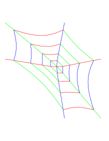
Figure 1: Briançon’s hexagons

The webs possessing any of the above properties are called hexagonal or flat. A sufficiently general class of 3-web germs can be described by binary forms:

$$K_{3}(x,y)dy^{3}+K_{2}(x,y)dy^{2}dx+K_{1}(x,y)dydx^{2}+K_{0}(x,y)dx^{3}=0,$$ (1)

where at least one of the germs $K_{i}$ does not vanish at $(0,0)$. Dividing the above form by $dx^{3}$ and by a non-vanishing coefficient one gets an implicit ODE, cubic in $p=\frac{dy}{dx}$. Rotating the coordinate axes, if necessary, one can reduce this equation to a monic one:

$$p^{3}+a(x,y)p^{2}+b(x,y)p+c(x,y)=0.$$ (2)

Its solutions form a hexagonal 3-web iff the coefficients of this cubic ODE satisfy a certain nonlinear partial differential equation (see Section 2). In this paper we study the complex analytic case, i.e., $K_{i}$ are germs of holomorphic function at $(\mathbb{C}^{2},0)$ and the equivalence relation is induced by the group of germs of biholomorphisms ${\rm Diff(\mathbb{C}^{2},0)}$.

Example 1

The classical Graf and Sauer theorem [19] claims that a 3-web of straight lines is hexagonal iff the web lines are tangents to an algebraic curve of class 3, i.e., the dual curve is cubic. This implies immediately that the following cubic Clairaut equation has a hexagonal 3-web of solutions:

$$p^{3}+px-y=0.$$

Its solutions are the lines $p=const$ enveloping a semicubic parabola (Fig. 2).

Example 2

Consider an associativity equation

$$u_{xxx}=u^{2}_{xyy}-u_{xxy}u_{yyy},$$ (3)

describing 3-dimensional Frobenius manifolds (see [12]). Each of its solutions $u(x,y)$ defines a characteristic web in the plane. This web is hexagonal; it follows from the results obtained in [26]. (See also [6], where a broader class of PDEs with flat characteristic 3-webs was studied.) Characteristics are integral curves of the vector field

$$\partial_{x}-\lambda(x,y)\partial_{y},$$

where $\lambda$ satisfy the characteristic equation

$$\lambda^{3}+u_{yyy}\lambda^{2}-2u_{xyy}\lambda+u_{xxy}=0.$$

For the solution $u=\frac{x^{2}y^{2}}{4}+\frac{x^{5}}{60}$, the characteristic equation becomes

$$p^{3}+2xp+y=0$$

after the substitution $x\to-x$, $y\to-y$, $\lambda\to-p$. The corresponding 3-web is shown in Fig. 2.

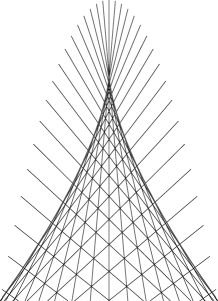
Figure 2: Solutions of $p^{3}+px-y=0$ and $p^{3}+2xp+y=0$ with horizontal y-axis.

Notice that the above web germs are not equivalent. We call a web germ at $q_{0}\in\mathbb{C}^{2}$ singular if at least two web directions coincide at $q_{0}$. The examples show that singular hexagonal web germs are not necessarily equivalent.

Curvature 2-form of a 3-web is defined as the external derivative $d(\gamma)$ of the Chern connection 1-form $\gamma$ (see [9] and Section 2). Thus, for hexagonal 3-webs, this form is closed. But it is not exact in general: on the discriminant curve of the web, where at least 2 foliations of the web are not transverse, the Chern connection form usually has a pole. For instance, for the first of the above examples we have

$$\gamma=\frac{6x^{2}dx+27ydy}{4x^{3}+27y^{2}},$$

whereas in the second example $\gamma$ is the zero 1-form, i.e. holomorphic. We are particularly interested in classification of singular webs whose Chern connection form remains holomorphic on the discriminant curve.

Observe that the above two 3-webs are invariant under the flow of the vector field $X=2x\partial_{x}+3y\partial_{y}.$ We say that web has an infinitesimal symmetry

$$X=\xi(x,y)\partial_{x}+\eta(x,y)\partial_{y},$$

if the local flow of the vector field $X$ maps the web leaves to the web leaves. Infinitesimal symmetries form a Lie algebra with respect to the Lie bracket. Cartan proved (see [10]) that at a regular point a 3-web either does not have infinitesimal symmetries (generic case), or has one-dimensional symmetry algebra (then in suitable coordinates it can be defined by the form $dx\cdot dy\cdot(dy+u(x+y)dx)=0$ with the symmetry $\partial_{y}-\partial_{x}$), or has a three-dimensional symmetry algebra (then it is equivalent to the web defined by the form $dx\cdot dy\cdot(dy+dx)=0$ with the symmetry algebra generated by $\{\partial_{x},\ \partial_{y},x\partial_{x}+y\partial_{y}\}$). In the last case, when the symmetry algebra has the largest possible dimension 3, the 3-web is hexagonal. Note that not all symmetries survive at a singular point; in the above examples the dimension of the symmetry algebra drops to 2 at a generic point of the discriminant curve and to 1 at the cusp point. The condition to have at least one-dimensional symmetry at a singular point is not trivial. The following equation has a flat 3-web of solutions but does not admit non-trivial symmetries at $(0,0)$

$$p^{3}-2x^{2}y(1+x^{2})p+8x^{3}y^{2}=0.$$

The objective of this paper is to describe singular hexagonal 3-web germs such that:

1. the Chern connection form is holomorphic,

2. the web has at least one infinitesimal symmetry.

The principal motivation for this problem comes from the geometric theory of Frobenius manifolds. Namely characteristics on solutions of WDVV associativity equation (see Example 2) form a hexagonal 3-web, as was observed by Ferapontov. In fact, for this web, the Chern connection is holomorphic, i.e locally exact. Moreover, the associativity condition in suitable flat coordinates assumes two essentially different forms: either as equation (3) or as the following one (see [12]):

$$u_{xxx}u_{yyy}-u_{xxy}u_{xyy}=1.$$ (4)

Now the characteristic 3-webs are defined by the following ODE:

$$u_{yyy}p^{3}+u_{xyy}p^{2}-u_{xxy}p-u_{xxx}=0.$$

We observe that the Chern connection is zero on the characteristic 3-web of each solution $u(x,y)$ of equation (3) and is holomorphic on the characteristic 3-web of each solution of (4). See [4] and [5] for more detail and a geometrical interpretation of this fact. Moreover, the characteristic 3-web for a Frobenius 3-web germ can be constructed in a pure geometrical way sturting from a Frobenius 3-fold, as was shown in [4].

Further, if a solution of the associativity equation corresponds to some geometric Frobenius structure, as defined by Dubrovin in [12], the characteristic 3-web has an infinitesimal symmetry, inherited from the so-called Euler vector field (see [4])

$$E=w_{x}x\frac{\partial}{\partial x}+w_{y}y\frac{\partial}{\partial y},\ \ \ \ \ \ w_{x},w_{y}={\rm const}.$$ (5)

Equations and webs symmetric with respect to such dilatation symmetry are called weighted homogeneous. In what follows we call the operator of type (5) Euler vector field.

Hexagonal 3-webs, satisfying the above two conditions, have nice properties from the purely mathematical point of view. Recall that a 3-web is hexagonal iff its foliations have first integrals $u_{i}$ satisfying $u_{1}+u_{2}+u_{3}=0$. Then the finiteness of the Chern connection form implies that these integrals are integer algebraic over the ring of holomorphic function germs. The corresponding algebraic equation for $u_{i}$ at a singular point $q_{0}$ can be read off the infinitesimal symmetry, provided that this symmetry has an equilibrium point at $q_{0}$. Further, if the monodromy group, permuting the web leaves on going around the discriminant curve, is ”maximal possible”, i.e. $S_{3}$ for the triple root of equation (1) or $Z_{2}$ for a double root, we prove also the existence of infinitesimal symmetries. Namely we prove that if the Chern connection form is exact and defined at some neighborhood of a singular point $q_{0}$, then there is at least 2-dimensional symmetry algebra at $q_{0}$ for a double root and at least 1-dimensional symmetry algebra for a triple root. (See section 3.)

The main result of the paper is a complete classification of the 3-web germs of the class introduced above. The list consists of 5 equations and 3 infinite series (see Theorems 9 and 10). It is remarkable that the normal forms can be written in terms of polynomials, the function $\tan$ and Legendre‘s functions $P^{\mu}_{\nu},Q^{\mu}_{\nu}$. The key observation that allowed the obtained classification is that each symmetry operator vanishing at the singular point is equivalent to dilataion symmetry (see Theorem 2). Thus, as a by-product, we obtained a complete classification of weighted homogeneous hexagonal 3-webs, i.e. having an infinitesimal symmetry of the form (5) (and possibly singular Chern connection). We also provide invariants distinguishing the normal forms for these two classifications.

Symmetries, vanishing at singular points, comes quite natural by singular webs. For instance, it is immediate that if equation (2) admits a non-trivial symmetry at a singular point of the discriminant curve, this point is necessary a singular point of the vector field $X$.

In the literature mainly symmetries of explicit ODEs were studied. As the considerations were local this is equivalent to the case of regular points, where the equation can be resolved with respect to the derivative $p$. See [22],[23] for classical treatment and [30] for a modern exposition. If the ODE is explicit or quadratic with respect to the derivative then its symmetry algebra is infinite dimensional at a generic point. Indeed, an explicit equation can be brought to the form $dy=0$ and each operator of the form $\xi(x,y)\partial_{x}+\eta(y)\partial_{y}$ is a symmetry. For a quadratic ODE at a point with distinct roots we can choose the first integrals as local coordinates $x,y$, then ODE takes the form $dy\cdot dx=0$ and the symmetries are $\xi(x)\partial_{x}+\eta(y)\partial_{y}$. Thus the computing of infinitesimal symmetries of ODEs is related to integrating of PDEs, whose solutions involve arbitrary functions. As this can not be done in general, the case of ODEs of the first order was rarely studied in the classical group analysis.

Given a symmetry, one can find integrating factors and first integrals, integrate the ODE in quadratures, reduce ODE’s order etc. Infinitesimal symmetries turned out also to be a useful tool for studying webs; see, for example, [25], where planar webs with infinitesimal symmetries were used for construction of families of so-called exceptional webs.

As was mentioned above, the binary equation (1) defines a cubic ODE. Thus the obtained classification gives also a classification of some subclasses of cubic ODEs with a hexagonal webs of solutions. Studying of generic singular points of implicit ODEs was initiated by Thom in [33]. For a generic quadratic ODE, normal forms were established by Davydov in [11]. For cubic ODEs the classification problem becomes more complicated. It is clear that even a generic classification of cubic ODEs is not possible: the obstacle is the curvature. Moreover, Nakai showed that the topological and analytic classifications are in fact the same in this case (see [27]). Even imposing the zero curvature condition will not compress the class of ODEs to guarantee a sensible classification. There is a partial result, which holds in both smooth and (real) analytic case. It is as follows. Our cubic ODE written as $F(x,y,p)=0$ defines a surface $M$:

$$M:=\{(x,y,p)\in{\mathbb{K}^{2}\times\mathbb{P}}^{1}(\mathbb{K}):\ F(x,y,p)=0\},$$

where $(x,y,p)$ are coordinates in the jet space $J^{1}(\mathbb{K},\mathbb{K})$ with $p=\frac{dy}{dx}$, $\mathbb{K}=\mathbb{R}$ or $\mathbb{C}$. The set of all points of the surface $M$, where the projection $\pi:M\to\mathbb{K}^{2},\ (x,y,p)\mapsto(x,y)$ is not a local diffeomorphism, is called a criminant. Suppose the following regularity condition is imposed at each point of the criminant:

$${\rm rank}((x,y,p)\mapsto(F,\frac{\partial F}{\partial p})=2.$$

This regularity condition implies that the criminant and the surface $M$ are smooth. It turns out (see [3]) that up to local diffeomorphism the above two examples exhaust the list of normal forms. Namely these examples give normal forms if the projection $\pi$ has a cusp at $(0,0)$. To get normal forms for the case of the fold singularity, where $p_{1}=p_{2}\neq p_{3}$, it suffices to pick up a fold point on the discriminant curve of an example above and rectify the integral curves corresponding to the root $p_{3}$. Thus a finite classification of implicit ODEs is possible if only one inpose some restriction. For an example of a class of implicit ODEs admitting such a slassification see [20]. Of course, the obstacle of non-zero curvature does not make senseless the study of structurally stable properties of singular webs, such as the number of singular points, the sums of indices, etc. (see, for instance, [34], where the case of polynomial webs in $\mathbb{CP}^{2}$ was considered). The use of implicit ODEs as a tool for studying webs proved its efficiency also in studying abelian relations in non-singular case (see, for instance, [21]).

The literature on the web geometry is immense. We mention here just a few references relevant to our case. In [28] and [29] the web structure was used for studying geometric properties of differential equations. See [15],[16],[17] for applications of 3-webs in mathematical physics, and [7], [31] for further references and surveys.

A note on the terminology used in this paper: as our considerations are local we will often omit the word ”germ” in indicating the object under consideration.

2 Chern connection and abelian relations

In this section we present a formula for the Chern connection of a 3-web, formed by solutions of an implicit cubic ODE. We use here Blaschke’s approach based on differential forms [9].

Definition 1

Let $U\subset\mathbb{C}^{2}$ be an open set, where equation (2) has 3 distinct roots $p_{1},p_{2},p_{3}$ and suppose $U\neq\emptyset$. We say that this equation has a flat (or hexagonal) 3-web of solutions if for each point of $U$ there is a local biholomorphism mapping the solutions of (2) to three families of parallel lines.

Let $p_{1},p_{2},p_{3}$ be the roots of (2) at a point $(x,y)$ outside the discriminant curve. 1-forms vanishing on the solutions can be chosen as follows

$$\sigma_{1}=(p_{2}-p_{3})(dy-p_{1}dx),\ \ \sigma_{2}=(p_{3}-p_{1})(dy-p_{2}dx),\ \ \sigma_{3}=(p_{1}-p_{2})(dy-p_{3}dx).\ \$$

They are normalized to satisfy the condition

$$\sigma_{1}+\sigma_{2}+\sigma_{3}=0.$$

Let us introduce an ”area” form by

$$\Omega=\sigma_{1}\wedge\sigma_{2}=\sigma_{2}\wedge\sigma_{3}=\sigma_{3}\wedge\sigma_{1}=(p_{1}-p_{2})(p_{2}-p_{3})(p_{3}-p_{1})dy\wedge dx.$$

The Chern connection form is defined as

$$\gamma:=h_{2}\sigma_{1}-h_{1}\sigma_{2}=h_{3}\sigma_{2}-h_{2}\sigma_{3}=h_{1}\sigma_{3}-h_{3}\sigma_{1},$$

where $h_{i}$ are determined by

$$d\sigma_{i}=h_{i}\Omega.$$

The web is flat iff the connection form is closed: $d(\gamma)=0$. This implies $d\sigma_{i}=\gamma\wedge\sigma_{i}$. Defining

$$dk=-\gamma k,$$ (6)

we introduce first integrals $u_{i}$ of the foliations at least locally at a regular point by

$$\begin{array}[]{c}du_{1}=k\sigma_{1}=k(p_{2}-p_{3})(dy-p_{1}dx),\\ du_{2}=k\sigma_{2}=k(p_{3}-p_{1})(dy-p_{2}dx),\\ du_{3}=k\sigma_{3}=k(p_{1}-p_{2})(dy-p_{3}dx).\end{array}$$ (7)

Remark. Let $\eta_{1},\eta_{2},\eta_{3}$ be germs of differential forms in $(\mathbb{C}^{2},q_{0})$ defining a flat 3 web and satisfying the following conditions:

• the forms are closed: $d(\eta_{i})=0,\ \ i=1,2,3,$

• the forms define the web: $\eta_{i}\wedge\sigma_{i}=0,\ \ i=1,2,3,$

• the forms sum up to zero: $\eta_{1}+\eta_{2}+\eta_{3}=0,$

then these forms are proportional to $k\sigma_{i}$: $\eta_{i}=ck\sigma_{i},\ \ i=1,2,3$, $c=const$. One says that the space of abelian relations is one-dimensional for a hexagonal 3-web. I other words the first integrals summing up to zero are defined up to a constant factor. In what follows these first integrals are called abelian.

To simplify the final formulas we prefer to kill the coefficient by $p^{2}$ in equation (2) by a coordinate transform of the form

$$y=f(\tilde{x},\tilde{y}),\ x=\tilde{x},\ \ {\rm satisfying}\ \ 3f_{x}(x,y)+a(x,y)=0.$$ (8)

Therefore in what follows we often consider implicit ODEs without the quadratic term:

$$p^{3}+A(x,y)p+B(x,y)=0.$$ (9)

By a coordinate transformation $y=F(X,Y),x=G(X,Y)$ the forms $\sigma_{i}$ are multiplied by the factor $\frac{(G_{X}F_{Y}-G_{Y}F_{X})^{2}}{G_{X}^{3}+aG_{X}G_{Y}^{2}-G_{Y}^{3}b}$, where $a(X,Y)=A(G,F)$, and $b(X,Y)=B(G,F)$.

Lemma 1

Let $k(x,y)$ be a function not vanishing at $(0,0)$; then the following system of PDEs

$$\begin{array}[]{c}k(G,F)(G_{X}F_{Y}-G_{Y}F_{X})^{2}=G_{X}^{3}+aG_{X}G_{Y}^{2}-G_{Y}^{3}b,\\ \\ (3F_{Y}^{2}+aG_{Y}^{2})F_{X}+2aF_{Y}G_{X}G_{Y}+3bG_{X}G_{Y}^{2}=0\end{array}$$ (10)

has a solution germ at $(0,0)$ satisfying the conditions $(G_{X}F_{Y}-G_{Y}F_{X})\neq 0$, $F(0,0)=G(0,0)=0$.

Proof: One easily checks the local solvability of the above system via the Cauchy-Kovalevskaya Theorem; locally the above system can be represented in Kovalevskaya form with respect to $F_{X},G_{X}$ by adjusting Cauchy data. $\Box$

The following corollary is immediate.

Lemma 2

Suppose the Chern connection form is exact $\gamma=d(f)$, where the function $f$ is defined on some neighborhood $U$ of a point on the discriminant curve. Then one can choose new local coordinates to keep the coefficient by $p^{2}$ to be zero and simultaneously to ensure $k\equiv 1$.

Proof: From (6) one has $k=exp(-f)\neq 0$. Now choose $F,G$ to satisfy system (10) and $(G_{X}F_{Y}-G_{Y}F_{X})\neq 0$. The second equation of (10) ensures that the coefficient by $p^{2}$ remains zero. $\Box$

Computing the Chern connection form in terms of roots $p_{i}$ and using the Viete formulas one gets

$$\gamma=\frac{(2A^{2}Ax-4A^{2}By+6ABAy+9BBx)}{4A^{3}+27B^{2}}dx+\frac{(4A^{2}Ay+6ABx+18BBy-9BAx)}{4A^{3}+27B^{2}}dy.$$ (11)

Notice that this form can have a pole on the discriminant curve

$$\Delta:=\{(x,y):4A^{3}(x,y)+27B^{2}(x,y)=0\}.$$

The condition $d(\gamma)=0$ gives the following differential equation for the functions $A,B$ ([3]):

$$\begin{array}[]{l}(4A^{3}+27B^{2})(9BA_{xx}-2A^{2}A_{xy}+6ABA_{yy}-6AB_{xx}-9BB_{xy}-4A^{2}B_{yy})+\\ +108A^{2}BA_{x}B_{y}-108AB^{2}A_{x}A_{y}+162B^{3}A_{y}^{2}+40A^{4}A_{y}B_{y}-108A^{2}BA_{x}^{2}+\\ +216A^{2}BB_{y}^{2}-36A^{3}B_{x}B_{y}+108A^{2}BA_{y}B_{x}-378AB^{2}A_{y}B_{y}-405B^{2}A_{x}B_{x}+\\ -48A^{3}BA_{y}^{2}+8A^{4}A_{x}A_{y}+243B^{2}B_{x}B_{y}+84A^{3}A_{x}B_{x}+324ABB_{x}^{2}=0.\\ \end{array}$$ (12)

Remark. Computing normal forms, it is convenient to adapt local coordinates to the infinitesimal symmetry of the ODE. Then the equation can have a term with $p^{2}$ and a leading coefficient vanishing at the singular point. It is straightforward to derive the corresponding formulas for the connection form from (11).

3 Infinitesimal symmetries

Pick up a point $q_{0}$ on the discriminant curve and select some connected neighborhood $U$ of this point. At a point $q\in U\setminus\Delta$, equation (9) implicitly defines function germs $p_{1},p_{2},p_{3}$. Analytical continuation of these germs along all closed paths in $U$ passing through $q$ generates a subgroup of the group $S_{3}$ permuting the roots $p_{i}$. We call this subgroup a local monodromy group of (9) at $q_{0}$.

Notice that equation (9) defines an analytic set germ $\mathcal{A}$ in $(\mathbb{C}^{5},0)$ by

$$p_{1}+p_{2}+p_{3}=0,\ \ p_{1}p_{2}+p_{2}p_{3}+p_{3}p_{1}=A(x,y),\ \ p_{1}p_{2}p_{3}=-B(x,y).$$ (13)

We will need the following representation of functions holomorphic on $\mathcal{A}$.

Lemma 3

Suppose equation (9) is irreducible over the ring of holomorphic function germs $\mathcal{O}_{0}$ on $(\mathbb{C}^{2},0)$ and the local monodromy group of (9) acts on the roots as the permutation group $S_{3}$. Then each holomorphic function germ $F$ on the analytic set germ $\mathcal{A}$ can be represented in the form

$$\textstyle F=F_{0}(x,y)+p_{1}F_{1}(x,y)+p_{2}F_{2}(x,y)+p_{1}p_{2}F_{3}(x,y)+p_{2}^{2}F_{4}(x,y)+p_{1}p_{2}^{2}F_{5}(x,y),$$

where $F_{i}$, $i=0,...,5$ are holomorphic function germs on $(\mathbb{C}^{2},0)$. Moreover, this representation is unique.

Proof: The existence of the representation follows from Malgrange’s Preparation Theorem. In fact, the identities

$$p_{1}^{2}=-p_{1}p_{2}-q_{2}^{2}-A,\ \ \ p_{1}^{3}=-p_{1}A-B,\ \ \ p_{1}^{2}p_{2}=-p_{1}p_{2}^{2}+B,\ \ \ p_{2}^{3}=-p_{2}A-B$$

imply $\langle p_{1},p_{2}\rangle^{4}\subset\langle A,B\rangle$ and $\mathcal{O}_{2}(p_{1},p_{2})/\langle A,B\rangle=\mathbb{C}\{1,p_{1},p_{2},p_{1}p_{2},p_{2}^{2},p_{1}p_{2}^{2}\}.$ To prove the uniqueness one applies all the permutations of $S_{3}$ to the representation of the zero function germ, normalize the results using the above identities and shows by direct computation that all $F_{i}$ are zero function germs. $\Box$

At each regular point one can choose any pair of the abelian first integrals defined by equations (7) as local coordinates. The symmetry algebra at this point in coordinates $u_{1},u_{2}$ is generated by the following 3 vector fields

$$\partial_{u_{1}},\ \ \partial_{u_{2}},\ \ u_{1}\partial_{u_{1}}+u_{2}\partial_{u_{2}}.$$

If an operator $X$ is a symmetry then $X(u_{i})=\varphi_{i}(u_{i})$ for some function germs $\varphi_{i}$. As the space of abelian relations for a hexagonal 3-web is one-dimensional and the symmetry $X$ maps abelian relations into abelian relations, the functions $\varphi_{i}$ are linear:

$$X(u_{i})=Cu_{i}+c_{i}.$$ (14)

Lemma 4

Suppose $X$ is a symmetry of equation (9) and the local monodromy group is $S_{3}$. Then $C\neq 0$ in the equality (14).

Proof: Consider a point $q_{0}=(x_{0},y_{0})$ not on the discriminant curve $\Delta$. Suppose $C=0$; then at least two of the constants $c_{i}$, say $c_{1}$ and $c_{2}$, do not vanish. Indeed, the corresponding first integrals are functionally independent at $q_{0}$ and a non-trivial symmetry operator cannot have 2 independent invariants. Equations (7) imply

$$c_{1}=k(p_{2}-p_{3})(\eta-p_{1}\xi),\ \ \ c_{2}=k(p_{3}-p_{1})(\eta-p_{2}\xi),$$

where $X=\xi(x,y)\partial_{x}+\eta(x,y)\partial_{y}.$ Excluding the function $k$ gives $c_{2}(p_{2}-p_{3})(\eta-p_{1}\xi)=c_{1}(p_{3}-p_{1})(\eta-p_{2}\xi)$. Rewriting this as $c_{2}\xi A+\eta(2c_{1}+c_{2})p_{1}+\eta(2c_{2}+c_{1})p_{2}-\xi(2c_{1}+c_{2})p_{1}p_{2}-\xi(c_{1}-c_{2})p_{2}^{2}=0$ and applying Lemma 3 we get $X\equiv 0$. $\Box$

Theorem 1

Suppose ODE (9) has a flat web of solutions and admits a symmetry operator $X$ such that $C\neq 0$ in the equality (14). Then one can choose germs $I_{i},\ i=1,2,3$ of first integrals of (9) to satisfy $I_{i}=k^{2}U_{i}$, where $dk=-k\gamma$, $\gamma$ is the Chern connection form, and $U_{i}$ are the roots of the following cubic equation:

$$U^{3}-2\alpha U^{2}+\alpha^{2}U+\beta=0,\ \ {\rm where}$$ (15)

$$\alpha=\xi^{2}A^{2}-3\eta^{2}A-9\xi\eta B,\ \ \beta=(4A^{3}+27B^{2})(\eta^{3}+\xi^{2}\eta A+\xi^{3}B)^{2}.$$ (16)

Proof: Let $q=(x_{0},y_{0})$ be a point not on the discriminant curve $\Delta$. Consider the germs of the first integrals $u_{i}$ at $q$ defined by (7). Normalizing $X$ and adjusting integration constant in (7) we have $u_{i}=X(u_{i})=k\sigma_{i}(X)$, i.e.

$$\begin{array}[]{c}u_{1}=k(p_{2}-p_{3})(\eta-p_{1}\xi),\\ u_{2}=k(p_{3}-p_{1})(\eta-p_{2}\xi),\\ u_{3}=k(p_{1}-p_{2})(\eta-p_{3}\xi).\end{array}$$ (17)

Note that $I_{i}:=u_{i}^{2}$ are also first integrals. Using the Viete formulas for (9) and relations (17) to calculate elementary symmetric function of $\frac{I_{i}}{k^{2}}$ one arrives at (15). $\Box$

Remark. Lie discovered that an explicit ODE in differentials $M(x,y)dx+N(x,y)dy=0$ with an infinitesimal symmetry $X$ has the integrating factor $\mu=\frac{1}{\xi M+\eta N}$, i.e. $d(\mu Mdx+\mu Ndy)=0$. The above Theorem gives an analog of this Lie result for implicit cubic ODEs.

Remark. Suppose the Chern connection form is exact $\gamma=d(f)$, where the function $f$ is defined on some neighborhood $V$ of a point $q_{0}$ on the discriminant curve. Then one can normalize the web forms $\sigma_{i}$ to ensure $k=const$ (See Lemma 2.) Now the first integrals can be chosen to satisfy equation (15).

If $X$ is a symmetry of equation (9) then the Lie derivative of the connection form $\gamma$ along the flow of $X$ vanishes. Therefore $\mathcal{L}_{X}(\gamma)=i_{X}(d(\gamma))+d(i_{X}(\gamma))=d(\gamma(X))=0$ since the connection form is closed. Thus $\gamma(X)$ is constant:

$$\gamma(X)=c.$$ (18)

Theorem 2

Suppose equation (9) has a flat web of solutions, $C\neq 0$ in the equality (14), and a symmetry $X$ of (9) vanishes at the singular point $(0,0)\in\Delta$. Then the equation is equivalent to a weighted homogeneous ODE and the symmetry operator $X$ to an Euler vector field.

Proof: Choose a point $q=(x_{0},y_{0})$ not on the discriminant curve. Normalize the symmetry operator $X$ and the first integrals $u_{i}$ to satisfy $X(u_{i})=u_{i}$. It is possible for $C\neq 0$. Let us calculate the action of the symmetry operator $X$ on the functions $\alpha$ and $\beta$ defined by (16): $X(\alpha)=X(\frac{u_{1}^{2}+u_{2}^{2}+u_{3}^{3}}{k^{2}})=\frac{2u_{1}X(u_{1})+2u_{2}X(u_{2})+2u_{3}X(u_{3})}{k^{2}}-2\frac{u_{1}^{2}+u_{2}^{2}+u_{3}^{3}}{k^{3}}X(k)=2(1-\frac{X(k)}{k})\alpha$. Since $\frac{X(k)}{k}=-(\gamma(X))=-c$ we have $X(\alpha)=2(1+c)\alpha$. Similarly $X(\beta)=6(1+c)\beta$.

We can suppose that the functions $\alpha$ and $\beta$ are functionally independent. If it is not true one can choose a coordinate transform such that function germs $\frac{u_{i}}{k}$ at $q$ are functionally independent. Therefore the functions $\alpha$, $\beta$ are also functionally independent. (This is a slightly modified version of Lemma 1.) Direct computation shows that this condition is equivalent to $c\neq-1$ in the formula (18).

The operator $X$ vanishes at $(0,0)$ hence we can apply the following results of K.Saito (see [32]).

1. In suitable coordinates the operator $X$ can be written as a sum $X=X_{s}+X_{n}$ of an Euler operator $X_{s}$ (semi-simple in Saito’s terminology) and a commuting with $X_{s}$ nilpotent operator $X_{n}=n_{1}(x,y)\partial_{x}+n_{2}(x,y)\partial_{y})$ (i.e. all eigenvalues of the matrix

   $$\left(\begin{array}[]{cc}\frac{\partial n_{1}}{\partial x}&\frac{\partial n_{1}}{\partial y}\\ \frac{\partial n_{2}}{\partial x}&\frac{\partial n_{2}}{\partial y}\end{array}\right)$$

   are zeros at $(0,0)$).

2. Moreover, the following two conditions are equivalent:

   a) $X(f)=\lambda f$,

   b) $X_{s}(f)=\lambda f$, $X_{n}(f)=0,$
   where $f$ is a function germ and $\lambda$ is a complex number.

Thus we have from the condition b): $X_{n}(\alpha)=X_{n}(\beta)=0$. As the functions $\alpha$ and $\beta$ are functionally independent we get $X_{n}=0$. Hence the operator $X$ is an Euler operator in some new coordinates. $\Box$

Theorem 3

Suppose equation (9) has a flat web of solutions and admits a symmetry $X$ at the singular point $(0,0)\in\Delta$, the operator $X$ vanishes at this point, and the local monodromy group of (9) is $S_{3}$. Then the equation is equivalent to a weighted homogeneous ODE and the symmetry operator $X$ to an Euler vector field.

Proof: The claim follows from Lemma 4 and Theorem 2. $\Box$

Remark. Unfortunately, the above Lemma is not true if the local monodromy group is smaller than $S_{3}$. It is not difficult to find counter-examples:

• equation $p^{3}=xy^{6}$ with the local monodromy group $Z_{3}$ admits the symmetry $y^{2}\partial_{y}$, which is not equivalent to an Euler vector field,

• equation $p(p^{2}-xy^{4})=0$ with the local monodromy group $Z_{2}$ admits the symmetry $y^{2}\partial_{y}$, which is not equivalent to an Euler vector field,

• the web with abelian first integrals $u_{1}=\frac{1}{y-x^{2}}+x^{2},\ u_{2}=\frac{1}{y-x^{2}},\ u_{3}=-\frac{2}{y-x^{2}}-x^{2}$ admits the symmetry $(y-x^{2})^{2}\partial_{y}$, which is not equivalent to an Euler vector field. This web is defined by an ODE, which factors out into 3 linear in $p$ terms, i.e., its local monodromy group is trivial.

Lemma 5

Let $q_{0}=(x_{0},y_{0})$ be a point on the discriminant curve $\Delta$. Suppose the Chern connection form is exact $\gamma=d(f)$, where the function $f$ is defined on some connected neighborhood $U$ of $q_{0}$. Then the abelian first integrals $u_{i}$ are integer algebraic over the ring of holomorphic function germs $\mathcal{O}_{q_{0}}$. They can be chosen to satisfy $u_{i}(q_{0})=0$.

Proof: Define $U_{\Delta}:=U\backslash\Delta$. Then the connection form $\gamma$ is exact on $U_{\Delta}$. Let $q\in U_{\Delta}$ be some point outside the discriminant curve and $V$ a simply connected neighborhood of $q$ contained in $U_{\Delta}$, i.e. $q\in V\subset U_{\Delta}.$ Select a path $\alpha:[0,1]\mapsto U$ connecting $q_{0}$ and $q$: $\alpha(0)=q_{0}$, $\alpha(1)=q$ and satisfying $\alpha((0,1])\in U_{\Delta}$.

Define functions $u_{1},u_{2},u_{3}:V\mapsto\mathbb{C}$ by equations (7), where $k=\exp(-f)$ and $p_{1},p_{2},p_{3}:V\mapsto\mathbb{C}$ are functions implicitly defined by equation (9). Then $u_{1},u_{2},u_{3}$ are well-defined up to a choice of the initial values $u_{1}(q),\ u_{2}(q),\ u_{3}(q)$. Let us fix them by

$$\begin{array}[]{c}u_{1}(q)=\int_{\alpha}k(p_{2}-p_{3})(dy-p_{1}dx),\\ u_{2}(q)=\int_{\alpha}k(p_{3}-p_{1})(dy-p_{2}dx),\\ u_{3}(q)=\int_{\alpha}k(p_{1}-p_{2})(dy-p_{3}dx).\end{array}$$

The analytical continuation of $u_{i}$ along all the paths contained in $U_{\Delta}$ gives multivalued functions $\tilde{u}_{i}$ on $U_{\Delta}$. Due to the choice of initial conditions one has

$$\tilde{u}_{1}+\tilde{u}_{2}+\tilde{u}_{3}=0.$$

Moreover, these initial conditions also imply that the functions

$$f:=\tilde{u}^{2}_{1}+\tilde{u}^{2}_{2}+\tilde{u}^{2}_{3},\ \ \ h:=\tilde{u}^{2}_{1}\tilde{u}^{2}_{2}\tilde{u}^{2}_{3}$$

are one-valued on $U_{\Delta}$. In fact, the analytic continuation along each closed path in $U_{\Delta}$ induces a permutation of roots $p_{1},p_{2},p_{3}$. This permutation generates an action on the differentials $d(u_{1}),d(u_{2}),d(u_{3})$. For example, to the cycle $(2,3,1)$ there corresponds the same permutation of the differentials, while the permutation $(2,1,3)$ generates the following transformation:

$$d(u_{1})\to-d(u_{2}),\ d(u_{2})\to-d(u_{1}),\ d(u_{3})\to-d(u_{3}).$$

On the other hand, due to the choice of the initial values of $u_{i}$ the action on $\tilde{u}_{1},\tilde{u}_{2},\tilde{u}_{3}$ coincides with the action on the differentials. Moreover, being bounded, the functions $f,h$ are holomorphic on the whole neighborhood $U$ by Riemann theorem. Therefore each of the functions $\tilde{u}_{i}$ is integer over the ring $\mathcal{O}(U)$ of functions analytical on $U$ as satisfying the following equation

$$u^{6}-fu^{4}+\frac{f^{2}}{4}u^{2}-h=0$$

Differentiating the function $f$ and using (7) one shows that the functions $\tilde{u}_{1},\tilde{u}_{2},\tilde{u}_{3}$ are well defined meromorphic functions on the germ of analytic set $\mathcal{A}$ determined by equations (13). Further, being integer also over $\mathcal{O}(A)$ these functions are in fact holomorphic on $\mathcal{O}(A)$. $\Box$

According to the classical Lie results the components of a symmetry operator $X$ satisfy a system of linear PDEs. In a neighborhood of a regular point the space of solutions to this system is 3-dimensional. When there exists a solution that can be extended to a neighborhood of a point on the discriminant curve $\Delta$? A sufficient condition gives the following theorem.

Theorem 4

Let $q_{0}=(x_{0},y_{0})$ be a point on the discriminant curve $\Delta$. Suppose the Chern connection form is exact $\gamma=d(f)$, where the function $f$ is defined on some neighborhood $U$ of $q_{0}$. Then the dimension of the symmetry algebra of equation (9) at $q_{0}$ is

• at least 1, if all 3 roots coincide and the local monodromy group is $S_{3}$,

• at least 2, if only 2 roots coincide and the local monodromy group is $Z_{2}$.

Proof: Define the first integrals as in Lemma 5.

$\bullet$ Triple root. Each holomorphic function germ on $\mathcal{A}$ can be written in the normal form given by Lemma 3. Using the symmetry properties of $\tilde{u}_{1},\tilde{u}_{2},\tilde{u}_{3}$ under the permutations of the roots one gets

$$\tilde{u}_{1}=(p_{2}-p_{3})(M(x,y)-p_{1}L(x,y)),\ \ \ \tilde{u}_{2}=(p_{3}-p_{1})(M(x,y)-p_{2}L(x,y)),$$

where $M$ and $L$ are aholomorphic on $U$ (compare with [3]). Define

$$\xi=\frac{1}{k(p_{1}-p_{2})}\left(\frac{\tilde{u}_{2}}{p_{3}-p_{1}}-\frac{\tilde{u}_{1}}{p_{2}-p_{3}}\right),\ \ \ \eta=\frac{1}{k(p_{1}-p_{2})}\left(\frac{p_{1}\tilde{u}_{2}}{p_{3}-p_{1}}-\frac{p_{2}\tilde{u}_{1}}{p_{2}-p_{3}}\right).$$ (19)

It is immediate that the functions $\xi=\frac{L}{k}$ and $\eta=\frac{M}{k}$ are well defined on $U$. Therefore the vector field $X=\xi(x,y)\partial_{x}+\eta(x,y)\partial_{y}$ is a symmetry of our ODE, as its action on the first integrals satisfies $X(u_{1})=u_{1}$, $X(u_{2})=u_{2}$ due to the equalities (19) and (7).

$\bullet$ Double root. Suppose $p_{1},p_{2}$ satisfy an irredicible quadratic equation at $0$ and $p_{1}=p_{2}\neq p_{3}$. Then $a:=p_{3}$ is a holomorphic function germ on $(U,q_{0})$ and $a(q_{0})\neq 0$ since $p_{1}+p_{2}+p_{3}=0$. The function germ $2p_{3}^{2}+p_{1}p_{2}=2a^{2}+p_{1}p_{2}$ is also holomorphic. Moreover, it does not vanish at $q_{0}$: $2a^{2}+p_{1}p_{2}|_{q_{0}}=\frac{9}{4}a^{2}(q_{0})$. Then the vector field

$$X_{1}=\frac{\partial_{x}+p_{3}\partial_{y}}{k(2p_{3}^{2}+p_{1}p_{2})}$$

is an infinitesimal symmetry. Indeed, its action on the first integrals is the following: $X_{1}(u_{1})=-1$, $X_{1}(u_{2})=1$. The second symmetry $X_{2}$ is defined by the same formula as for the case of triple root. To check that the vector field (19) is well defined on $(U,q_{0})$ write

$$\tilde{u_{1}}(p)=R(x,y)+p_{1}S(x,y)$$

instead of the normal form given by Lemma 3, observe that $\tilde{u}_{2}(p)=aSR-R+p_{1}S$ due to the permutation symmetry properties, and substitute these expressions into (19). One immediately checks that this vector field satisfies $X_{2}(u_{1})=u_{1}$, $X_{2}(u_{2})=u_{2}$. On some neighborhood $V\subset U$ of a point $q\neq q_{0}$, one can rewrite the symmetry operators as $X_{1}=\partial_{u_{2}}-\partial_{u_{1}}$, $X_{2}=u_{1}\partial_{u_{1}}+u_{2}\partial_{u_{2}}$, i.e. they are linearly independent. $\Box$

Remark. Note that as $U_{\Delta}$ in Lemma 5 is not simply connected the Poincaré lemma is not applicable. Moreover, in the above proof we need the function $f$ to be defined also on $\Delta$, not only on $U_{\Delta}$.

Remark. Note that in the above proof we essentially use the relations on $F_{i}$ (case $S_{3}$) or $R,S$ (case $Z_{2}$) derived from the symmetry properties. It seems that the regularity of the Chern connection $\gamma$ does not suffice for existence of symmetry. Consider, for example, the web with the abelian integrals $u_{1}=y$, $u_{2}=y+y^{2}+yx^{2}$, $u_{3}=-u_{1}-u_{2}=-2y-y^{2}-yx^{2}$. Then $\gamma\equiv 0$ but this web does not admit any symmetry at $(0,0)$. In fact, this point is singular for the discriminant curve, therefore $X|_{0}=0$. Hence $X(u_{i})=cu_{i}$. Substituting $X=\xi\partial_{x}+y\partial_{y}$ one arrives at $y+2x\xi=0$.

4 Weighted homogeneous ODEs

The simplest case of a symmetry with an isolated fixed point is a scaling. This case is also the most interesting for applications in physics: to define a structure of a Frobenius 3-fold, solutions of associativity equations (3) or (4 ) must be weighted homogeneous.

Definition 2

We call an implicit ODE weighted homogeneous if its web of solutions is invariant with respect to the flow of non-trivial Euler vector field (5). The numbers $w_{x},w_{y}$ are called weights.

In this section we present a classification of singularities of weighted homogeneous implicit ODEs with hexagonal 3-webs of solutions. The equivalence relation used is the group of biholomorphism germs preserving the origin.
We call the Euler vector field parabolic, hyperbolic or elliptic if $w_{x}w_{y}=0$, $\frac{w_{x}}{w_{y}}<0$ or $\frac{w_{x}}{w_{y}}>0$ respectively. Later we will see that the weights $w_{x},y_{y}$ can be chosen to be rational therefore the above definition makes sense.

If exactly two web directions coincide and distinct 2 directions are those of the coordinate axes then one has $K_{3}(0,0)=K_{0}(0,0)=0$ for equation (1). At least one of the values $K_{2}(0,0)$ or $K_{1}(0,0)$ does not vanish. Without loss of generality we assume $K_{2}(0,0)\neq 0$ and rewrite (1) as

$$f(x,y)p^{3}+p^{2}+g(x,y)p+h(x,y)=0,$$

where $f(0,0)=h(0,0)=0$. There exists a coordinate transform $y=\varphi(\bar{x},\bar{y}),\ x=\bar{x}$ respecting the symmetry and ”killing” the coefficient $g$. Indeed, there is a function germ $\varphi$ satisfying the following PDE and Cauchy data:

$$g(\bar{x},\varphi)+2\varphi_{\bar{x}}+3f(\bar{x},\varphi)\varphi^{2}_{\bar{x}}=0,\ \ \ \varphi(0,\bar{y})=\bar{y}.$$

The above problem is symmetric with respect to the symmetry $E+w_{y}\varphi\partial_{\varphi}$ and so is its unique solution. Interchanging again the coordinates we arrive at

$$F(x,y)p^{3}+p+G(x,y)=0$$ (20)

with $F(0,0)=G(0,0)=0$.

If one of the coordinate axes is different from the foliation directions (for example, if all 3 directions coincide at $(0,0)$) then this coordinate axis is transverse to all foliations. Interchanging if necessary the exes we can reduce ODE (1) to the monic form (9). Using the above arguments one checks that the coordinate transformation (8) can be chosen to respect the weighted homogeneity.

Our approach to classification is the following. First we apply a coordinate transform respecting the scaling symmetry to simplify a non-zero coefficient. To ensure the existence of the transform the following Lemma will be used.

Lemma 6

Suppose $f:(\mathbb{C},0)\to(\mathbb{C},1)$ is holomorphic and $n,m\in\mathbb{N}$. Then the ODE

$$\psi^{n}f(\psi)\left(\frac{d\psi}{dt}\right)^{m}=t^{n}$$

has an holomorphic solution $\psi:(\mathbb{C},0)\to(\mathbb{C},0)$ with $\left.\frac{d\psi}{dt}\right|_{t=0}\neq 0$.

Proof: Integrating $\psi^{\frac{n}{m}}f(\psi)^{\frac{1}{m}}d\psi=t^{\frac{n}{m}}dt$ we get $\psi^{\frac{n}{m}+1}\tilde{f}(\psi)=t^{\frac{n}{m}+1}$, where $\tilde{f}(0)\neq 0$. Therefore the equation $\psi\tilde{f}(\psi)^{\frac{m}{n+m}}=t$ gives the desired solution. $\Box$

The second step is to apply a monomial substitutions

$$x=m\bar{x}^{\alpha},\ \ \ y=l\bar{y}^{\beta}$$ (21)

with constant $m,l$ and suitable rational $\alpha,\beta$ (in particular, scalings $x=m\bar{x},\ \ \ y=l\bar{y}$). Observe that these substitutions obviously preserve the class of weighted homogeneous ODEs.

Finally, we analyze the condition $d(\gamma)=0$ and present the corresponding normal form applying the inverse of (21). We also use these substitutions as a tool reducing lists of normal forms.

4.1 Parabolic case $w_{x}w_{y}=0$

In this subsection we give normal forms for the case when one of the weights vanishes.

Theorem 5

Suppose one of the weights of the weighted homogeneous ODE (1) with a flat web of solutions vanishes, then for some nonnegative integer $N$ and constant $L_{0},L_{1}$ the equation is equivalent to one from the following list:

$$\begin{array}[]{cl}1)&p^{3}=x^{N}y^{3}\\ 2)&p^{3}+x^{N}y^{2}p=\frac{2}{\sqrt{27}}x^{\frac{3}{2}N}y^{3}\tan(L_{0}x^{1+\frac{N}{2}}+L_{1})\\ 3)&p^{3}+x^{N+1}y^{2}p+\frac{2x^{\frac{3}{2}(N+1)}y^{3}}{\sqrt{27}\tan\left(L_{0}x^{1+\frac{N+1}{2}}\right)}=0\\ 4)&p(x^{2}y^{N}p^{2}+1)=0.\end{array}$$

For the form 2) $L_{1}\neq\frac{\pi}{2}$, $L_{1}=0$ for odd $N$, and with $L_{1}\neq 0$ one can choose $0\leq\arg(L_{1})<\pi$.

Proof: $\bullet$ Monic case. It is easy to see that for $w_{y}=0$, $w_{x}\neq 0$ there is no smooth monic cubic weighted homogeneous ODE: the coefficients must have the forms $A=a(y)/x^{2}$, $B=b(y)/x^{3}$.

Let us normalize the weight: $w_{y}=1$. Then $w_{p}=1$ and equation (9) becomes

$$p^{3}+a(x)y^{2}p+y^{3}b(x)=0.$$ (22)

Let $a(x)\not\equiv 0$ then $a(x)=x^{k}\alpha(x)$ with $\alpha(0)\neq 0$ for some nonnegative integer $k$. Consider the following coordinate transform:

$$y=\tilde{y},\ \ \ x=\varphi(\tilde{x}).$$ (23)

Note that it preserves the Euler vector field $E=y\partial_{y}$. In the new coordinates the ODE takes the form

$$\tilde{p}^{3}+\alpha(\varphi)\varphi^{k}(\varphi^{\prime})^{2}\tilde{y}^{2}\tilde{p}+b(\varphi)(\varphi^{\prime})^{3}y^{3}=0.$$

Choose the function $\varphi(\tilde{x})$ to satisfy $\alpha(\varphi)\varphi^{k}(\varphi^{\prime})^{2}=\tilde{x}^{k}$ and $\varphi(0)=0$ (Lemma 6), then (23) with this $\varphi$ correctly defines a coordinate transform bringing (22) to the form

$$p^{3}+x^{k}y^{2}p+y^{3}b(x)=0.$$

This equation has a flat web of solutions, which impose a second order ODE on $b(x)$. To simplify the analysis let us ”kill” the factor $x^{k}$ by $p$ via a suitable substitution (21). Then one arrives at

$$p^{3}+y^{2}p+y^{3}\beta(x)=0$$

with the connection form

$$\gamma=\frac{9\beta^{\prime}(x)d(x)}{27\beta^{2}(x)+4}+\frac{(6\beta^{\prime}(x)+54\beta^{2}(x)+8)dy}{(27\beta^{2}(x)+4)y}.$$

This form is closed, which implies

$$\frac{3\beta^{\prime}(x)+27\beta^{2}(x)+4}{27\beta^{2}(x)+4}=const.$$

Integration gives $p^{3}+y^{2}p=\frac{2}{\sqrt{27}}y^{3}\tan(c_{0}x+c_{1})$. Now applying (21) one gets the forms 2) and 3). The substitution $x\to\alpha x$ with $\alpha^{1+\frac{N}{2}}=-1$ changes $L_{1}$ for $-L_{1}$.

If $a(x)\equiv 0$ then $b(x)=x^{k}\beta(x)$ with $\beta(0)\neq 0$ for some nonnegative integer $k$. Then coordinate transformation (23) reduces the equation to

$$p^{3}=x^{k}y^{3}.$$

$\bullet$ Non-monic case. If $w_{x}=0$ normalize the weight $w_{y}$ as above. Then $w_{p}=1$ and the functions $F,G$ in (20) take the forms $F(x,y)=\frac{f(x)}{y^{2}}$, $G(x,y)=yg(x)$. Thus $f\equiv 0$ and two directions coincide identically.

Hence the symmetry is $-x\partial_{x}+p\partial_{p}$. This implies $F(x,y)=x^{2}f(y)$ and $G(x,y)=\frac{g(y)}{x}\equiv 0$. It is immediate that the web of solutions of equation

$$p(x^{2}f(y)p^{2}+1)=0$$

is hexagonal: the first integrals can be chosen as follows $I_{1}=u(y)+\ln x$, $I_{2}=u(y)-\ln x$, $I_{3}=-2u(y)$ for some function $u$ determined by the quadratic factor of the ODE. Thus $I_{1}+I_{2}+I_{3}=0$.

For some function $\alpha$ with $\alpha(0)\neq 0$ holds true $f(y)=y^{k}\alpha(y)$. Choosing function $\varphi$ in the coordinate transform $x=\tilde{x},\ \ \ y=\varphi(\tilde{y})$ to satisfy $\varphi^{k}\alpha(\varphi)(\varphi^{\prime})^{2}=y^{k}$ one arrives at $p(x^{2}y^{k}p^{2}+1)=0$. $\Box$

4.2 Elliptic case $w_{x}/w_{y}>0$

Theorem 6

If the weights of the weighted homogeneous ODE (1) with a flat web of solutions satisfy $w_{1}w_{2}>0$, then the equation is obtained from one of the following list via suitable substitution (21).

$$\begin{array}[]{cl}1)&p(p-1)(p+1)=0\\ 2)&p^{3}+xp-y=0\\ 3)&p^{3}+2xp+y=0\\ 4)&p^{3}+yp+\frac{1}{9}xy=0\\ 5)&p^{3}+yp-\frac{2}{9}xy=0\\ 6)&p^{3}-x^{2}p+x(\frac{2}{\sqrt{3}}x^{2}-\frac{8}{3}y)=0\\ 7)&(p+\frac{x}{3})(p^{2}-\frac{1}{3}xp-y+\frac{x^{2}}{9})=0\\ 8)&(p-\frac{2}{3}x)(p^{2}+\frac{2}{3}xp+y-\frac{2}{9}x^{2})=0\\ 9)&(p-\frac{2}{3}x)(p^{2}+\frac{2}{3}xp-2y-\frac{2}{9}x^{2})=0\\ 10)&p^{3}+(6y+3x^{2})p+2x^{3}=0\\ 11)&p^{3}-\frac{3}{2}(y+x^{2})p-x(y+x^{2})=0\\ 12)&p^{3}-3(y+\frac{x^{2}}{2})p-x(y+\frac{x^{2}}{2})=0\\ 13)&p^{3}+(3y-\frac{3}{2}x^{2})p+x(x^{2}-3y)=0\\ 14)&p^{3}-xyp+y(y+\frac{x^{3}}{27})=0\\ 15)&p^{3}+\frac{1}{2}xyp+y(y+\frac{x^{3}}{27})=0\\ 16)&p^{3}+2xyp+y(y-\frac{8}{27}x^{3})=0\\ 17)&p^{3}+x(y-\frac{2}{9}x^{3})p+(y-\frac{2}{9}x^{3})^{2}=0\\ 18)&p^{3}+\frac{5}{2}x(y-\frac{25}{18}x^{3})p+(y-\frac{25}{18}x^{3})^{2}=0\\ 19)&p^{3}+x(3y-x^{3})p+(y-\frac{x^{3}}{3})(y-\frac{4x^{3}}{3})=0\\ 20)&p^{3}+x(\frac{3}{2}y-\frac{2}{25}x^{3})p+(y-\frac{2}{15}x^{3})(y-\frac{4}{75}x^{3})=0\\ 21)&p^{3}-x(2y+\frac{x^{3}}{9})p+y^{2}+\frac{x^{6}}{81}+\frac{4}{9}yx^{3}=0\\ 22)&p^{3}+x(\frac{5}{2}y-\frac{2}{9}x^{3})p+y^{2}+\frac{4}{81}x^{6}-\frac{7}{9}yx^{3}=0\\ 23)&p^{3}+4x(y-\frac{4}{9}x^{3})p+y^{2}+\frac{64}{81}x^{6}-\frac{32}{9}yx^{3}=0\\ 24)&p^{3}+x(y+\frac{x^{3}}{36})p+y^{2}+\frac{x^{6}}{324}+\frac{yx^{3}}{18}=0\\ 25)&p^{3}-x(\frac{y}{2}-\frac{5}{2^{8}3^{2}}x^{3})p+y^{2}-\frac{x^{6}}{2^{11}3^{4}}-\frac{yx^{3}}{2^{5}3^{2}}=0\\ 26)&p^{3}+x(\frac{5}{2}y+\frac{5^{3}}{2^{8}3^{2}}x^{3})p+y^{2}-\frac{5^{4}13}{2^{11}3^{4}}x^{6}-\frac{5^{2}7}{2^{5}3^{2}}yx^{3}=0.\end{array}$$

Proof: $\bullet$ Monic case. Let us normalize the weights $w_{x},w_{y}$ to satisfy $w_{p}:=w_{y}-w_{x}=1$. Then the functions $A$ and $B$ have the weights $2$ and $3$ respectively. Let their Tailor series be

$$A(x,y)=\sum a_{k,l}x^{k}y^{l},\ \ B(x,y)=\sum b_{m,n}x^{m}y^{n}.$$ (24)

From the homogeneity condition one has :

$$a_{k,l}[2-(kw_{x}+lw_{y})]=0,\ \ b_{m,n}[3-(mw_{x}+nw_{y})]=0,\ {\rm where}\ k,l,m,n\in\mathbb{N}_{0}.$$

This implies

$$w_{x}(k+l)+l=2,\ \ w_{x}(m+n)+n=3,$$ (25)

for non-vanishing coefficients $a_{k,l}$, $b_{m,n}$. Moreover, the weights are rational. Now we can rewrite the condition $w_{x}/w_{y}>0$ as $w_{x}(w_{x}+1)>0$. If $w_{x}<-1$ then $w_{y}<0$ and the weight of $B$ cannot be equal to 2: the weight of all the terms of $B$ are negative. Therefore $w_{x}>0$ and $l=0,1$ and $n=0,1,2.$ Solving (25) one gets the following pre-normal forms

$$A(x,y)=ax^{2N-1},\ \ \ B(x,y)=byx^{2(N-1)}\ \ \ \ {\rm or}$$

$$A(x,y)=ax^{2N}+byx^{N-1},\ \ \ B(x,y)=rx^{3N}+syx^{2N-1}+ty^{2}x^{N-2},$$

where $a,b,r,s,t$ are constant, $N\in\mathbb{N}$, and $t=0$ for $N=1$. For $w_{y}=w_{x}$ the normalization $w_{p}=1$ is not possible. In this case the coefficients $A$ and $B$ are constant and the web is regular. Substituting the pre-normal forms into (12) and collecting similar terms one arrives at a set of polynomial equations for the coefficients of the pre-normal forms. Fortunately, these equations can be explicitly solved. Normalization of the obtained coefficients by means of substitutions (21) gives a finite list of normal forms, each of them giving an infinite series of ODEs after applying (21) with suitable parameters.

$\bullet$ Non-monic case. Here it is convenient to normalize the weights to satisfy $w_{p}=-1$. As above one shows that the weights are rational. From $w_{x}=w_{y}+1$ it follows that $w_{y}(1+w_{y})>0$. If $w_{y}<-1$ then the weight of $F$ in (20) is 2. Since the weights of all monomials are negative, one has $F\equiv 0$ and two directions coincide identically. Therefore $w_{y}>0$, which implies $G\equiv 0$ as having the weight $-1$. Now our equation takes the form $p(F(x,y)p^{2}+1)=0,$ where the weight of $F$ is 2. Expanding $F$ into Taylor series $F(x,y)=\sum f_{k,l}x^{k}y^{l},$ one concludes that $(k+l)(w_{y}+1)=2-k$ and $k\leq 1$. Hence $F=f_{0}y^{l_{1}}+f_{1}xy^{l_{0}}$ for some natural $l_{1}$ and nonnegative integer $l_{0}$.

If $f_{1}=0$ then a suitable substitution (21) brings the equation to form 1). If $f_{1}\neq 0$ substitution (21) permits to transform the equation to $p((cy^{n}+x)p^{2}+1)=0$ with a natural $n$. The condition $d\gamma=0$ implies $c=0$ and we get again the form 1) after substitution (21) with $\alpha=\frac{1}{2}$. $\Box$

Remark. Each equation of the list from Theorem 6 generates an infinite series of weighted homogeneous equations with a flat web of solutions.

4.3 Hyperbolic case $w_{x}/w_{y}<0$

For analysis of normal forms, it is convenient to introduce an invariant variable of the form $s:=x^{n}y^{m}$, where $n,m\in\mathbb{N}$ will be defined below to satisfy $E(s)=0$. To simplify the ODE we use the following coordinate transformation

$$y=YQ(S),\ \ \ x=XR(S),$$ (26)

where $S=X^{n}Y^{m}$, $Q(0)\neq 0$ and $R(0)\neq 0$. One easily checks that this transform is invertible as the relation $s=SR^{n}(S)Q^{m}(S)$ allows one to find locally $S$ as a function of $s$. Moreover, this transform preserves the Euler vector field. The substitution (26) transforms an ”hyperbolic” monic ODE

$$p^{3}+\frac{y}{x}\sigma(s)p^{2}+\left(\frac{y}{x}\right)^{2}\alpha(s)p+\left(\frac{y}{x}\right)^{3}\beta(s)=0,$$

where $\sigma,\alpha,\beta$ are analytic with zeros of suitable orders, to

$$P^{3}+\frac{Y}{X}\tilde{\sigma}(S)P^{2}+\left(\frac{Y}{X}\right)^{2}\tilde{\alpha}(S)p+\left(\frac{Y}{X}\right)^{3}\tilde{\beta}(S)=0.$$

The equivalence of 2 equations amounts to 3 ODEs for 2 functions $Q,R$. In the non-monic case we also have 3 ODEs for $P,Q$. To eliminate redundant normal forms forms, we use the following Lemma.

Lemma 7

Suppose one can locally find the derivatives of $Q,R$ as analytic functions of $P,Q$ and $s$ at a point $(P_{0},Q_{0},0)$ with $P_{0}\neq 0$, $Q_{0}\neq 0$, from the system of the above 3 equations, where these equations are satisfied at $(P_{0},Q_{0},0)$. Then the corresponding ODEs are equivalent.

Proof: The system of those 3 equations is compatible, the web flatness being the compatibility condition. Therefore the equations are satisfied identically with the found $Q^{\prime},R^{\prime}$, being satisfied at one point. $\Box$

Theorem 7

If the weights of the weighted homogeneous ODE (1) with a flat web of solutions satisfy $w_{1}w_{2}<0$, then for some non-negative integers $n_{0},m_{0},l_{0}$ and constant $L\neq\frac{1}{3(1-2k)}$, $k\in\mathbb{N}$, the equation is equivalent to one of the following list:

$$\begin{array}[]{ll}1)&p^{3}+x^{n_{0}}y^{3+m_{0}}p+x^{\frac{3n_{0}}{2}}y^{\frac{9+3m_{0}}{2}}U\left(\left[\frac{2(m_{0}+1)}{n_{0}+2}\right]x^{1+\frac{n_{0}}{2}}y^{\frac{1+m_{0}}{2}}\right)=0,\\ 2)&p^{3}+x^{n_{0}+1}y^{3+m_{0}}p-\frac{x^{\frac{3(n_{0}+1)}{2}}y^{\frac{9+3m_{0}}{2}}}{V\left(\left[\frac{2(m_{0}+1)}{n_{0}+3}\right]x^{1+\frac{n_{0}+1}{2}}y^{\frac{1+m_{0}}{2}}\right)}=0,\\ 3)&p(x^{3+n_{0}}y^{m_{0}}p^{2}+1)=0,\\ 5)&\left[\frac{1+m_{0}}{1+n_{0}}\right]^{5+l_{0}}x^{N}y^{M}W\left(\left[\frac{1+m_{0}}{1+n_{0}}\right]x^{1+n_{0}}y^{1+m_{0}}\right)p^{3}+p+x^{n_{0}}y^{2+m_{0}}=0,\end{array}$$

where $N=(1+n_{0})(3+l_{0})+2$, $M=1+l_{0}+(l_{0}+3)m_{0}$.

The function $U(T)$ either vanishes identically or is defined, with suitable constants $C_{1},C_{2}$, by the relations

$$\begin{array}[]{ll}\frac{T}{3\sqrt{3}L}=\frac{f^{\prime}\left(-\arctan\left(\frac{3\sqrt{3}}{2}U\right)\right)}{f\left(-\arctan\left(\frac{3\sqrt{3}}{2}U\right)\right)},&f(z)=\cos^{-\mu}(z)[C_{1}P^{\mu}_{\nu}(\sin z)+C_{2}Q^{\mu}_{\nu}(\sin z)]\\ f\left(-\arctan\left(\frac{3\sqrt{3}}{2}U(0)\right)\right)\neq 0,&f^{\prime}\left(-\arctan\left(\frac{3\sqrt{3}}{2}U(0)\right)\right)=0.\\ \end{array}$$ (27)

The initial value of $U$ vanishes $U(0)=0$ if at least one of the numbers $n_{0}$, $m_{0}+1$ is odd. If $U(0)\neq 0$ then one can choose $0\leq\arg(U(0))<\pi$.

The functions $V(T)$ is defined by the relations

$$\begin{array}[]{lll}\frac{T}{3\sqrt{3}L}=\frac{f^{\prime}\left(-\arctan\left(\frac{2}{3\sqrt{3}}V\right)\right)}{f\left(-\arctan\left(\frac{2}{3\sqrt{3}}V\right)\right)},&f(z)=\sin^{\mu}(z)P^{\mu}_{\nu}(\cos z).&\\ \end{array}$$ (28)

If $L=-\frac{2}{3}$, the numbers $n_{0},m_{0}$ are odd, and $n_{0}\geq 3$, the function $V$ is either as in (28) or is defined by the relations

$$\begin{array}[]{ll}\frac{T}{3\sqrt{3}L}=\frac{f^{\prime}\left(-\arctan\left(\frac{2}{3\sqrt{3}}V\right)\right)}{f\left(-\arctan\left(\frac{2}{3\sqrt{3}}V\right)\right)},&f(z)=\sin^{\mu}(z)[P^{\mu}_{\nu}(\cos z)+Q^{\mu}_{\nu}(\cos z)].\\ \end{array}$$ (29)

In the above formulas, $P^{\mu}_{\nu}(z),Q^{\mu}_{\nu}(z)$ are the Legendre functions for $\mu=\frac{1}{2}(1-\frac{1}{3L})$, $\nu=\frac{1}{2}(\frac{1}{L}-1)$.

Finally, $W(t)$ with $W(0)\neq 0$ is a solution to

$$[2(1-s)+3s^{4+l_{0}}(3s-1)W]\frac{dW}{ds}=\frac{5+l_{0}}{2}[3s^{3+l_{0}}(2+3s)W+4]W.$$

Proof: Let us normalize the weights to satisfy $w_{y}>0$, $w_{x}<0$, $w_{p}:=w_{y}-w_{x}=1$.

$\bullet$ Monic case. If there is at least one term in the Tailor expansion of $A(x,y)$ (or $B(x,y)$), say $a_{ij}x^{j}y^{j}$, then $iw_{x}+jwy=2$ (or $iw_{x}+jwy=3$). With $w_{x}=w_{y}-1$ one concludes immediately that the normalized weights are rational. Moreover, choosing coprime numbers $q,r\in\mathbb{N}$ such that $w_{y}=\frac{q}{r}$ one has $q<r$.

Let us introduce an invariant variable $s:=x^{q}y^{r-q}$, where $r,q$ are defined above. Consider the Tailor expansions (24) of the coefficients $A,B$. Then the weight of $A$ is equal to 2, i.e., $E(A)=2A$ and the weight of $B$ is equal to 3: $E(B)=3B$. This allows one to represent $A,B$ in the following form:

$$A(x,y)=x^{ql-2}y^{2+l(r-q)}a(s),\ \ \ B(x,y)=x^{qt-3}y^{3+t(r-q)}b(s),$$

where $l,t\in\mathbb{N}$ satisfying $lq\geq 2$, $tq\geq 3$. First consider the case when $a$ does not vanishes identically.

Case $a(s)\not\equiv 0$. As $a(s)$ does not vanish identically, we can rewrite the equation in the form

$$p^{3}+\left(\frac{y}{x}\right)^{2}s^{k}\alpha(s)p+\left(\frac{y}{x}\right)^{3}\beta(s)=0$$

with $\alpha(0)\neq 0$. One can choose the functions $Q,R$ of the transform (26) to keep the coefficient by $p$ to be zero and to make $\alpha(s)$ constant. This amounts to a cumbersome but direct verification that a system of two ODEs for $Q,R$ locally has a suitable solution.(Compare with the parabolic case, where we have only one free function $\varphi$ and one ODE for it.) Thus, we can assume that $\alpha(s)\equiv 1$. Further, applying substitution (21) we kill the dependence on $x$ of $A(x,y)$ and normalize it to $y^{3}$. Now $s=x^{2}y$ and our equation is

$$p^{3}+y^{3}p+xy^{5}b(x^{2}y)=0.$$

The Chern connection form rewritten in $x,s$ is

$$\gamma=\frac{6(b+2sb^{\prime}+2+15sb^{2}+3s^{2}bb^{\prime})d(s)}{s(4+27sb^{2})}-\frac{(2sb+4s^{2}b^{\prime}+171sb^{2}+18s^{2}bb^{\prime}+12b+24sb^{\prime}+24)d(x)}{x(4+27sb^{2})}.$$

It is closed iff its coefficient by $\frac{d(x)}{x}$ is constant. Let us denote it by $L$ and rewrite this condition as an ODE for $b(s)$:

$$(2sb^{\prime}+b)(2s+9sb+12)=L(4+27sb^{2}).$$

Substituting $\sqrt{s}b(s)=U(T),\ \ \sqrt{s}=T$ one arrives at the ODE for $U$

$$[12+2T^{2}+9TU]\frac{dU}{dT}=L(4+27U^{2}).$$

Solutions to this equation give the form 1), if $U$ is holomorphic at $T=0$, and the form 2), if $U$ has a pole at $T=0$. The equation for $U$ is symmetric with respect to the involution $T\to-T$, $U\to-U$, hence one can choose $0\leq\arg(U(0))<\pi$. The detailed analysis is presented Appendix A.

Case $a(s)=0$. One easily checks that a suitable substitution (21) brings the equation to the form

$$p^{3}+y^{4}\beta(s)=0.$$

The Chern connection form of its web of solution is

$$\gamma=\frac{d\beta}{3\beta}+\frac{2}{3}\frac{\partial}{\partial_{y}}(\ln\beta)dy.$$

Solving the equation $d(\gamma)=0$ for $\beta(s)$ one gets $\beta(s)=C_{0}s^{k}$, $C_{0}=const$. Note that $k$ should be integer nonnegative. Applying a suitable substitution (21) we arrive at $p^{3}=y^{4}$. Thus, the general normal form is $p^{3}=x^{n}y^{4+m}$ with non-negative integer $n,m$. Applying Lemma 7 we prove that this form is equivalent to the form 2) with $n_{0}=2n+3$, $m_{0}=2m+1$, $L=-\frac{2}{3}$. Note, that it is sufficient to check the lemma hypothesis for the ”basic” forms with $m=n=0$.

$\bullet$ Non-monic case. The function $F$ in (20) cannot vanish identically since 2 web directions cannot coincide identically. Thus its Tailor expansion has at least one term and therefore the weights $w_{x},w_{y}$ are rational. Introducing a new invariant variable $s:=x^{q}y^{r-q}$, where $r,q$ are defined as in the monic case, we can rewrite (20) as

$$\left(\frac{x}{y}\right)^{2}f(s)p^{3}+p+\left(\frac{y}{x}\right)g(s)=0,$$

where $f(s)\not\equiv 0$. Then either $g(s)\equiv 0$ or the function $g$ can be brought to the form $g(s)=s^{n}$ by some transformation (26).

Case $g(s)\equiv 0$. By a suitable substitution (21) we can arrange $s=xy$. Then $d(\gamma)=0$ gives $f(s)=c_{0}s^{c}$. Applying now the inverse of substitution (21) we get the form 3).

Case $g(s)=s^{n}$. By a suitable substitution (21) we can arrange $s=xy$ and $n=1$, which brings the equation into the form

$$\left(\frac{x}{y}\right)^{2}f(s)p^{3}+p+y^{2}=0.$$

In this equation the function $f$ must have the order at least 1 to give a non-singular coefficient by $p^{3}$ in the equation that we had before application of (21). If $f(s)=sw(s)$, $w(0)\neq 0$ then substituting this expression into equation $d(\gamma)=0$ and analyzing its solution at $s=0$ with $w(0)\neq 0$ we get the following ODE for $w$:

$$[2(1-s)+3s^{2}(3s-1)w]\frac{dw}{ds}=\frac{3}{2}[3s(3s+2)w+4]w,$$

and the equation takes the form

$$\left(\frac{2+m_{0}}{1+n_{0}}\right)^{3}x^{3+n_{0}}y^{m_{0}}w\left(\left[\frac{2+m_{0}}{1+n_{0}}\right]x^{1+n_{0}}y^{2+m_{0}}\right)p^{3}+p+x^{n_{0}}y^{3+m_{0}}=0.\\$$

We claim that it is equivalent to 3) with the same values of parameters $n_{0},m_{0}$. It is enough to apply Lemma 7 for ”basic” equations with $n_{0}=m_{0}=0$.

Finally, let $f(s)=s^{2+l}v(s)$, where $l$ is non-negative integer and $v(0)\neq 0$. Substituting this expression into equation $d(\gamma)=0$ and analyzing its solution at $s=0$ with $v(0)\neq 0$ we get the following ODE for $v$:

$$[2(1-s)+3s^{3+l}(3s-1)v]\frac{dv}{ds}=\frac{4+l}{2}[3s^{2+l}(2+3s)v+4]v.$$

with the corresponding normal form

$$\left[\frac{1+m_{0}}{1+n_{0}}\right]^{4+l}x^{(1+n_{0})(2+l)+2}y^{l+(l+2)m_{0}}{\textstyle v}\left(\left[\frac{1+m_{0}}{1+n_{0}}\right]x^{1+n_{0}}y^{1+m_{0}}\right)p^{3}+p+x^{n_{0}}y^{2+m_{0}}=0$$

We claim that for $l=0$ it is equivalent to 3), if $n_{3}=2n_{0}+1$ and $m_{3}=2m_{0}$. Again it is sufficient to verify the hypothesis of Lemma 7 for the ”basic” forms. $\Box$

4.4 Invariants

Suppose equation (9) is locally biholomorphic to a weighted homogeneous one. How to determine the corresponding normal form? There is a list of invariants that distinguishes between the normal forms. Let $B_{q_{0}}$ be a small 4-dimensional ball over a singular point $q_{0}$ on the discriminant curve $\Delta$. Obviously, the following objects are invariant under local biholomorphisms:

• root multiplicity,

• projectivised weights $[w_{1}:w_{2}]$,

• type of the discriminant curve singularity,

• periods of the form $\gamma$ over cycles of the first homology group of $B_{q_{0}}\setminus\Delta$,

There is a subtler invariant. Consider the cross-ratio of the three web directions and the direction defined by the infinitesimal symmetry. This function is well-defined on $B_{q_{0}}\setminus\Delta$ and is constant along the trajectories of the symmetry flow. Thus it is a function of the invariant parameter of the symmetry flow. For hyperbolic and elliptic weights this parameter is defined also at $q_{0}$. The limit value of this cross-ratio at $q_{0}$ is our fifth invariant. As the cross-ratio is dependent on the order of its arguments, we use the following symmetrized form: multiply cubic form (1) with a 1-form vanishing on the trajectories of the symmetry group (for normal forms it could be $w_{x}xdy-w_{y}ydx$), write the resulting quartic form $a_{4}dy^{4}+4a_{3}dy^{3}dx+6a_{2}dy^{2}dx^{2}+4a_{1}dydx^{3}+a_{0}dx^{4}$, compute $i:=a_{0}a_{4}-4a_{1}a_{3}+3a_{2}^{2}$ and $j:=a_{4}a_{2}a_{0}+2a_{1}a_{2}a_{3}-a_{2}^{3}-a_{4}a_{1}^{2}-a_{0}a_{3}^{2}$. Then the invariant is $[i^{3}:j^{2}]$. The polynomials $i,j$ are well-known in the classical invariant theory, being invariants of the weights 4 and 6 respectively.

Theorem 8

The normal forms described by Theorems 5,6,7 are pairwise not equivalent. The above defined five invariants distinguish between the equivalence classes.

Proof: In Appendix B, we present 3 tables describing invariants for parabolic, elliptic, and hyperbolic cases. The weights $w_{x},w_{y}$ are defined (up to permutation) by the linear part of the symmetry operator thus giving also the type of the symmetry (parabolic, elliptic or hyperbolic). Then the root multiplicity $\mu$ eliminates the ambiguity in weight’s order. Under the type of discriminant curve singularity we understand one of the following cases: non-singular variety, intersection (at $q_{0}$) of 2 or 3 non-singular varieties, intersection of 2 non-singular varieties and a singular variety passing through $q_{0}$. This information can be easily read off from the reduced equation of the discriminant curve at $q_{0}$. (Note that we do not need more subtle invariants like Tjurina number.) The periods of the Chern connection form for the normal forms are determined by singular parts of $\gamma$ (i.e. by the equivalence class $[\gamma]$ of $\gamma$ modulo the subspace of holomorphic on $B_{q_{0}}$ forms) and by discriminant curve equations. The value of the cross-ratio invariant is presented for indicated parameters to distinguish between the forms when other invariants are not effective. More details are given in Appendix B. $\Box$

5 Hexagonal 3-webs with holomorphic Chern connection.

The obtained classification of weighted homogeneous ODEs with a hexagonal web of solutions allows to classify 3-webs with an exact Chern connection and an infinitesimal symmetry vanishing at the singular point.

Proposition 1

If an infinitesimal symmetry of equation (1) vanishes at $(0,0)$ and the Chern connection is exact, then the equation is equivalent to a weighted homogeneous one and the symmetry to an Euler vector field.

Proof: In fact, choosing the first integrals as in Lemma 5 we have $c_{1}=c_{2}=c_{3}=0$ in formula (14). For example, $\left.X(u_{1})\right|_{0}=C\left.u_{1}\right|_{0}+c_{1}=c_{1}$. On the other hand $X(u_{1})=k(p_{2}-p_{3})(\eta-p_{1}\xi)=0$. Whence $c_{1}=0$. Therefore $C\neq 0$ and the equation is weighted homogeneous due to Theorem 2. $\Box$

Corollary 1

If an infinitesimal symmetry of equation (1) vanishes at the singular point and the Chern connection is exact, then the squares of abelian integrals $u_{i}$ satisfy equation (15).

The following classification is an immediate consequence of the above proposition and Theorems 5,6,7,8.

Theorem 9

Suppose ODE (1) admits an infinitesimal symmetry $X$ vanishing at the point $(0,0)$ on the discriminant curve $\Delta$ and the germ of the Chern connection form is exact $\gamma=d(f)$, where $f$ is some function germ. Then the equation and the symmetry are equivalent to one of the following normal forms:

$$\begin{array}[]{lll}1)&y^{m_{0}}p^{3}-p=0,&X=(2+m_{0})x\partial_{x}+2y\partial_{y},\\ 2)&p^{3}+2xp+y=0,&X=2x\partial_{x}+3y\partial_{y},\\ 3)&(p-\frac{2}{3}x)(p^{2}+\frac{2}{3}xp+y-\frac{2}{9}x^{2})=0,&X=x\partial_{x}+2y\partial_{y},\\ 4)&p^{3}+4x(y-\frac{4}{9}x^{3})p+y^{2}+\frac{64}{81}x^{6}-\frac{32}{9}yx^{3}=0,&X=x\partial_{x}+3y\partial_{y},\\ 5)&p^{3}+xy^{2}p+\frac{2}{\sqrt{27}}\frac{x^{\frac{3}{2}}y^{3}}{\tan(\frac{4}{\sqrt{3}}x^{\frac{3}{2}})}=0,&X=y\partial_{y},\\ 6)&p^{3}+y^{2}p=\frac{2}{\sqrt{27}}y^{3}\tan(2\sqrt{3}x+L),&X=y\partial_{y},\\ 7)&p^{3}+y^{3+m_{0}}p+y^{\frac{9+3m_{0}}{2}}U\left(\left[(m_{0}+1)\right]xy^{\frac{1+m_{0}}{2}}\right)=0,&X=(1+m_{0})x\partial_{x}-2y\partial_{y},\\ 8)&p^{3}+xy^{3+m_{0}}p-\frac{x^{\frac{3}{2}}y^{\frac{9+3m_{0}}{2}}}{V\left(\left[\frac{2}{3}(m_{0}+1)\right]x^{\frac{3}{2}}y^{\frac{1+m_{0}}{2}}\right)}=0,&X=(1+m_{0})x\partial_{x}-3y\partial_{y},\\ \end{array}$$

The function $U(T)$ is defined, with $L=-\frac{2(m_{0}+3)}{(m_{0}+1)}$ and suitable constants $C_{1},C_{2}$, by the relations

$$\begin{array}[]{ll}\frac{T}{3\sqrt{3}L}=\frac{f^{\prime}\left(-\arctan\left(\frac{3\sqrt{3}}{2}U\right)\right)}{f\left(-\arctan\left(\frac{3\sqrt{3}}{2}U\right)\right)},&f(z)=\cos^{-\mu}(z)[C_{1}P^{\mu}_{\nu}(\sin z)+C_{2}Q^{\mu}_{\nu}(\sin z)]\\ f\left(-\arctan\left(\frac{3\sqrt{3}}{2}U(0)\right)\right)\neq 0,&f^{\prime}\left(-\arctan\left(\frac{3\sqrt{3}}{2}U(0)\right)\right)=0.\\ \end{array}$$

The initial value of $U$ vanishes $U(0)=0$ if at least one of the numbers $n_{0}$, $m_{0}+1$ is odd. If $U(0)\neq 0$ one can choose $0\leq\arg(U(0))<\pi$.

The function $V(T)$ is defined, with $L=-\frac{5m_{0}+17}{3(m_{0}+1)}$, by the relations

$$\begin{array}[]{lll}\frac{1}{3\sqrt{3}L}T=\frac{f^{\prime}\left(-\arctan\left(\frac{2}{3\sqrt{3}}V\right)\right)}{f\left(-\arctan\left(\frac{2}{3\sqrt{3}}V\right)\right)},&f(z)=\sin^{\mu}(z)P^{\mu}_{\nu}(\cos z).&\\ \end{array}$$

In the above formulas, $P^{\mu}_{\nu}(z),Q^{\mu}_{\nu}(z)$ are Legendre‘s functions for $\mu=\frac{1}{2}(1-\frac{1}{3L})$, $\nu=\frac{1}{2}(\frac{1}{L}-1)$, $m_{0}$ is non-negative integer, for the form 6) with $L\neq 0$ one can choose $0\leq\arg(L)<\pi$.
The weights $[w_{1}:w_{2}]$, the root multiplicity and the invariant $[i^{3}:j^{2}]$ uniquely determine the normal form.

To complete classification of all implicit ODEs with exact Chern connection and with at least one infinitesimal symmetry, we have to consider the case when the symmetry does not vanish. Along with Lemma 6 we will need the following one.

Lemma 8

Suppose $f:(\mathbb{C},0)\to(\mathbb{C},f_{0})$ is holomorphic, $f_{0}:=f(0)\neq 0$, $f_{n-1}:=\left.\frac{1}{n!}\frac{df^{n-1}}{dx^{n-1}}\right|_{t=0}$. Then the following ODEs have analytic solutions
$\psi:(\mathbb{C},0)\to(\mathbb{C},0)$ with $\left.\frac{d\psi}{dt}\right|_{t=0}\neq 0$

1. $\frac{f(\psi)}{\psi}\frac{d\psi}{dt}=\frac{f_{0}}{t}$,

2. $\frac{f(\psi)}{\psi^{q}}\frac{d\psi}{dt}=\frac{f_{0}}{t^{q}}$, where $q\in\mathbb{Q},\ q\notin\mathbb{N},\ q>0$,

3. $\frac{f(\psi)}{\psi^{n}}\frac{d\psi}{dt}=\frac{f_{0}}{t^{n}}+\frac{f_{n-1}}{t}$, where $n\in\mathbb{N},\ n>1$.

Proof: Expanding $f$ in Taylor series $f(\psi)=\sum_{k=1}^{\infty}f_{k}\psi^{k}$ and integrating we get $\ln\psi+\tilde{f}(\psi)=\ln t$ for the first equation, where the function $\tilde{f}$ is analytic. Therefore $\psi e^{\tilde{f}(\psi)}=t$ gives the desired solution. Integrating the second equation we arrive at $\psi\tilde{f}(\psi)=t$, where the function $\tilde{f}$ is analytic and $\tilde{f}(0)\neq 0$. In the third case we have the following relation after integration

$$\frac{\frac{f_{0}}{1-n}\tilde{f}(\psi)+f_{n-1}\psi^{n-1}\ln\psi}{\psi^{n-1}}=\frac{\frac{f_{0}}{1-n}+f_{n-1}t^{n-1}\ln t}{t^{n-1}},$$

where the function $\tilde{f}$ is analytic and $\tilde{f}(0)=1$. Substituting $\psi=t(1+z)$ we see that the terms with $\ln t$ are canceled and the resulting equation could be locally resolved for $z$ at the point $(t,z)=(0,0)$. $\Box$

Theorem 10

Suppose ODE (1) admits an infinitesimal symmetry that does not vanish at the point $(0,0)$ on the discriminant curve $\Delta$ and the germ of the Chern connection form is exact $\gamma=d(f)$, where $f$ is some function germ. Then for some natural $m_{0}$ the equation is equivalent to the following one

$$y^{m_{0}}p^{3}-p=0,$$

admitting the 2-dimensional symmetry algebra generated by the operators
$\{\partial_{x},\ (2+m_{0})x\partial_{x}+2y\partial_{y}\}$.

Proof: If the infinitesimal symmetry does not vanish at $(0,0)$ it defines a direction $\tau$. The relative position of the direction $\tau$ with respect to the web directions $p_{1},p_{2},p_{3}$ could be one of the following:

1. $\tau$ does not coincide with any $p_{i}$,

2. $\tau$ coincides with the double direction $p_{1}=p_{2}\neq p_{3}$,

3. $\tau$ coincides with the simple direction $p_{3}$, where $p_{3}\neq p_{1}=p_{2}$,

4. $\tau$ coincides with the triple direction $p_{1}=p_{2}=p_{3}$.

$\bullet$ Case 1. First let us bring the infinitesimal symmetry to the form $X=\partial_{y}$ by a suitable coordinate transform. Then $dx=0$ is not a root of equation (1) hence $K_{3}(0,0)\neq 0$. Thus the corresponding cubic equation is monic, i.e. it has the form (2). Due to the symmetry, the functions $a,b,c$ do not depend on $y$. The biholomorphisms respecting $\partial_{y}$ have the form

$$y=c\tilde{y}+\varphi(\tilde{x}),\ \ x=\psi(\tilde{x}).$$ (30)

Choosing $\varphi$ to satisfy $3\varphi_{x}(x)+a(x)=0$ we kill the coefficient by $p^{2}$. Now our equation has the form (9). If $A(x)\equiv 0$ and $B(x)=x^{n}\beta(x)$ with $\beta(0)\neq 0$, we use a biholomorphism of the form (30) with $\varphi=0$ (and Lemma 6) to bring our equation to the normal form $p^{3}+x^{n}=0$, whose Chern connection $\gamma=ndx/3x$ is closed but not exact for $n>0$. If $A(x)=x^{n}\alpha(x)$ with $\alpha(0)\neq 0$ we again use a biholomorphism of the form (30) with $\varphi=0$ to bring our equation to the form $p^{3}+x^{n}p+B(x)=0$. The substitution (21) linear in $y$ reduces it to $p^{3}+p+b(x)=0$ with the Chern connection

$$\gamma=\frac{9bb_{x}dx+6b_{x}dy}{4+27b^{2}}.$$

Now hexagonality is equivalent to the following ODE for $b$:

$$\frac{6b_{x}}{4+27b^{2}}=const.$$

Its general solution is $b(x)=\frac{2}{3\sqrt{3}}\tan(Lx+L_{1})$. The corresponding Chern connection

$$\gamma=\frac{L}{3}\{\tan(Lx+L_{1})dx+\sqrt{3}dy\}$$

is exact but the discriminant $D=-4(1+\tan(Lx+L_{1})^{2})$ never vanishes. Applying an inverse substitution $x\to x^{1+\frac{n}{2}}$ we get a non-exact Chern connection with the term $ndx/2x$. Thus the case 1 does not give singular webs with exact Chern connection.
$\bullet$ Case 2. We adjust coordinates so that:

1. the simple web direction coincides with that of the $x$-exes,

2. the double direction is that of the $y$-axes,

3. $X=\partial_{y}$.

Since one of the web directions is simple and transverse to $X$, the corresponding foliation is defined by an analytic ODE $\frac{dy}{dx}=p(x)$, where $p$ does not depend on $y$ due to the symmetry. Choosing $\tilde{y}=y-\int p(x)dx$ we bring this foliation to the form $\tilde{y}=const$ and preserve $X$. Thus we can assume that one of the roots of our cubic ODE vanishes identically, i.e., the equation is $p\left(K(x)p^{2}+L(x)p+M(x)\right)=0$ with $M(0)\neq 0$ as the root $p=0$ is simple. Therefore our equation can be written as $p(K(x)p^{2}+L(x)p+1)=0$. Further, the direction $dx=0$ has multiplicity two, hence $K(0)=L(0)=0$. Using a biholomorphism of the form (30) with $\varphi=0$ (and Lemma 8) we reduce the equation to the form

$$K(x)p^{3}+\frac{x^{n+1}}{1+\delta x^{n}}p^{2}+p=0,$$ (31)

where $n$ is a nonnegative integer and $\delta=0$ or $\delta=1$. (One can always make $f_{0}=1$ and $f_{n-1}=1$ or $f_{n-1}=0$ by a suitable scaling of $x$ and $y$.)

If $n=0$ then the equation is $K(x)p^{3}+xp^{2}+p=0$. Now the condition $d(\gamma)=0$ gives $K(x)=\frac{x^{2}}{4}(1+4L_{1}x^{4L})$. The corresponding Chern connection $\gamma=(1+2L)\frac{dx}{x}+Ldy$ is exact iff $L=-\frac{1}{2}$. Then $L_{1}=0$ as $dx=0$ is one of the web directions (namely, of multiplicity two). Therefore our equation $p(xp+2)^{2}=0$ has two identically coinciding roots.

If $n>1$ then the substitution (21) linear in $y$ reduces the equation to $K(x)p^{3}+\frac{x^{2}}{1+\delta x}p^{2}+p=0$. For $\delta=0$ we have $K(x)=\frac{x^{4}}{4}(1+L_{1}e^{\frac{4L}{x}})$. For equation (31) to be holomorphic at $(0,0)$ it is necessary that either $L_{1}=0$ or $L=0$. The condition $L_{1}=0$ implies that the equation has two identically coinciding roots. If $L=0$ then the Chern connection is not exact having the term $dx/x$.
$\bullet$ Case 3. We adjust coordinates so that:

1. the simple web direction coincides with that of the $x$-exes,

2. the double direction is that of the $y$-axes,

3. $X=\partial_{x}$.

The biholomorphisms respecting $\partial_{x}$ have the form

$$x=c\tilde{x}+\varphi(\tilde{y}),\ \ y=\psi(\tilde{y}).$$ (32)

As $dy=0$ is a simple web direction for equation (1) we have $K_{0}(0)=0$, $K_{1}(0)\neq 0$. (Observe that all $K_{i}$ depend only on $y$.) Thus we can divide the equation by $K_{1}$ and assume $K_{1}\equiv 1$. Further, since $dx=0$ is the double web direction we have $K_{3}(0)=K_{2}(0)=0$. Choosing $\psi(y)=y$ and $\varphi$ satisfying $K_{2}(y)+2\varphi_{y}(y)+3K_{0}(y)\varphi_{y}(y)=0$ we kill the coefficient by $p^{2}$. Therefore our equation can be written as $K(y)p^{3}+p+N(y))=0$.

If $N\equiv 0$ we use a biholomorphism of the form (32) with $\varphi\equiv 0$ and Lemma 6 to reduce the equation to the form $y^{n}p^{3}-p=0$, which is already known to have the desired properties. (See Theorem 9.)

If $N(y)=y^{n}\beta(y)$, $\beta(0)\neq 0$ we use a biholomorphism of the form (32) with $\varphi\equiv 0$ and Lemma 8 to reduce the equation to the form

$$K(y)p^{3}+p+y^{n},$$ (33)

where $n$ is natural. If $n>1$ then the substitution (21) linear in $x$ reduces the equation to $K(y)p^{3}+p+y^{2}$. The equation $d(\gamma)=0$ implies

$$K(y)=\frac{4}{y^{4}\left(L_{1}e^{-2\frac{L}{y}}-27\right)}.$$

Therefore equation (33) can not be holomorphic at $(0,0)$ for any choice of $L_{1}$ and $L$.

If $n=1$ then the equation $d(\gamma)=0$ implies

$$K(y)=\frac{4}{-27y^{2}+4L_{1}y^{2+2L}}.$$

This function is holomorphic and vanishing at $0$ iff $2+2L=-n$, where $n$ is natural. Thus our equation is

$$\frac{4y^{n}}{4L_{1}-27y^{2+n}}p^{3}+p+y,\ \ \ L_{1}\neq 0.$$

We claim that this equation is locally equivalent to $y^{n}p^{3}-p=0$. To prove this we show that except for the symmetry $X=\partial_{x}$ the equation admits a symmetry vanishing at $(0,0)$ and therefore is equivalent to one from the list of Theorem 9. The point $(0,0)$ is a singular point of the discriminant curves of the second and the third form hence they can not admit a non-vanishing symmetry. The last two forms of the list have a triple root at $(0,0)$. Thus the equation is equivalent to the first form.

The components $\xi,\eta$ of the infinitesimal symmetry $X$ satisfy so-called defining Lie equations (see [22]). To write them for our particular case one has to extend the infinitesimal symmetry action on $p$ by the formula

$$\tilde{X}=X+\zeta(x,y,p)\partial_{p},\ \ {\rm where}\ \ \zeta(x,y,p)=D\eta(x,y)-pD\xi(x,y),\ \ D=\partial_{x}+p\partial_{y},$$

(the extended action respects the contact field $dy-pdx=0$ at $\mathbb{C}^{2}\times\mathbb{P}^{1}(\mathbb{C})$), apply the symmetry operator to the equation and get a polynomial of second degree in $p$ as the rest by division by the cubic equation. Splitting this polynomial with respect to $p$ we obtain three equations. From these equations we have:

$$\eta_{y}=\xi_{x}-\frac{4nL_{1}+(36-9n)y^{2+n}}{2y(4L_{1}-27y^{2+n})}\eta,\ \ \xi_{y}=\frac{3(2+n)}{4y^{-n}L_{1}-27y^{2}}\eta,\ \ \eta_{x}=-\frac{1}{2}(2+n)\eta.$$

From the last equation it is immediate that $\eta=e^{-(1+\frac{n}{2})x}F(y)$. Substituting this expression into the first of the above equations one concludes that $\xi_{x}=e^{-(1+\frac{n}{2})x}G(y)$. Hence $\xi=\frac{e^{-(1+n/2)x}}{-1-n/2}G(y)+C$. (The constant $C$ here corresponds to the symmetry $\partial_{x}$.) Moreover, compatibility conditions imply the following equations for the functions $F,G$:

$$G_{y}=-\frac{3(2+n)^{2}F}{2(4y^{-n}L_{1}-27y^{2})},\ \ \ F_{y}=\frac{(-4nL_{1}-36y^{2+n}+9ny^{2+n})F+(8yL_{1}-54y^{3+n})G}{2y(4L_{1}-27y^{2+n})}.$$

Solving the first equation for $F$:

$$F=-\frac{2(4L_{1}-27y^{2+n})}{3(2+n)^{2}}\frac{G_{y}}{y^{n}}$$ (34)

and substituting this expression into the second we get a second order ODE for $G$. Fortunately, it can be integrated in closed form:

$$G(y)=C_{1}\left(\frac{2\sqrt{L}_{1}}{3\sqrt{3}}-y^{1+\frac{n}{2}}\right)^{\frac{1}{3}}+C_{2}\left(\frac{2\sqrt{L}_{1}}{3\sqrt{3}}+y^{1+\frac{n}{2}}\right)^{\frac{1}{3}}$$

Choosing $C_{1}=C_{2}=1$ we get an even analytic function of $y^{1+\frac{n}{2}}$, i.e., analytic in $y$. Moreover, the first nonconstant term in the Taylor expansion of $G$ is $y^{2+n}$. Therefore the function $F$ defined by (34) is holomorphic at $0$ and $F(0)=0$. Selecting the constant $C$ in the formula for $\xi$ we obtain a symmetry vanishing at $0$.

$\bullet$ Case 4. We adjust coordinates so that:

1. the triple web direction coincides with that of the $x$-exes,

2. $X=\partial_{x}$.

We choose the abelian first integrals $u_{i}$ to vanish at $(0,0)$, which implies $c_{i}=0$ in formula (14). Therefore $u_{i}(x,y)=k_{i}e^{C\left(x-\int\frac{dy}{p_{i}(y)}\right)}$ for some constants $k_{i}$. In adapted coordinates the equation has the form

$$p^{3}+a(y)p^{2}+b(y)p+c(y)=0,$$

where $a(0)=b(0)=c(0)=0$. Its roots can be expanded in Puiseux series $p_{i}(y)=y^{q_{i}}\rho_{i}(y^{\frac{1}{3}})$, where $q_{i}>0$ are rational and $\rho_{i},$ with $\rho_{i}(0)\neq 0$ are analytic.

Due to Lemma 5 the functions $u_{i}$ are algebraic over $\mathcal{O}_{0}$, consequently we have $q_{i}\leq 1$. If $q_{i}<1$ then $u_{i}$ does not vanish at $(0,0)$. Whence $q_{i}=1$. Using Puiseux expansions of $p_{i}(y)$ we obtain $u_{i}(x,y)=k_{i}y^{r^{i}}e^{C\left(x-f_{i}(y^{1/3})\right)}$, where the functions $f_{i}$ are analytic and satisfy $f_{i}(0)=0$. The condition

$$u_{1}+u_{2}+u_{3}\equiv 0$$

implies 1) $r_{1}=r_{2}=r_{3}$ and 2) $f_{1}(t)\equiv f_{2}(t)\equiv f_{3}(t)$. But that means that all 3 roots coincide identically. Thus in this case we also do not obtain new forms. $\Box$

Note that if the symmetry algebra is 3-dimensional and the Chern connection form is exact, then the roots of equation (1) are simple. In fact, there are two symmetries $X_{1}$, $X_{2}$ satisfying $X_{i}(u_{j})=\delta_{ij}$. The function $k$ in equations (7) for abelian first integrals can be reduced to $k=1$ (Lemma 2).

Corollary 2

Suppose equation (1) has a non-trivial symmetry algebra at $(0,0)$ and the Chern connection of the web germ of solutions is exact.

• If the symmetry algebra is 3-dimensional, then the equation has simple roots at $(0,0)$ and the web germ is regular.

• If the symmetry algebra is 2-dimensional, then the equation has a double root at $(0,0)$ and is equivalent to the form 1) in Theorem 9.

• If the symmetry algebra is 1-dimensional, then the equation is equivalent to one of the other forms in Theorem 9.

Remark. Observe that in the proof of Theorem 10 the first 3 cases can be considered in full generality to obtain normal forms without the condition of analyticity of the closed Chern connection (at least in terms of fixed solution of some ODE, like the form 6) in Theorem 9). In the last case the difficulties are much stronger: one has to consider singular systems of ODEs instead of one singular ODE in Lemmata 6 and 8.

6 Concluding remarks

6.1 Geometric construction for characteristic webs

There is a geometric construction for characteristic webs on solutions of associativity equations (3) and (4) (see [4]). Suppose the solution describes a semi-simple Frobenius manifold. Then at each regular point the tangent space is decomposed in the direct sum of 3 one-dimensional algebras $\mathbb{C}$. Take a vector field $e_{i}$ corresponding to one of the three idempotents (the unities of these one-dimensional algebras) and the unity vector field $e$. These 2 vector fields $e,e_{i}$ define a two-dimensional integrable distribution. Thus we have 3 foliations, one for each $i=1,2,3.$ Choose a surface transverse to the field $e$. Then the leaves of these 3 foliations cut a 3-web on the surface. This web is hexagonal; it follows from existence of local canonical coordinates (see [13],[24]), which are sometimes called also Dubrovin coordinates. This 3-web is equivalent to the characteristic web.

6.2 Frobenius 3-folds from 3-webs

The natural question is, in what extent the above construction can be inverted to recover a Frobenius 3-fold germ starting with a singular web with infinitesimal symmetry and holomorphic Chern connection? There are good chances. We have a symmetry, which is equivalent to an Euler vector field. Therefore we have also good candidates for flat coordinates. Finally, the web directions suggest idempotent directions. The details are discussed in [5], where the associativity equations were interpreted geometrically in terms of the web theory. There is a hope that a similar interpretation is possible for any dimension.

6.3 Generalization

The above geometric construction can be generalized to higher dimensions. As a result we obtain, for $n$-dimensional Frobenius manifold, a collection of $n$ commuting vector fields $v_{i}$ in $(\mathbb{C}^{n-1},0)$, satisfying the equation $\sum^{n}_{i=1}v_{i}=0$, i.e., a ”flat” $n$-web germ of curves in $(\mathbb{C}^{n-1},0)$ admitting a ”linear” symmetry. We hope that using the language of the web theory will bring better insight into the structure of the discriminant set of Frobenius manifolds.

6.4 Acknowledgement

The author thanks the hospitality of the Institute of Mathematical and Computer Sciences of São Paulo University USP-ICMC in São Carlos, where this study was initiated, and M.A.S.Ruas in particular. This research was partially supported by CNPq grant 454618/2009-3 and by the National Institute of Science and Technology of Mathematics INCT-Mat.

7 Appendix A: solutions to $[12+2t^{2}+9tU]\frac{dU}{dt}=L(4+27U^{2})$

First consider the case of a holomorphic solution $U$. The substitution

$$T=3\sqrt{3}L\frac{f^{\prime}(z)}{f(z)},\ \ \ U=-\frac{2}{3\sqrt{3}}\tan(z),$$

linearizes the problem; the function $f$ satisfies the linear ODE

$$f^{\prime\prime}-\frac{\tan(z)}{3L}f^{\prime}+\frac{2}{9L^{2}}f=0,$$

whose general solution is expressed in terms of the Legendre functions. In fact, the substitution $f(z)=(1-x^{2})^{-\frac{\mu}{2}}g(x)$, $x=\sin z$ transforms the above equation to the Legendre equation

$$(1-x^{2})g^{\prime\prime}-2xg^{\prime}+\left[\nu(\nu+1)-\frac{\mu^{2}}{1-x^{2}}\right]g=0$$ (35)

with $\mu=\frac{1}{2}(1-\frac{1}{3L})$, $\nu=\frac{1}{2}(\frac{1}{L}-1)$. Thus we obtain the normal form 1) with $U$ defined by (27).

It is easily seen that that $U(T)$ is allowed to have the pole of order 1, which corresponds to $n_{0}\geq 1$ in the form with $U$, or of order 2, which corresponds to $n_{0}\geq 4$. The substitution

$$T=3\sqrt{3}L\frac{f^{\prime}(z)}{f(z)},\ \ \ U=\frac{2}{3\sqrt{3}\tan(z)},$$

now brings the equation for $U$ to

$$f^{\prime\prime}+\frac{1}{3L\tan(z)}f^{\prime}+\frac{2}{9L^{2}}f=0.$$ (36)

The singular point $z=0$ is regular. A standard local analysis of solutions (see, for example, [18]) gives the following types of solutions with analytic non-vanishing at $z\neq 0$ functions $A,B,C$ and a constant $\lambda$.

1. If $\rho:=1-\frac{1}{3L}\neq\mathbb{Z}$ then $f(z)=c_{1}A(z)+c_{2}z^{\rho}B(z)$.

2. If $\rho=-n,$ $n\in\mathbb{N}$ then $f(z)=c_{1}A(z)+c_{2}[z^{-n}B(z)+\lambda\ln zA(z)]$.

3. If $\rho=0$ then $f(z)=c_{1}A(z)+c_{2}[\kappa\ln zA(z)+z\psi(z)]$, where $\kappa\neq 0$ and $\psi$ is analytic.

4. If $\rho=n,$ $n\in\mathbb{N}$ (note that $n>1$) then $f(z)=c_{1}z^{n}A(z)+c_{2}[C(z)+\lambda z^{n}\ln zB(z)]$.

The function $U$ has pole of order 1 at $z=0$ iff $f(z)$ is analytic with $f(0)\neq 0$, $f^{\prime}(0)=0$, $f^{\prime\prime}(0)\neq 0$. If there is an analytic non-vanishing at $z=0$ solution, then it automatically verifies $f^{\prime}(0)=0$, $f^{\prime\prime}(0)\neq 0$. A solution of types 1,2 or 3 suits iff $c_{2}=0$, thus giving (28), where we use $V=-\frac{1}{U}$. In fact, the substitution $f(z)=(1-x^{2})^{\frac{\mu}{2}}g(x)$, $x=\cos z$ transforms equation (36) to the Legendre equation (35) with the same $\nu$ and $\mu$. For the solutions of the type 4, an analysis of series expansions of the functions $P^{\mu}_{\nu}(z),Q^{\mu}_{\nu}(z)$ at $z=1$ (see, for instance, [14]), shows that $\alpha=0$ always holds for odd $n$ and $\alpha\neq 0$ always holds for even $n$. Therefore a solution with desired properties exists only for odd $n$ and is of the form

$$f(z)=\sin^{\mu}(z)[C_{1}P^{\mu}_{\nu}(\cos z)+C_{2}Q^{\mu}_{\nu}(\cos z)]$$ (37)

where $C_{1},C_{2}$ are chosen to guarantee $c_{2}\neq 0$. Lemma 7 implies that all corresponding ODEs are equivalent, thus one can choose $C_{2}=0$ and get (28).

The function $U$ has pole of order 2 at $z=0$ iff $f(z)$ is of the type 1 with $c_{1}\neq 0$, $c_{2}\neq 0$. Therefore $L=-\frac{2}{3}$ and the solution is of the form (37). Due to Lemma 7 all corresponding ODEs are equivalent and we can choose $C_{1}=C_{2}=1.$ This gives (29).

8 Appendix B: tables of invariants

Here is the table for the parabolic case.

#	$\mu$	$[w_{1}:w_{2}]$	$\Delta$	$[\gamma]$	$[i^{3}:j^{2}]$
1	3	$[0:1]$	$yx^{N}=0$	$\frac{N}{3}\frac{dx}{x}+2\frac{dy}{y}$	$[0:1]$
2	3	$[0:1]$	$yx^{N}=0$	$\frac{N}{2}\frac{dx}{x}+(2-\frac{L_{0}(N+2)}{2\sqrt{3}})\frac{dy}{y}$	$[1:\frac{\tan^{2}(L_{1})}{-27}]$
3	3	$[0:1]$	$yx^{N}=0$	$\frac{N}{3}\frac{dx}{x}+(2-\frac{L_{0}(N+3)}{2\sqrt{3}})\frac{dy}{y}$	$[0:1]$
4	2	$[0:1]$	$x^{2}y^{N}=0$	$\frac{dx}{x}$

The table for the hyperbolic case is as follows:

#	$\mu$	$[w_{1}:w_{2}]$	$\Delta$	$[\gamma]$	$[i^{3}:j^{2}]$
1	3	$[-(m_{0}+1):n_{0}+2]$	$yx^{n_{0}}=0$	$\frac{n_{0}}{2}\frac{dx}{x}+\{2+(\frac{L}{2}+1)(1+m_{0})\}\frac{dy}{y}$	$[1:\frac{U^{2}(0)}{-4}]$
2	3	$[-(m_{0}+1):n_{0}+3]$	$yx^{n_{0}}=0$	$\frac{n_{0}}{3}\frac{dx}{x}+\{2+(\frac{L}{2}+\frac{5}{6})(1+m_{0})\}\frac{dy}{y}$	$[0:1]$
2.2	3	$[-(m_{0}+1):n_{0}+3]$	$yx^{n_{0}-3}=0$	$\frac{n_{0}-3}{6}\frac{dx}{x}+\frac{m_{0}+7}{3}\frac{dy}{y}$	$[0:1]$
3	2	$[-(m_{0}+2):n_{0}+1]$	$xy^{m_{0}}=0$	$\frac{n_{0}+3}{2}\frac{dx}{x}$
4	2	$[-(m_{0}+1):n_{0}+1]$	$xy=0$	$(1+\frac{(n_{0}+1)(l_{0}+3)}{2})\frac{dx}{x}+(1+l_{0})(1+m_{0})\frac{dy}{y}$

Some comments on the hyperbolic case: to $U\equiv 0$ corresponds $L=0$, the case 2.2 corresponds to $L=-\frac{2}{3}$.
In the table for elliptic case we add the exponents $\alpha,\beta$ generating normal forms from the corresponding ”basic” equation of the list of Theorem 6.
Some comments:
1) If $n_{0}$ or $m_{0}$ comes with the negative sign in formulas for $\alpha$ or $\beta$ then it is either $0$ or $1$.
2) $\lambda$ is a non-vanishing constant (its value can be easily computed).
3) The invariant $[i^{3}:j^{2}]$ is used only once to distinguish between the forms 18) and 26).

#	$\alpha,\beta$	$\mu$	$[w_{1}:w_{2}]$	$\Delta$	$[\gamma]$
1	$\scriptstyle 1-\frac{n_{0}}{2},1+\frac{m_{0}}{2}$	2	$\scriptstyle[m_{0}+2:2-n_{0}]$	$\scriptstyle x^{n_{0}}y^{m_{0}}$	$\frac{n_{0}}{2}\frac{dx}{x}$
1	$\scriptstyle 1+\frac{n_{0}}{2},1-\frac{m_{0}}{2}$	3	$\scriptstyle[2-m_{0}:n_{0}+2]$	$\scriptstyle x^{n_{0}}y^{m_{0}}$	$\frac{n_{0}}{2}\frac{dx}{x}+\frac{m_{0}dy}{y}$
2	$\scriptstyle 1+\frac{n_{0}}{3},1-\frac{m_{0}}{2}$	3	$\scriptstyle[2-m_{0}:n_{0}+3]$	$\scriptstyle x^{n_{0}}y^{m_{0}}(4x^{3+n_{0}}+27y^{2-m_{0}})$	$\frac{n_{0}}{3}\frac{dx}{x}+\frac{m_{0}dy}{y}+\frac{d\ln(4x^{3+n_{0}}+27y^{2-m_{0}})}{2}$
3	$\scriptstyle 1+\frac{n_{0}}{3},1-\frac{m_{0}}{2}$	3	$\scriptstyle[2-m_{0}:n_{0}+3]$	$\scriptstyle x^{n_{0}}y^{m_{0}}(32x^{3+n_{0}}+27y^{2-m_{0}})$	$\frac{n_{0}}{3}\frac{dx}{x}+\frac{m_{0}dy}{y}$
4	$\scriptstyle 1+\frac{n_{0}}{2},1$	3	$\scriptstyle[1:n_{0}+2]$	$\scriptstyle yx^{n_{0}}(12y+\lambda x^{2+n_{0}})$	$\frac{n_{0}}{2}\frac{dx}{x}+\frac{2}{3}\frac{dy}{y}+\frac{d\ln(12y+\lambda x^{2+n_{0}})}{2}$
5	$\scriptstyle 1+\frac{n_{0}}{2},1$	3	$\scriptstyle[1:n_{0}+2]$	$\scriptstyle yx^{n_{0}}(3y+\lambda x^{2+n_{0}})$	$\frac{n_{0}}{2}\frac{dx}{x}+\frac{2}{3}\frac{dy}{y}$
6	$\scriptstyle 1+\frac{n_{0}}{2},1$	3	$\scriptstyle[1:n_{0}+2]$	$\scriptstyle x(x^{2+n_{0}}-6\lambda y)(x^{2+n_{0}}-3\lambda y)$	$\frac{2n_{0}+1}{3}\frac{dx}{x}+\frac{d\ln(x^{2+n_{0}}-6\lambda y)}{2}$
7	$\scriptstyle 1+\frac{n_{0}}{2},1$	3	$\scriptstyle[1:n_{0}+2]$	$\scriptstyle x^{n_{0}}(x^{2+n_{0}}-12\lambda y)(x^{2+n_{0}}-3\lambda y)$	$\frac{n_{0}}{2}\frac{dx}{x}+\frac{d\ln(x^{2+n_{0}}-12\lambda y)}{2}$
8	$\scriptstyle 1+\frac{n_{0}}{2},1$	3	$\scriptstyle[1:n_{0}+2]$	$\scriptstyle x^{n_{0}}(x^{2+n_{0}}-3\lambda y)(2x^{2+n_{0}}+3\lambda y)$	$\frac{n_{0}}{2}\frac{dx}{x}$
9	$\scriptstyle 1+\frac{n_{0}}{2},1$	3	$\scriptstyle[1:n_{0}+2]$	$\scriptstyle x^{n_{0}}(x^{2+n_{0}}+6\lambda y)(x^{2+n_{0}}-3\lambda y)$	$\scriptstyle\frac{n_{0}}{2}\frac{dx}{x}+\frac{d\ln(x^{2+n_{0}}+6\lambda y)}{2}+{\scriptstyle d\ln(x^{2+n_{0}}-3\lambda y)}$
10	$\scriptstyle 1+\frac{n_{0}}{2},1$	3	$\scriptstyle[1:n_{0}+2]$	$\scriptstyle x^{n_{0}}(x^{2+n_{0}}+\lambda y)(x^{4+2n_{0}}+2\lambda x^{2+n_{0}}y+4\lambda^{2}y^{2})$	$\frac{n_{0}}{2}\frac{dx}{x}+\frac{d\ln(x^{4+2n_{0}}+2\lambda x^{2+n_{0}}y+4\lambda^{2}y^{2})}{2}$
11	$\scriptstyle 1+\frac{n_{0}}{2},1$	3	$\scriptstyle[1:n_{0}+2]$	$\scriptstyle x^{n_{0}}(x^{2+n_{0}}-\lambda y)(x^{2+n_{0}}+\lambda y)$	$\frac{n_{0}}{2}\frac{dx}{x}+\frac{d\ln(x^{2+n_{0}}+\lambda y)}{3}$
12	$\scriptstyle 1+\frac{n_{0}}{2},1$	3	$\scriptstyle[1:n_{0}+2]$	$\scriptstyle x^{n_{0}}(x^{2+n_{0}}+4\lambda y)(x^{2+n_{0}}+2\lambda y)$	$\scriptstyle\frac{n_{0}}{2}\frac{dx}{x}+\frac{d\ln(x^{2+n_{0}}+4\lambda y)}{2}+\frac{d\ln(x^{2+n_{0}}+2\lambda y)}{3}$
13	$\scriptstyle 1+\frac{n_{0}}{2},1$	3	$\scriptstyle[1:n_{0}+2]$	$\scriptstyle x^{n_{0}}(x^{2+n_{0}}-4\lambda y)(x^{4+2n_{0}}-2\lambda x^{2+n_{0}}y-2\lambda^{2}y^{2})$	$\scriptstyle\frac{n_{0}}{2}\frac{dx}{x}+\frac{d\ln(x^{2+n_{0}}-4\lambda y)}{2}$
14	$\scriptstyle 1+\frac{n_{0}}{3},1$	3	$\scriptstyle[1:n_{0}+3]$	$\scriptstyle yx^{n_{0}}(x^{3+n_{0}}-27\lambda y)$	$\scriptstyle\frac{n_{0}}{3}\frac{dx}{x}+\frac{2}{3}\frac{dy}{y}+d\ln(x^{3+n_{0}}-27\lambda y)$
15	$\scriptstyle 1+\frac{n_{0}}{3},1$	3	$\scriptstyle[1:n_{0}+3]$	$\scriptstyle yx^{n_{0}}(2x^{3+n_{0}}+27\lambda y)(x^{3+n_{0}}+54\lambda y)$	$\scriptstyle\frac{n_{0}}{3}\frac{dx}{x}+\frac{2}{3}\frac{dy}{y}+\frac{d\ln(x^{3+n_{0}}+54\lambda y)}{2}$
16	$\scriptstyle 1+\frac{n_{0}}{3},1$	3	$\scriptstyle[1:n_{0}+3]$	$\scriptstyle yx^{n_{0}}(8x^{3+n_{0}}+27\lambda y)$	$\scriptstyle\frac{n_{0}}{3}\frac{dx}{x}+\frac{2}{3}\frac{dy}{y}$
17	$\scriptstyle 1+\frac{n_{0}}{3},1$	3	$\scriptstyle[1:n_{0}+3]$	$\scriptstyle x^{n_{0}}(2x^{3+n_{0}}-9\lambda y)(2x^{3+n_{0}}-27\lambda y)$	$\scriptstyle\frac{n_{0}}{3}\frac{dx}{x}+\frac{d\ln(2x^{3+n_{0}}-9\lambda y)}{2}+\frac{d\ln(2x^{3+n_{0}}-27\lambda y)}{2}$
18	$\scriptstyle 1+\frac{n_{0}}{3},1$	3	$\scriptstyle[1:n_{0}+3]$	$\scriptstyle x^{n_{0}}(25x^{3+n_{0}}-18\lambda y)(25x^{3+n_{0}}+27\lambda y)$	$\scriptstyle\frac{n_{0}}{3}\frac{dx}{x}+\frac{d\ln(25x^{3+n_{0}}-18\lambda y)}{2}$
19	$\scriptstyle 1+\frac{n_{0}}{3},1$	3	$\scriptstyle[1:n_{0}+3]$	$\scriptstyle x^{n_{0}}(x^{3+n_{0}}-3\lambda y)(2x^{3+n_{0}}+3\lambda y)$	$\scriptstyle\frac{n_{0}}{3}\frac{dx}{x}+\frac{d\ln(x^{3+n_{0}}-3\lambda y)}{3}$
20	$\scriptstyle 1+\frac{n_{0}}{3},1$	3	$\scriptstyle[1:n_{0}+3]$	$\scriptstyle x^{n_{0}}(4x^{3+n_{0}}-75\lambda y)(4x^{3+n_{0}}+15\lambda y)(x^{3+n_{0}}-30\lambda y)$	$\scriptstyle\frac{n_{0}}{3}\frac{dx}{x}+\frac{d\ln(x^{3+n_{0}}-30\lambda y)}{2}+\frac{d\ln(4x^{3+n_{0}}-75\lambda y)}{3}$
21	$\scriptstyle 1+\frac{n_{0}}{3},1$	3	$\scriptstyle[1:n_{0}+3]$	$\scriptstyle x^{n_{0}}(x^{3+n_{0}}+27\lambda y)(x^{3+n_{0}}-9\lambda y)$	$\scriptstyle\frac{n_{0}}{3}\frac{dx}{x}+\frac{d\ln(x^{3+n_{0}}+27\lambda y)}{2}+\frac{3}{2}d\ln(x^{3+n_{0}}-9\lambda y)$
22	$\scriptstyle 1+\frac{n_{0}}{3},1$	3	$\scriptstyle[1:n_{0}+3]$	$\scriptstyle x^{n_{0}}(x^{3+n_{0}}-18\lambda y)(2x^{3+n_{0}}-27\lambda y)(4x^{3+n_{0}}+9\lambda y)$	$\scriptstyle\frac{n_{0}}{3}\frac{dx}{x}+\frac{d\ln(x^{3+n_{0}}-18\lambda y)}{2}$
23	$\scriptstyle 1+\frac{n_{0}}{3},1$	3	$\scriptstyle[1:n_{0}+3]$	$\scriptstyle x^{n_{0}}(8x^{3+n_{0}}-27\lambda y)(8x^{3+n_{0}}+9\lambda y)$	$\scriptstyle\frac{n_{0}}{3}\frac{dx}{x}$

24	$\scriptstyle 1+\frac{n_{0}}{3},1$	3	$\scriptstyle[1:n_{0}+3]$	$\scriptstyle x^{n_{0}}(x^{3+n_{0}}+9\lambda y)(x^{6+2n_{0}}+36\lambda x^{3+n_{0}}y+972\lambda^{2}y^{2})$	$\scriptstyle\frac{n_{0}}{3}\frac{dx}{x}+\frac{d\ln(x^{6+2n_{0}}+36\lambda x^{3+n_{0}}y+972\lambda^{2}y^{2})}{2}$
25	$\scriptstyle 1+\frac{n_{0}}{3},1$	3	$\scriptstyle[1:n_{0}+3]$	$\scriptstyle x^{n_{0}}(x^{3+n_{0}}-216\lambda y)(x^{3+n_{0}}-144\lambda y)$	$\scriptstyle\frac{n_{0}}{3}\frac{dx}{x}+\frac{3}{2}d\ln(x^{3+n_{0}}-144\lambda y)$
26	$\scriptstyle 1+\frac{n_{0}}{3},1$	3	$\scriptstyle[1:n_{0}+3]$	$\scriptstyle x^{n_{0}}(25x^{3+n_{0}}+432\lambda y)(25x^{3+n_{0}}+72\lambda y)$	$\scriptstyle\frac{n_{0}}{3}\frac{dx}{x}+\frac{d\ln(25x^{3+n_{0}}+432\lambda y)}{2}$

References

- [1]
- [2]
- [3] Agafonov S.I., On implicit ODEs with hexagonal web of solutions, J. Geometric Analysis, 19 (2009), no. 3, 481–508.
- [4] Agafonov S.I., Flat 3-webs via semi-simple Frobenius 3-manifolds, J. Geom. Phys., 62, (2012) no. 2, 361-367.
- [5] Agafonov S.I., Frobenius 3-folds via singular flat 3-webs, arXiv
- [6] Agafonov S.I., Linearly degenerate reducible systems of hydrodynamic type, J. Math. Anal. Appl. 222 (1998) no. 1, 15-37.
- [7] Akivis, M.A., Goldberg, V.V., Differential geometry of webs. in Handbook of differential geometry, Vol. I, 1 152, North-Holland, Amsterdam, 2000.
- [8] Blaschke, W., Bol, G., Geometrie der Gewebe, Topologische Fragen der Differentialgeometrie. J. Springer, Berlin, 1938.
- [9] Blaschke, W., Einführung in die Geometrie der Waben, Birkhäuser Verlag, Basel und Stuttgart, 1955.
- [10] Cartan, E., Les sous-groupes des groupes continus de transformations. Ann. Sci. cole Norm. Sup. (3) 25 (1908), 57–194.
- [11] Davydov, A.A., The normal form of a differential equation, that is not solved with respect to the derivative, in the neighborhood of its singular point. Funktsional. Anal. i Prilozhen. 19 (1985), no. 2, 1–10, 96.
- [12] Dubrovin, B., Geometry of 2D topological field theories. Integrable systems and quantum groups, 120–348, Lecture Notes in Math. 1620, Springer, Berlin, 1996.
- [13] Dubrovin, B., Geometry and analytic theory of Frobenius manifolds. Proceedings of the International Congress of Mathematicians, Vol. II (Berlin, 1998). Doc. Math. 1998, Extra Vol. II, 315- 326.
- [14] Erdélyi, A., Magnus, W., Oberhettinger, F., Tricomi, F.G., Higher transcendental functions. Vol. I. Based, in part, on notes left by Harry Bateman. McGraw-Hill Book Company, Inc., New York-Toronto-London, 1953.
- [15] Ferapontov, E.V., Systems of three differential equations of hydrodynamic type with a hexagonal -web of characteristics on solutions, Funct. Anal. Appl. 23 (1989), no. 2, 151–153.
- [16] Ferapontov, E.V., Integration of weakly nonlinear semi-Hamiltonian systems of hydrodynamic type by the methods of web theory, (Russian) Mat. Sb. 181 (1990), no. 9, 1220–1235, translation in Math. USSR-Sb. 71 (1992), no. 1, 65–79.
- [17] Ferapontov, E.V. Invariant description of solutions of hydrodynamic-type systems in hodograph space: hydrodynamic surfaces. J. Phys. A 35 (2002), no. 32, 6883- 6892.
- [18] Golubew, W.W. Vorlesungen über Differentialgleichungen im Komplexen. (German) Hochschulbücher für Mathematik, Bd. 43 VEB Deutscher Verlag der Wissenschaften, Berlin 1958.
- [19] Graf, H., Sauer. R., Über dreifache Geradensysteme in der Ebene, welche Dreiecksnetze bilden, Sitzungsb. Math.-Naturw. Abt. (1924), 119 -156.
- [20] Hayakawa, A., Ishikawa, G., Izumiya, S., Yamaguchi, K., Classification of generic integral diagrams and first order ordinary differential equations. Internat. J. Math. 5 (1994), no. 4, 447–489.
- [21] Hénaut, A., On planar web geometry through abelian relations and connections. Ann. of Math. (2) 159 (2004), no. 1, 425–445.
- [22] Lie, S., Vorlesungen uber Differentialgleichungen mit bekannten infinitesimalen Transformationen (revised and edited by Dr G. Scheffers), B.G. Teubner, Leipzig (1893).
- [23] Lie, S., Klassifikation und Integration von gewonlichen Differentialgleichungen zwischen , , die eine Gruppe von Transformationen gestatten, Arch, for Math. VIII (1883).
- [24] Manin, Yu.I., Frobenius manifolds, quantum cohomology, and moduli spaces. American Mathematical Society Colloquium Publications, 47. American Mathematical Society, Providence, RI, 1999.
- [25] Marin, D., Pereira, J.V., Pirio, L., On planar webs with infinitesimal automorphisms. Nankai Tracts Math. 11 (2006), 351–364.
- [26] Mokhov, O.I., Ferapontov, E.V., Associativity equations of two-dimensional topological field theory as integrable Hamiltonian nondiagonalizable systems of hydrodynamic type. Funktsional. Anal. i Prilozhen. 30 (1996), no. 3, 62–72, (Russian), translation in Funct. Anal. Appl. 30, no. 3, (1997) 195 -203.
- [27] Nakai, I.,Topology of complex webs of codimension one and geometry of projective space curves. Topology 26 (1987), no. 4, 475- 504.
- [28] Nakai, I., Notes on versal deformation of first order PDEs and web structure, J. Differential Equations 118 (1995), no. 2, 253–292.
- [29] Nakai, I., Web geometry and the equivalence problem of the first order partial differential equations, Web theory and related topics, World Sci. Publ., River Edge, NJ, 2001, 150–204.
- [30] Olver, P.J., Applications of Lie groups to differential equations. Second edition. Graduate Texts in Mathematics, 107. Springer-Verlag, New York, 1993.
- [31] Pereira, J.V., Pirio, L., An invitation to web geometry. From Abel’s addition theorem to the algebraization of codimension one webs. IMPA Mathematical Publications, 27th Brazilian Mathematics Colloquium, IMPA, Rio de Janeiro, 2009.
- [32] Saito, K. Quasihomogene isolierte Singularit ten von Hyperfl chen. (German) Invent. Math. 14 (1971), 123–142.
- [33] Thom, R., Sur les e’quations diffe’rentielles multiformes et leurs inte’grales singulie‘res, Bol. Soc. Brasil. Mat. 3 (1972), no. 1, 1–11.
- [34] Yartey, J.N.A., Number of singularities of a generic web on the complex projective plane. J. Dyn. Control Syst. 11 (2005), no. 2, 281– 296.