Abstract

The new concept of numerical smoothness is applied to the RKDG (Runge-Kutta/Discontinuous Galerkin) methods for scalar nonlinear conservations laws. The main result is an a posteriori error estimate for the RKDG methods of arbitrary order in space and time, with optimal convergence rate. In this paper, the case of smooth solutions is the focus point. However, the error analysis framework is prepared to deal with discontinuous solutions in the future.

1 Introduction

The Runge-Kutta/Discontinuous Galerkin (RKDG) methods are among the most popular modern numerical methods for nonlinear conservation laws. Due to the complexity of the schemes and the nonlinearity of the problems, error analysis theory for the RKDG methods is not yet satisfactorily completed. A brief summary of the currently available error analysis results can be found in the recent papers by Q. Zhang and C.-W. Shu, [9] and [10]. Here in this paper, a new error analysis is given based on the innovative concept of numerical smoothness. The main result of this paper is a practical a posteriori error estimate of optimal order , which depends on a set of computed smoothness indicators.

In most a priori error analysis of time-dependent problems, local error is referred to original PDE solutions to take advantage of their smoothness, consequently error propagation has to be referred to numerical schemes (e.g. [10]). In a posteriori error analysis, local error can only be referred to numerical solutions, consequently error propagation is referred to PDEs. Since numerical solutions of PDEs are typically not smooth functions (discrete point values in finite difference schemes, piecewise polynomials in finite elements, etc.), when local error is referred to numerical solutions, it is often given as residuals, such as in the well-known duality method [1] [2]. In our a posteriori error analysis of the scalar conservation laws and RKDG, we use the $L_{1}$-contraction between the PDEs’ entropy solutions for error propagation analysis, and rely on numerical smoothness instead of residuals to estimate local error.

The idea of using numerical smoothness in the error analysis of nonlinear hyperbolic conservation laws is a migration of the idea of using numerical smoothing in the error analysis of nonlinear parabolic equations solved with complex schemes [7][8]. For nonlinear equations solved with complex schemes, we base the concept of numerical smoothness on a set of efficiently computable smoothness indicators. When the indicators remain bounded during actual computation, we consider the numerical solution as being numerically smooth. Due to the equations’ nonlinearity and the schemes’ complexity, we usually cannot give an a priori proof the boundedness of our smoothness indicators. However, we can always compute the indicators along a numerical solution. We define the indicators at $t_{n}$ in such a way that we can prove a local error estimate of optimal rate for the time step $[t_{n},t_{n+1}]$, where the indicators play the role of high order derivatives as in most a priori error estimates. It will be shown that numerical smoothness indicators deliver much more abundant information then residuals. Consequently, we can get better error estimates and more useful information toward adaptive algorithms.

Numerical solutions are not always numerically smooth. The usual measures taken for the purpose of achieving numerical stability are actually also what is needed to achieve numerical smoothness, because one of the main ingredients of these measures is numerical diffusion. Smoothness indicators serve two purposes: (1) to watch the smoothing and/or smoothness maintenance performance of the scheme; and (2) to provide smoothness information for local error estimates. For the RKDG schemes, we use the Godunov upwind flux, the TVD-RK schemes and a strengthened CFL condition. After taking all these measures, it is extremely hard to prove the boundedness of our smoothness indicators. However, the importance of the whole idea resides on the fact that we can use the computed smoothness indicators to circumvent the difficult proof of numerical smoothness, and move on to prove sharp error estimates. For complex nonlinear problems, this kind of circumvention is probable the only way to achieve practical error estimates.

While doing the proofs, we realized another advantage of the numerical smoothness approach. Since we are working on DG finite element solutions and the entropy solutions just evolving away from those finite element solutions, we have easy access to the $L_{\infty}$-norm estimates, which in turn gives us $L_{1}$ and $L_{2}$ estimates. For error propagation, $L_{1}$ contraction is the best tool. For the finite element formulations, $L_{2}$-norm is natural. For the nonlinearity, $L_{\infty}$-estimates are crucial. Having access to all three, we are able to do the error analysis of the finite element methods of the nonlinear problems, where the global error estimates do not have an exponentially growing factor.

In the solutions of nonlinear conservation laws, there are shocks and contact discontinuities. In the discontinuous Galerkin finite elements, there are the technical discontinuities of the piecewise polynomials. The analysis of this paper is limited to the case of smooth PDE solutions; henceforth, only the technical discontinuities are treated. While we do not assume anything directly on the smoothness of the PDE’s solution, we only consider the case that all the components of our smoothness indicators are well-bounded. In fact, the boundedness of the smoothness indicators indicates that a smooth PDE solution is being approximated. Our smoothness indicators are capable of detecting shocks and contact discontinuities (including high order discontinuities) [4]. Our $L_{1}$-contraction error propagation analysis remains valid in dealing with shocks and other discontinuous solutions. However, we restrict ourselves to the case of smooth solutions in this paper. Many discontinuous solutions of conservation laws are piecewise smooth. The work of this paper can also be considered as analyzing error in a smooth piece of a discontinuous solution. Clearly, we need to understand how to obtain optimal error estimates on smooth pieces of solutions, before we focus on the error analysis at shocks and contact discontinuities. In this sense, this paper is the first step of the project of analyzing the error of RKDG methods with numerical smoothness.

In this paper, our goal is to show the new error analysis ideas and the nature of the results. In order to focus on the framework, we do not trace all the constants involved in the error estimates. Instead, we show how they should be computed with enough details to reveal their dependency, computability and boundedness. A separate technical report will be prepared to show the fine details. Since some of the constants depend on the flux function $f$, certain details are better shown with numerical examples. No generic constant will appear in this paper.

The nonlinear conservation law problems and the RKDG schemes are well-known. For a survey article, see the lecture notes [5] by C.-W. Shu. Consider the one-dimensional nonlinear conservation law

$$u_{t}+f(u)_{x}=0$$ (1)

in a bounded interval $\Omega=[a,b]$. In order to focus on the new ideas and the new tools of the proof, we stay with the simple case of west wind ( $f^{\prime}(u)>0$ ) . Let the initial condition be

$$u(0,x)=u_{I}(x)$$ (2)

and the upwind boundary condition be

$$u(t,a)=u_{L}(t).$$ (3)

Assume that the flux function $f(u)$ is sufficiently smooth and the initial and boundary conditions are smooth and consistent to guarantee that the entropy solution $u(t,x)$ is smooth near $x=a$ for all $t>0$.

Partition $\Omega$ with $a=x_{-1/2}<x_{1/2}<\cdots<x_{m-1/2}=b$. Let $h=x_{j+1/2}-x_{j-1/2}$ be the same for all cells $\Omega_{j}=[x_{j-1/2},x_{j+1/2}]$. To solve the problem with the discontinuous Galerkin method, we take the standard discontinuous piecewise polynomials space $V_{h}$. When the degree of a local polynomial is up to $p$, $V_{h}=\{v\in L^{2}(\Omega):v|_{\Omega_{j}}\in\Pi_{p}\}$, where $\Pi_{p}$ is the set of all the polynomials of degree less than or equal to $p$. In each cell $\Omega_{j}$, a semi-discrete solution $u_{h}$ satisfies

$$(u_{h,t},v)_{\Omega_{j}}=(f(u_{h}),v_{x})_{\Omega_{j}}+f(u_{h}(x_{j-1/2}^{-}))v(x_{j-1/2}^{+})-f(u_{h}(x_{j+1/2}^{-}))v(x_{j+1/2}^{-}).$$ (4)

Here the Godunov flux is employed under the west wind assumption (for simplicity). At the upwind boundary $x_{-1/2}=a$, we set

$$u_{h}(t,x_{-1/2})=u(t,a)=u_{L}(t).$$ (5)

At the initial time $t=0$, $u_{h}(0,x)$ is taken to be the $L_{2}$-projection of $u_{I}(x)$.

For temporal discretization, we take a standard TVD-RK scheme of order $k$ [5]. For example, when $k=3$, in the time step $[t_{n},t_{n+1}]$, we compute the fully-discrete solution $u^{c}_{n+1}\in V_{h}$ from $u^{c}_{n}$ by the following scheme. With the notation

$$\mathcal{H}_{j}(u,v)=(f(u),v_{x})_{\Omega_{j}}+f(u(x_{j-1/2}^{-}))v(x_{j-1/2}^{+})-f(u(x_{j+1/2}^{-}))v(x_{j+1/2}^{-}),$$

the scheme is that, for $\tau_{n}=t_{n+1}-t_{n}$ and any $v\in V_{h}$,

$$(u^{c,1}_{n},v)_{\Omega_{j}}=(u^{c}_{n},v)_{\Omega_{j}}+\tau_{n}\mathcal{H}_{j}(u^{c}_{n},v),$$ (6)

$$(u^{c,2}_{n},v)_{\Omega_{j}}=\frac{3}{4}(u^{c}_{n},v)_{\Omega_{j}}+\frac{1}{4}(u^{c,1}_{n},v)_{\Omega_{j}}+\frac{\tau_{n}}{4}\mathcal{H}_{j}(u^{c,1}_{n},v),$$ (7)

$$(u^{c}_{n+1},v)_{\Omega_{j}}=\frac{1}{3}(u^{c}_{n},v)_{\Omega_{j}}+\frac{2}{3}(u^{c,2}_{n},v)_{\Omega_{j}}+\frac{2\tau_{n}}{3}\mathcal{H}_{j}(u^{c,2}_{n},v).$$ (8)

At $t=0$, we make $u^{c}_{0}=u_{h}(0,x)$. The upwind boundary values of $u^{c,1}_{n}$, $u^{c,2}_{n}$, and $u^{c}_{n+1}$ are taken according to $u_{L}(t)$.

2 Error propagation and numerical smoothness

The PDE’s entropy solution satisfying the original initial condition is denoted by $u(t,x)$. Throughout this paper, we only consider one numerical solution, namely the computed numerical solution, which is denoted by $u^{c}_{n}$ as above. In order to present the local error analysis in a time step $[t_{n},t_{n+1}]$, we use the semi-discrete solution that passes $(t_{n},u^{c}_{n})$. For the briefness of notations, we use $u^{h}(t,x)$ for this temporally piecewise semi-discrete solution, which has a new initial value in each time step. $u^{h}$ takes the upwind boundary value given in (5). Since we do not simultaneously work on the local error analysis of two different time steps, the notation $u^{h}(t,x)$ should not cause ambiguity. In each time step, we also need the PDE’s entropy solution which passes $(t_{n},u^{c}_{n})$. We denote this entropy solution by $\tilde{u}(t,x)$. $\tilde{u}(t,x)$ satisfies the upwind boundary condition (3). Of course, $\tilde{u}$ is also defined piecewise in time. The following error splitting diagram may help the reader in remembering the notations for these solutions.

In the diagram and also in the rest of the paper, sometimes we hide one of the two independent variables in the notation of a solution to make the expressions shorter.

The error analysis of this paper is based on the error splitting in the diagram. In order to estimate the global error $u(t_{n+1})-u^{c}_{n+1}$ at time $t_{n+1}$, we split it into three parts as shown in the diagram.

$$\|u(t_{n+1})-u^{c}_{n+1}\| \leq \|u(t_{n+1})-\tilde{u}(t_{n+1})\|$$ (9)

$$+ \|\tilde{u}(t_{n+1})-u^{h}(t_{n+1})\|$$

$$+ \|u^{h}(t_{n+1})-u^{c}_{n+1}\|$$

The first part $u(t_{n+1})-\tilde{u}(t_{n+1})$ is the propagation of the global error $u(t_{n})-u^{c}_{n}$ by the PDE. Due to the $L_{1}$-contraction property of the scalar conservation laws, since $u$ and $\tilde{u}$ satisfy the same upwind boundary condition (3), we have

$$\|u(t_{n+1})-\tilde{u}(t_{n+1})\|_{L_{1}(\Omega)}\leq\|u(t_{n})-u^{c}_{n}\|_{L_{1}(\Omega)}.$$ (10)

The second part of the split error is the local spatial discretization error $\tilde{u}(t_{n+1})-u^{h}(t_{n+1})$. Since $u^{c}_{n}$ lives in a discontinuous finite element space, $\tilde{u}$ is certainly not smooth in the classical sense. In fact, the discontinuity of $\tilde{u}(t_{n})=u^{c}_{n}$ at $x_{j-1/2}$ will travel into the cell $\Omega_{j}$. Thus, at any time $t\in(t_{n},t_{n+1}]$, there is either a shock, a contact discontinuity, or a rarefaction wave of $\tilde{u}$ in $\Omega_{j}$. However, if the solution $u(t,x)$ is smooth around $\Omega_{j}$, we intuitively know that the discontinuity of $\tilde{u}$ is only technical and it must be very tiny, and $\tilde{u}$ must be smooth away from its discontinuities. We will quantitatively substantiate the intuition in the definition of the spatial smoothness indicator. Then we will use the indicator to estimate the spatial local error.

The third part of the split error is the local temporal discretization error $u^{h}(t_{n+1})-u^{c}_{n+1}$. To estimate this part of the error, we will need the temporal smoothness of $u^{h}$ for $t\in[t_{n},t_{n+1}]$. Since $u^{h}$ is an ODE solution with initial value $u^{c}_{n}$, we can also establish the needed smoothness.

Here it is to be noticed that the analysis relies on the smoothness properties of $\tilde{u}$ and $u^{h}$. Since both of them have $u^{c}_{n}$ as their initial value, the smoothness level of them depends on how $u^{c}_{n}$ has been computed. In other words, some kind of numerical smoothing or smoothness-maintenance should have been built in the scheme. In this paper, we do not intend to prove such smoothing or smoothness-maintenance ability for the RKDG methods. Fortunately, the computed smoothness indicators in our numerical experiments show that the RKDG methods do have the desired ability to keep a numerical solution “smooth” (when/where the solution should be smooth). We only prove error estimates by using the smoothness indicators.

3 The smoothness indicators

In order to rigorously and quantitatively define the concept of numerical smoothness for the RKDG method, we define the following spatial and temporal smoothness indicators for each time step $[t_{n},t_{n+1}]$.

• Spatial smoothness indicator: $S_{n}^{p}=S_{p}(u^{c}_{n}),$

• Temporal smoothness indicator: $T_{n}^{k}=T_{k}(u^{c}_{n}).$

Here $S$ stands for space, $T$ stands for time, $p$ is the degree of the polynomials in each cell, and $k$ is the order of the Runge-Kutta scheme.

3.1 Definition of $T^{k}_{n}$

The temporal smoothness indicator $T_{n}^{k}$ consists of the temporal derivatives of $u^{h}$ at $t=t_{n}$. Namely,

$$T_{n}^{k}=(u^{c}_{n},u^{h}_{t}(t_{n}),u^{h}_{tt}(t_{n}),\cdots,\frac{\partial^{k+1}u^{h}}{\partial t^{k+1}}(t_{n})).$$

The first derivative $u^{h}_{t}(t_{n})$ is computed as in the implementation of the forward Euler scheme

$$(u^{h}_{t}(t_{n}),v)_{\Omega_{j}}=\mathcal{H}_{j}(u^{c}_{n},v).$$

The formula for computing the second derivative can be obtained by taking derivatives with respect to time on both sides of the semi-discrete scheme (4):

$$(u^{h}_{tt},v)_{\Omega_{j}} = (f^{\prime}(u^{h})u^{h}_{t},v_{x})_{\Omega_{j}}$$

$$+ f^{\prime}(u^{h}(x_{j-1/2}^{-}))u^{h}_{t}(x_{j-1/2}^{-})v(x_{j-1/2}^{+})$$

$$- f^{\prime}(u^{h}(x_{j+1/2}^{-}))u^{h}_{t}(x_{j+1/2}^{-})v(x_{j+1/2}^{-}).$$

To compute $u^{h}_{tt}(t_{n})$ with this formula, on the right hand side, we replace $u^{h}$ by $u^{c}_{n}$ and $u^{h}_{t}$ by the computed first derivative $u^{h}_{t}(t_{n})$. The high order derivatives can be computed similarly.

The ability of the indicator $T_{n}^{k}$ to reveal numerical solutions’ smoothness, discontinuities, and possible numerical “instability” phenomena has been reported in [4]. Since $T_{n}^{k}$ contains the initial temporal derivatives of $u^{h}$, it can be used for the temporal local error estimation without any transformation.

3.2 Definition of $S^{p}_{n}$

The spatial smoothness indicator $S^{p}_{n}$ contains not only the spatial derivatives of $u^{c}_{n}$ within each cell, but also the jumps of the derivatives across the cell boundaries. Namely, for the cell $\Omega_{j}=[x_{j-1/2},x_{j+1/2}]$,

$$S_{n,j}^{p}=(M_{n,j}^{0},M_{n,j}^{1},\cdots,M_{n,j}^{p},D_{n,j}^{0},D_{n,j}^{1},\cdots,D_{n,j}^{p}),$$

where

$$M_{n,j}^{l}=\frac{\partial^{l}}{\partial x^{l}}u^{c}_{n}(x_{j-1/2}^{+}),\qquad L_{n,j}^{l}=\frac{\partial^{l}}{\partial x^{l}}u^{c}_{n}(x_{j-1/2}^{-}),$$

and

$$J_{n,j}^{l}=M_{n,j}^{l}-L_{n,j}^{l}=D_{n,j}^{l}{h^{p+1+\mu-l(1+\alpha)}},$$

for some properly determined constants $\alpha\in[0,1)$ and $\mu\in[0,1]$.

When $j=0$, $L_{n,0}^{l}$ needs to be defined separately. To this end, we use the upwind boundary function $u(t,x_{-1/2})=u_{L}(t)$. By calculation from the conservation law (1), we must have

$$L^{0}_{n,0}=u(t_{n},x_{-1/2})=u_{L}(t_{n}),$$

$$L^{1}_{n,0}=u_{x}(t_{n},x_{-1/2})=-\frac{\frac{d}{dt}u_{L}(t_{n})}{f^{\prime}(u_{L}(t_{n}))},$$

$$L^{2}_{n,0}=u_{xx}(t_{n},x_{-1/2})=-\frac{2f^{\prime\prime}(u_{L}(t_{n}))[\frac{d}{dt}u_{L}(t_{n})]^{2}-f^{\prime}(u_{L}(t_{n}))\frac{d^{2}}{dt^{2}}u_{L}(t_{n})}{[f^{\prime}(u_{L}(t_{n}))]^{3}},$$

and so on. For later use, we extend $u^{c}_{n}$ to $\Omega_{-1}=[x_{-1/2}-h,x_{-1/2}]$ by $u^{c}_{n}=u(t_{n},x)$, where $u(t_{n},x)$ is obtained by a short time tracing back from $u(t,a)=u_{L}(t)$. Under a proper smoothness assumption on $u_{L}(t)$, such tracing back is well defined. By Taylor expansion,

$$u^{c}_{n}(x)=u(t_{n},x)=L_{n,0}^{0}+L_{n,0}^{1}(x-x_{-1/2})+\cdots+L_{n,0}^{p}(x-x_{-1/2})^{p}/{p!}+R_{n,0}(x),\qquad x\in\Omega_{-1}.$$

The residual $R_{n,0}(x)=\mathcal{O}((x-x_{-1/2})^{p+1})$ is of higher order. Given a smooth boundary function $u_{L}$, one can determine a constant $\bar{D}$, such that

$$|R_{n,0}(x)|\leq\bar{D}|x-x_{-1/2}|^{p+1}/(p+1)!$$

In other cells ($j>0$), let $R_{n,j}(x)=0$. The expansion part of $u^{c}_{n}$ is not computable, it only lives in the proof. The expansion is defined in this way to be consistent with the boundary condition satisfied by $\tilde{u}$.

It is obvious that the values of $M^{l}_{n,j}$ and $L^{l}_{n,j}$ should be of $\mathcal{O}(1)$, unless there is a shock or contact discontinuity somewhere around $\Omega_{j}$. It is also easy to guess that the jumps $J_{n,j}^{l}$ should be small, otherwise the numerical solution may have lost too much smoothness around the cell boundary. How small should the jumps $J_{n,j}^{l}$ be? Both our error analysis and numerical experiments suggest that $D_{n,j}^{l}=J_{n,j}^{l}/h^{p+1+\mu-l(1+\alpha)}$ should be at most of $\mathcal{O}(1)$, unless there is a shock or high order discontinuity within or near the cell. This is the reason for having $D_{n,j}^{l}$ instead of $J_{n,j}^{l}$ serving as a part of the smoothness indicator.

How is $\alpha$ determined? It is well known that, with high degree DG elements, the time step size $\tau_{n}$ should satisfy a strengthened CFL condition of the form

$$\tau_{n}<\gamma h^{1+\alpha}.$$

In [9], for example, $\alpha=1/3$. For the definition of $D^{l}_{n,j},l=0,\cdots,p$, we need $\alpha=\mu/p$. In fact, since $J^{p}_{n,j}$ is the jump of the piecewise constant function $\frac{\partial^{p}}{\partial x^{p}}u^{c}_{n}$, to match the total variation of $\frac{\partial^{p}}{\partial x^{p}}u$, the average of the jumps $J^{p}_{n,j}$ must be of $\mathcal{O}(h)$. That is, we need $p+1+\mu-p(1+\alpha)=1$ in the definition of $D^{p}_{n,j}$, or equivalently $\mu=p\alpha$, to have $D^{p}_{n,j}=\mathcal{O}(1)$.

The amount of work for computing $S^{p}_{n}$ is proper. In fact, $S^{p}_{n}$ contains the minimal amount of smoothness information for us to estimate the optimal approximation error of the piecewise polynomials of degree $p$ to the PDE solution. The amount of work for computing $T^{k}_{n}$ is also proper, for the same reason. It might be possible to estimate $T^{k}_{n}$ from $S^{p}_{n}$ (if $k$ and $p$ are related in certain way), but a directly computed $T^{k}_{n}$ should sharpen the temporal local error estimate.

We consider the numerical solution as a good approximation of a smooth PDE solution if and only if $S^{p}_{n}$ is reasonably bounded. It will be a future issue to study how to classify the numerical solution in case $S^{p}_{n}$ is not reasonably bounded. We will have to distinguish different patterns of $S^{p}_{n}$. What indicates a well-caught shock, or well-approximated transition to a shock? What indicates a well-approximated high order contact discontinuity? What indicates numerical “instability”? How to adaptively deal with each of these cases? The temporal smoothness indicator $T^{k}_{n}$ should also be studied for the same issues.

4 The main error estimates

Theorem 4.1

Let $u(t,x)$ be the entropy solution of the nonlinear conservation law (1) satisfying the initial condition (2) and upwind boundary condition (3). Let $u^{c}_{n}$ be the numerical solution computed by a TVD-RK-DG scheme with piecewise polynomials of degree $p$ and the TVD-RK scheme of order $k$, on the partition of $\Omega$ described in Section 1. Assume that $u$ and $u^{c}_{n}$ are bounded by a constant $U$ in $[0,T]\times\Omega$. Let $\beta=\max_{|w|\leq U}f^{\prime}(w)$. Assume that the time step size $\tau_{n}$ for each step satisfies the standard CFL condition $\beta\tau_{n}\leq h$ and the strengthened CFL condition $\tau_{n}\leq\gamma h^{1+\alpha}$, for a constant $\mu\in[0,1]$, a positive constant $\gamma$, and $\alpha=\mu/p$.

If there is a positive real number $M$, such that, for all $t_{n}\leq T$, all the components of $S^{p}_{n}$ and $T^{k}_{n}$ are bounded by $M$, then the spatial and temporal local error in $[t_{n},t_{n+1}]$ satisfy

$$\|\tilde{u}(t_{n+1})-u^{h}(t_{n+1})\|_{L_{1}(\Omega)}\leq\tau_{n}h^{p+\mu}\mathcal{F}(S_{n}^{p}),$$ (11)

$$\|u^{h}(t_{n+1})-u^{c}_{n+1}\|_{L_{1}(\Omega)}\leq\tau_{n}^{k+1}\mathcal{G}(T_{n}^{k},S_{n}^{p}),$$ (12)

where $\mathcal{F}(S^{p}_{n})$ and $\mathcal{G}(T^{k}_{n},S_{n}^{p})$ are computable functions of the indicators. As a consequence of the error splitting (9), the $L_{1}$-contraction property (10), and the local error estimates (11) and (12),

$$\|u(t_{n+1})-u^{c}_{n+1}\|_{L_{1}(\Omega)}\leq\|u(t_{n})-u^{c}_{n}\|_{L_{1}(\Omega)}+\tau_{n}[h^{p+\mu}\mathcal{F}(S_{n}^{p})+\tau_{n}^{k}\mathcal{G}(T_{n}^{k},S_{n}^{p})].$$

Finally, at the end of the computation ($t_{N}=T$),

$$\|u(T)-u^{c}_{N}\|_{L_{1}(\Omega)}\leq\|u(0)-u^{c}_{0}\|_{L_{1}(\Omega)}+\Sigma_{n=1}^{N}\tau_{n}[h^{p+\mu}\mathcal{F}(S_{n}^{p})+\tau_{n}^{k}\mathcal{G}(T_{n}^{k},S_{n}^{p})].$$ (13)

Proof. It suffices to prove (11) and (12). The next two subsections will carry the proofs of (11) and (12) respectively. #

Remark. In the literature, $\mu=1$ is considered to be the optimal convergence rate. We keep $\mu$ as a parameter to cover those possible non-optimal cases. However, when the initial solution is smooth, we always have $\mu=1$. For $p\geq 3$, $\alpha=\mu/p$ is not too restrictive. There is no restriction on $\gamma$ in the proof, although $\gamma$ will appear in the function $\mathcal{F}(S^{p}_{n})$. The actual restriction on $\tau_{n}$ is in real computation. If $\tau_{n}$ is too large, the RKDG scheme fails on numerical smoothness maintenance. See the numerical experiments in Section 5.

4.1 Estimating $\tilde{u}(t_{n+1})-u^{h}(t_{n+1})$, proof of (11)

We begin with introducing an auxiliary piecewise PDE solution $u^{e}$. First define a local strong solution $u^{e}_{j}$ of the conservation law. The initial values of $u^{e}_{j}$ are given on the line segment $\{t_{n}\}\times(\Omega_{j-1}\cup\Omega_{j})$ by

$$u^{e}_{j}(t_{n},x)=M_{n,j}^{0}+M_{n,j}^{1}(x-x_{j-1/2})+\cdots+M_{n,j}^{p}(x-x_{j-1/2})^{p}/{p!}\qquad j=0,1,\cdots,m-1.$$

It is easy to see that, in $\Omega_{j}$, $u^{e}_{j}(t_{n})=u^{c}_{n}$; in $\Omega_{j-1}$,

$$u^{e}_{j}(t_{n})=u^{c}_{n}+J_{n,j}^{0}+J_{n,j}^{1}(x-x_{j-1/2})+\cdots+J_{n,j}^{p}(x-x_{j-1/2})^{p}/{p!}-R_{n,j}(x).$$

As a strong solution of the Cauche problem of the original conservation law (1), $u^{e}_{j}$ certainly exists in the region $\mathcal{R}_{n,j}=\{(t,\tilde{x})|t\in[t_{n},t_{n+1}],x\in\Omega_{j-1}\cup\Omega_{j},\tilde{x}\leq x_{j+1/2},\tilde{x}=x+f^{\prime}(u^{e}_{j}(t_{n},x))(t-t_{n})\}$. This is the trapozoidal region covered by the characteristic lines originating from $\Omega_{j-1}\cup\Omega_{j}$. When $\tau_{n}$ satisfies the standard CFL condition $\beta\tau_{n}\leq h$, it is easy to see that $[t_{n},t_{n+1}]\times\Omega_{j}\subset\mathcal{R}_{n,j}\subset[t_{n},t_{n+1}]\times(\Omega_{j-1}\cup\Omega_{j})$.

At the upwind boundary, let $u^{e}_{-1}=u$ for $x\in\Omega_{-1}=[x_{-1/2}-h,x_{-1/2}]$. Due to the smoothness of $u_{L}(t)$, one can determine the value of $u$ in $\Omega_{-1}$ by tracing back (but not computable). Now, we are ready to define the local piecewise PDE solution by

$$u^{e}(t,x)=u^{e}_{j}(t,x),\qquad(t,x)\in[t_{n},t_{n+1}]\times\Omega_{j},\,\,\,j=-1,0,1,\cdots,m-1.$$

Since $u^{e}_{j}(t_{n})$ is a polynomial in $\Omega_{j-1}\cup\Omega_{j}$, $u^{e}$ is smooth in $[t_{n},t_{n+1}]\times\Omega_{j}$ for sufficiently small $\tau_{n}$. To reveal more details on the smoothness of $u^{e}$, we have the following Lemma.

Lemma 4.2

There are constants $N^{l}_{n,j}$ ($l=0,1,\cdots,p+1,j=0,1,\cdots,m-1$), which depend on the flux function $f$ and can be computed from $M^{0}_{n,j},M^{1}_{n,j},\cdots,M^{p}_{n,j}$, such that,

$$\|\frac{\partial^{l}}{\partial x^{l}}u^{e}_{j}(t,x)\|_{L_{\infty}(\mathcal{R}_{n,j})}\leq N^{l}_{n,j},\qquad l=0,1,\cdots,p,\,\,\,j=0,1,\cdots,m-1.$$

Moreover,

$$\|\frac{\partial^{p+1}}{\partial x^{p+1}}u^{e}_{j}(t_{n}+\tau,x)\|_{L_{\infty}(\Omega_{j})}\leq\tau N^{p+1}_{n,j},\qquad j=0,1,\cdots,m-1.$$

Proof. For the simplicity of notations, in the proofs of this and the next Lemma, we denote the solution $u^{e}_{j}$ by $w$, and $\frac{\partial^{l}w}{\partial x^{l}}$ by $w^{(l)}$. From

$$w_{t}+f(w)_{x}=0,$$

we get

$$w^{(1)}_{t}+f^{\prime}(w)w^{(1)}_{x}+f^{\prime\prime}(w)(w^{(1)})^{2}=0,$$

$$w^{(2)}_{t}+f^{\prime}(w)w^{(2)}_{x}+3f^{\prime\prime}(w)w^{(2)}w^{(1)}+f^{\prime\prime\prime}(w)(w^{(1)})^{3}=0,$$

and so on. The boundedness of $w$ is obvious.

Along each characteristic line, $w^{(1)}$ will not have a blow-up in a short time $\tau\in[0,\tau_{n}]$, where $\tau=t-t_{n}$. The initial value of $w^{(1)}$ is $\frac{\partial}{\partial x}u^{e}_{j}(t_{n})=M_{n,j}^{1}+M_{n,j}^{2}(x-x_{j-1/2})+\cdots+M_{n,j}^{p}(x-x_{j-1/2})^{p-1}/{(p-1)!}$. $f^{\prime\prime}(w)$ can also be computed from $u^{e}_{j}(t_{n})$. Therefore, $w^{(1)}$ can be estimated by the values of $M^{0}_{n,j},M^{1}_{n,j},\cdots,M^{p}_{n,j}$ in the $L_{\infty}$ norm. Hence $N^{1}_{n,j}$ can be computed.

As for the higher order derivatives, the ODE for each $w^{(l)}$ along each characteristic line is linear in $w^{(l)}$ and depends on the lower order derivatives $w,w^{(1)},\cdots,w^{(l-1)}$. The initial value of $w^{(l)}$ only depends on $u^{e}_{j}(t_{n})$, therefore the bound $N^{l}_{n,j}$ of $w^{(l)}$ can also be estimated from $M^{0}_{n,j},M^{1}_{n,j},\cdots,M^{p}_{n,j}$, as a result of mathematical induction.

$w^{(p+1)}$ has a special property: its initial value is the 0 function (the $p$+1-st derivative of $u^{e}_{j}(t_{n})$). Integrating the ODEs about $w^{(p+1)}$ along each characteristic line, we realize that $w^{(p+1)}$ is proportional to $\tau$, while the coefficient $N^{p+1}_{n,j}$ can be computed from $M^{0}_{n,j},M^{1}_{n,j},\cdots,M^{p}_{n,j}$. #

Remarks. Here we make two remarks on the results of Lemma 4.2. (1) Because each ODE is integrated along a characteristic line for a short time (not longer than a time step), one can simply use $M^{l}_{n,j}$ as a practical estimate for $w^{(l)}$. In other words, $N^{l}_{n,j}$ is actually very close to $M^{l}_{n,j}$. However, the most useful $N^{p+1}_{n,j}$ has to be computed through solving the differential inequalities. (2) The factor $\tau$ in the estimate of $w^{(p+1)}$ is crucial for the error analysis later on. It means that, because $u^{e}_{j}$ is evolving out of a polynomial of degree $p$, when $u^{e}_{j}$ is approximated by a polynomial of degree $p$, the error is proportional to $\tau$. The idea of picking up this $\tau$ for the local spatial error (in one way or another) comes from reading [10].

As it appears in most error analysis of finite element methods, we also need an $L_{2}$-projection of a smooth solution. To this end, we consider the cell by cell $L_{2}$-projection of $u^{e}$ into $V_{h}$. Denote this projection by $u^{p}=u^{p}(t,x)\in V_{h}$ (p stands for projection here), it is given by

$$(u^{p},v)_{\Omega_{j}}=(u^{e},v)_{\Omega_{j}},\qquad\forall v\in V_{h}.$$

By the Bramble-Hilbert Lemma, the scaling argument, and Lemma 4.2, the following estimates are obvious:

Lemma 4.3

For sufficiently small $\tau=t-t_{n}$,

$$\|u^{e}-u^{p}\|_{L_{1}(\Omega_{j})}\leq C_{1}h^{p+1}\|w^{(p+1)}\|_{L_{1}(\Omega_{j})}\leq C_{1}h^{p+1}\tau hN^{p+1}_{n,j},$$

$$\|u^{e}-u^{p}\|_{L_{2}(\Omega_{j})}\leq C_{2}h^{p+1}\|w^{(p+1)}\|_{L_{2}(\Omega_{j})}\leq C_{2}h^{p+1}\tau\sqrt{h}N^{p+1}_{n,j},$$

and

$$\|u^{e}-u^{p}\|_{L_{\infty}(\Omega_{j})}\leq C_{3}h^{p+1}\|w^{(p+1)}\|_{L_{\infty}(\Omega_{j})}\leq C_{3}h^{p+1}\tau N^{p+1}_{n,j}.$$

Here $C_{1},C_{2}$ and $C_{3}$ are the projection error constants in the reference cell. Consequently, in the whole domain $\Omega$, let $N^{p+1}_{n}=\max_{j}N^{p+1}_{n,j}$, we have

$$\|u^{e}-u^{p}\|_{L_{1}(\Omega)}\leq C_{1}|\Omega|h^{p+1}\tau N^{p+1}_{n},$$

$$\|u^{e}-u^{p}\|_{L_{2}(\Omega)}\leq C_{2}\sqrt{|\Omega|}h^{p+1}\tau N^{p+1}_{n},$$

and, for the cell boundary terms,

$$(\Sigma_{j=0}^{m-1}|u^{e}(x_{j+1/2}^{-})-u^{p}(x_{j+1/2}^{-})|^{2})^{1/2}\leq C_{3}\sqrt{|\Omega|}h^{p+1/2}\tau N^{p+1}_{n}.$$

Next we look into the difference $\tilde{u}-u^{e}$. In the cell $\Omega_{j}$, at time $t_{n}+\tau$, both of these entropy solutions $\tilde{u}$ and $u^{e}$ depend on their initial value in $\Omega_{j-1}\cup\Omega_{j}$. More precisely, since $\beta=\max f^{\prime}(u)$ is the maximum of wave speed, both entropy solutions $\tilde{u}$ and $u^{e}$ depend on their initial value in $[x_{j-1/2}-\beta\tau,x_{j-1/2}]\cup\Omega_{j}$. Notice that the initial value of these two solutions are the same in $\Omega_{j}$ and the difference of their initial values in $[x_{j-1/2}-\beta\tau,x_{j-1/2}]$ is

$$u^{e}_{j}(t_{n})-u^{c}_{n}=J_{n,j}^{0}+J_{n,j}^{1}(x-x_{j-1/2})+\cdots+J_{n,j}^{p}(x-x_{j-1/2})^{p}/{p!}-R_{n,j}(x).$$

If $D_{n,j}^{0},D_{n,j}^{1},\cdots,D_{n,j}^{p}$ are bounded by $\tilde{D}$, $\tau\leq\gamma h^{1+\alpha}$, $j>0$, and $x\in[x_{j-1/2}-\beta\tau,x_{j-1/2}]$, then

$$|u^{e}_{j}(t_{n})-u^{c}_{n}| \leq |D_{n,j}^{0}h^{p+1+\mu}+D_{n,j}^{1}h^{p+1+\mu-1-\alpha}\beta\gamma h^{1+\alpha}+\cdots+D_{n,j}^{p}h^{p+1+\mu-p(1+\alpha)}(\beta\gamma)^{p}h^{(1+\alpha)p}/{p!}\,|$$ (14)

$$\leq \tilde{D}h^{p+1+\mu}[1+\beta\gamma+\cdots+(\beta\gamma)^{p}/{p!}]$$

$$\leq \tilde{D}e^{\beta\gamma}h^{p+1+\mu}.$$

For $j=0$, there is the the extra residual term $R_{n,0}(x)$, so we have

$$|u^{e}_{0}(t_{n})-u^{c}_{n}| \leq \tilde{D}h^{p+1+\mu}[1+\beta\gamma+\cdots+(\beta\gamma)^{p}/{p!}]+\bar{D}(\beta\gamma h^{1+\alpha})^{p+1}/(p+1)!$$ (15)

$$\leq \tilde{D}e^{\beta\gamma}h^{p+1+\mu},$$

if $\bar{D}h^{(p+1)\alpha-\mu}\leq\tilde{D}$ (which is easy to satisfy).

Now, by Theorem 16.1 in the textbook [6] by Joel Smoller, we have

Lemma 4.4

If $\beta\tau\leq h$ and $\tau\leq\gamma h^{1+\alpha}$, then

$$\|\tilde{u}(t_{n}+\tau)-u^{e}(t_{n}+\tau)\|_{L_{1}(\Omega_{j})}\leq\|u^{c}_{n}-u^{e}_{j}(t_{n})\|_{L_{1}[x_{j-1/2}-\beta\tau,x_{j-1/2}]}\leq(\beta\tau)(\tilde{D}e^{\beta\gamma}h^{p+1+\mu}).$$

Consequently,

$$\|\tilde{u}(t_{n}+\tau)-u^{e}(t_{n}+\tau)\|_{L_{1}(\Omega)}\leq\tau h^{p+\mu}\beta\tilde{D}e^{\beta\gamma}|\Omega|.$$

Remarks. Again, a few remarks may help. (1) Lemma 4.4 takes the inter-cell technical discontinuities of the numerical solution into account. Obviously, $\tilde{D}$ is playing the role of a smoothness measurement. (2) Under the strengthened CFL condition, we are able to allow the value of $J^{l}_{n,j}$ to be of order $h^{p+1+\mu-l(1+\alpha)}$. As it is shown in the numerical examples, when the order of the derivative goes up by one, the power ($h^{?}$) of the jumps goes down by more than one. The strengthened CFL condition seems to help here in the error control, at least in the analysis, even if the jumps of the high order derivatives grow quickly. When the smoothness deteriorates near the formation of a shock, the strengthened CFL condition may play a role of suppressing Runge phenomena, to some extent. Such Runge phenomena and their transport to the downstream should be what causes numerical oscillations.

Now we are ready to state and prove the last lemma to estimate $u^{p}-u^{h}$ , then we will conclude this subsection with the main theorem to estimate $\tilde{u}(t_{n+1})-u^{h}(t_{n+1})$.

Lemma 4.5

There is a computable constant $Q_{n}$, depending on $S^{p}_{n}$, such that

$$\|u^{p}(t_{n}+\tau)-u^{h}(t_{n}+\tau)\|_{L_{1}(\Omega)}\leq\tau h^{p+\mu}Q_{n}.$$ (16)

Proof. In the cell $\Omega_{j}$, $u^{h}$ satisfies the semi-discrete DG scheme (4), that is,

$$(u^{h}_{t},v)_{\Omega_{j}}=(f(u^{h}),v_{x})_{\Omega_{j}}+f(u^{h}(x_{j-1/2}^{-}))v(x_{j-1/2}^{+})-f(u^{h}(x_{j+1/2}^{-}))v(x_{j+1/2}^{-}).$$ (17)

Consider the piecewise strong solution $u^{e}$, which is the restriction of $u^{e}_{j}$ in $\Omega_{j}$. Multiplying $u^{e}_{t}+f(u^{e})_{x}=0$ by a test function $v$, integrating in $\Omega_{j}$, after using integration by parts, we get

$$(u^{e}_{t},v)_{\Omega_{j}}=(f(u^{e}),v_{x})_{\Omega_{j}}+f(u^{e}(x_{j-1/2}^{+}))v(x_{j-1/2}^{+})-f(u^{e}(x_{j+1/2}^{-}))v(x_{j+1/2}^{-}).$$ (18)

Since $(u^{p},v)_{\Omega_{j}}=(u^{e},v)_{\Omega_{j}}$ for all values of $\tau\in[0,\tau_{n}]$, $(u^{p}_{t},v)_{\Omega_{j}}=(u^{e}_{t},v)_{\Omega_{j}}$. By adding and subtracting terms in (18), we get

$$(u^{p}_{t},v)_{\Omega_{j}} = (f(u^{p}),v_{x})_{\Omega_{j}}+f(u^{e}(x_{j-1/2}^{+}))v(x_{j-1/2}^{+})-f(u^{p}(x_{j+1/2}^{-}))v(x_{j+1/2}^{-})$$

$$+ (f(u^{e})-f(u^{p}),v_{x})_{\Omega_{j}}-[f(u^{e}(x_{j+1/2}^{-}))-f(u^{p}(x_{j+1/2}^{-}))]v(x_{j+1/2}^{-}).$$

Now let $\xi=u^{p}-u^{h}$, and let $v=\xi$. Subtracting the last equation by (17), we get

$$(\xi_{t},\xi)_{\Omega_{j}} = (f(u^{p})-f(u^{h}),\xi_{x})_{\Omega_{j}}$$ (19)

$$- [f(u^{p}(x_{j+1/2}^{-}))-f(u^{h}(x_{j+1/2}^{-}))]\,\xi(x_{j+1/2}^{-})$$

$$+ [f(u^{e}(x_{j-1/2}^{+}))-f(u^{h}(x_{j-1/2}^{-}))]\,\xi(x_{j-1/2}^{+})$$

$$+ (f(u^{e})-f(u^{p}),\xi_{x})_{\Omega_{j}}$$

$$- [f(u^{e}(x_{j+1/2}^{-}))-f(u^{p}(x_{j+1/2}^{-}))]\,\xi(x_{j+1/2}^{-}).$$

First we focus on the third line of the last equation.

$$|f(u^{e}(x_{j-1/2}^{+}))-f(u^{h}(x_{j-1/2}^{-}))| \leq \beta\,|u^{e}(x_{j-1/2}^{+})-u^{h}(x_{j-1/2}^{-})|$$ (20)

$$\leq \beta\,|u^{e}(x_{j-1/2}^{+})-u^{e}(x_{j-1/2}^{-})|$$

$$+ \beta\,|u^{e}(x_{j-1/2}^{-})-u^{p}(x_{j-1/2}^{-})|$$

$$+ \beta\,|u^{p}(x_{j-1/2}^{-})-u^{h}(x_{j-1/2}^{-})|$$

for $j>0$. As for $j=0$, by verifying $u^{e}(x_{-1/2}^{-})=u^{h}(x_{-1/2}^{-})$ from the boundary conditions, we have

$$|f(u^{e}(x_{-1/2}^{+}))-f(u^{h}(x_{-1/2}^{-}))| \leq \beta\,|u^{e}(x_{-1/2}^{+})-u^{h}(x_{-1/2}^{-})|$$ (21)

$$= \beta\,|u^{e}(x_{-1/2}^{+})-u^{e}(x_{-1/2}^{-})|.$$

Here, we use a brief notation $A=u^{e}(x_{j-1/2}^{+})$, and $B=u^{e}(x_{j-1/2}^{-})$. Recall that $u^{e}=u^{e}_{j}$ in $\Omega_{j}$ and $u^{e}=u^{e}_{j-1}$ in $\Omega_{j-1}$. Also recall that $u^{e}_{j}$ is extended to $\mathcal{R}_{n,j}$. By the characteristic line theory, we know that

$$A=u^{e}_{j}(t_{n}+\tau,x_{j-1/2})=u^{e}_{j}(t_{n},x_{j-1/2}-\tau f^{\prime}(u^{e}_{j}(t_{n}+\tau,x_{j-1/2})))=u^{e}_{j}(t_{n},x_{j-1/2}-\tau f^{\prime}(A))$$

and

$$B=u^{e}_{j-1}(t_{n}+\tau,x_{j-1/2})=u^{e}_{j-1}(t_{n},x_{j-1/2}-\tau f^{\prime}(u^{e}_{j-1}(t_{n}+\tau,x_{j-1/2})))=u^{e}_{j-1}(t_{n},x_{j-1/2}-\tau f^{\prime}(B)).$$

So

$$|A-B| = |u^{e}_{j}(t_{n},x_{j-1/2}-\tau f^{\prime}(A))-u^{e}_{j-1}(t_{n},x_{j-1/2}-\tau f^{\prime}(B))|$$

$$\leq |u^{e}_{j}(t_{n},x_{j-1/2}-\tau f^{\prime}(A))-u^{e}_{j}(t_{n},x_{j-1/2}-\tau f^{\prime}(B))|$$

$$+ |u^{e}_{j}(t_{n},x_{j-1/2}-\tau f^{\prime}(B))-u^{e}_{j-1}(t_{n},x_{j-1/2}-\tau f^{\prime}(B))|$$

By Lemma 4.2, the first spatial derivative of $|u^{e}_{j}(t_{n})|$ is bounded by $N^{1}_{n,j}$. Assume that $|f^{\prime\prime}|$ is bounded by $\delta<\infty$. Since $f^{\prime}(B)\leq\beta$, for sufficiently small $\tau$, according to the inequalities (14) and (15),

$$|u^{e}_{j}(t_{n},x_{j-1/2}-\tau f^{\prime}(B))-u^{e}_{j-1}(t_{n},x_{j-1/2}-\tau f^{\prime}(B))|\leq\tilde{D}e^{\beta\gamma}h^{p+1+\mu}.$$

Therefore,

$$|A-B|\leq N^{1}_{n,j}\delta\tau|A-B|+\tilde{D}e^{\beta\gamma}h^{p+1+\mu}.$$

Due to the fact that $\tau$ is very small, we have

$$|u^{e}(x_{j-1/2}^{+})-u^{e}(x_{j-1/2}^{-})|=|A-B|\leq(1+2N^{1}_{n,j}\delta\tau)\tilde{D}e^{\beta\gamma}h^{p+1+\mu}.$$ (22)

Now, plug (20) into (19), take the sum over all cells, we get

$$(\xi_{t},\xi)_{\Omega}= (f(u^{p})-f(u^{h}),\xi_{x})_{\Omega}$$

$$- \Sigma_{j=0}^{m-1}[f(u^{p}(x_{j+1/2}^{-}))-f(u^{h}(x_{j+1/2}^{-}))]\,\xi(x_{j+1/2}^{-})$$

$$+ \Sigma_{j=0}^{m-1}[f(u^{e}(x_{j-1/2}^{+}))-f(u^{h}(x_{j-1/2}^{-}))]\,\xi(x_{j-1/2}^{+})$$

$$+ (f(u^{e})-f(u^{p}),\xi_{x})_{\Omega}$$

$$- \Sigma_{j=0}^{m-1}[f(u^{e}(x_{j+1/2}^{-}))-f(u^{p}(x_{j+1/2}^{-}))]\,\xi(x_{j+1/2}^{-})$$

$$\leq \beta\,\|\xi\|_{L_{2}(\Omega)}\,\|\xi_{x}\|_{L_{2}(\Omega)}$$

$$+ \beta\,\Sigma_{j=0}^{m-1}\xi^{2}(x_{j+1/2}^{-})$$

$$+ \beta\,\Sigma_{j=0}^{m-1}|u^{e}(x_{j-1/2}^{+})-u^{e}(x_{j-1/2}^{-})|\,|\xi(x_{j-1/2}^{+})|$$

$$+ \beta\,\Sigma_{j=1}^{m-1}|u^{e}(x_{j-1/2}^{-})-u^{p}(x_{j-1/2}^{-})|\,|\xi(x_{j-1/2}^{+})|$$

$$+ \beta\,\Sigma_{j=1}^{m-1}|u^{p}(x_{j-1/2}^{-})-u^{h}(x_{j-1/2}^{-})|\,|\xi(x_{j-1/2}^{+})|$$

$$+ \beta\,\|u^{e}-u^{p}\|_{L_{2}(\Omega)}\,\|\xi_{x}\|_{L_{2}(\Omega)}$$

$$+ \beta\,\Sigma_{j=0}^{m-1}|u^{e}(x_{j+1/2}^{-})-u^{p}(x_{j+1/2}^{-})|\,|\xi(x_{j+1/2}^{-})|.$$

By using (22), the estimates on the projection error given in Lemma 4.3, and the standard inverse inequalities ([10], section 3.3), we can get computable constants $C_{4},C_{5}$ and $C_{6}$, such that

$$\frac{d}{dt}\|\xi\|_{L_{2}(\Omega)}\leq\frac{C_{4}}{h}\|\xi\|_{L_{2}(\Omega)}+\frac{C_{5}}{h}h^{p+1+\mu}+\frac{C_{6}}{h}\tau h^{p+1}.$$

Integrating the last differential inequality, noticing the fact that $\xi=0$ at $\tau=0$, also noticing that $\tau\leq\gamma h^{1+\alpha}\leq\gamma h^{\mu}$, we have a computable constant $C_{7}$, such that

$$\|\xi\|_{L_{2}(\Omega)}\leq C_{7}\tau h^{p+\mu}.$$

Since $\|\xi\|_{L_{1}(\Omega)}\leq\sqrt{|\Omega|}\|\xi\|_{L_{2}(\Omega)}$, we have (16) and Lemma 4.5 proven. #

Combining Lemma 4.4, Lemma 4.3 and Lemma 4.5, we have the following theorem.

Theorem 4.6

There is a computable constant $\mathcal{F}(S^{p}_{n})$, depending on the flux function $f$, the known constants of the interpolation/projection error estimates, the known constants of the inverse inequalities, and the components of the spatial smoothness indicator $S^{p}_{n}$, such that

$$\|\tilde{u}(t_{n+1})-u^{h}(t_{n+1})\|_{L_{1}(\Omega)}\leq\tau_{n}h^{p+\mu}\mathcal{F}(S^{p}_{n}).$$

4.2 Estimating $u^{h}(t_{n+1})-u^{c}_{n+1}$, proof of (12)

The temporal smoothness indicator $T^{k}_{n}$ informs us about the boundedness of the temporal derivatives of $u^{h}$ at $t=t_{n}$. We need to make sure that the boundedness of $T^{k}_{n}$ can guarantee the boundedness of the temporal derivatives of $u^{h}$ for all $t\in[t_{n},t_{n+1}]$.

Lemma 4.7

There is a computable constant K, depending on the spatial smoothness indicator $S^{p}_{n}$, such that

$$\|u^{h}(t_{n}+\tau)\|_{L_{\infty}(\Omega)}\leq\|u^{c}_{n}\|_{L_{\infty}(\Omega)}+Kh.$$ (23)

For each integer $l\in\{1,\cdots,k+1\}$, there is a pair of computable constants $c_{l}$ and $d_{l}$, such that, for all $t\in[t_{n},t_{n+1}]$,

$$\|\frac{\partial^{l}}{\partial t^{l}}u^{h}\|_{L_{\infty}(\Omega)}\leq(1+c_{l}h^{\alpha})\|\frac{\partial^{l}}{\partial t^{l}}u^{h}(t_{n})\|_{L_{\infty}(\Omega)}+d_{l}h^{\alpha}.$$ (24)

For each $l$, $c_{l}$ and $d_{l}$ only depend on the $L_{\infty}$-norms of the lower order derivatives.

Proof.

$$\|u^{h}(t_{n}+\tau)\|_{L_{\infty}(\Omega)} \leq \|\tilde{u}(t_{n}+\tau)\|_{L_{\infty}(\Omega)}$$

$$+ \|\tilde{u}(t_{n}+\tau)-u^{e}(t_{n}+\tau)\|_{L_{\infty}(\Omega)}$$

$$+ \|u^{e}(t_{n}+\tau)-u^{p}(t_{n}+\tau)\|_{L_{\infty}(\Omega)}$$

$$+ \|u^{p}(t_{n}+\tau)-u^{h}(t_{n}+\tau)\|_{L_{\infty}(\Omega)}.$$

$\|\tilde{u}\|_{L_{\infty}(\Omega)}$ is bounded by $\|u^{c}_{n}\|_{L_{\infty}(\Omega)}$, because the maximum of the entropy solution $\tilde{u}$ does not increase. The smallness of $\|u^{p}-u^{h}\|_{L_{\infty}(\Omega)}$ can be obtained from Lemma 4.5 and an application of the inverse inequality. The smallness of $\|u^{e}-u^{p}\|_{L_{\infty}(\Omega)}$ is given by Lemma 4.3. The smallness of $\|\tilde{u}-u^{e}\|_{L_{\infty}(\Omega)}$ can be obtained by the same method used in proving (22). Consequently, we have the estimate (23).

In the proof of (24), let’s set the notation $z=z(\tau)=u^{h}(t_{n}+\tau)$, and $z^{(l)}=\frac{\partial^{l}}{\partial t^{l}}z$. By differentiating the semi-discrete DG scheme

$$(z_{t},v)_{\Omega_{j}}=(f(z),v_{x})_{\Omega_{j}}+f(z(x_{j-1/2}^{-}))v(x_{j-1/2}^{+})-f(z(x_{j+1/2}^{-}))v(x_{j+1/2}^{-})$$

with respect to $t$, we get

$$(z^{(1)}_{t},v)_{\Omega_{j}} = (f^{\prime}(z)z^{(1)},v_{x})_{\Omega_{j}}$$

$$+ f^{\prime}(z(x_{j-1/2}^{-}))z^{(1)}(x_{j-1/2}^{-})v(x_{j-1/2}^{+})$$

$$- f^{\prime}(z(x_{j+1/2}^{-}))z^{(1)}(x_{j+1/2}^{-})v(x_{j+1/2}^{-}),$$

$$(z^{(2)}_{t},v)_{\Omega_{j}} = (f^{\prime}(z)z^{(2)},v_{x})_{\Omega_{j}}+(f^{\prime\prime}(z)[z^{(1)}]^{2},v_{x})_{\Omega_{j}}$$

$$+ f^{\prime}(z(x_{j-1/2}^{-}))z^{(2)}(x_{j-1/2}^{-})v(x_{j-1/2}^{+})+f^{\prime\prime}(z(x_{j-1/2}^{-}))[z^{(1)}(x_{j-1/2}^{-})]^{2}v(x_{j-1/2}^{+})$$

$$- f^{\prime}(z(x_{j+1/2}^{-}))z^{(2)}(x_{j+1/2}^{-})v(x_{j+1/2}^{-})-f^{\prime\prime}(z(x_{j+1/2}^{-}))[z^{(1)}(x_{j+1/2}^{-})]^{2}v(x_{j+1/2}^{-}),$$

and similar equations for $z^{(l)}$, $l=3,\cdots,k+1$. It is easy to observe that the equation for $z^{(l)}$ is linear on $z^{(l)}$, $l=1,2,\cdots,k+1$. Moreover, it depends on the derivatives of the flux function $f$ and and products of lower order derivatives of $z$.

In order to estimate the $L_{\infty}$-norm of $z^{(1)}$, we expand $z^{(1)}$ by the normalized Legendre polynomial basis functions $\{\phi_{j,i}:i=0,\cdots,p\}$ of $V_{h}$ in each cell $\Omega_{j}$. $(\phi_{j,i},\phi_{j,i})_{\Omega_{j}}=h/2$.

$$z^{(1)}(\tau)|_{\Omega_{j}}=\Sigma_{i=0}^{p}q^{(1)}_{j,i}(\tau)\phi_{j,i}.$$

Under this basis, let $q^{(1)}$ be the vector consisting of all the $q^{(1)}_{j,i}$, $j=0,\cdots,m-1$; $i=0,\cdots,p$. We can rewrite the equation for $z^{(1)}$ as

$$\frac{h}{2}\frac{d}{dt}q^{(1)}=A^{(1)}(\tau)q^{(1)},$$

where $A^{(1)}(\tau)$ is the matrix obtained from the righthand side of the equation about $z^{(1)}$. The entries of $A^{(1)}(\tau)$ depend on the wave speed $f^{\prime}(z)$. Since $\|z\|_{L_{\infty}(\Omega)}$ is bounded according to (23) and $f$ is smooth, the entries of $A^{(1)}(\tau)$ are bounded. Besides, the entries does not depend on $h$, and there is at most $2p+2$ entries in each row of $A^{(1)}(\tau)$ not equal to zero. Solving for $q^{(1)}$ from the last ODE, we get

$$q^{(1)}(\tau)=e^{\frac{2}{h}\int_{0}^{\tau}A^{(1)}(\tau)d\tau}q^{(1)}(0).$$

From this solution, it is easy to see that, there is a constant $\tilde{A}$ depending on the entries of $A^{(1)}(\tau)$, such that

$$\|q^{(1)}(\tau)-q^{(1)}(0)\|_{\infty}\leq\frac{\tilde{A}\tau}{h}\|q^{(1)}(0)\|_{\infty}\leq\tilde{A}\gamma h^{\alpha}\|q^{(1)}(0)\|_{\infty}.$$

Due to the equivalence of $\|z^{(1)}\|_{L_{\infty}(\Omega)}$ and $\|q^{(1)}\|_{\infty}$, we have constants $\tilde{B}=(p+1)\sqrt{(2p+1)/2}$ and $\tilde{C}=\sqrt{2}$, such that

$$\|z^{(1)}(\tau)\|_{L_{\infty}(\Omega)} \leq \|z^{(1)}(0)\|_{L_{\infty}(\Omega)}+\|z^{(1)}(\tau)-z^{(1)}(0)\|_{L_{\infty}(\Omega)}$$

$$\leq \|z^{(1)}(0)\|_{L_{\infty}(\Omega)}+\tilde{B}\|q^{(1)}(\tau)-q^{(1)}(0)\|_{\infty}$$

$$\leq \|z^{(1)}(0)\|_{L_{\infty}(\Omega)}+\tilde{B}\tilde{A}\gamma h^{\alpha}\|q^{(1)}(0)\|_{\infty}$$

$$\leq \|z^{(1)}(0)\|_{L_{\infty}(\Omega)}+\tilde{C}\tilde{B}\tilde{A}\gamma h^{\alpha}\|z^{(1)}(0)\|_{L_{\infty}(\Omega)}$$

This proves (24) for $l=1$, with $c_{1}=\tilde{C}\tilde{B}\tilde{A}\gamma$ and $d_{1}=0$. For $l\geq 2$, one can carry out the proof in the same way. #

Remarks. (1) Lemma 4.7 confirms that one can essentially use the value of $\frac{\partial^{l}}{\partial t^{l}}u^{h}(0,t_{n},u^{c}_{n})$ as a estimate of $\frac{\partial^{l}}{\partial t^{l}}u^{h}(\tau,t_{n},u^{c}_{n})$ in the entire time step $[t_{n},t_{n+1}]$. (2) The result of Lemma 4.7 serves our purpose of local smoothness validation. However, neither the result nor the method of proof can/should be generalized to long term, because no numerical diffusion is taken into account.

Based on the boundedness of the temporal derivatives proven in Lemma 4.7, it is trivial to conclude with the next theorem.

Theorem 4.8

There is a computable function $\mathcal{G}(T^{k}_{n},S_{n}^{p})$, such that

$$\|u^{h}(t_{n+1})-u^{c}_{n+1}\|_{L_{1}(\Omega)}\leq\tau_{n}^{k+1}\mathcal{G}(T^{k}_{n},S_{n}^{p}).$$ (25)

5 Numerical evidences

From the error estimation inequalities (11) to (13), once we show the boundedness of all the components of the smoothness indicators, the rest of the error estimates is essentially a priori. Therefore, in order to demonstrate that our analysis works, it suffices to display the computed smoothness indicators.

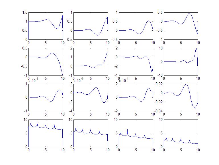
Figure 1: Smoothness Indicators, t=0.05

Example 1. In the first example, we solve Burgers’ equation

$$u_{t}+(u^{2}/2)_{x}=0$$

with the boundary condition $u_{L}(t)=1$ and initial condition

$$u_{I}(x)=1-(x/11)^{3}\sin(x)$$

in $x\in\Omega=[0,10]$. In this numerical example with $p=3$ and $k=3$, the cell size is $h=0.05$, while the time step size is $\tau_{n}=0.005$.. The solution has been computed in $t\in[0,2]$. The smoothness indicators at $t=0.05$, $t=1.05$, and $t=2.0$ are shown in Figure 1, Figure 2, and Figure 3 respectively.

In each figure, the four plots in the top row are $M^{0}_{n}(=u^{c}_{n})$, $M^{1}_{n}$, $M^{2}_{n}$, and $M^{3}_{n}$, from left to right. The index $j$ is dropped because each curve contains the values of $M^{l}_{n,j}$ for $j=0,\cdots,199$. The four plots in the second row are the temporal smoothness indicators $u^{h}_{t}(t_{n})$, $u^{h}_{tt}(t_{n})$, $u^{h}_{ttt}(t_{n})$, and $u^{h}_{tttt}(t_{n})$. The four plots in the third row are the jumps $J^{0}_{n}$, $J^{1}_{n}$, $J^{2}_{n}$, and $J^{3}_{n}$. In order to view the jumps from a better perspective, we show $\log_{h}|J^{0}_{n}|$, $\log_{h}|J^{1}_{n}|$, $\log_{h}|J^{2}_{n}|$ and $\log_{h}|J^{3}_{n}|$ in the fourth row. Since $J^{l}_{n,j}=D^{l}_{n,j}h^{p+1+\mu-l(1+\alpha)}$, the plot of $\log_{h}|J^{l}_{n,j}|=p+1+\mu-l(1+\alpha)+\log_{h}|D^{l}_{n,j}|$ reveals the order ($h^{?}$) of the jumps. Since $p,\mu$ and $\alpha$ are all known, the values of $D^{l}_{n,j}$ can be computed. Consequently, we can find $\tilde{D}$.

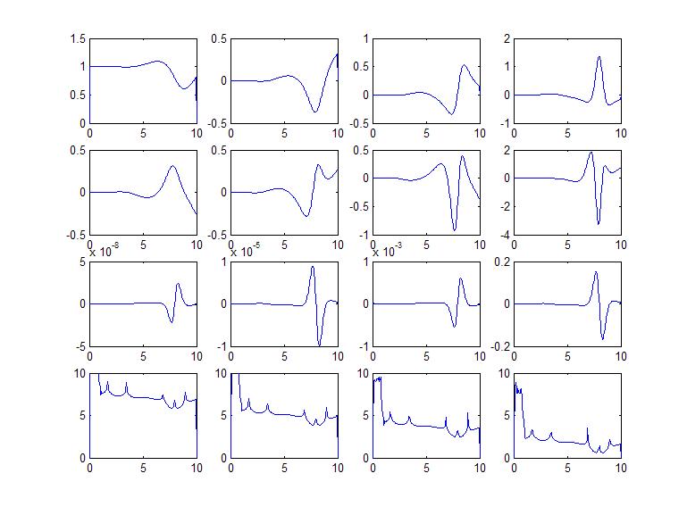
Figure 2: Smoothness Indicators, t=1.05

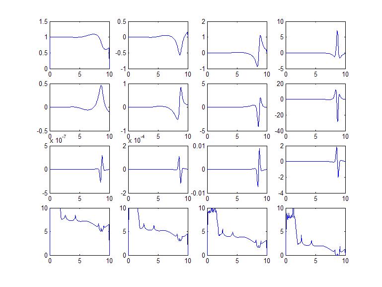
Figure 3: Smoothness Indicators, t=2.0

It is easy to see the boundedness of $M^{l}_{n}$ and $T^{3}_{n}$ in the figures when/where the solution is smooth. It is also easy to see that the order of the jumps $J^{l}_{n}$ is as expected in the error analysis, or even smaller. These observations are sufficient to support the error estimates given in the paper.

In addition, we have also observed some interesting phenomena. (1) $log_{h}|J^{0}_{n}|-log_{h}|J^{1}_{n}|\approx 2$, $log_{h}|J^{1}_{n}|-log_{h}|J^{2}_{n}|\approx 1.4$, $log_{h}|J^{2}_{n}|-log_{h}|J^{3}_{n}|\approx 1.8$. There seems to be something related to the odd or even degrees of the polynomials. (2) Long before the formation of a shock ($t=2.0$, $u_{x}\geq-0.6$), the fourth and third derivatives have grown significantly in a very narrow subdomain. The approximation benefit of the higher degree polynomials and the high order Runge-Kutta scheme will soon be lost locally at the spot. It seems that adaptive treatments need to kick in early. If not, there will be “numerical instability” showing up, ruining the numerical solution.

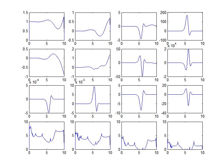
Figure 4: Smoothness Indicators, $\tau_{n}=0.0075,t=0.12$

In Figure 4, we show another numerical solution of the same problem, computed with $h=0.05$ (same as before) and $\tau_{n}=0.0075$ (50% larger). The plots are made at $t=0.12$, after 16 time steps from the initial time $t=0$. With the improperly increased time step size, although the solution (presented by $M^{0}_{n}$ in the upper left corner plot) itself has not obviously shown anything wrong from the point of view of numerical stability (boundedness of solution, TVD, etc.), the higher order derivatives and jumps in the indicators have been increased significantly. The explanation is that the RKDG scheme for this problem with $(p,k,h,\tau_{n})=(3,3,0.05,0.0075)$ does not maintain numerical smoothness. As a consequence, the optimal approximation order must have been lost. The example seems to indicate the following: the strengthened CFL condition and the numerical diffusion from the Godunov flux are needed not only for numerical stability, but also for numerical smoothness maintenance. More attention should be paid to numerical smoothness when we are concerned with high order error estimates.

The smoothness indicators can be used to diagnose the loss of numerical smoothness in an early stage, before too much damage is done to the global error. Of course, an algorithm needs to be designed for such diagnoses. We did run a separate case: after the first 5 steps at $\tau_{n}=0.0075$, $\tau_{n}$ is reduced back to $0.005$. The spurious mode created in the first 5 steps were repaired in the following steps of smaller size. Nevertheless, the damage to the global error is done, unless we redo it. Further investigation in this direction can help in finding an optimal time step size.

Example 2. In the second example, we show the solution of the Burgers’ equation on $[0,10]$ with the initial condition

$$u_{I}(x,0)=\frac{1}{2}+\frac{1}{4}\sin(\pi x/5)$$

and the periodic boundary condition. $k=3$, $p=4$, $h=0.05$, $\tau_{n}=0.005$. Figure 5 shows the numerical solution and its smoothness indicators at $t=1$, when it is still far from any shock formation.

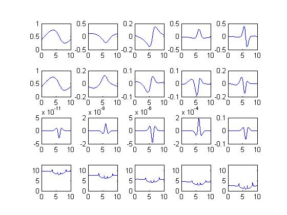
Figure 5: Smoothness Indicators, $p=4,\tau_{n}=0.005,t=1.0$

In Figure 5, the five plots in the top row are $M^{0}_{n}(=u^{c}_{n})$, $M^{1}_{n}$, $M^{2}_{n}$, $M^{3}_{n}$, and $M^{4}_{n}$, from left to right. The five plots in the second row are the temporal smoothness indicators $u^{c}_{n}$, $u^{h}_{t}(t_{n},)$, $u^{h}_{tt}(t_{n})$, $u^{h}_{ttt}(t_{n})$, and $u^{h}_{tttt}(t_{n})$. The five plots in the third row are the jumps $J^{0}_{n}$, $J^{1}_{n}$, $J^{2}_{n}$, $J^{3}_{n}$ and $J^{4}_{n}$. In the fourth row, we have $\log_{h}|J^{0}_{n}|$, $\log_{h}|J^{1}_{n}|$, $\log_{h}|J^{2}_{n}|$, $\log_{h}|J^{3}_{n}|$ and $\log_{h}|J^{4}_{n}|$. The values of the indicators are again what we expected and what we need to support the analysis. Obviously, the scheme has maintained the smoothness of the numerical solution, which guarantees that the local error of the next time step will be of optimal order.

6 Conclusion remarks

A. Choice of norm for error propagation analysis

We prefer to use the $L_{1}$-norm for error propagation analysis because of the well-known $L_{1}$-contraction property. Other than the $L_{1}$-contraction, a typical error propagation rate estimate for a time step contains a growth factor of the form $1+C\tau$. If we choose the $L_{2}$-norm for error propagation, it is easy to show that the constant $C$ is proportional to $\sqrt{|u_{x}f^{\prime\prime}(u)|}$. If we use numerical error propagation instead of PDE’s error propagation, $C$ will become bigger. “Bigger by how much” depends on the complexity of a numerical scheme. The appearance of $u_{x}f^{\prime\prime}(u)$ in the $L_{2}$-norm error propagation rate estimate implies that $L_{2}$-norm error propagation analysis based on “worst case scenario” cannot be generalized to solutions with a shock or near a shock. Since large local error is expected to appear around the self-sharpening of a solution, the real scenario of a numerical solution is probably very close to the “worst case scenario”. $L_{1}$-norm error propagation analysis does not have this difficulty.

B. How to deal with shocks and contact discontinuities?

When there is a shock or contact discontinuity, it will be detected by the smoothness indicators, as shown in [4]. Certain quantitative criteria need to be developed to determine what kind of discontinuity is present according to the behavior of the indicators. It is also needed to determine if the discontinuity is well-caught, or some level of numerical “instability” has occurred. A decision should be made on the treatment of the discontinuity, including the use of a limiter or a local front tracking technique. After all of these have been done, we can consider error estimation. Error propagation is still to be estimated by using $L_{1}$-contraction. Within each time step, in the smooth pieces of the solution, we can apply the error estimates given in this paper. At the discontinuities, we have to estimate the error according to the scheme. It is nice that the complexity of local error analysis does not get into the error propagation of the PDE.

C. The process of sharpening before shock formation may be most difficult

It might be the hardest to estimate error where a shock is forming but not yet fully developed. In this relatively wide space-time region, the solution’s high order derivatives have become larger, causing difficulties for approximation. Adaptive algorithms need to be designed, and employed according to the smoothness indicators. As seen in Figure 3 of the first numerical example, the smoothness indicators can find the local sharp growth of the higher order derivatives and their jumps. The logarithm plots of the jumps have shown a clear exclusive pattern for a point of future shock.

D. Generalization to multi-dimensional problems

We checked the proofs to the end of generalizing the results to 2-D scalar conservation laws. It seems to us that such a generalization should not meet any major difficulty. Generalization to hyperbolic systems will face the lack of $L_{1}$-contraction.

E. a posteriori vs. a priori estimates

The error analysis of this work is a posteriori because we depend on the computed smoothness indicators to compute the error estimates. However, if one can prove the boundedness of these smoothness indicators in advance, the error estimates can be converted to a priori error bounds. In this sense, under the concept of numerical smoothness, a priori and a posteriori error analysis has been united in the same framework. Moreover, our estimates are a posteriori in the sense that the smoothness indicators $S^{p}_{n}$ and $T^{k}_{n}$ are computed after $u^{c}_{n}$ has been obtained. As for the time step $[t_{n},t_{n+1}]$, the smoothness indicators needed for the local error estimates of the step are computed before the local computation toward $u^{c}_{n+1}$ has started. In this sense, our error estimation is locally a priori, which will be more efficient if adaptive treatments are desired.

F. Numerical smoothness of RKDG

In the error analysis, we actually depend on the smoothness indicators to provide the needed numerical diffusion. That is, we take advantage of the RKDG method to include the needed numerical smoothness maintenance into the error analysis. The original designers of the scheme should get the credit for inventing a scheme with such properties. Since the numerical smoothness indicators $S^{p}_{n}$ and $T^{k}_{n}$ are computed at $(t_{n},u^{c}_{n})$, Lemma 4.2 and Lemma 4.7 are needed to establish the smoothness of $\tilde{u}$ and $u^{h}$ for $t\in[t_{n},t_{n+1}]$. Lemma 4.2 shows the local smoothness preserving property of the PDE’s strong solutions (in a special case useful for the analysis). Lemma 4.7 shows the local smoothness preserving property of the semi-discrete scheme. We only need these local smoothness proofs because smoothness is only needed in dealing with local error estimates.

References

- [1] B. Cockburn, A simple introduction to error estimation for nonlinear hyperbolic conservation laws, The Graduate Student’s Guide to Numerical Analysis ’98, Springer, New York, 1999, pp.1-46.
- [2] C. Johnson and Szepessy, Adaptive finite element methods for conservation laws based on a posteriori error estimates , Comm. Pure Appl. Math. 48 (1995), pp.199–234.
- [3] P. D. Lax and R. D. Richtmyer, Survey of the stability of linear finite difference equations, Comm. Pure Appl. Math. 9 (1956), pp.267–293.
- [4] D. Rumsey and T. Sun, A smoothness/shock indicator for RK-DG on nonlinear conservation laws, Applied Math. Letters, 23 (2010), 1425-1431.
- [5] C.-W. Shu, Discontinuous Galerkin methods: general approach and stability, Numerical Solutions of Partial Differential Equations, S. Bertoluzza, S. Falletta, G. Russo and C.-W. Shu, Advanced Courses in Mathematics CRM Barcelona, Birkhauser, Basel, 2009, pp. 149-201.
- [6] J. Smoller, Shock Waves and Reaction-Diffusion Equations, Springer-Verlag, New York, 1994.
- [7] T. Sun, Stability and error analysis on partially implicit schemes, Numerical Methods for Partial Differential Equations, 21 (2005), pp.843-858.
- [8] T. Sun and D. Fillipova, Long-time error estimation on semi-linear parabolic equations, Journal of Computational & Applied Mathematics, 185 (2006), pp.1-18.
- [9] Q. Zhang and C.-W. Shu, Error estimates to smooth solutions of Runge-Kutta discontinuous Galerkin methods for scalar conservation laws , SIAM Journal on Numerical Analysis, v42 (2004), pp.641-666.
- [10] Q. Zhang and C.-W. Shu, Stability analysis and a priori error estimates to the third order explicit Runge-Kutta discontinuous Galerkin Method for scalar conservation laws, SIAM Journal on Numerical Analysis, v48 (2010), pp.1038-1063.