Time variability in simulated ultracompact and hypercompact HII regions

Abstract

Ultracompact and hypercompact H II regions appear when a star with a mass larger than about 15 solar masses starts to ionize its own environment. Recent observations of time variability in these objects are one of the pieces of evidence that suggest that at least some of them harbor stars that are still accreting from an infalling neutral accretion flow that becomes ionized in its innermost part. We present an analysis of the properties of the H II regions formed in the 3D radiation-hydrodynamic simulations presented by Peters et al. as a function of time. Flickering of the H II regions is a natural outcome of this model. The radio-continuum fluxes of the simulated H II regions, as well as their flux and size variations are in agreement with the available observations. From the simulations, we estimate that a small but non-negligible fraction ($\sim 10~{}\%$) of observed H II regions should have detectable flux variations (larger than $10~{}\%$) on timescales of $\sim 10$ years, with positive variations being more likely to happen than negative variations. A novel result of these simulations is that negative flux changes do happen, in contrast to the simple expectation of ever growing H II regions. We also explore the temporal correlations between properties that are directly observed (flux and size) and other quantities like density and ionization rates.

1 Introduction

The most massive stars in the Galaxy, O-type stars with masses $M_{\star}>20~{}M_{\odot}$, emit copious amounts of UV photons (Vacca et al., 1996) that ionize part of the dense gas from which they form. The resulting H II regions are visible via their free-free continuum and recombination line radiation (Mezger & Henderson, 1967; Wood & Churchwell, 1989). H II regions span orders of magnitude in size, from giant ($D\sim 100$ pc) bubbles, to “ultracompact” (UC) and “hypercompact” (HC) H II regions, loosely defined as those with sizes of $\sim 0.1$ pc and $\sim 0.01$ pc (or less), respectively (see the reviews by Churchwell, 2002; Kurtz, 2005; Hoare et al., 2007). UC and HC H II regions are the most deeply embedded, and so are best observed at radio wavelengths.

Large, rarefied H II regions expand without interruption within the surrounding medium due to the high pressure contrast between the ionized and neutral phases (Spitzer, 1978). This simple model was extrapolated to the ever smaller objects recognized later and is widely used to interpret observations of UC and HC H II regions. Common assumptions about these objects are: i) They are steadily expanding within their surrounding medium at the sound speed of the ionized gas, $\sim 10$ ${\rm~{}km~{}s}^{-1}$. ii) The ionizing star(s) is already formed, i.e., accretion to the massive star(s) powering the H II region has stopped.

However, evidence has accumulated that suggests a revision of these assumptions:

1. The “hot molecular cores” embedding UC and HC H II regions are often rotating and infalling (e.g., Keto, 1990; Cesaroni et al., 1998; Beltrán et al., 2006, 2010; Klaassen et al., 2009), sometimes from parsec scales all the way to the immediate surroundings of the ionized region (Galván-Madrid et al., 2009; Baobab Liu et al., 2010).

2. Infall of gas at velocities of a few ${\rm~{}km~{}s}^{-1}$ directly toward the ionized center has also been observed in UC and HC H II regions (Zhang & Ho, 1997; Beltrán et al., 2006; Galván-Madrid et al., 2009).

3. The inner ionized gas has been resolved in a few cases, and it also shows accretion dynamics (outflow, infall, and rotation, e.g., Keto & Wood, 2006; Sewiło et al., 2008; Galván-Madrid et al., 2009).

4. The spectral index $\alpha$ (where the flux goes as $S_{\nu}\propto\nu^{\alpha}$) of some UC and HC H II regions is $\sim 1$ from cm to mm wavelengths, indicating density gradients and/or clumpiness inside the ionized gas (Franco et al., 2000; Ignace & Churchwell, 2004; Keto et al., 2008; Avalos et al., 2009).

5. A few UC and HC H II regions have been shown to have variations on timescales of years (Acord et al., 1998; Franco-Hernández & Rodríguez, 2004; van der Tak et al., 2005; Galván-Madrid et al., 2008). These variations indicate that UC and HC H II regions sometimes expand (Acord et al., 1998), and sometimes contract (Galván-Madrid et al., 2008). Some other ionized regions around massive protostars have been shown to remain approximately constant in flux (Goddi et al., 2011).

All these observations strongly suggest that UC and HC H II regions are not homogeneous spheres of gas freely expanding into a quiescent medium, but rather that these small H II regions are intimately related to the accretion processes forming the massive stars. Simple analytic models show that the observed H II region can be either the ionized, inner part of the inflowing accretion flow (Keto, 2002, 2003) or the ionized photoevaporative outflow (Hollenbach et al., 1994) fed by accretion (Keto, 2007).

Numerical simulations of the formation and expansion of H II regions in accretion flows around massive stars have only recently become possible with three-dimensional radiation-hydrodynamics. Studies that simulate the expansion of H II regions have focussed on larger-scale effects on the parental molecular cloud (Dale et al., 2005, 2007a, 2007b; Peters et al., 2008; Gritschneder et al., 2009; Arthur et al., 2011). However, in none of those simulations was the ionizing radiation produced by the massive stars dynamically forming through gravitational collapse in the molecular cloud. Recent simulations by Peters et al. (2010a) (hereafter Paper I) include a more realistic treatment of the formation of the star cluster. Radio-continuum images generated from the output of the simulations of Paper I show time variations in the morphology and flux from the H II regions produced by the massive stars in formation. These changes are the result of the complex interaction of the massive filaments of neutral gas infalling to the central stars with the ionized regions produced by some of them. A statistical analysis of the H II region morphologies (Peters et al., 2010b, Paper II) consistently reproduces the relatively high fraction of spherical and unresolved regions found in observational surveys. Thus, the non-monotonic expansion of H II regions, or flickering, appears able to resolve the excess number of observed UC and HC H II regions with respect to the expectation if they expand uninterrupted (the so-called lifetime problem, Wood & Churchwell, 1989). Furthermore, the ionizing radiation is unable to stop protostellar growth when accretion is strong enough. Instead, accretion is stopped by the fragmentation of the gravitationally unstable accretion flow in a process we call “fragmentation-induced starvation”, a theoretical discussion of which can be found in Peters et al. (2010c) (Paper III).

In this paper we present a more detailed analysis of the flux variability in the simulations presented in Paper I. In §2 we describe the set of numerical simulations and the methods of analysis. In §3 we present our results. §4 discusses the implications of our findings. In §5 we present our conclusions.

2 Methods

2.1 The Numerical Simulations

Our study uses the highest resolution simulations of those presented in Paper I. The simulations use a modified version of the adaptive-mesh code FLASH (Fryxell et al., 2000), including self-gravity and radiation feedback. They include for the first time a self-consistent treatment of gas heating by both ionizing and non-ionizing radiation. We refer the reader to Paper I for further details of the numerical methods. The initial conditions are a cloud mass of 1000 $M_{\odot}$ with an initial temperature of 30 K. The initial density distribution is a flat inner region of 0.5 pc radius surrounded by a region with a decreasing density $\propto r^{-1.5}$. The density in the homogeneous volume is $1.27\times 10^{-20}$ g cm^-3. The simulation box has a length of 3.89 pc. The size and mass of the cloud are in agreement with those of star-formation regions that are able to produce at least one star with $M_{\star}>20~{}M_{\odot}$ (e.g., Galván-Madrid et al., 2009).

Run A (as labeled in Paper I) has a maximum cell resolution of 98 AU and only the first collapsed object is followed as a sink particle (see Federrath et al., 2010). In this run, the formation of additional stars (the sink particles) is suppressed using a density-dependent temperature floor (see Paper I for details). On the other hand, in run B additional collapse events are permitted and a star cluster is formed, each star being represented by a sink particle. The maximum resolution in Run B is also 98 AU.

2.2 Data Sets

For the entire time span of Run A (single sink) and Run B (multiple sink), radio-continuum maps at a wavelength of 2 cm were generated from the simulation output every $\sim 300$ yr by integrating the radiative transfer equation for free-free radiation while neglecting scattering (Gordon & Sorochenko, 2002). Following Mac Low et al. (1991), each intensity map was then convolved to a circular Gaussian beam with half-power beam width HPBW $=0.14^{\prime\prime}$ (assuming a source distance of 2.65 kpc). A noise level of $10^{-3}$ Jy was added to each image. Further details are given in Paper I. These maps were used to explore the behavior of the free-free continuum from the H II region over the entire time evolution of the simulations. For Run B, sometimes the H II regions overlap both physically in space and/or in appearance in the line of sight. Therefore, the presented time analysis refers to the entire star cluster unless otherwise specified.

To compare more directly to available observations, which span at most a couple of decades in time, each of Run A and B were re-run in four time intervals for which a flux change was observed in the radio-continuum images mentioned above. Data dumps and radio-continuum maps were generated at every simulation time step ($\sim 10$ yr). The analysis performed in the low time-resolution maps was also done in these high time-resolution data. For Run B, the intervals for the high time-resolution data were also selected such that the H II region powered by the most massive star is reasonably isolated from fainter H II regions ionized by neighboring sink particles, both in real space and in the synthetic maps.

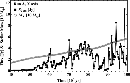
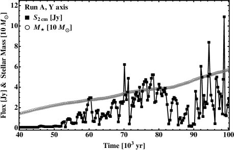
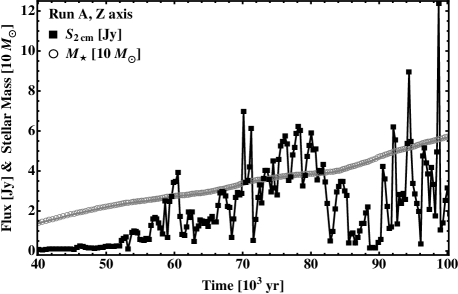
Figure 1: 2-cm flux ($S_{\rm 2cm}$, filled black squares) and stellar mass ($M_{\star}$, gray circles) as a function of time ($t$) for Run A. Although the long-term trend of the H II region is to increase in flux, it constantly flickers during its evolution. The fluxes at the different projections (X-axis top, Y-axis middle, Z-axis bottom), though not the same, follow each other closely.

3 Results

3.1 Variable HII Regions

Real UC and HC H II regions, as well as those that result from the simulations presented here, are far from the ideal cases (e.g., Spitzer, 1978). However, it is instructive to discuss the limiting ideal cases to show that their variability is a natural consequence of their large to moderate optical depth.

The flux density $S_{\nu}$ of an ionization-bounded H II region is

$$S=\frac{2k\nu^{2}}{c^{2}}\int_{\Omega}T_{\mathrm{B}}d\Omega,$$ (1)

where $k$ is the Boltzmann constant, $c$ is the speed of light, $\nu$ is the frequency, and the brightness temperature $T_{\mathrm{B}}$ is integrated over the angular area $\Omega$ of the H II region.

In the limit of very low free-free optical depths ($\tau_{\mathrm{ff}}\ll 1$), $T_{\mathrm{B}}$ along a line of sight $l$ goes as

$$T_{\mathrm{B}}\propto T_{e}^{-0.35}\nu^{-2.1}\int_{l}n^{2}dl,$$ (2)

where $T_{e}$ and $n$ are the electron temperature and density respectively.

Combining equations (1) and (2) we have that for a given $\nu$ and constant $T_{e}$:

$$S(\tau_{\mathrm{ff}}\ll 1)\propto n^{2}R^{3}\propto\dot{N},$$ (3)

where the last proportionality comes from the Strömgren relation $\dot{N}\propto n^{2}R^{3}$ ($\dot{N}$ is the ionizing-photon rate and $R$ is the ‘radius’ of the H II region). Equation (3) shows that in the optically-thin limit the H II -region flux only depends on $\dot{N}$. For time intervals of a few $\times 10$ yr the mass and ionizing flux of an accreting protostar remain almost constant, and so does the flux of an associated optically-thin H II region.

On the other hand, for very high optical depths ($\tau_{\mathrm{ff}}\gg 1$) $T_{\mathrm{B}}=T_{e}$. For a given frequency and constant $T_{e}$, equation (1) becomes:

$$S(\tau_{\mathrm{ff}}\gg 1)\propto R^{2}\propto\dot{N}^{2/3}n^{-4/3},$$ (4)

therefore, the flux of an optically thick H II region is proportional to its area, and both flux and area decrease with density.

This analysis is valid for time intervals larger than the recombination timescale ($\sim 1$ month for $n\sim 10^{6}$ cm^-3, see e.g., Osterbrock, 1989) and as long as the growth of $\dot{N}$ is negligible.

However, the H II regions in the simulations are clumpy and have subregions of high and low free-free optical depth. Their flux during the accretion stage (while they flicker) is dominated by the denser, optically thicker ($\tau_{\mathrm{ff}}>1$) subregions, so their behaviour is closer to eq. (4) than to eq. (3). The on-line version of this paper contains a movie of $\tau_{ff}$ for Run B as viewed from the Z-axis (line of sight perpendicular to the plane of the accretion flow). The clumpiness and intermediate-to-large optical depth of these H II regions are also the reasons behind their rising spectral indices up to relatively large frequencies ($\nu>100$ GHz) without a significant contribution from dust emission (see the analytical discussions of Ignace & Churchwell 2004 and Keto et al. 2008, for an analysis of these simulations see Paper II). As for the variability, the large optical depths cause the size and flux of the simulated H II regions to be well correlated with each other, and anticorrelated with the density of the central ionized gas (see Section 3.6). The neutral accretion flow in which the ionizing sources are embedded is filamentary and prone to gravitational instability (further discussion is in Section 3 of Paper III, see also Paper II). The changes in the density of the H II regions are a consequence of their passage through density enhancements in the quickly evolving accretion flow.

3.2 Global Temporal Evolution

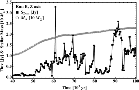
Figure 2: 2-cm flux ($S_{\rm 2cm}$, filled black squares) of the H II region formed by the most massive star and its stellar mass ($M_{\star}$, gray circles) as a function of time ($t$) for Run B. Although the long-term trend of the H II region is to increase in flux, it constantly flickers during its evolution. Only the Z-axis projection is used because from this viewing angle, perpendicular to the plane of the accretion flow, the brightest H II region can be distinguished from other H II regions at all times.

Figure 3: 2-cm flux variations ($\Delta S_{\rm 2cm}$) for Run A (top panel) and Run B (bottom) panel.

Figure 1 shows the global temporal evolution of the H II region in Run A (single sink particle). The 2-cm flux ($S_{\rm 2cm}$) observed from orthogonal directions and the mass of the ionizing star ($M_{\star}$) are plotted against time. The global temporal trend of the H II region is to expand and become brighter. However, fast temporal variations are seen at all the stages of the evolution. The fluxes in the projections along the three different cartesian axes follow each other closely. For the rest of the analysis, the Z-axis projection, a line of sight perpendicular to the plane of the accretion flow, is used.

Figure 4: Fractional flux variations ($\Delta S_{\rm 2cm}/S_{\rm 2cm,0}$) for Run A (top panel) and Run B (bottom) panel.

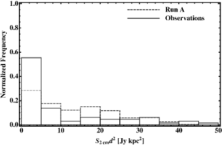
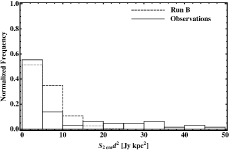
Figure 5: Histograms of 2-cm luminosities ($S_{\rm 2cm}d^{2}$) for the global temporal evolution of the simulated H II regions (dashed lines) and the co-added samples of Wood & Churchwell (1989) and Kurtz et al. (1994) (solid lines). The top and bottom frames correspond to Run A and Run B respectively.

The H II region is always faint ($S_{\rm 2cm}<1$ Jy at the assumed distance of 2.65 kpc) for $M_{\star}<25~{}M_{\odot}$. Past this point, the H II region is brighter than 1 Jy 86 % of the time (Fig. 1).

Figure 6: Probabilities for flux increments larger than 10 (top panel), 50 (middle), and $90~{}\%$ (bottom) as a function of time difference for the long-term evolution of the H II region in Run A. The error bars indicate the $1\sigma$ statistical uncertainty from the number of counts in each bin 1000-yr wide.

Figure 7: Probabilities for flux increments larger than 10 (top panel), 50 (middle), and $90~{}\%$ (bottom) as a function of time difference for the long-term evolution of the H II regions in Run B. The error bars indicate the $1\sigma$ statistical uncertainty from the number of counts in each bin 1000-yr wide.

Figure 8: Probabilities for flux decrements larger than 10 (top panel), 50 (middle), and $90~{}\%$ (bottom) as a function of time difference for the long-term evolution of the H II region in Run A. The error bars indicate the $1\sigma$ statistical uncertainty from the number of counts in each bin 1000-yr wide.

Figure 9: Probabilities for flux decrements larger than 10 (top panel), 50 (middle), and $90~{}\%$ (bottom) as a function of time difference for the long-term evolution of the H II regions in Run B. The error bars indicate the $1\sigma$ statistical uncertainty from the number of counts in each bin 1000-yr wide.

A similar analysis of the H II region around the most massive star in Run B (multiple sinks) is shown in Fig. 2. Only the Z-axis projection, i.e., a line of sight perpendicular to plane of the accretion flow is used, since only from this viewing angle the brightest H II region is well separated from other H II regions at all times (the flux movies are presented in Paper I). The extra fragmentation in Run B translates into a weaker accretion flow and a lower-mass ionizing star as compared to that of Run A, a process referred to as ’fragmentation-induced starvation’ (a theoretical discussion of this process in presented in Paper III). Therefore, the brightest H II region in Run B (Fig. 2) is weaker than the H II region in Run A (Fig. 1). Figures 1 and 2 do not show times later than $t=100$ kyr in order to facilitate their comparison. Both runs continue past this time, but in Run B accretion onto the most massive star stops at $t=109$ kyr, while in Run A the artificial suppression of the fragmentation leads to an unrealistically large mass for the ionizing star at later times (see Paper I).

H II regions are highly variable both in Run A and Run B. However, since the suppression of fragmentation in Run A produces a larger accretion flow and a most massive ionizing star, Run A presents larger flux variations than Run B. Figure 3 shows the flux changes over the evolution of the H II regions in both runs. A comparison of the fractional variations of the H II regions shows that, though more similar between runs, they are still larger in Run A (Figure 4). For consecutive data points, in Run A positive flux variations are 56 % of the events and the flux increment is $+74$ % on average, while negative changes are 44 % of the events and have an average magnitude of $-27$ %. Similarly, for Run B, positive changes (52 % of the events) have an average magnitude of $+42$ %, while the average flux decrement (48 % of the events) is $-18$ %.

3.3 Comparison to Surveys

We present a comparison with the ionized-gas surveys of UC and HC H II regions by Wood & Churchwell (1989) and Kurtz et al. (1994). Figure 5 shows normalized histograms of 2-cm luminosity ($S_{\rm 2cm}d^{2}$) obtained for both runs using the time steps previously shown in figures 1 to 4 and the co-added observed samples from Wood & Churchwell (1989) and Kurtz et al. (1994), taking the 81 sources for which they report a 2-cm flux and a distance. Simulation and observations roughly agree, but neither Run A nor B can reproduce the high-luminosity end of the observed distribution: 20 % of the observed sources have $S_{\rm 2cm}d^{2}>50$ Jy kpc², while only 1 % of the H II regions in the simulation steps of Run A and in no step in Run B have luminosities above this threshold. These bright UC H II regions likely correspond to stages in which accretion to the ionizing protostar(s) is completely shut off, therefore they do not correspond to the analyzed H II regions from the simulation in which the protostars are still accreting. In the range $20<S_{\rm 2cm}d^{2}<50$ Jy kpc², Run A matches better than Run B the observed luminosities. This may be because Run B does not produce any star with a mass $M_{\star}>30~{}M_{\odot}$. Simulations identical to Run B produce higher-mass stars in the presence of magnetic fields (Peters et al., 2011) and may also produce more massive stars in the purely radiation-hydrodynamical case with higher-mass initial clumps. We plan to perform in the future a study on the robustness of our results for different initial conditions. For the smallest luminosities, Run B matches better than Run A the observed 55 % of H II regions that have $S_{\rm 2cm}d^{2}<5$ Jy kpc², but over-estimates (35 %) the observed fraction (14 %) of H II regions with $5<S_{\rm 2cm}d^{2}<10$. Peters et al. (2010b) presented statistics of the morphologies of the H II regions in Run A and Run B and found that Run B agrees better with observed surveys. Although Run A can be interpreted as a mode of isolated massive star formation, the treatment of fragmentation is more realistic in Run B (see Paper I). Moreover, most high-mass stars form in clusters (Zinnecker & Yorke, 2007).

3.4 Long-Term Variation Probabilities

We address the question of the flux variability expected from the simulations by calculating the probability of variations larger than a given threshold as a function of time difference between steps. The low time-resolution data has the advantage of spanning the entire runs, but is not useful to predict the expected variations on timescales shorter than $10^{2}$ yr. We use the high time-resolution data sets to make an estimate of the flux variations over shorter timescales, but we caution that the analyzed time intervals may not be representative of the entire simulation. We use this approach because re-running the entire simulations to produce data at $\sim 10$ yr resolution is not feasible.

Figures 6 and 7 show the probabilities of flux increments larger than a given threshold for time differences between 1 and 60 kyr for Run A and Run B respectively. The top panels correspond to flux increments larger than $10~{}\%$, the middle panels correspond to $50~{}\%$, and the bottom panels to $90~{}\%$. On average, H II regions tend to expand, making a given flux increment to be more likely to happen for larger time intervals than for shorter ones.

Figures 8 and 9 show the probabilities of flux decrements larger than a given threshold (in modulus) for Run A and Run B respectively. At $\Delta t>30$ kyr the negative-change probabilities decrease and reach $\sim 0$ at about $\Delta t>40$ kyr for any threshold. This is caused by the eventual growth of the H II regions in spite of the flickering. There is some indication that the probabilities for negative changes also decrease at timescales shorter than 1 kyr, specially for flux-change thresholds larger than $50~{}\%$ (see Figs. 8 and 9). This is also suggested from the analysis of the high temporal-resolution data in the next section. Although flux increments are more likely than decrements for any given threshold and time lag, a novel result of these simulations is that negative flux changes do happen, in contrast with the simple expectation of ever growing H II regions.

3.5 Short-Term Variation Probabilities

Figure 10: Probabilities for flux increments larger than 10 (top panel), 50 (middle), and $90~{}\%$ (bottom) as a function of time difference for the sample intervals at high time resolution. The error bars indicate the $1\sigma$ statistical uncertainty from the number of counts in each bin 20-yr wide.

Figure 11: Probabilities for flux increments larger than 10 (top panel), 50 (middle), and $90~{}\%$ (bottom) as a function of time difference for the sample intervals at high time resolution, for Run B. The error bars indicate the $1\sigma$ statistical uncertainty from the number of counts in each bin 20-yr wide.

Figure 12: Probabilities for flux decrements larger than 10 (top panel), 50 (middle), and $90~{}\%$ (bottom) as a function of time difference for the sample intervals at high time resolution. The error bars indicate the $1\sigma$ statistical uncertainty from the number of counts in each bin 20-yr wide.

Figure 13: Probabilities for flux decrements larger than 10 (top panel), 50 (middle), and $90~{}\%$ (bottom) as a function of time difference for the sample intervals at high time resolution, for Run B. The error bars indicate the $1\sigma$ statistical uncertainty from the number of counts in each bin 20-yr wide.

We re-ran four time intervals in each of Run A and Run B, spanning a few hundred years each, and producing data dumps at each simulation step ($\sim 10$ yr). These time intervals were selected to contain a pair of negative/positive flux changes to investigate the correlation of flux variations with physical changes in the H II region, like size and density (next section). Therefore, they may not be representative of the entire simulation, but since it is not feasible to re-run the entire simulations producing data dumps at the highest temporal resolution, we use these data to constrain the expected flux variations in observable timescales. We argue that the close match at scales of $\Delta t\sim 500$ yr between the probabilities obtained from the low temporal-resolution (previous section) and the high temporal-resolution data (this section) indicates that the results presented here are meaningful.

Figures 10 and 11 show, for Run A and Run B respectively, the probabilities for flux increments larger than the specified threshold as a function of time lag. These figures are the analogs of Figs. 6 and 7 for the high temporal-resolution data. The slight probability decrements after $\Delta t\sim 300$ yr, especially at low thresholds, are an artifact caused by the fact that the data sets include a negative/positive flux-change pair. Still, the probabilities at $\Delta t=490$ yr match within 20 % to 80 % with the probabilities at $\Delta t=500$ yr from the low-temporal resolution data.

On observable timescales, $\Delta t=0$ to 40 yr, a small but non-zero fraction of H II regions is expected to have detectable flux increments. For two observations separated by $10$ yr, Run A gives a prediction of $16.7\pm 2.9~{}\%$ of H II regions having flux increments larger than 10 %, $6.8\pm 1.9~{}\%$ with flux increments larger than 50 %, and $4.7\pm 1.6~{}\%$ with increments larger than 90 %. The more realistic Run B predicts a smaller fraction of variable H II regions: $6.9\pm 1.6~{}\%$, $0.3\pm 0.3~{}\%$, and $0~{}\%$ of them are expected to have flux increments larger than 10 %, 50 %, and 90 % over a time interval of $10$ yr, respectively.

Figures 12 and 13 show the probabilities for flux decrements larger than a given threshold obtained with the high temporal-resolution data. The probabilities obtained at $\Delta t=490$ yr from the high temporal-resolution data roughly match with those at $\Delta t=500$ yr obtained from the low temporal-resolution data, within a factor of 1 to 3.

Negative variations should also be detectable in a non-negligible fraction of H II regions. Run A predicts that $5.7\pm 1.7~{}\%$, $2.6\pm 1.2~{}\%$, and $1.6\pm 0.1~{}\%$ of H II regions should present flux decrements larger than 10 %, 50 %, and 90 % respectively, when observed in two epochs separated by $10$ yr. Run B predicts a smaller fraction of H II regions with negative flux variations: $3.3\pm 1.1~{}\%$, $1.5\pm 0.7~{}\%$, and $0~{}\%$ for thresholds at 10 %, 50 %, and 90 % respectively. We emphasize that negative variations are not expected in classical models of monotonic H II region growth, while they are a natural outcome of the model presented here. Moreover, these variations should be detectable with current telescopes.

3.6 Variations in other properties of the HII regions

Because Run B is more realistic in the treatment of fragmentation (Section 2.1, see Paper I for details), we use the time intervals of Run B with data at high temporal resolution to investigate the correlations of sudden flux changes with other properties of the H II regions.

Let the size of the H II region of interest be defined as $L_{\mathrm{HII}}=2(A/\pi)^{1/2}$, where $A$ is the area in the synthetic image where the H II region is brighter than three times the rms noise. Lets also consider the average density of the H II region $\rho_{\mathrm{HII}}$, and the rate at which neutral gas is converted into ionized gas $\dot{M}_{\mathrm{\rightarrow HII}}$. Figure 14 compares the time evolution of these three quantities.

Figure 15 further compares the time evolution of the 2-cm flux $S_{\mathrm{2cm}}$, the total ionized mass $M_{\mathrm{HII}}$ in the H II region, and the denser ionized mass within the same volume $M_{\mathrm{HII,dense}}$. The density threshold to define this dense gas is $\rho_{\mathrm{HII}}>10^{-17}$ g cm^-3, the typical peak density reached when the H II region gets rapidly denser immediately after the flickering events (see Fig. 14).

The flux-size correlation, as well as the size-density anticorrelation are a consequence of the relatively large optical depths of the H II regions (see Section 3.1). The “quenching” events, when an H II region has a large, sudden drop in flux and size, are coincident with large increments in the ionized density. The H II region rapidly reaches a state close to ionization equilibrium at its new size after the quenching instability. In Fig. 14 it is seen that at the moment of the quenching, the ionization rate has a sharp decrement immediately followed by an even faster increment that marks the initial re-growth of the H II region. Shortly afterwards, the ionization rate stabilizes again and the H II region grows hydrodynamically, gradually becoming larger and less dense.

The ionized mass of the H II regions follows the flux and size closely (Fig. 15), since this is the gas responsible for the free-free emission. However, if only the denser gas is taken into account, the amount of this dense ionized gas is particularly high in the initial re-growth of the H II region immediately after the quenching event (Fig. 15). Therefore the rapid quenching events are marked by the presence of denser gas around the accreting massive protostar.

4 Discussion

4.1 A new view of early H II region evolution

Until recently, H II regions have been modeled as (often spherical) bubbles of ionized gas freely expanding into a quiescent medium. However, this paradigm fails to explain observations of some UC and HC H II regions (see Section 1). There is enough evidence to assert that massive stars form in clusters by accretion of gas from their complex environment (reviews have been presented by Garay & Lizano, 1999; Mac Low & Klessen, 2004; Beuther et al., 2007; Zinnecker & Yorke, 2007). Centrally peaked, anisotropic density gradients are expected at the moment an accreting massive star starts to ionize its environment. Therefore, the earliest H II regions should not be expected to be the aforementioned bubbles, but more complex systems where ionized gas that is outflowing, rotating, or even infalling may coexist. The feasibility of this scenario has been shown by analytic models (Hollenbach et al., 1994; Keto, 2002, 2003, 2007; Lugo et al., 2004) and recent numerical simulations (Papers I, II, and III). In these numerical models, the inner part of the accretion flow is mostly ionized, while the outer part is mostly neutral. The neutral accretion flow continuously tries to feed the central stars. The interaction of this infalling neutral gas with the ionized region has a remarkable observational effect: the flickering of the free-free emission from the H II region.

We stress that the flickering is not a gasdynamical effect. Instead, it is a non-local result of the shielding of the ionizing source by its own accretion flow. Hence, variations in the ionization state of the gas inside the H II region are not limited by the speed of sound but can happen on the much shorter recombination timescale of the ionized gas, rendering direct observation of this flickering effect feasible.

Figure 14: Variation at high temporal resolution in Run B of the scale length $L_{\mathrm{HII}}$ (filled black circles) of the H II region around the most massive sink particle, its average density $\rho_{\mathrm{HII}}$ (filled black squares), and its rate of ionization of neutral gas $\dot{M}_{\mathrm{\rightarrow HII}}$ (filled black diamonds).

Figure 15: Variation at high temporal resolution in Run B of the 2-cm flux $S_{\mathrm{2cm}}$ (filled black circles) of the H II region around the most massive sink particle, its ionized mass $M_{\mathrm{HII}}$ (filled black squares), and its dense-gas ionized mass $M_{\mathrm{HII,dense}}$ (filled black diamonds)

.

4.2 Observational Signatures

Time-variation effects are expected in the ionized gas but not in the molecular gas, since small clumps of molecular gas that become ionized and/or recombine have a much larger effect on the emission of the $<1~{}M_{\odot}$ of ionized gas than on the tens to hundreds of $M_{\odot}$ of molecular gas in the accretion flow. One observational example is the HC H II region G20.08N A, for which Galván-Madrid et al. (2009) reports an ionized mass of $0.05~{}M_{\odot}$ and a mass of warm molecular gas in the inner 0.1 pc of 35 to 95 $M_{\odot}$ (another well studied example is G10.6–0.4, with more than $1000~{}M_{\odot}$ in the pc-scale molecular flow surrounding the H II regions, e.g., Keto, 1990; Keto & Wood, 2006; Liu et al., 2011, and references therein). The H II regions in the simulations also have masses of ionized gas in the range $10^{-3}$ to $10^{-1}~{}M_{\odot}$ while the stars are still accreting.

In sections 3.4 and 3.5 we have attempted to quantify the expected flux variations in the radio continuum of H II regions for massive stars forming in isolation (Run A) and, more realistically, in clusters (Run B). The accretion flow in Run A is stronger than in Run B (actually the star in Run A never stops accreting, see Papers I and III), which leads to a brighter and more variable H II region.

For a given run, flux variation threshold, and time difference, positive variations are more likely to happen than negative ones, i.e., there is a constant struggle between the H II region trying to expand and the surrounding neutral gas trying to confine it, with a statistical bias toward expansion.

Monitoring H II regions for thousands of years is not possible, but a few observations of rapid flux changes over timescales of $\sim 10$ yr have been presented in the literature (Acord et al., 1998; Franco-Hernández & Rodríguez, 2004; van der Tak et al., 2005; Galván-Madrid et al., 2008). Comparing multi-epoch images made with radio-interferometers can be challenging: even if the absolute flux scale of the standard quasars is known to better than $2~{}\%$, slight differences in observational parameters between observations (mainly the Fourier-space sampling, see Perley et al., 1989) make questionable any observed change smaller than $10~{}\%$. We have therefore measured the variation probabilities in the simulations at thresholds starting at $10~{}\%$. Considering this detection limit for the more realistic case of Run B, we have estimated that about $7~{}\%$ of UC and HC H II regions observed at two epochs separated by about 10 years should have detectable flux increments, and that about $3~{}\%$ should have detectable decrements. In total, $\sim 10~{}\%$ of H II regions should have detectable flux variations in a period of 10 years. Dedicated observations of as many sources as possible are now needed to test this model.

Our long timescale data can only be constrained by observational surveys, not by time monitoring. In Section 3.3 we have shown that the radio luminosities (i.e., distance-corrected flux) in the long-term evolution of the simulated H II regions are consistent with major surveys, except for the most luminous H II regions, in which likely accretion has stopped and which therefore do not correspond with our data. The hypothesis that a considerable fraction of observed UC and HC H II regions may harbor stars that are still accreting material still needs more convincing evidence in addition to matching the model here presented. For most cases the dynamics of the surrounding molecular gas and of the ionized gas have not been studied at high angular resolution, and such studies in many sources are key to test this idea. From available observations, almost all of the massive star formation regions with signatures of active accretion and in which the mass of the protostar is estimated from dynamics to be $M_{\star}>20~{}M_{\odot}$ have a relatively bright H II region (with at least $\sim 100$ mJy at short cm wavelenghts, e.g., Beltrán et al., 2007; Galván-Madrid et al., 2009). To our knowledge, the only clear exception is the recent report by Zapata et al. (2009) of an accreting protostar in W51 N with an estimated mass of $M_{\star}\sim 60~{}M_{\odot}$ and only 17 mJy at 7 mm. This object can be understood in the context of our simulations if it is in a quenched, faint state as currently observed.

4.3 Caveats and limitations

As mentioned in Papers I, II, and III, the simulations here presented do not include the effects of stellar winds and magnetically-driven jets originating from within 100 AU, which would produce outflows that are more powerful than the purely pressure-driven outflows that appear in Runs A and B (Paper I).

The inclusion of stellar winds and jets may affect the results presented in this paper only quantitatively. Peters et al. (2011) have shown that magnetically driven outflows from radii beyond 100 AU do not stop accretion and even channel more material to the central most massive protostars. The simulations of Wang et al. (2010) also indicate that collimated outflows may be an important regulator of star formation by slowing the accretion rate but without impeding accretion. Observationally, molecular outflows tend to be less collimated for the more massive O-type protostars capable of producing H II regions than for B-type protostars (Arce et al., 2007). Regarding the radio-continuum, it is unknown if the free-free emission from the photoionized H II regions produced by O-type protostars can coexist with the free-free emission from (partially) ionized, magnetically driven jets. Before the appearance of an H II region, these jets are detected in protostars less massive than $\sim 15~{}M_{\odot}$ (e.g., Carrasco-González et al., 2010), and even though their radio emission also appears to be variable (due to motions and interactions with the medium, e.g., Curiel et al., 2006), their typical centimeter flux is $\sim 1$ mJy, one to two orders of magnitude fainter than the typical flux of UC and HC H II regions (except maybe for the youngest gravitationally-trapped H II regions, see Keto, 2003). Therefore, the relative effect of any variation in a hypothetical radio jet should be small compared with the variations in the H II region flux.

A further limitation of this study is that accretion onto the protostars is not well resolved, since the maximum cell resolution (98 AU) corresponds to a scale of the order of the inner accretion disk (see also Paper I).

5 Conclusions

We performed an analysis of the radio-continuum variability in H II regions that appear in the radiation-hydrodynamic simulations of massive-star formation presented in Paper I. The ultimate fate of ultracompact and hypercompact H II regions is to expand, but during their evolution they flicker due to the complex interplay of the inner ionized gas and the outer neutral gas. The radio-luminosities of the H II regions formed by the accreting protostars in our simulations are in agreement with those of observational radio surveys, except for the most luminous of the observed H II regions. We show that H II regions are highly variable in all timescales from 10 to $10^{4}$ yr, and estimate that at least $10~{}\%$ of observed ultracompact and hypercompact H II regions should exhibit flux variations larger than $10~{}\%$ for time intervals longer than about 10 yr.

References

- Acord et al. (1998) Acord, J. M., Churchwell, E., Wood, D. O. S., 1998, ApJ, 495, L107
- Arce et al. (2007) Arce H. G., Shepherd D., Gueth F., Lee C.-F., Bachiller R., Rosen A., Beuther H., 2007, in ReipurthB., JewittD., KeilK., eds, Protostars and Planets V. Univ. of Arizona Press, Tucson , p. 245
- Arthur et al. (2011) Arthur, S. J., Henney, W. J., Mellema, G., De Colle, F., Vázquez-Semadeni, E. 2011, MNRAS, 414, 1747
- Avalos et al. (2009) Avalos, M., Lizano, S., Franco-Hernández, R., Rodríguez, L. F., Moran, J. M., 2009, ApJ, 690, 1084
- Baobab Liu et al. (2010) Baobab Liu, H., Ho, P. T. P., Zhang, Q., Keto, E., Wu, J., Li, H., 2010, ApJ, 722, 262
- Beltrán et al. (2006) Beltrán, M. T., Cesaroni, R., Codella, C., Testi, L., Furuya, R. S., Olmi, L., 2006, Nature, 443, 427
- Beltrán et al. (2007) Beltrán, M. T., Cesaroni, R., Moscadelli, L., Codella, C., 2007, A&A, 471, L13
- Beltrán et al. (2010) Beltrán, M. T., Cesaroni, R., Neri, R., Codella, C., 2011, A&A, 525, 151
- Beuther et al. (2007) Beuther H., Churchwell E. B., McKee C. F., Tan J. C. 2007, in Protostars and Planets V, ed. B. Reipurth, D. Jewitt, & K. Keil (Tucson, AZ: Univ. Arizona Press), 165
- Carrasco-González et al. (2010) Carrasco-González, C., Rodríguez, L. F., Anglada, G., Martí, J., Torrelles, J. M., Osorio, Mayra., 2010, Science, 330, 1209
- Cesaroni et al. (1998) Cesaroni, R., Hofner, P., Walmsley, C. M., Churchwell, E., 1998, A&A, 331, 709
- Churchwell (2002) Churchwell, E. 2002, ARA&A, 40, 27
- Curiel et al. (2006) Curiel, S. et al., 2006, ApJ, 638, 878
- Dale et al. (2005) Dale, J. E., Bonnell, I. A., Clarke, C. J., Bate, M. R., 2005, MNRAS, 358, 291
- Dale et al. (2007a) Dale, J. E., Bonnell, I. A., Whitworth, A. P., 2007a, MNRAS, 375, 1291
- Dale et al. (2007b) Dale, J. E., Clark, P. C., Bonnell, I. A., 2007b, MNRAS, 377, 535
- Federrath et al. (2010) Federrath, C., Banerjee, R., Clark, P. C., Klessen, R. S. 2010, ApJ, 713, 269
- Franco et al. (2000) Franco, J., Kurtz, S., Hofner, P., Testi, L., García-Segura, G., Martos, M., 2000, ApJ, 542, L143
- Franco-Hernández & Rodríguez (2004) Franco-Hernández, R., Rodríguez, L. F., 2004, ApJ, 604, L105
- Fryxell et al. (2000) Fryxell, B., Olson, K., Ricker, P., Timmes, F. X., Zingale, M., Lamb, D. Q., MacNeice, P., Rosner, R., Truran, J. W., Tufo, H., 2000, ApJS, 131, 273
- Galván-Madrid et al. (2009) Galván-Madrid, R., Keto, E., Zhang, Q., Kurtz, S., Rodríguez, L. F., Ho, P. T. P., 2009, ApJ, 706 1036
- Galván-Madrid et al. (2008) Galván-Madrid, R., Rodríguez, L. F., Ho, P. T. P., Keto, E., 2008, ApJ, 674, L33
- Garay & Lizano (1999) Garay G., Lizano S. 1999, PASP, 111, 1049
- Goddi et al. (2011) Goddi, C., Humphreys, E. M. L., Greenhill, L. J., Chandler, C. J., Matthews, L. D., 2011, ApJ, 728, 15
- Gordon & Sorochenko (2002) Gordon, M. A., Sorochenko, P. N., 2002, in Radio Recombination Lines: Their Physics and Astronomical Applications (Dordrecht: Kluwer)
- Gritschneder et al. (2009) Gritschneder, M., Naab, T., Walch, S., Burkert, A., Heitsch, F. 2009, ApJ, 694, L26
- Hoare et al. (2007) Hoare M. G., Kurtz S. E., Lizano S., Keto E., Hofner P. 2007, in Reipurth B., Jewitt D., Keil K., eds, Protostars and Planets V, Univ. Arizona Press, Tucson, p. 181
- Hollenbach et al. (1994) Hollenbach D., Johnstone D., Lizano S., Shu F. 1994, ApJ, 428, 654
- Ignace & Churchwell (2004) Ignace, R., Churchwell, E., 2004, ApJ, 610, 351
- Keto (1990) Keto, E. R., 1990, ApJ, 355, 190
- Keto (2002) Keto, E. R., 2002, ApJ, 580, 980
- Keto (2003) Keto, E. R., 2003, ApJ, 599, 1196
- Keto (2007) Keto, E. 2007, ApJ, 666, 976
- Keto & Wood (2006) Keto, E., Wood, K., 2006, ApJ, 637, 850
- Keto et al. (2008) Keto, E., Zhang, Q., Kurtz, S., 2008, ApJ, 672, 423
- Klaassen et al. (2009) Klaassen, P. D., Wilson, C. D., Keto, E. R., Zhang, Q., 2009, ApJ, 703, 1308
- Kurtz (2005) Kurtz S., 2005, in Cesaroni R., Churchwell E., Felli M., Walmsley C. M., eds, Proc. IAU Symp. 227, Massive Star Birth: A Crossroads of Astrophysics. Cambridge Univ. Press, Cambridge, p. 111
- Kurtz et al. (1994) Kurtz, S., Churchwell, E., Wood, D. O. S., 1994, ApJS, 91, 659
- Liu et al. (2011) Liu, H.-B., Zhang, Q., & Ho, P. T. P., 2011, ApJ, 729, 100
- Lugo et al. (2004) Lugo, J., Lizano, S., Garay, G. 2004, ApJ, 614, 807
- Mac Low & Klessen (2004) Mac Low, M.-M., Klessen, R. S. 2004, RvMP, 76, 125
- Mac Low et al. (1991) Mac Low, M.-M., van Buren, D., Wood, D. O. S., Churchwell, E., 1991, ApJ, 369, 395
- Mezger & Henderson (1967) Mezger P. G., Henderson A. P., 1967, ApJ, 147, 471
- Osterbrock (1989) Osterbrock, D. E. 1989, Astrophysics of Gaseous Nebulae and Active Galactic Nuclei. University Science Books, Mill Valley , CA
- Perley et al. (1989) Perley R. A., 1989, in Perley R. A., Schwab F. R., Bridle A. H., eds, ASP Conf. Ser. Vol. 6, Synthesis Imaging in Radio Astronomy: A Collection of Lectures from the Third NRAO Synthesis Imaging Summer School. Astron. Soc. Pac., San Francisco, p. 287
- Peters et al. (2008) Peters, T., Banerjee, R., Klessen, R. S., Phys. Scr., 132, 014026
- Peters et al. (2010a) Peters, T., Banerjee, R., Klessen, R. S., Mac Low, M.-M., Galván-Madrid, R., Keto, E. R., 2010a, ApJ, 711, 1017 (Paper I)
- Peters et al. (2010b) Peters, T., Mac Low, M.-M., Banerjee, R., Klessen, R. S., Dullemond, C. P., 2010b, ApJ, 719, 831 (Paper II)
- Peters et al. (2010c) Peters, T., Klessen, R. S., Mac Low, M.-M., Banerjee, R., 2010c, ApJ, 725, 134 (Paper III)
- Peters et al. (2011) Peters, T., Banerjee, R., Klessen, R. S., Mac Low, M.-M. 2011, ApJ, 729, 72
- Rybicki & Lightman (1979) Rybicki, G. B., Lightman A. P. 1979, Radiative Processes in Astrophysics. Wiley, New York
- Sewiło et al. (2008) Sewiło, M., Churchwell, E., Kurtz, S., Goss, W. M., Hofner, P., 2008, ApJ, 681, 350
- Spitzer (1978) Spitzer L., 1978, Physical Processes in the Interstellar Medium. Wiley, New York
- Vacca et al. (1996) Vacca W. D., Garmany C. D., Shull J. M., 1996, ApJ, 460, 914
- van der Tak et al. (2005) van der Tak F. F. S., Tuthill P. G., Danchi W. C. 2005, A&A, 431, 993
- Wang et al. (2010) Wang, P., Li, Z.-Y., Abel, T., Nakamura, F., 2010, ApJ, 709, 27
- Wood & Churchwell (1989) Wood D. O. S., Churchwell E., 1989, ApJS, 69, 831
- Zapata et al. (2009) Zapata, L. A., Ho, P. T. P., Schilke, P., Rodríguez, L. F., Menten, K., Palau, A., Garrod, R. T., 2009, ApJ, 698, 1422
- Zhang & Ho (1997) Zhang, Q., Ho, P. T. P. 1997, ApJ, 488, 241
- Zinnecker & Yorke (2007) Zinnecker H., Yorke H. W. 2007, ARA&A, 45, 481