Hydrodynamic simulations with the Godunov SPH

Abstract

We present results based on an implementation of the Godunov Smoothed Particle Hydrodynamics (GSPH), originally developed by Inutsuka (2002), in the GADGET-3 hydrodynamic code. We first review the derivation of the GSPH discretization of the equations of moment and energy conservation, starting from the convolution of these equations with the interpolating kernel. The two most important aspects of the numerical implementation of these equations are (a) the appearance of fluid velocity and pressure obtained from the solution of the Riemann problem between each pair of particles, and (b) the absence of an artificial viscosity term. We carry out three different controlled hydrodynamical three-dimensional tests, namely the Sod shock tube, the development of Kelvin-Helmholtz instabilities in a shear flow test, and the “blob” test describing the evolution of a cold cloud moving against a hot wind.

The results of our tests confirm and extend in a number of aspects those recently obtained by Cha et al. (2010): (i) GSPH provides a much improved description of contact discontinuities, with respect to SPH, thus avoiding the appearance of spurious pressure forces; (ii) GSPH is able to follow the development of gas-dynamical instabilities, such as the Kevin–Helmholtz and the Rayleigh-Taylor ones; (iii) as a result, GSPH describes the development of curl structures in the shear-flow test and the dissolution of the cold cloud in the “blob” test.

Besides comparing the results of GSPH with those from standard SPH implementations, we also discuss in detail the effect on the performances of GSPH of changing different aspects of its implementation: choice of the number of neighbours, accuracy of the interpolation procedure to locate the interface between two fluid elements (particles) for the solution of the Riemann problem, order of the reconstruction for the assignment of variables at the interface, choice of the limiter to prevent oscillations of interpolated quantities in the solution of the Riemann Problem. The results of our tests demonstrate that GSPH is in fact a highly promising hydrodynamic scheme, also to be coupled to an N-body solver, for astrophysical and cosmological applications.

1 Introduction

Lagrangian hydrodynamic methods find a natural field of application in astrophysics and cosmology. Thanks to their intrinsically adaptive nature, they are well suited to deal with large ranges of scales and densities, as well as with the complex geometries of the typical problems involved in astrophysics. Among such Lagrangian methods, Smoothed Particle Hydrodynamics (SPH; Gingold & Monaghan, 1977; Lucy, 1977) has been, and currently is, by far the most widely used scheme (e.g., Monaghan, 2005; Rosswog, 2009; Springel, 2010b, for recent reviews on SPH and on its applications to astrophysical problems). The fluid representation by particles that move with the flow makes SPH providing a solution of the Euler equation for an inviscid fluid in Lagrangian coordinates. Remarkable advantages of this representation are its intrinsic Galilean invariance and the possibility to easily couple it to N–body solvers describing the dynamics of self–gravitating fluids, or to a fluid feeling an external gravitational potential.

Despite such advantages, a number of intrinsic limitations of SPH have been recognised. Historically, the first one is related to the difficulty that SPH has in capturing shocks and contact discontinuities. At shock fronts, the Rankine-Hugoniot jumping conditions predict specific entropy of the fluid to increase through the conversion of mechanical energy into internal energy, thus implying that an inviscid description of the fluid can not be valid any longer. To deal with this problem, one needs to introduce in SPH an artificial viscosity to dissipate local velocity differences and convert them into heat (e.g., Monaghan & Gingold, 1983; Balsara, 1995; Monaghan, 1997; Lombardi et al., 1999). The typical viscosity required for this is larger than the natural viscosity of the fluid. This leads to the danger that it may also provide spurious effects away from shock regions, e.g. causing an unphysical damping of turbulent motions or spurious angular momentum transport in differentially rotating discs. Therefore, any scheme of artificial viscosity need to be tuned so as to be localised as much as possible at shock regions. Indeed, attempts have been devoted to design schemes in which artificial viscosity is reduced or even eliminated away from shocks (e.g., Morris & Monaghan, 1997; Dolag et al., 2005; Cullen & Dehnen, 2010).

Another, possibly more serious limitation, of SPH lies in its difficulty to correctly describe fluid instabilities and mixing at the boundaries between different fluid phases. The main reasons for this are due to the limitations of SPH in computing gradients across discontinuities and to the intrinsic lack of diffusivity of SPH, which makes entropy to be conserved within the kernel scale (see Read et al., 2010, and references therein, for a detailed discussion). This limitation of SPH has been highlighted by Agertz et al. (2007). These authors carried out a comparison between different SPH and Eulerian grid codes, with the aim of comparing their relative capability of describing the onset of fluidodynamical instabilities in specific test cases. One of the main results of this analysis was that the incorrect description of contact discontinuities provided by SPH causes a sort of spurious surface tension to appear, which prevents the development of Kelvin–Helmholtz (KH) and Rayleigh–Taylor (RT) instabilities.

Stimulated by this analysis, a number of authors proposed different approaches to improve SPH performances. Price (2008) suggested that discontinuity of entropy at fluid interfaces, combined with a smooth variation of density, causes the appearance of “pressure blips” as a consequence of a spurious surface tension. To solve this problem, he introduces a thermal conduction term which acts as a diffusive term in the energy equation, thus improving the capability of SPH of describing mixing and the development of instabilities (see also Merlin et al., 2010). A similar argument was also presented by Wadsley et al. (2008), who resorted to a sub-grid model of turbulence as the source of thermal diffusion. Read et al. (2010) adopted a different approach. They employed a different kernel, a much larger number of neighbours, and a modified density estimation formula to control the errors in the estimates of gradients, so as to obtain a better representation of mixing of different phases in shear layers.

Well before this vivid debate on the limitations of SPH started, Inutsuka (2002) (I02 hereafter) proposed a novel approach to Lagrangian hydrodynamics. This approach was based on two main considerations. First, the standard SPH approach is based on assuming that coarse–grained thermodynamic quantities (i.e. density, pressure, entropy), assigned at the particle positions by kernel convolution, can be evolved through the equation of fluido-dynamics. However, strictly speaking, equation of fluido-dynamics describe the evolution of micro–physical (i.e. non coarse-grained) quantities. Therefore, a self–consistent particle description of fluido-dynamics would require the coarse-graining procedure to be applied to the equations evolving micro-physical variables, rather than to the micro-physical variables themselves. The two operations, i.e. coarse–graining and dynamical evolution, in general do not commute. It is the violation of this commutation that originates the approximation in the fluido–dynamical description provided by SPH. Second, in deriving the implementation, through particle description, of the equations of evolution, I02 devoted special attention to keep the order of spatial accuracy (i.e., in kernel smoothing length) fixed to second-order. The natural way of implementing this SPH formulation is by computing the exchange of hydrodynamic forces and momenta between pairs of particles by using a Riemann solver, analogous to the grid-based second-order Godunov scheme (van Leer, 1979). Therefore, the resulting Godunov Smoothed Particle Hydrodynamics (GSPH hereafter) method has the extra benefit of not requiring the introduction of an artificial viscosity term, since shocks are now naturally described as solutions of the Riemann problem (RP hereafter). I02 showed with one-dimensional tests that the mixing associated to the energy and momentum exchange naturally prevents the formation of “pressure blips” at contact discontinuities (see also Cha & Whitworth, 2003). More recently, Cha et al. (2010) showed that GSPH also provides a much improved description of the development of KH instabilities through two–dimensional tests.

In this paper we present results based on our implementation of GSPH on the GADGET-3 simulation code (Springel, 2005). Using standard three–dimensional hydrodynamic tests, we aim at demonstrating the capability of GSPH of describing mixing and development of fluidodynamical instabilities at interfaces. In our analysis we will pay special attention to i) highlight the fundamental differences with respect to the standard SPH approach; ii) discuss the effect of changing relevant aspects of the implementation of the Riemann solver.

We note that Springel (2010a) recently proposed a novel particle–based method, in which particle positions are used to construct an unstructured moving mesh, according to the Voronoi tessellation. Similarly to the GSPH, also in this case fluid equations are solved with the finite volume Eulerian Godunov scheme, with fluxes across the boundaries of the Voronoi poliedra provided by the solution of the Riemann problem between particle pairs. While this scheme and GSPH appear to be similar in spirit, there are a number of fundamental differences. The most important is probably represented by the fact that, while GSPH always refers to the volumes as defined by the kernel smoothing length, the scheme proposed by Springel (2010a) uses the partitioning of the computational domain given by the Voronoi tessellation.

The scheme of our paper is as follows. Section 2 gives the basis of our GSPH formulation. In Section 3 we describe the details of our implementation of GSPH in GADGET. In Section 4 we describe our results for the hydrodynamical test of the shock tube, the shear flows and of the “blob” test. In Section 5 we draw our conclusions. The Appendix contains the expression for interpolating volumes and for the position of the interface.

2 Basics of the Godunov SPH

In the following we provide a short description of the approach at the basis of the Godunov SPH (GSPH) method, while we refer to the paper by Inutsuka (2002) for a more complete formal derivation.

Let us introduce the convolution of a physical function $f({\bf x})$ with the kernel function,

$${\left<\right.}f{\left.\right>}({\bf x})\,\equiv\,\int f({\bf x}^{\prime})W({\bf x}-{\bf x}^{\prime};h)\,d{\bf x}^{\prime}\,,$$ (1)

where, as usual, $h$ denotes the kernel size, that for the moment we assume to be spatially constant, and the integral is performed over the whole spatial domain. Starting from the above expression, it is easy to demonstrate that ${\left<\right.}\nabla f{\left.\right>}=\nabla{\left<\right.}f{\left.\right>}$.

Defining the density field at the position ${\bf x}$ as given by the sum of the kernel contributions at particles positions ${\bf x}_{j}$, $\rho({\bf x})=\sum_{j}m_{j}\,W({\bf x}-{\bf x}_{j};h)$, we have then the identities

$$1=\sum_{j}{m_{j}\over\rho({\bf x})}\,W({\bf x}-{\bf x}^{\prime};h)~{}~{}~{}~{};~{}~{}~{}~{}0=\sum_{j}m_{j}\,\nabla\left[{W({\bf x}-{\bf x}_{j};h)\over\rho({\bf x})}\right]\,.$$ (2)

Using the first of the two above identities, the expression of the kernel convolution can be cast in the form

$$f_{i}\equiv{\left<\right.}f{\left.\right>}({\bf x}_{i})=\int\sum_{j}m_{j}\,{f({\bf x}^{\prime})\over\rho({\bf x}^{\prime})}W({\bf x}^{\prime}-{\bf x}_{i};h)W({\bf x}^{\prime}-{\bf x}_{j};h)d{\bf x}^{\prime}.$$ (3)

We note that the expression for the kernel convolution in the standard SPH approach is recovered under the approximation $W({\bf x}-{\bf x}^{\prime};h)=\delta_{D}({\bf x}-{\bf x}^{\prime})$.

To derive the equation of evolution for particles, we start from the kernel convolution of the equation of motion,

$$\int{d{\bf v}({\bf x})\over dt}\,W({\bf x}-{\bf x}^{\prime};h)\,d{\bf x}=-\int{\nabla P({\bf x})\over\rho(x)}\,W({\bf x}-{\bf x}^{\prime};h)\,d{\bf x}\,,$$ (4)

where ${\bf v}({\bf x})$ is the velocity field and $P({\bf x})$ the pressure field of the fluid. Since $\ddot{{\bf x}}_{i}\equiv\int{d{\bf v}({\bf x})\over dt}\,W({\bf x}-{\bf x}^{\prime};h)\,d{\bf x}$ describes the motion of the $i$-th particle position, integrating by part the r.h.s. of the above equation and using the first identity in Eq.(2), we obtain the following expression for the equation of motion:

$$m_{i}\ddot{{\bf x}}_{i}\,=\,-m_{i}\sum_{j}m_{j}\int{P({\bf x})\over\rho({\bf x})^{2}}\,\left[\partial_{i}-\partial_{j}\right]W_{i}W_{j}\,d{\bf x}\,.$$ (5)

where we introduced the notations $\partial_{i}=\partial/\partial{\bf x}_{i}$ and $W_{i}=W({\bf x}-{\bf x}_{i};h)$.

As for the energy equation, the coarse–grained representation for the evolution of the specific internal energy $u({\bf x})$ can be written as

$$\int{du({\bf x})\over dt}\,W({\bf x}-{\bf x}^{\prime};h)\,d{\bf x}=$$

$$-\int{P({\bf x})\over\rho({\bf x})}\left[\nabla\cdot{\bf v}\right]W({\bf x}-{\bf x}^{\prime};h)\,d{\bf x}\,.$$ (6)

After rearranging the r.h.s. of the above equation and using the approximation

$$\int{{\bf v}\cdot\nabla P({\bf x})\over\rho({\bf x})}\,W(|{\bf x}-{\bf x}^{\prime}|;h)\,d{\bf x}=$$

$$\int{\dot{\bf x}_{i}\cdot\nabla P({\bf x})\over\rho({\bf x})}\,W(|{\bf x}-{\bf x}^{\prime}|;h)\,d{\bf x}+O(h^{2})\,,$$ (7)

the equation for the evolution of the internal energy of the $i$-th particle can be written as

$$\dot{u}_{i}=\sum_{j}m_{j}\int\frac{P(x)}{\rho^{2}(x)}(v-\dot{x}_{i})\cdot(\partial_{i}-\partial_{j})W_{i}W_{j}$$ (8)

We point out that Eqs.(5) and (8) replace in the GPSH approach the corresponding equations of motion and energy of the standard SPH approach. As demonstrated by Inutsuka (2002), they provide a description of the coarse–grained equations of fluido-dynamics of Eqs. (4) and (6), which is second-order accurate in spatial resolution (i.e. in kernel smoothing length).

3 Implementation

In this section we describe the numerical implementation of the GSPH equations of evolution. We remind that we implemented these equations in the massively-parallel GADGET-3 simulation code. GADGET-3 is a N-body/hydrodynamic code in which entropy-conserving SPH (Springel & Hernquist, 2002) is coupled to a TreePM N–body solver to describe gravity. The code has fully adaptive time-stepping. Domain decomposition is carried out by using a space-filling Peano-Hilbert curve, which is split into segments assigned to different computing units. In this respect, GADGET-3 represents a substantial improvement with respect to the previous GADGET-2 version Springel (2005), in that disjointed segments of the Peano-Hilbert curve can be assigned to a single computing unit, so as to achieve an optimal work-load balance. Besides the reference entropy conserving SPH formulation, GADGET also includes a switch to standard energy conserving SPH. Our implementation of GSPH replaces the equations of standard SPH.

3.1 The GSPH equations

I02 described how to evaluate the spatial integrals appearing in Eqs.(5) and (8), under the assumption of Gaussian kernel,

$$W(x,h)\,=\,(\pi h^{2})^{-d/2}e^{-x^{2}/h^{2}}\,.$$ (9)

where $d$ is the number of dimensions. To this purpose, for a given pair of particles having coordinates ${\bf x}_{i}$ and ${\bf x}_{j}$, one defines the $s$-axis, which is parallel to the direction of the separation vector ${\bf x}_{i}-{\bf x}_{j}$, with origin at $({\bf x}_{i}-{\bf x}_{j})/2$. We also denote with $s_{i}$ and $s_{j}$ the components of the ${\bf x}_{i}$ and ${\bf x}_{j}$ vectors along the $s$-axis, so that $\Delta s_{ij}=s_{i}-s_{j}=|{\bf x}_{i}-{\bf x}_{j}|$. Defining then the specific volume occupied by a fluid element of density $\rho({\bf x})$ as $V({\bf x})=1/\rho({\bf x})$, then its gradient is $\nabla V({\bf x})=-\sum_{j}m_{j}\nabla({\bf x}-{\bf x}_{i};h)/\rho^{2}({\bf x})$. It is then possible to demonstrate that after expanding $1/\rho^{2}$ to the first order in the direction parallel to the vector ${\bf x}_{i}-{\bf x}_{j}$, the equations of evolution can be rewritten in the form

$${\Delta\dot{\bf x}_{i}\over\Delta t}=-2\sum_{j}m_{j}P^{*}V_{i,j}^{2}(h)\partial_{i}W({\bf x}_{i}-{\bf x}_{j};\sqrt{2}h)\,,$$ (10)

$${\Delta u_{i}\over\Delta t}=-2\sum_{j}m_{j}P^{*}[{\bf v}^{*}-\dot{\bf x}_{i}]V_{i,j}^{2}(h)\partial_{i}W({\bf x}_{i}-{\bf x}_{j};\sqrt{2}h)\,.$$ (11)

In the above equations $\Delta$ indicates finite difference of each variable, ${\bf x}_{i}$ is the time-centred velocity of the $i$-th particle, while $P^{*}$ and ${\bf v}^{*}$ are provided by the solution of the Riemann problem between the $i$-th and the $j$-th particles. The use of $P^{*}$ instead of $P({\bf x})$ is justified using a linear interpolation for $P({\bf x})$, and evaluating it at the position $s^{*}_{i,j}$ (See the Appendix for details). Furthermore, the quantity $V_{i,j}^{2}$ accounts for the expansion of the $1/\rho^{2}$ term and can be expressed through the kernel convolution according to the relation

$$\int\rho^{-2}({\bf x})\,W({\bf x}-{\bf x}_{i})\,W({\bf x}-{\bf x}_{j})\,d{\bf x}=$$

$$V_{i,j}^{2}(h)\,W({\bf x}_{i}-{\bf x}_{j};\sqrt{2}h)\,.$$ (12)

We point out that the possibility of factoring out in the above equation the dependence on the separation vector of the particle pair, and the $\sqrt{2}$ factor appearing in front of the smoothing length in the r.h.s. stem from the assumption of Gaussian kernel.

We provide in Appendix the expressions for the position of the interface and for the $V_{i,j}$ quantities in the case of linear and of cubic spline interpolation for the $V({\bf x})$ in the $s$-coordinate. In the following we will use the more accurate cubic spline in our reference GSPH formulation. We will also show the effect of using a linear interpolation for volumes, in the shear flow and blob tests.

We also point out that the derivation of the GSPH equations of evolution (10) and (11) have been derived by assuming a constant value for the kernel smoothing length $h$. In the case of adaptive smoothing, the formal derivation that leads to Eqs.(5) and (8) can be repeated by just replacing $h$ with $h({\bf x})$. However, for a spatially varying smoothing length the convolution integrals leading to the GSPH equations (10) and (11) can not be done analytically. In this case, I02 made the ansatz that $h_{i}=h({\bf x}_{i})$ has to be used for half of the integration volume and $h_{j}=h({\bf x}_{j})$ for the other half. This leads to the following expressions for the GSPH evolution equations in the presence of adaptive smoothing:

$${\Delta\dot{\bf x}_{i}\over\Delta t} = \sum_{j}m_{j}P^{*}\biggl{[}V_{i,j}^{2}(h_{i})\partial_{i}W({\bf x}_{i}-{\bf x}_{j};\sqrt{2}h_{i})$$ (13)

$$+ V_{i,j}^{2}(h_{j})\partial_{i}W({\bf x}_{i}-{\bf x}_{j};\sqrt{2}h_{j})\biggr{]}\,,$$

$${\Delta u_{i}\over\Delta t} = -\sum_{j}m_{j}P^{*}[{\bf v}^{*}-\dot{\bf x}_{i}]\biggl{[}V_{i,j}^{2}(h_{i})\partial_{i}W({\bf x}_{i}-{\bf x}_{j};\sqrt{2}h_{i})$$ (14)

$$+ V_{i,j}^{2}(h_{j})\partial_{i}W({\bf x}_{i}-{\bf x}_{j};\sqrt{2}h_{j})\biggr{]}\,.$$

In the following we will estimate the local value of $h({\bf x})$ by assuming that the kernel contains a fixed number $N_{\rm neigh}$ of particles. The Gaussian kernel has not a compact support, thus implying that each particle should in principle interact with all the other particles. This would result in an extremely expensive calculation, with a time cost $t_{\rm CPU}\propto N_{\rm part}^{2}$, scaling with the square of the particle number. To avoid this, we simply truncate the Gaussian kernel at a distance $r=3h$, the neglected contribution of the kernel being of the order of $10^{-5}$.

We also discuss the effect of varying the number of neighbours in the case of the KH test (see Section 4.2 below). We note that this criterion to choose the number of neighbours is different from that adopted by I02, which is instead based on the requirement that the resulting $h({\bf x})$ is not varying much within the neighbourhood of each particle.

Furthermore, for each particle $i$ the sums appearing in Eqs. (13) and (14) must be performed over all neighbours within a distance $\sqrt{2}\,h_{i}$ or $\sqrt{2}\,h_{j}$. This further increases the number of neighbours thus increasing the computational cost.

As discussed by Cha et al. (2010), the standard SPH evaluation of gas density can generate an unphysical repulsive force in some particular particle distributions, for example a non uniform one. This problem is prevented by defining density as an even function for the exchange of particle positions. Therefore, we symmetrize our density estimate with respect to the Gaussian kernel, according to

$$\rho({\bf x}_{i})=\sum_{|{\bf x}_{j}-{\bf x}_{i}|<\max\{h_{i},h_{j}\}}m_{j}W_{ij}\,,$$ (15)

where $W_{ij}=[\left[W({\bf x}_{j}-{\bf x}_{i};\sqrt{2}h_{i})+W({\bf x}_{i}-{\bf x}_{j};\sqrt{2}h_{j})\right]/2$. We use this estimate of the gas density in all of our GSPH formulations, unless otherwise specified.

We implement Eqs. (13) and (14) in the GADGET-3 code. Besides avoiding the need of introducing the artificial viscosity term in the equation of motion, another fundamental difference between the GSPH and the standard SPH evolution equations lies in the fact that velocity and pressure terms associated to each pair of particles are replaced by the corresponding RP solutions, evaluated at the interface position. This causes the appearance in the energy equation of the term between square brackets in the r.h.s., which effectively represents a mixing term for internal energy. This is inherently different from SPH, which instead provides a strictly non-diffusive description of the evolution of internal energy.

However, it is worth pointing out that the above GSPH evolution equations can not be obtained by simply replacing pressure and velocity terms in the standard SPH formulation, with the values provided by the solution of the Riemann Problem between $i$-th and $j$-th particle. A further fundamental point of difference lies in the interpolating volumes $V_{i,j}$. These terms account for the fact that GSPH equations are directly derived from the convolution of the energy and momentum equations. Indeed Cha & Whitworth (2003) introduced a variant of these equations, which neglects the convolution integrals and, therefore, are equivalent to replacing the interpolating volumes with the values of $1/\rho^{2}$ computed at the positions of the $i$-th and $j$-th particle:

$${\Delta\dot{\bf x}_{i}\over\Delta t} = \sum_{j}m_{j}P^{*}\biggl{[}{1\over\rho^{2}({\bf x}_{i})}\partial_{i}W({\bf x}_{i}-{\bf x}_{j};h_{i})$$ (16)

$$+ {1\over\rho^{2}({\bf x}_{j})}\partial_{i}W({\bf x}_{i}-{\bf x}_{j};h_{j})\biggr{]}\,,$$

$${\Delta u_{i}\over\Delta t} = -\sum_{j}m_{j}P^{*}[{\bf v}^{*}-\dot{\bf x}_{i}]\biggl{[}{1\over\rho^{2}({\bf x}_{i})}\partial_{i}W({\bf x}_{i}-{\bf x}_{j};h_{i})$$ (17)

$$+ {1\over\rho^{2}({\bf x}_{j})}\partial_{i}W({\bf x}_{i}-{\bf x}_{j};h_{j})\biggr{]}\,.$$

Since in this formulation of GSPH there is no need to perform any convolution, we implemented Eqs. 16 and 17 in the GADGET-3 code using its original B-spline kernel. Note that the absence of the factor $\sqrt{2}$ in front of the kernel smoothing length $h$ is due to the fact that the above equations have not been derived from the convolution of two Gaussian kernels, as in the correct GSPH formulation. Furthermore, following Cha & Whitworth (2003), we use for this formulation the standard SPH computation of gas density, and not the symmetrized one provided by Eq. 15. As we shall demonstrate below with hydrodynamical tests, the formulation provided by Eqs. (16) and (17) turns out to be exceedingly diffusive and provides an incorrect description of the development of gas-dynamical instabilities. This highlights the relevance of properly describing the volume convolution in the particle description of the equations of fluido-dynamics.

3.2 The Riemann solver and the slope limiter in GSPH

We need to know the values of $P_{*}$ and $v_{*}$ at the interface position, for each pair of particles $(i,j)$, in order to use them in the GSPH Equations (13) and (14). In grid-based hydrodynamical codes, the Godunov method is based on solving a Riemann Problem (RP) at each cell interface to evaluate numerical fluxes, which are then used to update the value of thermodynamical quantities in the cell. In the case of GSPH, we do not need to compute fluxes, since we want to preserve the Lagrangian nature of the hydrodynamic description, while we only need the values of the (post-shock) velocity $v_{*}$ and pressure $P_{*}$ at the interface.

To solve the RP, we first have to define the right and left (pre-shock) states ($P_{R,L}$, $v_{R,L}$ and $\rho_{R,L}$). The simplest choice is to use the SPH values of $P$, $v$ and $\rho$, associating the $i$-th particle to the right state and the $j$-th particle to the left one. This corresponds in the original Godunov scheme to a first-order spatial accuracy. Since we are not interested in computing fluxes, the exact position of the interface in this first-order scheme is not important, given that thermodynamical quantities are assumed to be spatially constant for each state. This would make the first-order scheme in principle well suited for our purpose. However, this scheme is known to be highly dissipative, thus making it not ideal to capture the development of fluido-dynamical instabilities.

A second-order spatial accuracy can be achieved using a piecewise linear distribution of thermodynamical quantities. In this case, the left and right states are defined by the values of ($P$, $v$, $\rho$) at the interface position $s_{*}$. The (linear) interpolation of these variables is obtained using their derivatives along the $s$-axis (see Inutsuka, 2002, for details). We describe in the Appendix how the position $s_{*}$ of the interface can be computed in the case of linear and cubic interpolation of the volume $V(s)$.

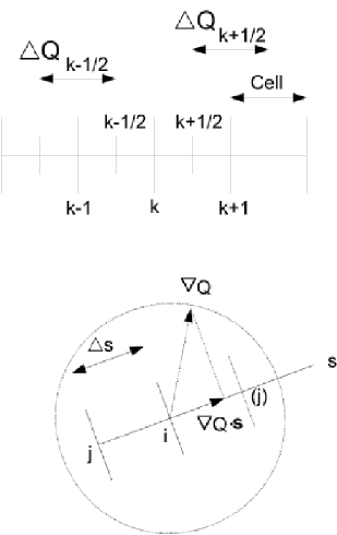
Figure 1: Cartoon illustration of how the gradient of a thermodynamical quantity $Q$ is computed for the purpose of implementing the limiter introduced by van Leer (1979). The upper figure describes the standard case of the computation in case the variable $Q$ is assigned on a regular grid. The lower figure is for the case, relevant for our implementation of GSPH, in which the variable $Q$ is assigned at the positions of the $i$-th and $j$-th particles.

In higher-order (i.e. second-order and above) schemes, thermodynamical quantities must be limited to obtain a stable description of the discontinuity. This is obtained by implementing a limiter, which is defined as “a non-linear algorithm that reduces the high-derivative content of a subgrid interpolant in order to make it non-oscillatory” (van Leer, 2006). For instance, Inutsuka (2002) imposed that a second-order reconstruction is performed when the components of velocity gradients, at the position of the two particles, parallel to the $s$-axis have the same sign, while one resorts to a first–order reconstruction in case of discordant signs.

We note that Godunov (1959) proved a theorem which states that any advection scheme preserving the monotonicity of the solution is at most first-order accurate. This holds only if the discretization of the advection equation is linear. Thus, non-linear schemes are needed to achieve higher order accuracy. On the other hand, for them to be useful, higher-order schemes need to include in the interpolator a prescription to limit spurious oscillations. For example, in the context of Eulerian schemes, Van Leer (1979) proposed to employ a “harmonic gradient averaging” technique, in which the gradient of the thermodynamical quantity $Q$ is the harmonic average of the gradients in the $k+1/2$ and $k+3/2$ cells, namely:

$$\Delta Q_{k+1/2}={{2\Delta_{k}Q\Delta_{k+1}Q}\over{\Delta_{k}Q+\Delta_{k+1}Q}}\,,$$ (18)

where $\Delta_{k}Q=Q_{k+1/2}-Q_{k-1/2}$ and we assumed unity value for the cell size. In this notation, $Q_{k+1/2}$ indicates the mass-averaged value of a given thermodynamical variable in the cell $k+1/2$, having boundaries at $k$ and $k+1$, thus with the obvious extension for the meaning of $Q_{k-1/2}$. The mass-averaged gradients of the variable $Q$ at half-cell positions, $\Delta Q_{k\pm 1/2}$, are then used to estimate the right-state and left-state values of $Q$ at the interface:

$$\begin{array}[]{lcl}\vspace{5mm}Q_{L,R}\!=\!\!\left\{\!\begin{array}[]{l}\vspace{5mm}Q_{k\pm 1/2}\mp\Delta Q_{k\pm 1/2}/2\;\;\mbox{\rm if }\Delta Q_{k-1/2}\Delta Q_{k+1/2}>0,\\ Q_{k\pm 1/2}\;\;\mbox{\rm if }\Delta Q_{k-1/2}\Delta Q_{k+1/2}<0,\end{array}\right.\end{array}$$ (19)

It can be shown (van Leer, 2006) that such an interpolator corresponds to a standard central difference of the quantities $Q$, limited by a term of order $(\Delta s)^{2}$ which depends on the rate of change of the quantity itself through its second-order derivative. Thus, the harmonic gradient averaging is a good example of a non linear interpolator with a built-in limiter.

In the case of an Eulerian scheme implemented on a regular Cartesian grid, Eq. 18 uses three adjacent cells, namely $k-1/2$, $k+1/2$ and $k+3/2$. Clearly, this prescription to compute gradients can not be directly generalised to our GSPH scheme, where the values of the variable $Q$ are assigned at the positions of the $i$-th and $j$-th particles, while there is no a third particle to form a regular grid along the direction of the separation vector ${\bf x}_{i}-{\bf x}_{j}$.

In the upper part of Figure 1 we schematically show how quantities are evaluated in the Eulerian scheme, while the lower part shows our extension of the implementation of the van Leer (1979) limiter in the case of the unstructured grid, which is relevant for the GSPH. In this case, we only have quantities $Q_{i}$ and $Q_{j}$ evaluated at the particles positions. We define the equivalent of the Eulerian $\Delta Q_{k-1/2}$ as:

$$\Delta Q_{1}={{Q_{j}-Q_{i}}\over{\Delta s}}\,,$$ (20)

where $\Delta s$ it the distance between the two particles. To evaluate the equivalent of $\Delta Q_{k+1/2}$, we use a “ghost” particle $(j)$, which is located the same distance $\Delta s$ from the $i$-th particle, but in the opposite direction along the $s$ axis. Since we have the SPH estimate of the gradient $(\nabla Q)_{i}$ at the position of the $i$-th particle, we can compute the expected value $Q_{(j)}$ at the position of the “ghost” particle as

$$Q_{(j)}=Q_{i}+(\nabla Q)_{i}\cdot{\bf s}\Delta s\,.$$ (21)

Thus, the equivalent of the quantity $\Delta Q_{k+1/2}$, that we defined in the case of the regular grid, is

$$\Delta Q_{2}={Q_{i}+(\nabla Q)_{i}\cdot{\bf s}\cdot\Delta s-Q_{i}\over\Delta s}=\nabla Q\cdot{\bf s}$$ (22)

Therefore, $\Delta Q_{2}$ is simply the projection of the gradient of the quantity $Q$ on the $s$-axis, In general, it is $\Delta Q_{1}\neq\Delta Q_{2}$, since $Q_{2}$ depends on the 3D properties of the field $Q$ through its gradient computed at the $i$-th particle, while the latter only depends on the values of the field at the positions of the $i$-th and $j$-th particles. Of course, the same calculation can be repeated for the $j$-th particle using a “ghost” particle $(i)$, which is defined in the same way. Therefore, the extension of Eq.(18) to the case of an unstructured grid, defined by particle positions, reads

$$\begin{array}[]{lcl}\vspace{5mm}{{\partial Q}\over{\partial s}}\!=\!\!\left\{\!\begin{array}[]{l}\vspace{5mm}{{2\Delta Q_{1}\Delta Q_{2}}\over{\Delta Q_{1}+\Delta Q_{2}}}\;\;\mbox{\rm if }\Delta Q_{1}\Delta Q_{2}>0,\\ 0\;\;\mbox{\rm if }\Delta Q_{1}\Delta Q_{2}<0,\end{array}\right.\end{array}$$ (23)

Having computed the values of the gradients ${{\partial Q}\over{\partial s}}$ at the positions of the $i$-th and $j$-th particles, we can assign the values of thermodynamical quantities on the left and right states at the interface, following the same procedure as in I02. We will refer to this implementation as “second order reconstruction with van Leer limiter” (see van Leer, 2006, for a detailed description) .

Once we have thermodynamical variables assigned on the left and right states ($P_{R,L}$, $v_{R,L}$, $\rho_{R,L}$), we still have to solve the RP. Many Riemann solvers do exist in the literature (e.g. Toro, 1999, and references therein). Here, we use the iterative solver originally proposed by (van Leer, 1979) and described in detail by Cha & Whitworth (2003). We refer to this paper for a complete description of the implementation of this solver. The general idea is (i) to define the Lagrangian shock speed $W$ starting from an initial guess based on the values of $P_{*}$ and $v_{*}$; (ii) calculate the values of the tangential slopes $Z={dP_{*}\over dv_{*}}$; (iii) use these slopes to evaluate the new values of $P_{*}$ and $v_{*}$; (iv) iterate until the variation in $P_{*}$ with respect to the previous iteration falls below a given threshold value, namely, is less than 1.5 %. We also checked that using a different solver, namely a Newton iterative solver (e.g. van Leer, 2006), the results of our hydrodynamical tests do not appreciably change. Both the Van Leer and the Newton solvers are exact. Usually, they provide a converged result in 5-7 iterations. A significant speed-up of the code could be obtained by using instead an approximate one-iteration solver, such as the Harten–Lax–van Leer–Contact (HLLC) solver proposed by (Toro et al., 1994).

In summary, the implementation of the Godunov method in our GSPH version of the GADGET-3 code requires the following steps.

1.

Estimates of the volume function $V(s)$ and of the position $s_{*}$ of the interface between each pair of particles. In our implementation, this can be done through either a linear interpolation or a cubic spline;

2.

Choice of the spatial order of the reconstruction of the thermodynamical values at the interface position. Currently, we have implemented first and second order reconstructions. A third order scheme, such as the Piece-wise Parabolic Method (PPM), could in principle be implemented.

3.

Choice of the limiter, in the case of second-order reconstruction. We have implemented both the “standard” reconstruction, as in Inutsuka (2002), and the reconstruction scheme proposed by van Leer (2006).

4.

Choice of the solver for the RP. We have implemented two equivalent exact solvers, namely the iterative solver proposed by van Leer (1979) and the Newton solver. We will present results based on the former solver, while we have verified that identical results are obtained by using the Newton solver.

We provide in Table 1 a description of the variants of the hydrodynamical schemes that we compare through the tests described in the following section.

The first one is the original GADGET-3 entropy conserving scheme, tagged GADGET. We then use a traditional, energy conserving SPH scheme (TradSPH). In this case, however, we use a Gaussian kernel, rather than the B–spline one implemented in GADGET. We tag as GSPH our new reference implementation, which uses cubic spline interpolation for volumes, second-order reconstruction of thermodynamical variables at the interface, with the limiter and the iterative solver for the Riemann problem, both proposed by van Leer (1979). Furthermore, we tag as GSPH-I02 the version based instead on using the limiter adopted in I02, with GSPH-1ord the version based on a first-order reconstruction of the thermodynamical quantities at the RP interface, and with GSPH-VLin the version based on the linear interpolation for the volume function $V(s)$ (see Appendix). Finally, we also implemented the version of the Godunov SPH scheme (Cha & Whitworth, 2003), which is described by Eqs.(16) and (17), rather than by actual equations of GSPH involving the volume integrals, as in Eqs.(5) and (8). We will refer to this scheme as GSPH-CW.

Name	Hydrodynamic scheme	Implementation details	Sod	KH	Blob
GADGET	SPH	Entropy conserving with B-spline kernel.	100	442	50
TradSPH	SPH	Energy conserving with Gaussian kernel.	100	–	–
GSPH	GSPH	Based on Eqs. (16) and (17) with cubic spline for volume interpolation,	100	100 & 300	200
		second-order reconstruction and limiter by van Leer (1979).
GSPH-I02	GSPH	The same as GSPH but based on the limiter by Inutsuka (2002).	100	100 & 300	200
GSPH-1ord	GSPH	The same as GSPH-I02 but using the first–order reconstruction	100	300	200
		for the RP solution.
GSPH-VLin	GSPH	The same as GSPH, but using the linear interpolation for the volume		300	200
		function $V(s)$, as in Eq. (25).
GSPH-CW	GSPH	Same as GSPH  but based on Eqs. (16) and (17) by Cha & Whitworth (2003).	100	–	200

Table 1: Characteristics of the hydrodynamical schemes implemented and of the hydrodynamic tests carried out. Column 1: name of each scheme; Column 2: hydrodynamic method on which each scheme is based; Column 3: basic description of the implementation details of each scheme (see Section 3 for further details); Columns 4, 5 and 6: number of neighbour used for each scheme in the Sod shock tube, Kelvin–Helmholtz and blob test, respectively.

4 Results

We describe in this section the tests of our GSPH implementation in the GADGET code. The hydrodynamic tests performed are the shock tube, the development of Kelvin–Helmholtz instabilities in a shear flow and the disruption of a cold dense blob moving in a hot wind.

4.1 Shock tube

We first consider the standard Sod shock-tube test (Sod, 1978), which provides a mean to validate the code capability to describe basic hydrodynamic features. Initial conditions are the same used by Springel (2005) to test the GADGET SPH scheme. An ideal gas with politropic index $\gamma=1.4$ is considered initially at rest, filling half space with gas at unit pressure and density ($\rho_{1}=1$, $P_{1}=1$), and the other half space with lower density ($\rho_{2}=0.25$) and lower pressure ($P_{2}=0.1795$) gas. Despite the intrinsic one-dimensional nature of the test, initial conditions are generated in three dimensions with an irregular glass-like distribution of equal-mass gas particles. A periodic box was chosen having a longer size in the $x$-direction, with $(L_{x},L_{y},L_{z})=(60,1,1)$. A total number of 75000 particles have been included in the initial conditions. We run this test with four different hydrodynamic schemes (see Table 1), namely GADGET, TradSPH, GSPH, GSPH-CW and GSPH-I02. In all cases, the test has been run by using 100 neighbours within the kernel.

We show our results for the SOD test by restricting the range of $x$ coordinates to vary between 20 and 40. In fact, since we use periodic initial conditions, we have two shocks inside the computational domain. We only focus on one of them, while discarding the uninteresting unperturbed regions [0:20] and [40:50] along the $x$-axis. Results for this test are shows as scatter plots of density, pressure, velocity and entropy, all expressed in internal code units. In fact, performing a binning often smooths out details which are useful to understand the differences in the behaviours of our the different hydrodynamic schemes.

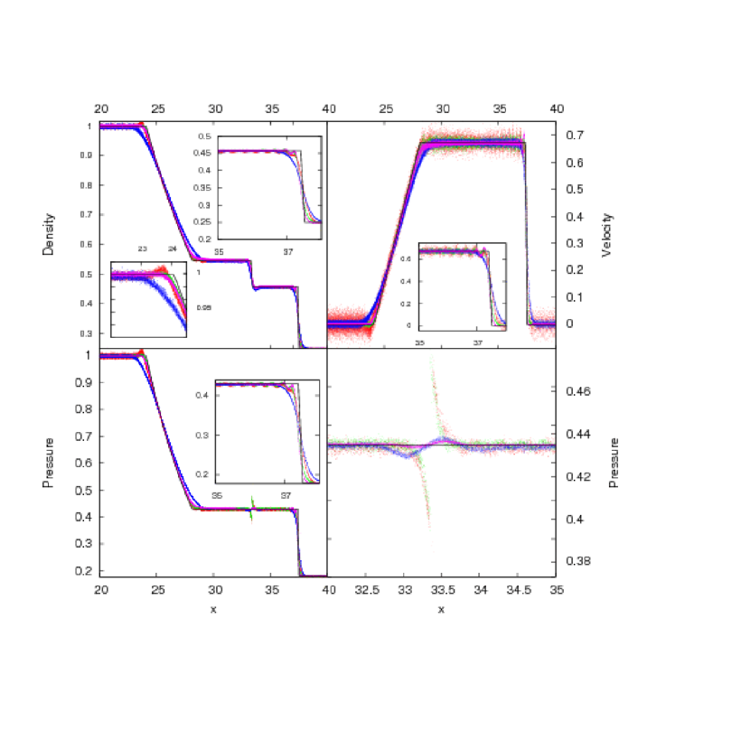
Figure 2: Comparison between the results of different hydrodynamic schemes for the Sod shock tube. Scatter plots of the particle density, velocity and pressure are shown in the upper left, upper right and bottom left panels, respectively. The bottom right panel shows a zoom of the pressure around the contact discontinuity. Red points are for the entropy–conserving GADGET formulation, green points for the TradSPH formulation, blue points for the GSPH-CW formulation and magenta points for our reference GSPH formulation (see Table 1). In each panel, the black continuous line indicates the exact solution. The insets emphasise the different behaviour of the four schemes, as also discussed in the text.

We show in Figure 2 density, pressure, and velocity at the time $T=5$, when the shock is well developed, for the GADGET, TradSPH, GSPH and GSPH-CW schemes (red, green, blue and magenta points, respectively).

A well known problem of SPH codes in solving the Sod shock tube is the appearance of a pressure discontinuity (“pressure blip”) at the position of the contact discontinuity. This is at variance with respect to the exact analytic solution, that predict instead pressure to be continuous across this discontinuity. This pressure discontinuity arises as a consequence of the error that the SPH scheme makes in correctly estimating the density gradient at the density discontinuity. As a result, a sort of spurious surface tension force arises, due to the opposite signs that the pressure gradients have on the two sides of the discontinuity. In fact, GADGET and TradSPH formulations clearly show a pressure blip at $x\approx 33.5$, where the discontinuity is located. This is emphasised in the bottom left panel of Fig. 2, which provides a zoom of the pressure in this region. Since this spurious pressure feature arises from errors in the computation of density at the discontinuity, its origin can be traced back to the incorrect estimate of the $1/\rho$ SPH volume associate to each particle. Two conceptually different solutions to this problem can be then devised. A first one is based on improving the density estimate in the computation of density gradients across the discontinuity (e.g. Read et al., 2010). A second one relies instead on the introduction of thermal diffusion across the discontinuity, which masquerade the effect of the error in the volume estimate and prevents the onset of the surface tension there (e.g. Price, 2008).

Cha & Whitworth (2003) noticed that the GSPH-CW scheme was in fact able to prevent the development of the density blip. Since this scheme does not pay attention to correctly estimate volumes, its behaviour should be ascribed to the inclusion of a diffusion term. This term is indeed provided by the $\left[{\bf v}^{*}-{\bf x}_{i}^{*}\right]$ appearing on the r.h.s. of Eq.(16), which in fact described a net exchange of thermal energy, with a zero total mass exchange, between each particle pair. Its effect is similar to that of adding an artificial thermal diffusion term in the energy equation. The main difference, however, is that here such a mixing term naturally arises from the Godunov scheme.

As shown in the bottom–right panel of Fig. 2, we do confirm that this scheme does not produce a pressure discontinuity, which is replaced by an oscillation around the exact solution. Therefore, while diffusion prevents the ”pressure blip”, inaccuracy in the density estimate is still present and induces the appearance of a spurious, although much reduced, pressure force at the contact discontinuity. Quite interestingly, this spurious force is further, and greatly, reduced in our reference GSPH scheme. In this case, second–order accuracy in density estimate is enforced through the computation of the convolution integrals in Eqs. (5) and (8) (see also I02). The net effect is a significant improvement in the behaviour of pressure across the discontinuity.

To further emphasise the different behaviour of the SPH-based (GADGET and TradSPH) and GSPH-based (GSPH and GSPH-CW) schemes, we plot in Figure 3 the fractional variation of the entropy of particles as a function of their final position, across the discontinuity. Quite clearly, entropy variation is only determined by the presence of weak shocks for the GADGET and TradSPH scheme and, therefore, can only have positive sign. On the other hand, the presence of diffusion in the GSPH and GSPH-CW allows an exchange of internal energy across the discontinuity. This diffusion manifests itself with both positive and negative variations of entropy, with lower-density particles located on the right side of the discontinuity loosing thermal energy in favour of particles located on the other side of the discontinuity. It is such a mixing that is responsible of the damping of the pressure blip.

Both GADGET and TradSPH schemes show pressure wiggles immediately before the shock wave, which is located at $35<x<37$ (see the inset in the pressure panel in Fig. 2). Such wiggles in pressure correspond to wiggles in the velocity, as shown in the top-right panel of Fig.2 at the same position. Note that velocity wiggles are largest for GADGET and smallest for GSPH. Wiggles are also present in the GADGET run at the same position for the density variable (upper-left panel). The insets in the two panels show a blow-up of the region around the shock wave positions, and emphasise the presence of such wiggles. The prominence of the pressure wiggles in the GADGET simulation is due to the lack of thermal energy diffusion that characterises this hydrodynamic scheme. In a sense, these wiggles have the same origin as the wiggles in velocity appearing in the shock-tube test when artificial viscosity is not included (e.g., Rosswog, 2009). In fact, artificial viscosity removes velocity wiggles since it effectively provides a diffusion of momentum at the shocks. In a similar way, diffusion of thermal energy associated to the GSPH scheme is effective in removing wiggles in pressure at such discontinuities.

In the upper-right panel of Figure 2, we also notice that the scatter in the velocities is minimum for GSPH and maximum for GADGET. The shock wave is better captured by GADGET and GSPH, with GSPH-CW performing worse. It is quite remarkable that GSPH is able to correctly capture the shock, while preventing at the same time the appearance of noise in the velocity field, without the introduction of an artificial viscosity term in the momentum equation. Furthermore, the better accuracy of GSPH with respect to GSPH-CW is the consequence of the improved accuracy of the former scheme.

The shape of the rarefaction fan in density and pressure (upper and lower left panels in Fig. 1, respectively) are better captured by GADGET and TradSPH formulations, while GSPH-CW shows a much smoother behaviour. GSPH also shows a slight smoothing of density and pressure at the beginning and at the end of the rarefaction fan. On the other hand, GADGET produces a piling-up of particles at the onset of the fan, corresponding to an excess of particles having low velocities, at the same position. This feature can be better appreciated in the lower inset of upper-left panel of Fig. 1.

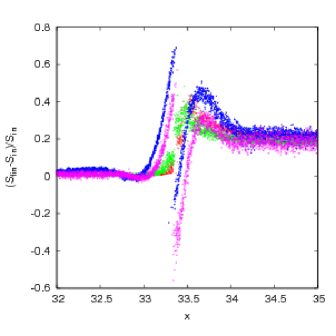
Figure 3: Entropy variation in GADGET, TradSPH, GSPH and GSPH-CW hydrodynamic scheme for the Sod shock test around the contact discontinuity. Colour coding is the same as in Figure 2. Here we show the difference between the final and initial entropy of particles, normalised to their initial entropy, as a function of final particle positions.

Figure 4 shows results for the Sod test, when we use different implementation for the GSPH formulation. Besides our standard implementation of GSPH, we also show results based on the limiter used by I02 in its implementation of GSPH (GSPH-I02) and on the first–order reconstruction at the interface $s_{*}$ for the solution of the RP (GSPH-1ord; see Table1). From the behaviour of density and pressure, it is clear that a first-order reconstruction results in a more diffusive behaviour: the shape of the rarefaction ramp and of the velocity profile at the position of the shock wave are smoother than for the other two implementations. For the same reason, no velocity wiggles appears when this formulation is used. The difference between the two limiters is instead clear when we analyse the density right before the rarefaction fan. There, the standard limiter produces an accumulation of particles, similar to what we found when using the SPH GADGET formulation. Such an accumulation is instead eliminated by adopting the limiter by van Leer (1979). Furthermore, the use of this limiter avoids the accumulation of low-velocity particles after the position of the shock wave, as can be seen in the upper-right panel. The pressure blip at the density discontinuity is erased in all of these three schemes, thus we do not show a zoom-in for the pressure.

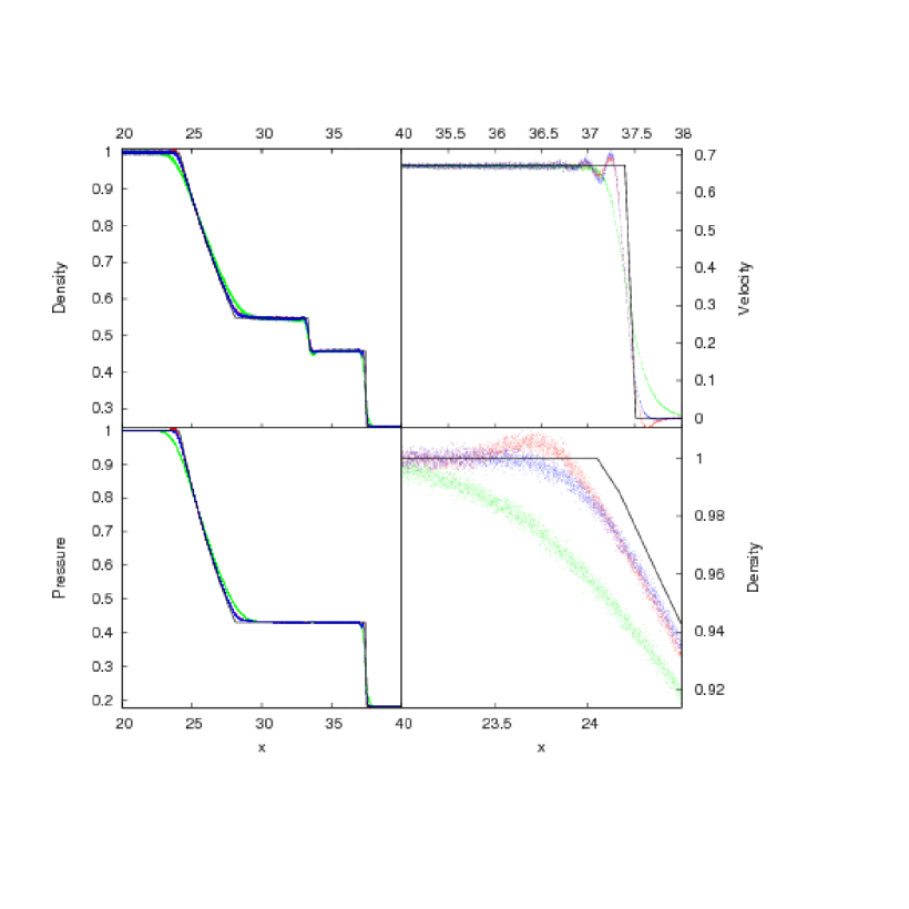
Figure 4: Comparison between the results of different implementations of the GSPH Equations (5) and (8) for the Sod shock tube. Scatter plots of particle density, velocity and pressure are shown in the upper left, upper right and bottom panels, respectively. The bottom-right panel shows a zoom-in of pressure behaviour around the onset of the rarefaction fan. Red points are for the GSPH with the standard limiter of Inutsuka (2002) (GSPH-I02), green points for the same scheme when using a first-order reconstruction of density and pressure at the interface in the solution of the Riemann problem (GSPH-1ord), while the blue points correspond to our standard implementation (GSPH) based on using the limiter by van Leer (1997) and the third-order spline interpolation of volumes.

4.2 Kelvin-Helmholtz instability

The Kelvin-Helmholtz instability occurs across a contact discontinuity in the presence of a tangential shear flow. It belongs to a class of tests that have been used over the last few years to assess the capability of SPH and grid-based methods to capture fluidodynamical instabilities (e.g. Agertz et al., 2007; Price, 2008; Wadsley et al., 2008; Read et al., 2010; Valcke et al., 2010). It describes the evolution of two fluids having different densities and in pressure equilibrium, moving with opposing velocities. The interface between the fluids is perturbed leading to a phase in which fluid layers develop vortex instabilities, with subsequent mixing of the two phases (Chandrasekhar, 1961). We remind here that a two–dimensional version of this test has been also recently discussed in detail by Cha et al. (2010) to assess the capability of GSPH to describe instabilities. We extend here this test in three-dimensions for our GADGET implementation of GSPH.

The KH test that we present here belongs to the “Wengen” suite of hydrodynamical tests, and is described in detail by Read et al. (2010). An ideal idea gas with politropic index $\gamma=1.4$ and mean molecular weight $\mu=1$ is assumed. Initial conditions are generated in the periodic simulation domain $(L_{x},L_{y},L_{z})=(256,256,16)$ kpc centered on the origin. Two domains with $|y|<64$ kpc and $|y|>64$ kpc corresponds to the two fluids having $\rho_{1}=2\rho_{2}$, $T_{1}=0.5T_{2}$ and opposing velocities with the same modulus $v$. In this test, $\rho_{2}=3.13\cdot 10^{-8}$ M_⊙ kpc^-3, $T_{2}=3\cdot 10{{}^{6}}$K, and $v=40$ km s^-1. Equal-mass gas particles are initially located on a grid, whose spacing in the two domains is set in such a way to reproduce the difference in density. Instabilities are triggered by imposing a velocity perturbation along the $y$-direction, having a characteristic wavelength $\lambda=128$ kpc. The characteristic KH time-scale for the development of instabilities from this perturbation is

$$\tau_{KH}={\lambda(\rho_{1}+\rho_{2})\over 2v(\rho_{1}\rho_{2})^{1/2}}\,.$$ (24)

The units used in the Wengen tests are: kpc for length, km s^-1 for velocities, and $10^{10}$ M_⊙ for masses. In this system, the unit of time is $t_{*}=0.977$ Gyr. Using the perturbation described above, $\tau_{KH}\simeq 3.32$ Gyr. Initial conditions have been generated using 774.144 gas particles. We carried out this test using different implementations of the GSPH scheme: our reference scheme (GSPH), the scheme based on the limiter adopted by I02 (GSPH-I02), the scheme based on a first-order reconstruction for the thermodynamical quantities at the interface (GSPH-1ord), and the scheme based on the linear interpolation of the volume function $V(s)$ (GSPH-VLin). In order to reproduce the results reported for the GADGET code on the web site of the Wengen tests, we carried out the KH test in this case using 442 neighbours. As for the different implementations of the GSPH scheme, we always used 300 neighbours within the Gaussian kernel, while we also checked the effect of using instead 100 neighbours for the reference GSPH scheme and for the GSPH-I02 scheme.

We show in Figure 5 the development of the KH instability for GADGET, GSPH and GSPH-I02at three different times, namely $0.5\tau_{KH}$,$\tau_{KH}$ and $2\tau_{KH}$. It is clear that, while the standard entropy-conserving SPH scheme dumps the instability, both our GSPH and GSPH-I02 schemes successfully capture its development. At $t=\tau_{KH}$, vortexes begin to show up, and at $t=2\tau_{K}H$ they are fully developed and display the typical “cat-eye” structures in gas density.

This figure confirms the results reported by Cha et al. (2010) and demonstrates the capability of the GSPH scheme to develop gas–dynamical instabilities. Note that, while the damping of the instability in the GADGET entropy conserving scheme is due to the use of an artificial viscosity and to development of a “artificial surface tension” force at the interface, originated by the repulsion of SPH particle at the discontinuity (see e.g Price (2008); Cha et al. (2010)), the former is absent and the latter strongly reduced in GSPH schemes (see Inutsuka (2002); Cha et al. (2010) for a discussion of the different estimate of density on GSPH and on its effect on the artificial surface tension). The much improved description that the Godunov SPH scheme provides in describing the development of KH instabilities has to be ascribed to the fact that this method is based on explicitly computing the convolution integrals in Eqs. (5) and (8), to a $O(h^{2})$ accuracy, through the interpolation of the volume function $V(s)$.

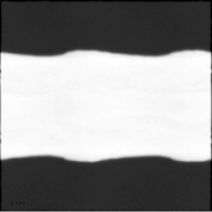
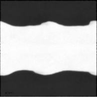
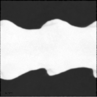
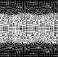
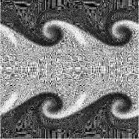
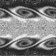
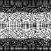
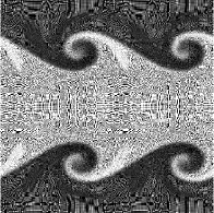
Figure 5: Development of the Kelvin-Helmholtz instabilities at different times, as described by the GADGET (upper panels), GSPH-I02 (central panels) and GSPH (bottom panels) scheme. Results are shown at three different times, $0.5\tau_{KH}$,$\tau_{KH}$ and $2\tau_{KH}$ in the left, middle and right panels, respectively. Each panel report the the projected density for a slice of coordinates $-3.5<z<5.5$ kpc. Colour scale is linear and ranges from $2\times 10^{-7}M_{\odot}$kpc^-2 (black) to $5\times 10^{-7}M_{\odot}$kpc^-2 (white).

Figure 6 shows a blow-up of one of the curl structures, which forms after the KH instability is fully developed, for both the GSPH and the GSPH-I02 schemes. The difference is small, but the Van Leer limiter is able to more neatly capture the vortex structure. We hypotize that the reason for this behaviour is that the Van Leer limiter is capable to slightly reduce the intrinsic residual numerical diffusion associated to the Riemann solver, with respect to the limiter implemented by I02.

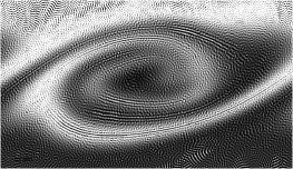
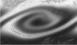
Figure 6: Blow-up of the curl structure developed by the KH instability at $t=6.75$, for GSPH (left panel) and by GSPH-I02 (right panel). The structure shown here developed in the ranges of coordinates $78<x<210$ kpc and $161<y<237$ kpc. We show the projected density for a slice of coordinates $-3.5<z<5.5$ kpc. Colour scale is linear and ranges from $2\times 10^{-7}M_{\odot}$kpc^-2 (black) to $5\times 10^{-7}M_{\odot}$kpc^-2 (white).

To further highlight the different ways in which entropy–conserving SPH and GSPH respond to the velocity perturbation across the contact discontinuity in the KH test, we show in Figure 7 a scatter plot of the pressure of gas particles as a function of the $y$ coordinate (i.e. in the direction parallel to the direction to the velocity perturbation triggering the KH instability). This scatter plot includes only the particles contained within the same vortex region shown in Fig. 6. It is clear that GADGET develops a pressure “blip” at the discontinuity, similarly to what happens in the shock tube test. On the contrary, the blip basically disappeared in the GSPH scheme, and a complex pressure structure, associated to the vortex, develops.

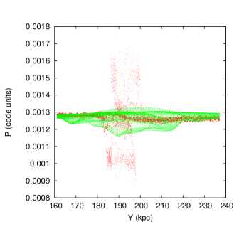
Figure 7: Pressure of gas particles as a function of their $y$ coordinates for GADGET (red dots) and GSPH (green dots), at time $t=2\tau_{KH}$, in correspondence of the same vortex shown in Fig. 6, $78<x<210$ kpc, $161<y<237$ kpc, $-3.5<z<5.5$ kpc.

In order to further highlight the role that different details in the implementation of the GSPH scheme have in the development of the KH instability, we also studied the effect of varying the number of neighbours, the reconstruction prescription and the volume estimates. The results of these tests are shown in Figure 8. The most striking effect is given by the reconstruction order for the thermodynamical quantities at the interface where we solve the Riemann problem. A first-order reconstruction (GSPH-1ord; upper right panel) is so diffusive that the KH instability does not develop at all. This demonstrates how crucial it is for the development of the KH instability to choose a scheme that gives the lowest possible degree of diffusion where it is not required. In fact, the GSPH-1ord has been shown to be effective in preventing the formation of the pressure blip in the shock tube test (see Fig.2). However, the excess of diffusion, which manifests itself in the shock tube test as a smooth transition at the rarefaction fan, is such to prevent the development of the KH instability. We also note that it is quite important to use a rather large number of neighbours: decreasing its number from 300 to 100 (upper central panel) produces a smoother structure of the vortexes, and fails to capture their “cat-eye” shape. This is due to the increase of noise in the density estimate at the discontinuity, that arises when a smaller number of neighbours is used. On the other hand, the KH test is also sensitive to the precision of interpolation of the volume function: using a linear interpolation of this function (GSPH-1ord; lower central panel), develops instabilities whose “curl” structure is however less resolved than for a cubic interpolation. As for the GSPH-CWscheme, based on Eqs. (16) and (17), the large amount of diffusivity is such to prevent the development of KH instabilities. The lack of accuracy of this scheme is due to two main differences with respect to our reference GSPH scheme: firstly, Eqs. (16) and (17) are not derived from the convolution of the equation of motion and energy conservation; secondly, in this scheme we have no means to locate the position of the interface for the solution of the RP, thus implying that we are effectively resorting to a first-order reconstruction.

As a further check, we run another KH test, in which we multiplied the y-axis velocity perturbation by a factor of five. The aim of this test is to verify whether lower-order schemes succeed in following the development of the KH instability when the perturbation is strong enough. We show the results of this test in Figure 9, at the time $t=\tau_{KH}$ of our “standard” test, so that also the amplification of the perturbation is appreciable. In this case, the entropy conserving GADGET scheme develops arms, but fails to capture the development of the vortexes. On the other hand, GSPH is confirmed to successfully capture the instability, while the GSPH-1ord and GSPH-CW schemes confirm to be very diffusive and to smooth out the instability. The results of this test demonstrate that a higher-order GSPH scheme is necessary to correctly treat the development of KH instabilities.

In summary, the results shown in this Section confirm and extend the 2D test results presented by Cha et al. (2010) on the capability of GSPH to follow the development of KH instabilities. We demonstrated that the performance of GSPH is further improved by adopting the limiter by van Leer (1979), instead of that of I02, used by Cha et al. (2010). Furthermore, our results also highlight that the development of the instability is inhibited in different ways by (a) errors in density estimate at the discontinuity, as in standard SPH or when using a small number of neighbours in GSPH, and (b) numerical diffusion, which increases when using a less accurate first-order reconstruction of thermodynamical variables at the interface.

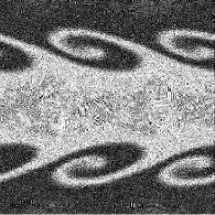
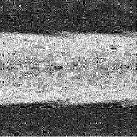
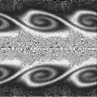
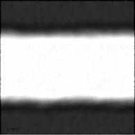
Figure 8: Effect of different GSPH implementations on the KH instability at $t=2\tau_{KH}$. Results are shown for our reference GSPH scheme using 300 neighbours (upper left panel) and 100 neighbours (upper central panel), using GSPH-1ord with first-order reconstruction at the interface (upper right panel), and using GSPH-I02 with the limited by I02 (bottom left panel), using GSPH-VLin with linear interpolation for the volume function (bottom central panel), and for the GSPH-CW scheme based on Eqs. (17) and (16) (bottom right panel). Ranges of coordinates and gray-scale density coding are the same as in Fig. 5.

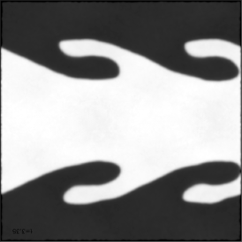
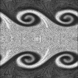
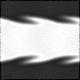
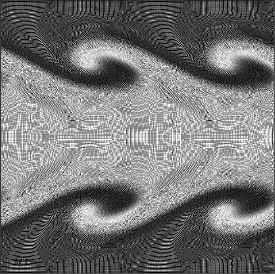
Figure 9: KH test with a stronger velocity perturbation on the y axis. We show the result at the time $\tau_{KH}=1$ of our standard KH test. Results are shown for the entropy conserving GADGET scheme (upper right panel), for our reference one GSPH (upper left panel), for GSPH-CW (lower left panel) and for GSPH-1ord (lower right panel). Ranges of coordinates and gray-scale density coding are the same as in Fig. 5.

4.3 The blob test

This test describes the disruption of a cold gas cloud having uniform density, moving in pressure equilibrium against a hot lower-density wind. This test has been used by Agertz et al. (2007) to assess the capability of different hydrodynamic schemes to describe the blob disruption due to the onset of KH and Rayleigh–Taylor instabilities (see also Read et al., 2010). Cha et al. (2010) recently used a two–dimensional version of this test to assess the performance of their GSPH implementation. The version of the blob test that we use here also belongs to the “Wengen” suite. A full description of the initial conditions is provided by Read et al. (2010). The simulation domain is given by a periodic rectangular box with $(L_{x},L_{y},L_{z})=(2,2,8)$ Mpc, with the origin of the coordinates located at the centre of this domain and the blob initially located at $(0,0,-3)$ Mpc. The radius of the cloud is set to $r_{c}=197$ kpc. Internal density of the cloud is a factor $\chi=10$ higher that in the external medium, with the temperature being correspondingly a factor 10 lower so as to fulfil the condition of pressure equilibrium. Initial conditions are generated by placing equal-mass particles in a lattice configuration, so as to satisfy the above density requirements. The velocity of the wind is $v=1000\,\,{\rm km\,s^{-1}}$. An initial instability is also used to the surface layer of the cloud to trigger a large-scale instability (see Read et al., 2010, for a full description of the initial conditions). Units of measure for length, velocity, mass and time are the same as in the KH test. Initial conditions are generated using $10^{7}$ gas particles. We use 200 neighbours for the test based on the different implementations of GSPH, and 50 for GADGET, which uses the B–spline kernel (see Table 1). Following Agertz et al. (2007), we define the cloud crushing time, $\tau_{cc}={r_{c}\sqrt{\chi}\over v}=0.61$ Gyr, which gives the typical time–scale for the evolution of the cloud moving at supersonic velocity.

The results of this test have implications for a number of relevant astrophysical and cosmological applications, in which a dense gas cloud interact with a lower density medium. For instance, this is the case of a cold molecular cloud in the inter-stellar medium, which interacts with ejecta from a nearby exploding supernova. Another example is provided in cosmological simulations by substructures bringing relatively cold gas which merge into larger halos permeated by hotter gas during the hierarchical assembly of galaxy groups and clusters.

The blob is expected to be initially destabilised by Richtmyer-Meshkov instability (RM) and by Rayleigh–Taylor (RT) instability and subsequently further dissolved by KH instability. We show in Figure 11 the evolution of the projected gas density in this test at three different times, for the GADGET (upper panels), GSPH (bottom panels) and GSPH-I02 (middle panels) hydrodynamical schemes. As expected, the limitations of the standard entropy conserving formulation of SPH in following hydrodynamical instabilities make this scheme unable to describe the disruption of the cold blob (see Agertz et al., 2007, for a detailed discussion). Already at early times, $t=4$ (left panels), the GADGET simulation develops less hydrodynamical instabilities in the up-wind part of the blob.

Even if the total number of gas particles in our blob simulation is fairly high, force resolution, which is directly related to the mean interparticle separation, is lower than in the KH simulations. In fact, the mean interparticle separation is $14.7$ kpc for the blob test, and $0.89$ kpc for the KH test. For this reason, the development of hydrodynamical instabilities is not clearly visible in Figure 11. In order to show the different behaviour of the different numerical schemes, we show in Figure 10 the velocity field in a thin slice, centred on the blob, at the time $t=4$ when such instabilities begin to develop. The upper-left panel shows the field for GADGET, the upper-right one for GSPH , the lower-left panel for GSPH-CW and the lower-right one for GSPH-1ord. Velocities are computed with respect to the rest-frame of the blob.

   

   

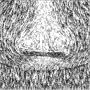
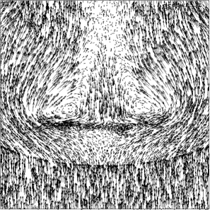
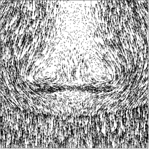
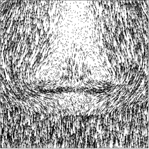
Figure 10: Velocity field, at the time $t=4$, for the “blob” test, in the region surrounding the blob itself. We plot a slice near the center of the blob, with $900<x<100$ kpc, $400<y<1600$ kpc and $1500<z<3500$ kpc. We show the velocity field for GADGET(upper-left panel), GSPH(upper-right panel), GSPH-CW (lower-left panel) and GSPH-1ord (lower-right panel). Each arrow shows the velocity of one gas particle; we undersampled the simulation by a factor 0.0025, for clarity. Velocities are computed in rest frame of the blob.

The difference between GADGET and GSPH is striking. Hydrodynamical instabilities create vortexes in the back of the blob in both cases. Quite clearly, the GSPH scheme is by far most effective in resolving these vortexes and creating a downstream velocity flux. Also, the disruption of the blob front due to RT instabilities is marginally apparent in this figure. Note that the GSPH-CW scheme is also more effective than GADGET in capturing the vortex structures. This is due to the absence of an artificial viscosity in such a scheme, which prevents the development of of vortex structure in the velocity field. However, the large diffusivity of GSPH-CW causes the suppression of the downstream flux. Finally, the behaviour of the GSPH-1ord scheme is intermediate between the other two GSPH schemes, since it is more diffusive than standard GSPH but less so than GSPH-CW .

The difference of the GADGET evolution with respect to the two GSPH implementations shown in Fig. 11 is even more apparent at $t=6$. At this time the RT and RM instabilities appearing in the GPSH simulations are further dissolved into filamentary and curl-like structures, which are produced by the onset of KH instabilities. At $t=8$ (right panels) the bulk of the gas initially contained in the cold blob still forms a compact structure in the GADGET simulation. On the contrary, in both GSPH simulations the blob is basically dissolved at this time. The result for the GSPH-I02 case are fully consistent with the two–dimensional blob test presented by Cha et al. (2010), who also used the I02 limiter.

A comparison between the results obtained from the I02 and the van Leer (1979) limiters show that they perform quite similarly in this test. This suggests that differences between these two limiters only becomes evident in higher resolution tests, such as the KH test shown above.

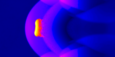
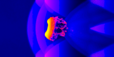
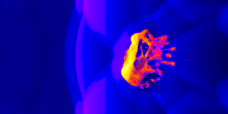
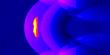
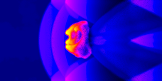
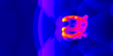
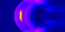
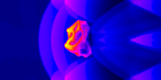
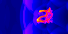
Figure 11: Results for the “blob” test. We compare projected gas densities at $t=4$, $6$ and $8$ (left, central and right panels, respectively) for GADGET (upper panels), GSPH-I02 (middle panels) and GSPH (bottom panels).

In order to further verify the performances on the blob test of different implementations of the GSPH scheme, we compare in Figure 13 the results obtained at $t=8$ for the reference GSPH scheme (upper left panel), for the GSPH-VLin version based on the linear interpolation of the volume function (upper right panel), for the GSPH-1ord version based on the first-order reconstruction for the solution of the RP (bottom left panel), and on the GSPH-CW scheme based on Eqs. (16) and (17). The result for GSPH-VLin is rather similar to that of GSPH, although the latter develops a lower degree of filamentary structures and instabilities. This result agrees with what shown in Fig. 8 for the KH test. On the other hand, the results dramatically change if we use instead the first-order reconstruction scheme of GSPH-1ord for the assignment of the thermodynamical variables at the interface. In line with the KH test result, the higher degree of diffusivity of this scheme dumps the development of instabilities, thus preserving the structure of the blob. This result highlights that, while using an accurate scheme of interpolation for the volume function has a sizable effect, a much more dramatic change is provided by properly choosing the reconstruction scheme for the RP solution. Finally, the blob test confirms the result based on the KH test on the incorrect description of the GSPH-CW scheme in describing the development of instabilities.

In order to better quantify the different efficiency that different schemes have in describing the disruption of the blob, we show in Figure 12 the evolution of the blob mass loss for our various schemes. Following Agertz et al. (2007), we define a gas particle to belong to the blob whenever its density is $\rho>0.64\rho_{cl}$, being $\rho_{cl}$ the blob density as set in the initial conditions. As expected, GADGET show the lowest degree of mass loss, a result which is in line with what shown by Agertz et al. (2007) and Heß & Springel (2010). GSPH , GSPH-VLin and GSPH-I02 have very similar mass loss rates, while GSPH-CW retains more mass at the end of our simulation. This can be understood in terms of a lesser ability of the latter scheme to capture the development of hydrodynamical instabilities, as shown in Figure 10. We also note that the strongest mass loss rate takes place for GSPH-1ord. Owing to the quite poor performance of this scheme in describing the development of the KH instability, we argue that numerical diffusion is in this case the main driver of the blob mass loss. This is also indicated by the different final shape of the blob (Figure 13). The cloud is disrupted into several pieces in the GSPH and GSPH-VLin schemes, while it retains its integrity in the GSPH-1ord and GSPH-CW ones. Therefore, significant mass loss of the blob can be obtained both through spurious numerical diffusion and through the development of genuine instabilities. However, only the latter are capable also to produce the disruption of the blob into several pieces.

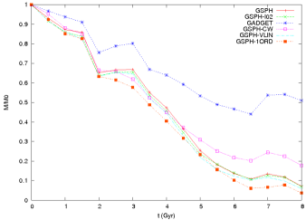
Figure 12: Mass loss of the blob as a function of time for the different hydrodynamical schemes. We define a gas particle to be part of the blob if its density is $\rho>0.64\rho_{cl}$, with $\rho_{cl}$ the initial density of the blob. Red line with crosses refer to GSPH, green ones to GSPH-I02, blue ones to GADGET, magenta ones to GSPH-CW, cyan ones to GSPH-VLin  and yellow ones to GSPH-1ord.

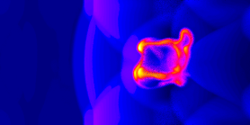
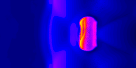
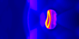
Figure 13: Comparison of the results for the “blob” test at $t=8$ for different implementations of the GSPH scheme: GSPH (upper left), GSPH-VLin (upper right), GSPH-1ord (lower left), and GSPH-CW (lower right).

5 Conclusions

In this paper we presented results of 3D standard hydrodynamical tests for different implementations of the Godunov Smoothed Particle Hydrodynamics (GSPH) within the GADGET-3  code (Springel, 2005). The conceptual difference between GSPH scheme and standard SPH scheme lies in the fact that the former is based on explicitly convolving momentum and energy equations with the interpolation kernel. The resulting equations implemented in the simulation code are exact to $O(h^{2})$. Suitable expression for momentum and energy equations to be implemented numerically are obtained by assuming a Gaussian shape for the interpolating kernel. A natural way of implementing the equations of GSPH is by solving the Riemann Problem between each pair of particles (see Inutsuka, 2002, for a detailed discussion of GSPH). Quite remarkably, solving the RP between each particle pair brings the extra benefit that no artificial viscosity is required to capture shocks, unlike in the standard SPH.

The different implementations of the GSPH scheme, that we presented in this paper (see Table 1), correspond to (a) using either linear or cubic-spline interpolation for the volume function, which provides the position of the interface where to solve the RP; (b) using either a first-order or a second-order reconstruction scheme to assign thermodynamical variables at the interface in the solution of the RP; (c) using different limiters to prevent oscillations of interpolated quantities in the RP. Furthermore, we also considered a variant of the GSPH scheme, which is not based on the convolution of the equations of fluido-dynamics, and is instead essentially based on replacing pressure and velocity in the SPH equations with the values obtained from the solution of the RP. The performances of these different implementations to describe discontinuities and development of gas-dynamical instabilities have been assessed using a shock tube test (Sod, 1978), a shear-flow test to follow Kelvin–Helmholtz (KH) instabilities and the disruption of a cold blob moving in a hot atmosphere (e.g., Agertz et al., 2007).

The results of our simulation tests can be summarised as follows.

(1)

As for the shock tube (see Fig. 2), we verified that GSPH is able to correctly follow the development of the shock, despite the fact that it does not include artificial viscosity. Furthermore, GSPH is also effective in removing the spurious “pressure blip” generated by standard SPH at the contact discontinuity, thanks to its capability to describe diffusion of entropy across the discontinuity (see Fig. 3). Quite interestingly, the best description of the discontinuity is provided by our reference GSPH scheme, rather than by the more diffusive GSPH-CW scheme. This result highlights that including thermal diffusion is not enough in itself to provide a completely correct description of discontinuities. Indeed, the more accurate description of density gradients offered by the GSPH, also significantly contribute to suppress spurious pressure forces at such discontinuities.

(2)

Unlike standard SPH, our reference GSPH scheme is quite effective in following the development of KH instabilities in the shear-flow test (see Fig. 5). We have verified that the accuracy in developing the curl structure of the instability is quite sensitive to the details of the implementation (see Fig. 8). For instance, using a first-order reconstruction dramatically degrades the GSPH performance for this test. Also using a too small number of neighbours, a linear interpolation of the volume function and the limiter by Inutsuka (2002), instead of that by van Leer (1979), also somewhat worsen, although to different degrees, the description of the KH instabilities.

(3)

Similar results also hold for the “blob test”. Also in this case, our standard GSPH implementation follows the onset of Rayleigh-Taylor and Richtmyer-Meshkov (RT, RM) and KH instabilities. As a result, the blob is dissolved much more efficiently than in SPH simulations. However, the performance of GSPH significantly worsen in case a first-order reconstruction scheme is used to assign variables at the interface. This highlights once again that diffusivity of the solution of the RP needs to be minimised to reliably follow the development of instabilities in GSPH.

In this paper we focused on the comparison between different hydrodynamical schemes, when applied to control test cases, without analysing the behaviour of each of such schemes when resolution is progressively increased (or degraded). On the other hand, it is worth reminding that a numerically diffusive scheme could converge to the correct solution when applied to test cases with sufficiently high resolution. For instance, Robertson et al. (2010) showed this to be case for the Galilean invariance in Eulerian codes, in the case of KH instabilities.

In general our results agree with and extend those presented by Cha et al. (2010) on two-dimensional KH and “blob” test of the GSPH. Our analysis highlights the important role played by reconstruction at the interface, by the choice of the limiter and by the interpolation order for the volume function (see Appendix). The remarkable improvement shown by GSPH with respect to the standard SPH to describe contact discontinuities and development of gas-dynamical instabilities makes in principle this hydrodynamic scheme highly promising for applications in computational astrophysics and cosmology.

As for its computational cost, it is worth pointing out that the need of solving the RP between each pair of particles does not represent a limiting factor. Clearly, the solution of the RP requires an iterative procedure, which in principle could increase the computational cost. This could be avoided using an approximate Riemann solver, which does not require an iterative procedure, as e.g. an Harten-Lax-van Leer-Contact (HLLC) solver.

However, the lack of artificial viscosity in the GSPH makes the Courant condition much less stringent in the shock regions than for SPH, thereby leading to a more relaxed time-stepping. We verified in our test that this compensates the overhead associated to the RP solution.

However, it is worth reminding that the GSPH equations derived by Inutsuka (2002) (see also Cha et al., 2010) and used in our implementation (Eqs. 13 and 14) hold only for a Gaussian kernel. The subsequent request for a fairly large number of neighbours and the $\sqrt{2}$ multiplicative factor in front of the kernel smoothing length in the above equations make the neighbour search quite expensive. An implementation of GSPH based instead on a kernel with compact support, like the B-spline kernel, would clearly be highly desirable to make the code more efficient for applications involving large dynamic and temporal ranges.

Appendix. Volume interpolation

In this Appendix we summarise for completeness the expressions for the interpolating volume $V_{i,j}(h)$, which appears in the GSPH equations of evolution (10) and (11), in the case of linear and of cubic spline interpolation. We will also provide the corresponding expressions for the position of the interface at which the Riemann problem between the $i$-th and the $j$-th particle is solved. A full derivation of all such expressions is provided by I02.

The linearly-interpolated expression of the specific volume at the coordinate $s$, along the axis joining the $i$-th and the $j$-th particle, is

$$V(s)=\rho(s)^{-1}=C_{i,j}s+D_{i,j}$$ (25)

where

$$C_{i,j} = {V({\bf x}_{i})-V({\bf x}_{j})\over\Delta s_{i,j}}$$

$$D_{i,j} = {V({\bf x}_{i})+V({\bf x}_{j})\over 2}\,$$ (26)

We remind that we denote with $s_{i}$ and $s_{j}$ the components of the ${\bf x}_{i}$ and ${\bf x}_{j}$ vectors along the $s$-axis, so that $\Delta s_{ij}=s_{i}-s_{j}=|{\bf x}_{i}-{\bf x}_{j}|$.

Including the above expression for $\rho^{-1}$ into the integral appearing on the l.h.s. of Eq.(12), one obtains

$$V_{i,j}^{2}\,=\,{1\over 4}h^{2}C_{i,j}^{2}+D_{i,j}^{2}\,.$$ (27)

In order to compute the position of the interface, let us define the weighted–average $f_{i,j}^{*}$ of a generic function $f({\bf x})$ through the relation

$$\int{f({\bf x})\over\rho^{2}({\bf x})}W({\bf x}-{\bf x}_{i};h)W({\bf x}-{\bf x}_{j};h)d{\bf x}=$$

$$f_{i,j}^{*}\int{1\over\rho^{2}({\bf x})}W({\bf x}-{\bf x}_{i};h)W({\bf x}-{\bf x}_{j};h)d{\bf x}\,.$$ (28)

Using then the linear approximation for $f(s)=s(f_{i}-f_{j})/\Delta s_{i,j}$ and the above linear interpolation for $\rho(s)^{-1}$, one obtains

$$f_{i,j}^{*}={f_{i}-f_{j}\over\Delta s_{i,j}}s_{i,j}^{*}+{f_{i}+f_{j}\over 2}\,.$$ (29)

In the above equation the position of the interface

$$s_{i,j}^{*}={h^{2}C_{i,j}D_{i,j}\over 2V_{i,j}^{2}(h)}$$ (30)

is defined as the position on the $s$-axis at which the linearly-interpolated function $f$ takes the value $f_{i,j}^{*}$.

The computation for a more accurate cubic–spline interpolation of the volumes proceeds in a similar way. In this case, it is

$$V(s)=\rho^{-1}(s)=A_{i,j}s^{3}+B_{i,j}s^{2}+C_{i,j}s+D_{i,j}$$ (31)

where the coefficients of the interpolating function are given by Eqs.(61) of I02. Using again Eq.(12) for the definition of $V_{i,j}$, one obtains in this case

$$V_{i,j}^{2} = {15\over 64}h^{6}A_{i,j}^{2}+{3\over 16}h^{4}(A_{i,j}C_{i,j}+B_{i,j}^{2})+$$ (32)

$$+ {1\over 4}h^{2}(2B_{i,j}D_{i,j}+C_{i,j}^{2})+D_{i,j}^{2}$$

so that the expression for the position of the interface becomes

$$s_{i,j}^{*} = {1\over V_{i,j}^{2}(h)}]\biggl{(}{15\over 32}h^{6}A_{i,j}B_{i,j}+$$ (33)

$$+ {3\over 8}h^{4}(A_{i,j}D_{i,j}+B_{i,j}C_{i,j})+{1\over 2}h^{2}C_{i,j}D_{i,j}\biggr{)}\,.$$

References

- Agertz et al. (2007) Agertz O., Moore B., Stadel J., Potter D., Miniati F., Read J., Mayer L., Gawryszczak A., Kravtsov A., Nordlund Å., Pearce F., Quilis V., Rudd D., Springel V., Stone J., Tasker E., Teyssier R., Wadsley J., Walder R., 2007, MNRAS, 380, 963
- Balsara (1995) Balsara D. S., 1995, Journal of Computational Physics, 121, 357
- Cha et al. (2010) Cha S., Inutsuka S., Nayakshin S., 2010, MNRAS, 403, 1165
- Cha & Whitworth (2003) Cha S., Whitworth A. P., 2003, MNRAS, 340, 73
- Chandrasekhar (1961) Chandrasekhar S., 1961, Hydrodynamic and hydromagnetic stability, International Series of Monographs on Physics, Oxford: Clarendon
- Cullen & Dehnen (2010) Cullen L., Dehnen W., 2010, MNRAS, pp 1126–+
- Dolag et al. (2005) Dolag K., Vazza F., Brunetti G., Tormen G., 2005, MNRAS, 364, 753
- Gingold & Monaghan (1977) Gingold R. A., Monaghan J. J., 1977, MNRAS, 181, 375
- Godunov (1959) Godunov S. K., 1959, Math. Sbornik, 47, 271
- Heß & Springel (2010) Heß S., Springel V., 2010, MNRAS, 406, 2289
- Inutsuka (2002) Inutsuka S., 2002, Journal of Computational Physics, 179, 238
- Lombardi et al. (1999) Lombardi J. C., Sills A., Rasio F. A., Shapiro S. L., 1999, Journal of Computational Physics, 152, 687
- Lucy (1977) Lucy L. B., 1977, AJ, 82, 1013
- Merlin et al. (2010) Merlin E., Buonomo U., Grassi T., Piovan L., Chiosi C., 2010, A&A, 513, A36+
- Monaghan (1997) Monaghan J. J., 1997, Journal of Computational Physics, 136, 298
- Monaghan (2005) Monaghan J. J., 2005, Reports on Progress in Physics, 68, 1703
- Monaghan & Gingold (1983) Monaghan J. J., Gingold R. A., 1983, Journal of Computational Physics, 52, 374
- Morris & Monaghan (1997) Morris J. P., Monaghan J. J., 1997, Journal of Computational Physics, 136, 41
- Price (2008) Price D. J., 2008, Journal of Computational Physics, 227, 10040
- Read et al. (2010) Read J. I., Hayfield T., Agertz O., 2010, MNRAS, 405, 1513
- Robertson et al. (2010) Robertson B. E., Kravtsov A. V., Gnedin N. Y., Abel T., Rudd D. H., 2010, MNRAS, 401, 2463
- Rosswog (2009) Rosswog S., 2009, NewAR, 53, 78
- Sod (1978) Sod G. A., 1978, Journal of Computational Physics, 27, 1
- Springel (2005) Springel V., 2005, MNRAS, 364, 1105
- Springel (2010a) Springel V., 2010a, MNRAS, 401, 791
- Springel (2010b) Springel V., 2010b, ARAA
- Springel & Hernquist (2002) Springel V., Hernquist L., 2002, MNRAS, 333, 649
- Toro (1999) Toro E., 1999, Riemann Solvers and Numerical Methods for Fluid Dynamics, 2nd edn., Interscience Tracts in Pure and Applied Mathematics no. 4. Wiley, New York
- Toro et al. (1994) Toro E. F., Spruce M., Speares W., 1994, Shock Waves, 4, 25
- Valcke et al. (2010) Valcke S., de Rijcke S., Rödiger E., Dejonghe H., 2010, MNRAS, pp 1047–+
- van Leer (1979) van Leer B., 1979, Journal of Computational Physics, 32, 101
- van Leer (1997) van Leer B., 1997, Journal of Computational Physics, 135, 229
- van Leer (2006) van Leer B., 2006, Communications in Computational Physics, 1, 192
- Wadsley et al. (2008) Wadsley J. W., Veeravalli G., Couchman H. M. P., 2008, MNRAS, 387, 427