Excitation, two-center interference and the orbital geometry in laser-induced nonsequential double ionization of diatomic molecules

Abstract

We address the influence of the molecular orbital geometry and of the molecular alignment with respect to the laser-field polarization on laser-induced nonsequential double ionization of diatomic molecules for different molecular species, namely $\mathrm{N}_{2}$ and $\mathrm{Li}_{2}$. We focus on the recollision excitation with subsequent tunneling ionization (RESI) mechanism, in which the first electron, upon return, promotes the second electron to an excited state, from where it subsequently tunnels. We show that the electron-momentum distributions exhibit interference maxima and minima due to the electron emission at spatially separated centers. We provide generalized analytical expressions for such maxima or minima, which take into account $s$ $p$ mixing and the orbital geometry. The patterns caused by the two-center interference are sharpest for vanishing alignment angle and get washed out as this parameter increases. Apart from that, there exist features due to the geometry of the lowest occupied molecular orbital (LUMO), which may be observed for a wide range of alignment angles. Such features manifest themselves as the suppression of probability density in specific momentum regions due to the shape of the LUMO wavefunction, or as an overall decrease in the RESI yield due to the presence of nodal planes.

.1 Introduction

Strong-field phenomena such as high harmonic generation (HHG) or above-threshold ionization (ATI) have been used as tools for the attosecond imaging of molecular orbitals imaging , for probing the structural changes in molecules with attosecond precision and for studying quantum interference effects due do photoelectron or high-harmonic emission at spatially separated centers Probing . This has been made possible due to the fact that both phenomena are caused by the rescattering or recombination of an electron with its parent molecule, which, for typical intense lasers, occur within hundreds of attoseconds. The simplest targets for which this interference can be studied are diatomic molecules, which can be viewed as the microscopic counterpart of a double-slit experiment doubleslit .

Potentially, laser-induced nonsequential double ionization (NSDI) can also be employed for probing molecular orbitals since laser-induced recollision plays an important role in this case. In NDSI the returning electron rescatters inelastically with its parent ion, or molecule, giving part of its kinetic energy to a second electron. This electron can be released in the continuum either through electron-impact ionization A.Becker ; Carla1 ; Carla2 ; M.Lein ; X.Liu ; prauzner ; A.Staudte ; Emanouil ; Bondar or recollision excitation with subsequent tunneling ionization (RESI) RESI1 ; RESI2 . The former recollision mechanism happens when the first electron, upon return, gives enough energy to the second electron of the target so that it can overcome the second ionization potential and reach the continuum. The latter recollision mechanism happens when the first electron, upon return, gives just enough energy to the second electron so that it can be promoted to an excited bound state, from where it subsequently tunnels.

In principle, NSDI exhibits several advantages, with regard to ATI or HHG. First, it allows one to extract more dynamic information about the system, as the type of electron-electron interaction can be identified in the electron-momentum distributions Carla1 ; Carla2 ; Emanouil . Furthermore, different rescattering mechanisms, such as electron-impact ionization or RESI, populate different regions in momentum space and hence can also be traced back from such distributions routes . Apart from that, events happening at different half cycles of the driving field can be mapped into different momentum regions. Concrete examples are NSDI with few-cycle pulses fewcycle , which lead to asymmetric electron-momentum distributions, and individual processes in NSDI of diatomic molecules F2009 . Finally, electron-electron correlation is at the essence of this phenomenon and cannot be ignored. In contrast, for high-order harmonic generation one may, to first approximation, only consider a single active electron and the highest occupied molecular orbital. In fact, only very recently have multiple orbitals and electron-electron correlation been incorporated in the modeling of molecular high-order harmonic generation CarlaBrad ; Patchkovskii ; Lin ; Olga2009 ; Haessler2010 .

For the above-mentioned reasons, NSDI of molecules is being increasingly investigated since the past few years. In fact, there has been experimental evidence that the orbital symmetry NSDIsymm and the alignment angle NSDIalign affect the shapes of the electron momentum distributions. Since then, many theoretical studies have also been performed for molecules, involving, for instance, classical trajectory methods classical , the numerical solution of the time-dependent Schrödinger equation in reduced-dimensionality models TDSEmol , and semi-analytical approaches based on the strong-field approximation Smatrix_mol ; NSDIInterference ; F2009 . Semi-analytical models for NSDI in molecules, however, focus on the electron-impact ionization rescattering mechanism.

For instance, in our previous paper NSDIInterference we addressed the influence of the orbital symmetry and the molecular alignment with respect to the laser-field polarization on NSDI of diatomic molecules for the electron-impact ionization mechanism. We showed that the electron momentum distribution exhibit interference maxima and minima due to electron emission at spatially separated centers. Such fringes were positioned at $p_{1||}+p_{2||}=const.$, i.e., parallel to the anti diagonal of the plane spanned by the electron momentum components $p_{n\parallel}$ $n=1,2$ parallel to the laser-field polarization. They were sharpest if the molecule was aligned along the direction of the field, i.e., for vanishing alignment angle. As this angle increased, the fringes got increasingly blurred until they were completely washed out for perpendicular alignment.

Apart from that, recently, several studies have found that the core dynamics, in particular excitation, is important for high-harmonic generation in molecules Olga2009 ; Haessler2010 , and in particular for attosecond imaging of matter. We expect this also to be the case for nonsequential double ionization. For that reason, in the past few years, we have focused on the RESI mechanism. We have shown that the shape of the electron momentum distributions depends very strongly on the initial and excited bound states of the second electron Shaaran ; RESIM , in fact far more critically than for electron-impact ionization Carla2 . If this is the case already for single atoms, one expects this dependence to be even more critical for molecules.

For RESI, we expect the electron momentum distributions to be affected very strongly by the geometry of the bound-state wavefunctions, not only because the excitation process strongly depends on them, but also due to the fact that the second electron is reaching the continuum by tunneling. It is by now well known that this ionization mechanism is strongly influenced by the presence of nodal planes or the directionality of a particular molecular orbital. For instance, for HHG the nodal plane of a $\pi$ state suppresses tunnel ionization when it coincides with the polarization axis (see, e.g., Olga2009 ; CarlaBrad ; Haessler2010 ; Dejan2009 ; eliot ; BradCarla ).

In the present paper, we perform a systematic analysis of quantum-interference effect in NSDI of diatomic molecules considering the RESI mechanism. We construct a semi-analytical model, based on the strong-field approximation (SFA), in which an electron tunnels from the HOMO of a neutral molecule and rescatters with the HOMO of its singly ionized counterpart. Thereby, we assume that the second electron is excited to the lowest unoccupied molecular orbital (LUMO). We investigate the influence of such orbitals and of the alignment angle on the NSDI electron momentum distributions. Specifically we choose species for which these orbitals have different geometries and parities. Furthermore, we address the question of whether well-defined interference patterns such as those observed in ATI or HHG computations may also be obtained for NSDI in the context of the RESI mechanism, and, if so, under which conditions. These are complementary studies to those performed in our recent work on RESI Shaaran ; RESIM , where we show that, for single atoms, the shapes of the electron momentum distributions carry information about the bound state from which the second electron leaves and the state to which it is excited.

This paper is organized as follows. In Sec. I we discuss the expression for the RESI transition amplitude, including its general expression  (Sec. I.1), the saddle-point equations obtained from it (Sec. I.2) and the specific prefactors for a diatomic molecule using Gaussian orbital basis sets (Sec. I.3). At the end of this section, (Sec. I.4) we derive a general two-center interference condition for the RESI mechanism. Subsequently, in Sec. II, we compute electron momentum distributions, with emphasis on the two-center interference (Sec. II.1), and the influence of different molecular orbitals (Sec. II.2). Finally, in Sec. III, we state the main conclusions to be drawn from this work.

I Strong-field approximation transition amplitude

I.1 General expressions

The SFA transition amplitude describing the RESI mechanism reads (for details on the derivation see Shaaran ).

$$M(\mathbf{p}_{n},t,t^{\prime},t^{{}^{\prime\prime}}) = \int_{-\infty}^{\infty}dt\int_{-\infty}^{t}dt^{\prime}\int_{-\infty}^{t^{\prime}}dt^{{}^{\prime\prime}}\int d^{3}k$$ (1)

$$V_{\mathbf{p}_{2}e}V_{\mathbf{p}_{1}e,\mathbf{k}g}V_{\mathbf{k}g}e^{iS(\mathbf{p}_{n},\mathbf{k},t,t^{\prime},t^{\prime\prime})},$$

with the action

$$S(\mathbf{p}_{n},\mathbf{k},t,t^{\prime},t^{{}^{\prime\prime}}) = -\int_{t}^{\infty}\frac{[\mathbf{p}_{2}+\mathbf{A}(\tau)]^{2}}{2}d\tau$$ (2)

$$-\int_{t^{{}^{\prime}}}^{\infty}\frac{[\mathbf{p}_{1}+\mathbf{A}(\tau)]^{2}}{2}d\tau$$

$$-\int_{t^{{}^{\prime}}}^{t^{{}^{\prime\prime}}}\frac{[\mathbf{k}+\mathbf{A}(\tau)]^{2}}{2}d\tau$$

$$+E_{1g}t^{{}^{\prime\prime}}+E_{2g}t^{{}^{\prime}}+E_{2e}(t-t^{{}^{\prime}})$$

and the prefactors

$$V_{\mathbf{k}g} = \left\langle\mathbf{\tilde{k}}(t^{\prime\prime})\right|V\left|\psi_{g}^{(1)}\right\rangle=\frac{1}{(2\pi)^{3/2}}$$ (3)

$$\times\int d^{3}r_{1}V_{0}(\mathbf{r}_{1})\exp[-i\mathbf{\tilde{k}}(t^{\prime\prime})\cdot\mathbf{r}_{1}]\psi_{g}^{(1)}(\mathbf{r}_{1})$$

$$V_{\mathbf{p}_{1}e\mathbf{,k}g} = \left\langle\mathbf{\tilde{p}}_{1}\left(t^{\prime}\right),\psi_{e}^{(2)}\right|V_{12}\left|\mathbf{\tilde{k}}(t^{\prime}),\psi_{g}^{(2)}\right\rangle=\frac{1}{(2\pi)^{3}}$$ (4)

$$\times\int\int d^{3}r_{2}d^{3}r_{1}\exp[-i(\mathbf{p}_{1}-\mathbf{k})\cdot\mathbf{r}_{1}]$$

$$\times V_{12}(\mathbf{r}_{1,}\mathbf{r}_{2})[\psi_{e}^{(2)}(\mathbf{r}_{2})]^{\ast}\psi_{g}^{(2)}(\mathbf{r}_{2})$$

and

$$V_{\mathbf{p}_{2}e} = \left\langle\mathbf{\tilde{p}}_{2}\left(t\right)\right|V_{\mathrm{ion}}\left|\psi_{e}^{(2)}\right\rangle=\frac{1}{(2\pi)^{3/2}}$$ (5)

$$\times\int d^{3}r_{2}V_{\mathrm{ion}}(\mathbf{r}_{2})\exp[-i\mathbf{\tilde{p}}_{2}(t)\cdot\mathbf{r}_{2}]\psi_{g}^{(2)}(\mathbf{r}_{2}).$$

Eq. (1) describes the physical process in which, at a time $t^{\prime\prime},$ the first electron tunnels from a bound state $|\psi_{g}^{(1)}>$  into a Volkov state $|\mathbf{\tilde{k}}(t^{\prime})>$. Then the released electron propagates in the continuum from $t^{\prime\prime}$ to $t^{\prime}$ , and it is driven towards its parent molecule. Upon return, the electron scatters inelastically with the core at $t^{\prime}$ and, through the interaction $V_{12},$ promotes the second electron from the bound state $|\psi_{g}^{(2)}>$ to the excited state $|\psi_{e}^{(2)}>$. Finally, at a later time $t,$ the second electron, initially in a bound excited state $|\psi_{e}^{(2)}>,$ is released by tunneling ionization into a Volkov state $|\mathbf{\tilde{p}}_{2}\left(t\right)>$. In the above-stated equations, $E_{ng}$ $(n=1,2)$ are the ionization potentials of the ground state, $E_{ne}$ $(n=1,2)$ denote the absolute values of the excited-state energies and the potentials $V_{0}(\mathbf{r}_{1})$  and $V_{\mathrm{ion}}(\mathbf{r}_{2})$  correspond to the neutral molecule and the singly ionized molecular species, respectively. Here, the final electron momenta are described by $\mathbf{p}_{n}(n=1,2).$ All the information about the binding potentials viewed by the first and second electrons and the electron-electron interaction are embedded in the form factors (3) , (5) and (4) respectively. Assuming that the electron-electron interaction depends only on the difference between the two electron coordinates, i.e., if $V_{12}(\mathbf{r}_{1,}\mathbf{r}_{2})=V_{12}(\mathbf{r}_{1-}\mathbf{r}_{2}),$ Eq. (4) may be rewritten as

$$V_{\mathbf{p}_{1}e\mathbf{,k}g} = \frac{V_{12}(\mathbf{p}_{1}-\mathbf{k})}{(2\pi)^{3/2}}$$ (6)

$$\times\int d^{3}r_{2}e^{-i(\mathbf{p}_{1}-\mathbf{k})\cdot\mathbf{r}_{2}}[\psi_{e}^{(2)}(\mathbf{r}_{2})]^{\ast}\psi_{g}^{(2)}(\mathbf{r}_{2}),$$

with

$$V_{12}(\mathbf{p}_{1}-\mathbf{k})=\frac{1}{(2\pi)^{3/2}}\int d^{3}re^{-i(\mathbf{p}_{1}-\mathbf{k})\cdot\mathbf{r}}V_{12}(\mathbf{r})$$ (7)

and $\mathbf{r=r}_{1-}\mathbf{r}_{2}.$

Within the framework of the SFA these prefactors are gauge dependent. Specifically, in the length gauge $\mathbf{\tilde{p}}_{n}\left(\tau\right)=\mathbf{p}_{n}+\mathbf{A}(\tau)$ and $\mathbf{\tilde{k}}(\tau)=\mathbf{k}+\mathbf{A}(\tau)(\tau=t^{\prime},t^{\prime\prime}),$ while in the velocity gauge $\mathbf{\tilde{p}}_{n}\left(\tau\right)=\mathbf{p}_{n}$ and $\mathbf{\tilde{k}}(\tau)=\mathbf{k}.$ This is due to the fact that the gauge transformation cancels out with the minimal coupling in the latter case. In practice, however, for the specific situation addressed in this work, both gauges lead to very similar results. This happens as the above-stated phase differences will cancel out in $V_{\mathbf{p}_{1}e,\mathbf{k}g}$, and, in $V_{\mathbf{p}_{2}e}$, $\mathbf{A}(t)\simeq 0$ for the parameter range of interest (for more details see RESIM ). In the following, unless strictly necessary, we will drop the time dependence in $\mathbf{\tilde{p}}_{n}\left(\tau\right).$

I.2 Saddle-point analysis

Subsequently, the transition amplitude (1) is solved employing saddle-point methods. For that purpose, one must find the coordinates $(t_{s},t_{s}^{\prime},t_{s}^{\prime\prime},\mathbf{k}_{s})$ for which $S(\mathbf{p}_{n},\mathbf{k},t,t^{\prime},t^{\prime\prime})$ is stationary, i.e., for which the conditions $\partial_{t}S(\mathbf{p}_{n},\mathbf{k},t,t^{\prime},t^{\prime\prime})=\partial_{t^{\prime}}S(\mathbf{p}_{n},\mathbf{k},t,t^{\prime},t^{\prime\prime})=\partial_{t^{{}^{\prime\prime}}}S(\mathbf{p}_{n},\mathbf{k},t,t^{\prime},t^{\prime\prime})=\mathbf{0}$ and $\partial_{\mathbf{k}}S(\mathbf{p}_{n},\mathbf{k},t,t^{\prime},t^{\prime\prime})=0$ are satisfied. This leads to the equations

$$\left[\mathbf{k}+\mathbf{A}(t^{\prime\prime})\right]^{2}=-2E_{1g},$$ (8)

$$\mathbf{k=}-\frac{1}{t^{\prime}-t^{\prime\prime}}\int_{t^{\prime\prime}}^{t^{\prime}}d\tau\mathbf{A}(\tau)$$ (9)

$$[\mathbf{p}_{1}+\mathbf{A}(t^{\prime})]^{2}=\left[\mathbf{k}+\mathbf{A}(t^{\prime})\right]^{2}-2(E_{2g}-E_{2e}).$$ (10)

and

$$[\mathbf{p}_{2}+\mathbf{A}(t)]^{2}=\mathbf{-}2E_{2e},$$ (11)

which, as discussed below, provide additional physical insight into the problem.

The saddle-point Eq. (8) gives the conservation of energy when the first electron tunnel ionized at a time $\ t^{\prime\prime}$. Eq. (9) constraints the intermediate momentum $\mathbf{k}$ of the first electron and it makes sure the electron returns to the side of its release, which lies at the geometrical center of molecule. Eq. (10) expresses the conservation of energy at a time $t^{\prime}$, when the first electron rescatters inelastically with its parent ion, and gives part of its kinetic energy $E_{\mathrm{ret}}(t^{\prime})=\left[\mathbf{k}+\mathbf{A}(t^{\prime})\right]^{2}/2$ to the core to excite the second electron from a state with energy $E_{2g}$ to a state with energy $E_{2e}$. Immediately after rescatering the first electron reaches the detector with momentum $\mathbf{p}_{1}$. Finally, Eq. (11) describes the fact that the second electron tunnels at time $t$ from an excited excited state $E_{2e}$ and reaches the detector with momentum $\mathbf{p}_{2}.$ As a consequence of the fact that tunneling has no classical counterpart, these equations possess no real solutions (for more details see Shaaran ).

I.3 Molecular prefactors

In this work, we consider that all molecular orbitals are frozen apart from the HOMO and the LUMO. We also assume frozen nuclei and a linear combination of atomic orbitals (LCAO) to construct approximate wave functions for the active orbitals. This implies that the molecular bound-state wave function for each electron reads

$$\psi^{(n)}(\mathbf{\mathbf{r}}_{n})=\sum_{\alpha}c_{\alpha}[\phi_{\alpha}^{(n)}(\mathbf{r}_{n}+\mathbf{R}/2)+(-1)^{l_{\alpha}+\lambda_{\alpha}}\phi_{\alpha}^{(n)}(\mathbf{r}_{n}-\mathbf{R}/2)]$$ (12)

where $R$ and $l_{\alpha}$ denote the internuclear separation and the orbital quantum numbers, respectively. The index $n=1,2$ refers to the electron in question.   The index $\lambda_{\alpha}=0$ applies to gerade symmetry and $\lambda_{\alpha}=1$ to ungerade symmetry. The binding potential of this molecule, as seen by each electron, is given by

$$V_{\varkappa}(\mathbf{r}_{n})=\mathcal{V}_{\varkappa}(\mathbf{r}_{n}-\mathbf{R}/2)+\mathcal{V}_{\varkappa}(\mathbf{r}_{n}+\mathbf{R}/2)$$ (13)

where the subscript $\varkappa=0$ or ion refers either to the neutral molecule or to its ionic counterpart, respectively, and $\mathcal{V}_{\varkappa}(\mathbf{r}_{n})=Z_{\mathrm{eff}}/r_{n}$ is the potential at each center in the molecule. Thereby, $Z_{\mathrm{eff}}$ is the effective core charge as seen by each of the two active electrons.

In this paper the wave function $\phi_{\alpha}^{(n)}$ is approximated by a Gaussian basis set,

$$\phi_{\alpha}^{(n)}(\mathbf{r}_{n})=\sum_{j}b_{j}^{(n)}x^{l_{\alpha}}y^{l_{\alpha}}z^{l_{\alpha}}\exp[-\zeta_{j}\mathbf{r}^{2}]$$ (14)

The coefficients $b_{j}$ and $c_{\alpha}$ and the exponents $\zeta_{j}$ can be extracted either from existing literature or from quantum chemistry codes. We compute these coefficients using GAMESS-UK GAMESS . In our basis set, we took only $s$ and $p$ states. This means that, in all the expressions that follow, $l_{\alpha}$ and $l_{\beta}$ are either $0$ or $1.$

The above-stated assumptions lead to the form factors

$$V_{\mathbf{p}_{1}e\mathbf{,k}g} = \frac{V_{12}(\mathbf{p}_{1}-\mathbf{k})}{(2\pi)^{3/2}}\sum_{\alpha}\sum_{\beta}[e^{i(\mathbf{p}_{1}-\mathbf{k})\cdot\mathbf{\mathbf{R}}/2}$$ (15)

$$+(-1)^{l_{\alpha}+l_{\beta}+\lambda_{\alpha}+\lambda_{\beta}}e^{-i(\mathbf{p}_{1}-\mathbf{k})\cdot\mathbf{\mathbf{R}}/2}]\mathcal{I}_{1},$$

where

$$\mathcal{I}_{1}=\int d^{3}r_{2}e^{-i(\mathbf{p}_{1}-\mathbf{k})\cdot\mathbf{r}_{2}}\phi_{\alpha}^{(2)}(\mathbf{r}_{2})^{{}^{\ast}}\phi_{\beta}^{(2)}(\mathbf{r}_{2})$$ (16)

and

$$V_{\mathbf{p}_{2}e}=\frac{4\pi}{(2\pi)^{3/2}}\sum_{\alpha}\left[e^{i\mathbf{\tilde{p}}_{2}\cdot\mathbf{R}/2}+(-1)^{l_{\alpha}+\lambda_{\alpha}}e^{-i\mathbf{\tilde{p}}_{2}\cdot\mathbf{R}/2}\right]\mathcal{I}_{2},$$ (17)

where

$$\ \ \ \ \ \ \ \ \mathcal{I}_{2}=\int d^{3}r_{2}\mathcal{V}_{0}(\mathbf{r}_{2})e^{-i\mathbf{\tilde{p}}_{2}\cdot\mathbf{r}_{2}}\phi_{\alpha}^{(2)}(\mathbf{r}_{2}).$$ (18)

In general, the form factor (3) does not affect the shape of the electron-momentum distributions. This is particularly true when the first electron tunnels from an orbital with no nodal planes, such as a $\sigma_{g}$ orbital NSDIInterference . However, one has to be careful when the electron tunnels from any orbital with at least one nodal plane, such as a $\pi$ orbital, as this would lead to a suppression of ionization for specific alignment angles.

In the following, we will write the above-stated equations as functions of the electron-momentum components $p_{n\parallel}$ and $\mathbf{p}_{n\perp}$ parallel and perpendicular to the laser-field polarization. Physically, we are investigating a diatomic molecule whose main axis is rotated of an angle $\theta$ with respect to the direction of the laser-field polarization. Hence, we are dealing with two frames of reference, i.e., the molecular frame of reference and the laser field frame of reference. The electron momenta in terms of their parallel and perpendicular components with regard to the laser-field polarization read

$$\mathbf{p}_{n}=p_{n||}\hat{e}_{z^{\prime}}+p_{n\perp}\cos\varphi\hat{e}_{x^{\prime}}+p_{n\perp}\sin\varphi\hat{e}_{y^{\prime}},$$ (19)

where we assumed that the laser field is polarized along the $z^{\prime}$ axis, the coordinates $x^{\prime}$ and $y^{\prime}$ define the plane perpendicular to the laser-field polarization and $\varphi$ is the azimuthal angle. In order, however, to compute the momentum-space wavefunctions for this molecule, we need the momentum coordinates in the frame of reference of the molecule. The molecular coordinates $x,y$ and $z$ can be obtained by a coordinate rotation around the $x$ axis. In this case, the momenta of the electrons in terms of parallel and perpendicular components in this latter frame of reference will be

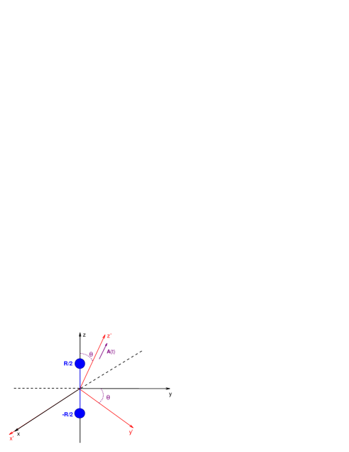
Figure 1: Schematic representation of the molecule and laser field frames of reference, represented by the black and red sets of axis $x,y,z$ and $x^{\prime},y^{\prime},z^{\prime}$ respectively. The two centers of the molecule are apart by $R$ along the $z$ axis of the molecule, and their positions are indicated by the blue circles in the figure. The field $\mathbf{A}(t)$ is polarized along the $z^{\prime}$ axis, and $\theta$ shows the alignment angle of the molecule with respect to the laser field.

$$\mathbf{p}_{n} = (p_{n||}\cos\theta+p_{n\perp}\sin\theta\sin\varphi)\hat{e}_{z}+p_{n\perp}\cos\varphi\hat{e}_{x}$$ (20)

$$\text{ \ }+(p_{n\perp}\cos\theta\sin\varphi-p_{n||}\sin\theta)\hat{e}_{y}.$$

This implies that the momentum components $p_{nx},p_{ny}$ and $p_{nz}$ are defined by Eq. (20) and that

$$\mathbf{p}_{n}\cdot\mathbf{\mathbf{R}}/2=(p_{n||}\cos\theta+p_{n\perp}\sin\theta\sin\varphi)R/2.$$ (21)

A schematic representation of both the field and molecular sets of coordinates is presented in Fig. 1. Below, we provide the explicit expressions for the integrals $\mathcal{I}_{n}(n=1,2)$ in the prefactors (15) and (17), for the specific types of orbitals employed in this work.

I.3.1 Excitation $\sigma\rightarrow\sigma$

If the second electron is excited from a $\sigma$ to a $\sigma$ orbital, both integrals will have the forms

$$\mathcal{I}_{1} = \sum_{j,j^{\prime}}\frac{b_{j}^{(1)}b_{j^{\prime}}^{(1)}\pi^{3/2}(-i)^{l_{\alpha}+l_{\beta}}}{2^{{}^{l_{\alpha}+l_{\beta}}}(\zeta_{j}+\zeta_{j^{\prime}})^{3/2+l_{\alpha}+l_{\beta}}}$$ (22)

$$\text{ \ \ \ }\times\exp[-\frac{(\mathbf{p}_{1}-\mathbf{k})^{2}}{4(\zeta_{j}+\zeta_{j^{\prime}})}].\Upsilon(l_{\alpha},l_{\beta})$$

where

$$\Upsilon(l_{\alpha},l_{\beta})=\left\{\begin{array}[]{c}1,\text{ \ \ \ }l_{\alpha}+l_{\beta}=0\\ (\mathbf{p}_{1}-\mathbf{k})_{z},\text{\ \ \ }l_{\alpha}+l_{\beta}=1\\ 2(\zeta_{j}+\zeta_{j^{\prime}})-(\mathbf{p}_{1}-\mathbf{k})^{2}_{z},\text{ \ \ }l_{\alpha}+l_{\beta}=2\end{array}\right.,$$ (23)

and

$$\mathcal{I}_{2}=\sum_{j^{\prime}}b_{j^{\prime}}^{(2)}(-i)^{l_{\beta}}G(l_{\beta}),$$ (24)

where

$$G(l_{\beta})=\left\{\begin{array}[]{c}2\sqrt{\pi}I_{r}^{(l_{\alpha}=0)},l_{\beta}=0\\ \left(\tilde{p}_{2z}/\tilde{p}_{2}\right)I_{r}^{(l_{\alpha}=1)},l_{\beta}=1\end{array}\right..$$ (25)

In Eq. (25), $I_{r}^{(l_{\alpha}=0)}$ and $I_{r}^{(l_{\alpha}=1)}$ indicate the radial integrals

$$I_{r}^{(l_{\alpha})}=\int_{0}^{\infty}r^{l_{\beta}+1}j_{l_{\beta}}(\tilde{p}_{2}r)\exp[-\zeta_{j}r^{2}]dr,$$ (26)

where $j_{l_{\beta}}(\tilde{p}_{2}r)$ denotes spherical Bessel functions.

I.3.2 Excitation $\sigma\rightarrow\pi$

We also consider that the second electron is excited from a $\sigma$ orbital to a $\pi$ orbital. In this case, these orbitals are degenerate. For that reason, we choose to consider a coherent superposition of the $\pi_{x}$ and $\pi_{y}$ orbitals carrying equal weights. This gives

$$\mathcal{I}_{1} = \sum_{j,j^{\prime}}b_{j}^{(1)}b_{j^{\prime}}^{(1)}\pi^{3/2}\left[(-i(\mathbf{p}_{1}-\mathbf{k})_{y})^{l_{\beta}}+(-i(\mathbf{p}_{1}-\mathbf{k})_{x})^{l_{\beta}}\right]$$ (27)

$$\text{ \ }\frac{(-i(\mathbf{p}_{1}-\mathbf{k})_{z})^{l_{\alpha}}}{2^{{}^{l_{{}_{\alpha}}+l_{\beta}}}(\zeta_{j}+\zeta_{j^{\prime}})^{3/2+l_{\alpha}+l_{\beta}}}\exp[-\frac{(\mathbf{p}_{1}-\mathbf{k})^{2}}{4(\zeta_{j}+\zeta_{j^{\prime}})}].$$

One should note that, if the electron is excited from a $\pi$ to a $\sigma$ orbital, $\mathcal{I}_{1}$ will also have this form. In the second prefactor,

$$\mathcal{I}_{2}=\sum_{j^{\prime}}b_{j^{\prime}}^{(2)}(-i)^{l_{\beta}}\left[\frac{(\tilde{p}_{2y})^{l_{\beta}}+(\tilde{p}_{2x})^{l_{\beta}}}{\tilde{p}_{2}}\right]I_{r}^{(l_{\beta})},$$ (28)

with $l_{\beta}=1$. Throughout, $(\mathbf{p}_{1}-\mathbf{k})_{\varkappa}$ and $\tilde{p}_{2\varkappa},$ with $\varkappa=x,y,z$ are defined according to Eq. (20).

I.4 Interference Condition

Here we provide a general interference condition, which takes into account the structure of the orbitals. This includes $s$ $p$ mixing and the orbital parity. The expressions that follow are easily derived if the exponentials in Eqs. (15) and (17) are expanded in terms of trigonometric functions. In this case, the prefactor (15) can be written as

$$V_{\mathbf{p}_{1}e\mathbf{,k}g}=\frac{V_{12}(\mathbf{p}_{1}-\mathbf{k})}{(2\pi)^{3/2}}\sum_{\alpha}\sum_{\beta}\sqrt{C_{+}^{2}-C_{-}^{2}}\sin[\xi_{1}+(\mathbf{p}_{1}-\mathbf{k})\cdot\mathbf{R}/2]\mathcal{,}$$ (29)

with

$$\xi_{1}\mathbf{=}\arctan[\frac{-iC_{+}}{C_{-}}]\text{\ \ \ }$$ (30)

and

$$C_{\pm}=1\pm(-1)^{l_{\alpha}+l_{\beta}+\lambda_{\alpha}+\lambda_{\beta}}.\text{\ }$$ (31)

A similar procedure for high-order harmonic generation has been adopted in Dejan2009 . Interference minima are present if

$$\xi_{1}+(\mathbf{p}_{1}-\mathbf{k})\cdot\mathbf{R}/2\mathbf{=}m\pi\text{,\ \ }$$ (32)

where $m$ is an integer. Similarly, interference maxima are obtained for

$$\xi_{1}+(\mathbf{p}_{1}-\mathbf{k})\cdot\mathbf{R}/2\mathbf{=}(2m+1)\pi/2\text{.\ }$$ (33)

We will focus on the minima given by Eq. (32) as they are much easier to observe. If this equation is written in terms of the electron momentum component $(\mathbf{p}_{1}-\mathbf{k})_{z}$ parallel to the molecular axis we find

$$\left[(p_{1||}-k)\cos\theta+p_{1\perp}\sin\theta\sin\varphi\right]R/2=m\pi-\xi_{1}.$$ (34)

The above-stated equation shows that the parallel momentum component $p_{1||}$ parallel to the laser-field polarization will lead to well-defined interference fringes approximately at

$$p_{1||}=\frac{2(m\pi-\xi_{1})}{R\cos\theta}+k.$$ (35)

This means that, in the plane $p_{1||}p_{2||}$, these minima will be at $p_{1||}=const.,$ i.e., parallel to the $p_{1||}$ axis. The perpendicular component $p_{1\perp}$ will mainly cause a blurring in such fringes, when the azimuthal angle is integrated over. Extreme limits will be found for alignment angle $\theta=0$, with sharp two-center patterns, and $\theta=90^{\circ},$ when they get washed out.

Following the same line of argument,

$$V_{\mathbf{p}_{2}e}=\frac{4\pi}{(2\pi)^{3/2}}\sum_{\alpha}\sqrt{D_{+}^{2}-D_{-}^{2}}\sin[\xi_{2}+\mathbf{\tilde{p}}_{2}\cdot\mathbf{R}/2]\mathcal{I}_{2},$$ (36)

with

$$\xi_{2}\mathbf{=}\arctan[\frac{-iD_{+}}{D_{-}}]\text{\ \ \ }$$ (37)

and

$$D_{\pm}=1\pm(-1)^{l_{\beta}+\lambda_{\beta}}\ \text{\ \ .}$$ (38)

Interference minima are present for Eq. (36) if

$$\xi_{2}+\mathbf{\tilde{p}}_{2}\cdot\mathbf{R}/2\mathbf{=}m\pi$$ (39)

Likewise, there will be interference fringes for

$$\tilde{p}_{2||}=\frac{2(m\pi-\xi_{2})}{R\cos\theta},$$ (40)

i.e., parallel to the $p_{2||}$ axis in the plane spanned by the parallel momentum components $p_{1||},$ $p_{2||}$. In the velocity and the length gauges, $\tilde{p}_{2||}=p_{2||}$ and $p_{2||}+A(t),$ respectively. Since, however, $A(t)\simeq 0$ for the electron tunneling time, in practice there will be very little difference. The perpendicular momentum components will lead to a blurring in the fringes.

II Electron momentum distributions

In this section, we compute electron momentum distributions, as functions of the momentum components $(p_{1\parallel},p_{2\parallel})$ parallel to the laser-field polarization. We assume the external laser field to be a monochromatic wave linearly polarized along the axis $z^{\prime}$. Explicitly,

$$\mathbf{E}(t)=\varepsilon_{0}\sin\omega t\hat{e}_{z^{\prime}}.$$ (41)

This approximation is reasonable for laser pulses of the order of ten cycles or longer X.Liu . These distributions, when integrated over the transverse momentum components, read

$$F(p_{1\parallel},p_{2\parallel}) = \iint d^{2}p_{1\perp}d^{2}p_{2\perp}|M_{R}(\mathbf{p}_{1},\mathbf{p}_{2})$$

$$+ M_{L}(\mathbf{p}_{1},\mathbf{p}_{2})+\mathbf{p}_{1}\leftrightarrow\mathbf{p}_{2}|^{2},$$

where $M_{R}(\mathbf{p}_{1},\mathbf{p}_{2})$ and $M_{L}(\mathbf{p}_{1},\mathbf{p}_{2})$ refer to the right and left peak in the electron momentum distributions, respectively, the transition amplitude $M_{R}(\mathbf{p}_{1},\mathbf{p}_{2})$ is given by Eq. (1), and $d^{2}p_{n\perp}=$ $p_{n\perp}dp_{n\perp}d\varphi_{p_{n}}.$ For a monochromatic field, we can use the symmetry $\mathbf{A}(t)=-\mathbf{A}(t\pm T/2),$ where $T=2\pi/\omega$ corresponds to a field cycle, in order to simplify the computation of  the electron momentum distributions. This is explained in detail in our previous work RESIM . We also symmetrize the above-stated distributions with respect to the particle exchange $\mathbf{p}_{1}\leftrightarrow\mathbf{p}_{2}.$ To a good approximation, it is sufficient to consider the incoherent sum in Eq. (II) as the interference terms between the right and left peaks practically get washed out upon the transverse momentum integration (see Appendix B in RESIM ).

In the following, we will compute electron momentum distributions for $\mathrm{Li}_{2}$ and $\mathrm{N}_{2}.$ For all cases, we assume that the electron-electron interaction is of contact type, i.e., $V_{12}=\delta(\mathbf{r}_{1}-\mathbf{r}_{2}).$ This will avoid a further momentum bias in the electron-electron distributions as it leads to $V_{12}(\mathbf{p}_{1}-\mathbf{k})=const.$ and allow us to investigate the influence of the target structure alone. For a long-range potential, $V_{12}(\mathbf{p}_{1}-\mathbf{k})$ would be momentum dependent, and hence mask the features we intend to investigate.

II.1 Interference effects and s p mixing

We will commence by investigating whether the interference conditions derived in Sec. I.4 hold. For that purpose, we must have non-negligible tunneling ionization for parallel-aligned molecules, as this is the situation for which the fringes are expected to be sharpest. Hence, one must consider a target for which neither the HOMO nor the LUMO exhibits nodal planes along the internuclear axis. Therefore, we assume that the first electron tunnels from the HOMO in $\mathrm{Li}_{2}$ and rescatters inelastically with $\mathrm{Li}_{2}^{+},$ exciting the second electron from its HOMO (2$\sigma_{g})$ to its LUMO (2$\sigma_{u})$. In order to get a clear picture of conditions (32) and (39), we must investigate the corresponding prefactors individually.

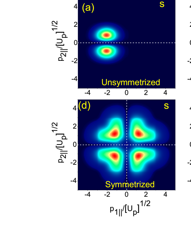
Figure 2: Electron-momentum distributions for NSDI in $\mathrm{Li}_{2}$ (bound-state energies $E_{1g}$ $=$ $0.18092040$ a.u., $E_{2g}$ $=$ $0.43944428$ a.u. and $E_{2e}$ $=$ $0.12481836$ a.u. and equilibrium internuclear distance $R=4.7697$ a.u.) considering only the RESI mechanism, as functions of the momentum components parallel to the laser-field polarization, obtained considering $V_{\mathbf{p}_{2}e}$ according to Eq. (5) and $V_{\mathbf{p}_{1}e,\mathbf{k}g}=const$. We consider zero alignment angle, driving-field intensity $I=4.6\times 10^{13}\mathrm{W/cm}^{2}$ and $\omega=0.057$ a.u. respectively. Panels (a) to (c) display only the contribution from the orbits starting in the first half cycle of the field, while in panels (d) to (f) the distributions have been symmetrized to account for the electron orbits starting in the other half cycle and for electron indistinguishability. The left, middle and right panels correspond to the contributions of the $s$, $p$ and all states used in the construction of the $\sigma_{u}$ LUMO, respectively. The solid, dashed and short dashed lines show the position of minima due to the two-center interference, node of the wavefunction and mixed cases, respectively. The contour plots have been normalized to the maximum probability in each panel.

In Fig. 2, we depict the above-mentioned electron-momentum distributions for alignment angle $\theta=0^{\circ}.$ We consider $V_{\mathbf{p}_{1}e\mathbf{,k}g}=const.$ and focus on the influence of $V_{\mathbf{p}_{2}e}$ alone. We take either the individual contributions of $s$ and $p$ states or the combination of both for 2$\sigma_{u}$. For clarity, in the upper panels, we also exhibit the distributions obtained without symmetrizing with respect to the momentum exchange and electron start times. For all cases, the two-center fringes in Fig. 2 are parallel to $p_{2||}=const.$, in agreement with the second interference condition derived in Sec. I.4.

For pure $s$ or $p$ states and $\lambda_{\alpha}=1$, which is the case for a $\sigma_{u}$ orbital, this condition can be further simplified. It reduces to

$$\sin[\mathbf{\tilde{p}}_{2}\cdot\mathbf{R}/2]=0,$$ (43)

for $s$ states, and

$$\cos[\mathbf{\tilde{p}}_{2}\cdot\mathbf{R}/2]=0$$ (44)

for $p$ states. This implies that, for the former, we expect minima at $\mathbf{\tilde{p}}_{2}\cdot\mathbf{R}=2m\pi,$ while for the latter they should occur at $\mathbf{\tilde{p}}_{2}\cdot\mathbf{R}=(2m+1)\pi.$ The position of such minima can also be determined analytically by considering that the second electron tunnels at the peak of the laser field, i.e., at $t=\pi/2$. The dashed lines in the figure show that the position of these minima exhibit a very good agreement with this simple estimate. Physically, this good agreement may be attributed to the fact that the second electron tunnels most probably at this time.

For the $s$ states the two-center interference gives a sharp minimum at $p_{2\parallel}=0$ (Figs. 2 (a) and (d)), while for the $p$ states these patterns are located near $p_{2\parallel}=\pm 3\sqrt{U_{p}}$ (Figs. 2 (b) and (e)). In the $p-$state case the distribution has another minimum at $p_{2\parallel}=0,$ which comes from the fact the $p$ wavefunctions vanish for $\mathbf{p}_{n}=0$. This causes a suppression in the transition amplitude. If the contributions of both $s$ and $p$ states are considered, the minima in the high-momentum region due to the two-center interference seen for the $p$ states vanish, but the minimum at $p_{2\parallel}=0$ survives. This is shown in Figs. 2.(c) and (f) for unsymmetrized and symmetrized distributions, respectively.

One should note, however, that for parallel-aligned molecules, both the two-center minimum for the $s$ states and the minimum caused by the node in the $p$ states occur at the same momentum, i.e., at $p_{2\parallel}=0$. Hence, when $s$ $p$ mixing is included both mechanisms contribute to the suppression at the axes $p_{n\parallel}=0$ seen in Figs. 2.(c) and (f). We will now investigate the behavior of this node when the alignment angle is varied. Since for Li₂ both the LUMO and the HOMO exhibit distinct shapes and symmetries one can expect significant changes in the electron-momentum distributions when this angle is modified.

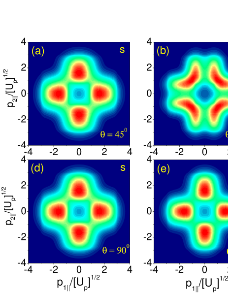
Figure 3: Electron-momentum distributions for RESI in $\mathrm{Li}_{2}$ as functions of the electron momentum components parallel to the laser-field polarization considering $V_{\mathbf{p}_{1}e,\mathbf{k}g}=const$ and $V_{\mathbf{p}_{2}e}$ according to Eq. (5), for alignment angles $\theta=45^{0}$ (panels (a) to (c)), and $90^{0}$ (panels (d) to (f)). The remaining parameters are the same as in the previous figures. The solid lines show the position of minima due to the node of the one-center wavefunction. From left to right, we considered the contributions of the $s$, $p$ and all states used in the construction of the LUMO. All panels have been symmetrized with regard to the electron orbits and indistinguishability. The contour plots have been normalized to the maximum probability in each panel.

Hence, in Fig. 3, we consider the same prefactors as in the previous case, but alignment angles $\theta=45^{0}$ and $90^{0}$. The figure shows that the patterns caused by the electron emission at spatially separated centers get washed out for such angles. This is due to the momentum components perpendicular to the laser-field polarization, and can be seen very clearly in Fig. 3.(a), where the $s$ contributions are displayed for $\theta=45^{\circ}$. Already for this angle the interference minima at the axes $p_{n\parallel}=0$ are absent. In contrast, the suppression at the axes caused by the fact that the $p$ wavefunctions vanish in that momentum region is still present. This is shown in Fig. 3.(b), in which the contributions from the $p$ states are depicted. The blurring is caused by the fact that, in momentum space, these wavefunctions are proportional to $G(l_{\beta}=1)$ (see Eq. (25)). This function contains components of $\mathbf{p}_{2}$ both parallel and perpendicular to the laser field polarization, and the contributions from the latter tend to wash out the minimum. When both $s$ and $p$ contributions are considered, there is a strong suppression of the yield near the $p_{n\parallel}=0$ axis (see Fig. 3.(c)). We have verified that this is due to the destructive interference between both types of contributions in this momentum region.

For $\theta=90^{\circ}$, only the components $p_{2\perp}$ contribute, and the electron momentum distributions are determined by the momentum-space integration alone. As a result, they reflect the momentum-space constraints for the RESI mechanism. These constraints lead to electron momentum distributions peaked at $(p_{i\parallel},p_{j\parallel})=(\pm 2\sqrt{U_{p}},0)$, with $i,j=1,2$ and $i\neq j$ and with widths $2\sqrt{U_{p}}$, and have been explicitly written in Shaaran ; RESIM . This holds both for the $s$, $p$ and mixed case (Figs. 3.(d), (e) and (f), respectively).

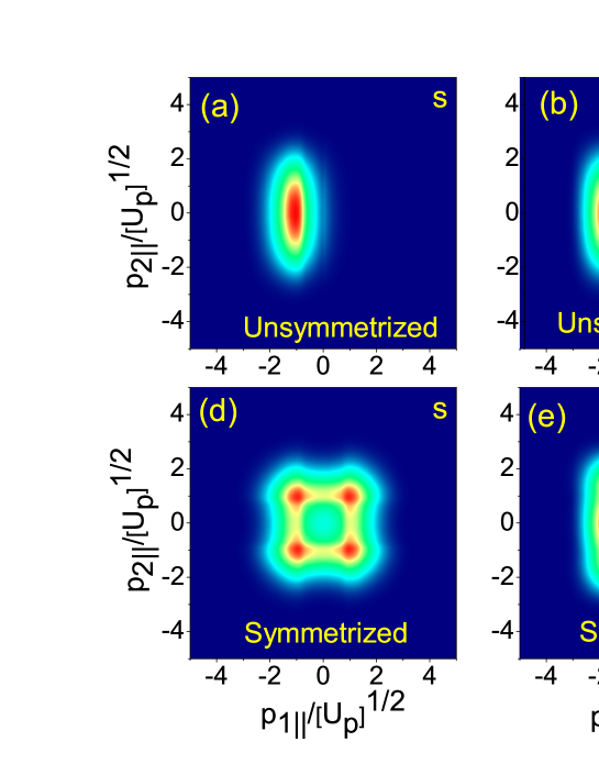
Figure 4: RESI electron-momentum distributions for $\mathrm{Li}_{2}$ considering $V_{\mathbf{p}_{2}e}=const.$ and $V_{\mathbf{p}_{1}e,\mathbf{k}g}$ according to Eq. (15), for $\theta=0$. The field and molecular parameters are the same as in the previous figure. The upper panels display only the contribution from the sets of orbits starting in the first half cycle of the laser field. In the lower panels the distributions have been symmetrized in order to account for the orbits starting in the other half cycle of the field, and for electron indistinguishability. The left, middle and right panels display the contributions from $s$, $p$ and all states composing the HOMO and the LUMO, respectively. The dashed line shows the position of the two-center interference minimum. The contour plots have been normalized to the maximum probability in each panel.

We will now focus on the interference condition determined by the excitation prefactor (4). With this objective, we will keep $V_{\mathbf{p}_{2}e}=const.$ and investigate the influence of $V_{\mathbf{p}_{1}e,\mathbf{k}g}$ alone, starting from vanishing alignment angle. Once more, we will study the contributions of the $s$ and $p$ states, and the overall distributions. The interference condition and also the wavefunctions in the excitation prefactor now incorporate the HOMO and the LUMO (see Eq. (4)). For $\mathrm{Li}_{2}^{+},$ the former and the latter are a gerade and an ungerade orbital, so that $\lambda_{\alpha}=0$ and $\lambda_{\beta}=1$ in Eq. (32). For pure $s$ states, $l_{\alpha}=l_{\beta}=0$ and for pure $p$ states, $l_{\alpha}=l_{\beta}=1.$ This will lead to the simplified interference condition

$$\sin[\mathbf{(p}_{1}-\mathbf{k)}\cdot\mathbf{R}/2]=0$$ (45)

for both. Hence, one expects a minimum close to vanishing parallel momenta in the pure cases. When $s$ $p$ mixing is included, however, different angular momenta will also be coupled and the general interference condition must be considered.

The electron momentum distributions obtained in this way are shown in Fig. 4, for both symmetrized and unsymmetrized distributions (upper and lower panels, respectively). For most distributions in the figure, we do not observe a clear suppression of the probability densities in any momentum region. This holds both for those caused by the two center interference and by the geometry of the wavefunctions at the ions. We have only observed a two center minimum if we consider the individual contributions of the $p$ states, and do not symmetrize the distributions (see Fig. 4.(b)). This is due to the fact that, for the parameters considered in this work, the two-center minimum according to condition (35) lies at or beyond the boundary of the momentum region for which rescattering of the first electron has a classical counterpart. The center of this region is roughly at $p_{1||}\simeq 2\sqrt{U_{p}}$ and its extension is determined by the difference between the maximal electron kinetic energy upon return and the excitation energy $E_{2g}-E_{2e},$ as discussed in our previous article RESIM .

Apart from that, $s$ $p$ mixing will lead to a blurring of this minimum, as it couples states with different angular momenta. Symmetrization introduces other events, either due to the electron indistinguishability or displaced by half a cycle, and obfuscates this minimum further, as shown in the lower panels of the figure.

If the alignment angle is varied, incorporating only the excitation prefactor $V_{\mathbf{p}_{1}e,\mathbf{k}g}$ will lead to ring-shaped distributions, regardless of whether only $p$, $s$ or all basis states employed in the construction of the HOMO and LUMO are taken. This is expected as, apart from the above-mentioned $s$ $p$ mixing, which blur wavefunction-specific features, there will now be transverse momentum components in the prefactor $V_{\mathbf{p}_{1}e,\mathbf{k}g}$ which will wash out two-center interference patterns. We have verified that this is indeed the case (not shown).

II.2 Molecular orbital signature

In this section, we make an assessment of how the geometry of the HOMO and the LUMO affect the RESI electron momentum distributions. With this objective, we incorporate both prefactors $V_{\mathbf{p}_{2}e}$ and $V_{\mathbf{p}_{1}e,\mathbf{k}g}$ and vary the alignment angle. In order to discuss the influence of nodal planes, we are also providing the overall yield obtained in our computation in the two figures that follow (see color maps on the right-hand side of each panel). From other strong-field phenomena, it is well-known that the presence of nodal planes may suppress the yield considerably Dejan2009 ; CarlaBrad .

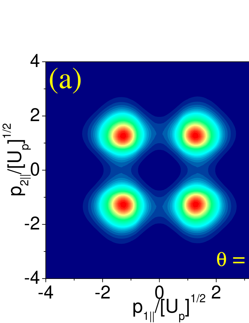
Figure 5: Electron-momentum distributions for Li₂ as functions of the parallel momenta $(p_{1\parallel},p_{2\parallel})$ considering all prefactors, for different alignment angles. Panel (a), (b) and (c) correspond the alignment angle $\theta$= 0,45 and 90 degrees, respectively. The field and molecular parameters are the same as in the previous figures.

We will commence by having a closer look at $\mathrm{Li}_{2}$. Such results are displayed in Fig. 5. The main conclusion to be drawn from the figure is that the prefactor $V_{\mathbf{p}_{2}e}$ plays the dominant role in determining the shapes of the electron momentum distributions. This can be observed by a direct comparison of Fig. 5.(a) with Fig. 2.(f), for vanishing alignment angle. The distributions in both figures exhibit similar shapes and minima at the axes $p_{n||}=0$, and are very different from those obtained if only the recollision-excitation prefactor is included (see Fig. 4(f)). The main effect of the excitation prefactor $V_{\mathbf{p}_{1}e,\mathbf{k}g}$ is to alter the widths of the distributions. This situation persists for larger angles, such as $\theta=45^{\circ}$ and $\theta=90^{\circ},$ as a comparison of Figs. 5.(b) and (c), with Fig. 3.(c) and (f) shows. For $\theta=45^{\circ}$, there is a suppression of the yield near the axes $p_{n\parallel}=0$, while for $\theta=90^{\circ}$ the interference patterns are washed out.

Another interesting feature is that the overall yield decreases with the alignment angle between the molecular axis and the field. This is due to the fact that the LUMO, from which the second electron tunnels, is a $\sigma$ orbital. Spatially, $\sigma$ orbitals are localized along the internuclear axis, and do not exhibit nodal planes for vanishing alignment angle. This implies that tunneling ionization is favored when the LUMO is parallel to the laser field, and decreases when the difference between the orientation between the field and the LUMO increases.

A legitimate question is, however, how the shape of the molecular orbital to which the second electron is excited is imprinted on the electron momentum distribution, if there are nodal planes parallel or perpendicular to the molecular axis. For that reason, we now present electron momentum distributions under the assumption that the second electron is excited to a $\pi_{g}$ orbital. Specifically, we choose $\mathrm{N}_{2}$ and its singly ionized counterpart, i.e., $\mathrm{N}^{+}_{2}$ as the molecular species in our RESI computation. The first electron will be ripped off from the HOMO, which is a $3\sigma_{g}$ orbital. However, upon return, it will excite the second electron to the LUMO, which is a $1\pi_{g}$ orbital. A $1\pi_{g}$ orbital exhibits two nodal planes, which will be oriented along the laser-field polarization for parallel and perpendicular-aligned molecules, i.e., at alignment angles $\theta=0^{\circ}$ and $\theta=90^{\circ}$. This orbital also exhibits lobes at angles $\theta=(2n+1)\pi/4$ with regard to the internuclear axis.

The results obtained for this molecular species are exhibited in Fig. 6. As an overall pattern, we observe that the NSDI signal no longer decreases monotonically with increasing alignment angle. In fact, the signal increases for alignment angle $0<\theta<45^{\circ}$, is strongest for $\theta=45^{\circ}$, and decreases once more for $45^{\circ}<\theta<90^{\circ}$. This may be easily understood as a consequence of the geometry of the $1\pi_{g}$ orbital. For $\theta=0^{\circ}$ (Fig. 6(a)), the external field is parallel to one of the nodal planes. Hence, tunnel ionization is strongly suppressed. This reflects itself in the overall yield. As the alignment angle increases, the field-polarization direction gets further and further away from the direction of this nodal plane, and the yield increases until $\theta=45^{\circ}$ (Fig. 6(b)). For this angle, the field is parallel to one of the lobes of the $1\pi_{g}$ orbital, so that tunnel ionization of the second electron is enhanced. As the alignment angle is further increased, the direction of the field approaches the nodal plane at $\theta=\pi/2$ and ionization is further suppressed (Fig. 6(c)).

Apart from the above-mentioned behavior, we also observe a suppression along the axes $p_{n\parallel}=0$, regardless of the alignment angle. This is due to the fact that, in position space, $\pi$ orbitals vanish at the origin of the coordinate system. Consequently, their Fourier transform vanish for $p_{n\parallel}=0$.

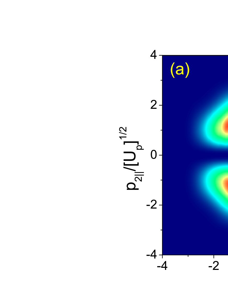
Figure 6: Electron-momentum distributions for $\mathrm{N}_{2}$ (bound-state energies $E_{1g}=0.63486$ a.u., $E_{2g}=1.12657$ a.u., and $E_{2e}=0.26871290$ a.u. and equilibrium internuclear distance $R=2.11$ a.u.) in a linearly polarized monochromatic field of intensity $I=1.25\times 10^{14}\mathrm{W}/\mathrm{cm}^{2}$ as functions of the parallel momenta $(p_{1\parallel},p_{2\parallel})$ considering all prefactors, for alignment angles $\theta=0$, $45$ and $90$ degrees(panels (a), (b) and (c), respectively).

III Conclusions

The results presented in the previous sections illustrate the potential of laser-induced nonsequential double ionization for the attosecond imaging of molecules. This is particularly true if the recollision-excitation with subsequent tunneling ionization (RESI) pathway is dominant. The computations in this work show that the shapes of the RESI electron momentum distributions depend in a dramatic fashion on the geometry of the state to which the second electron has been excited by the first electron, and from which it tunnels. The state in which the second electron is initially bound, i.e., the highest occupied molecular orbital (HOMO) of the singly ionized species plays only a secondary role.

Thereby, two main issues are important in determining the shapes of the electron momentum distribution: the quantum interference caused by the interference due to the photoelectron emission at spatially separated center, and the geometry of the orbital from which the second electron tunnels.

In order to investigate the first issue, generalized interference conditions for the first and second electron that take into account $s$ $p$ mixing along the lines of Dejan2009 have been derived, and led to fringes parallel to the $p_{n\parallel}=0$ $n=1,2$ axes in the plane spanned by the electron momentum components parallel to the laser-field polarization. These fringes agreed well with analytic estimates, but were washed out for relatively small alignment angles.

In contrast, the features caused by the orbital geometry, such as suppression of the probability density near $p_{n\parallel}=0$ observed for $p$ states were present over a wide range of alignment angles. Furthermore, the presence or absence of nodal planes manifests itself as the suppression, or enhancement, of the overall yield with regard to the alignment angle. We have discussed the differences and similarities between $\sigma_{u}$ and $\pi_{g}$ orbitals in this context, exemplified by the LUMOs of $\mathrm{N}_{2}$ and $\mathrm{Li}_{2}$. These results agree with those reported in the literature for phenomena such as high-order harmonic generation CarlaBrad ; Olga2009 ; Haessler2010 and above-threshold ionization Lin .

Acknowledgements: This work has been financed by the UK EPSRC (Grant no. EP/D07309X/1) and by the STFC. We are grateful to P. Sherwood, J. Tennyson and M. Ivanov for useful comments, and to M. T. Nygren for his collaboration in the early stages of this project. C.F.M.F. and B.B.A. would like to thank the Daresbury Laboratory for its kind hospitality.

References

- (1) J. Itatani, J. Levesque, D. Zeidler, H. Niikura, H. Pépin, J. C. Kieffer, P. B. Corkum and D. M. Villeneuve, Nature 432, 867 (2004).
- (2) H. Niikura, F. Légaré, R. Hasbani, A. D. Bandrauk, M. Yu. Ivanov, D. M. Villeneuve and P. B. Corkum, Nature 417, 917 (2002); H. Niikura, F. Légaré, R. Hasbani, M. Yu. Ivanov, D. M. Villeneuve and P. B. Corkum, Nature 421, 826 (2003); S. Baker, J. S. Robinson, C. A. Haworth, H. Teng, R. A. Smith, C. C. Chirilă, M. Lein, J. W. G. Tisch, J. P. Marangos, Science 312, 424 (2006)
- (3) M. Lein, N. Hay, R. Velotta, J. P. Marangos, and P. L. Knight, Phys. Rev. Lett. 88, 183903 (2002); Phys. Rev. A 66, 023805 (2002); M. Spanner, O. Smirnova, P. B. Corkum and M. Y. Ivanov, J. Phys. B 37, L243 (2004).
- (4) A. Becker and F. H.M. Faisal, Phys. Rev. Lett. 84, 3546 (2000); 89, 193003 (2002); S. V. Popruzhenko and S. P. Goreslavskii, J. Phys. B 34, L239 (2001); S. P. Goreslavski and S. V. Popruzhenko, Opt. Express 8, 395 (2001); S. P. Goreslavskii, S. V. Popruzhenko, R. Kopold, andW. Becker, Phys. Rev. A 64, 053402 (2001).
- (5) C. Figueira de Morisson Faria, H. Schomerus, X. Liu, and W. Becker, Phys. Rev. A 69, 043405 (2004).
- (6) C. Figueira de Morisson Faria, and M. Lewenstein, J. Phys. B 38, 3251 (2005).
- (7) M. Lein, E. K. U. Gross, and V. Engel, Phys. Rev. Lett. 85, 4707 (2000); J. Phys. B 33, 433 (2000); J. S. Parker, B. J. S. Doherty, K. T. Taylor, K. D. Schultz, C. I. Blaga, and L. F. DiMauro, Phys. Rev. Lett. 96, 133001 (2006).
- (8) X. Liu and C. Figueira de Morisson Faria, Phys. Rev. Lett. 92, 133006 (2004); C. F. Faria, X. Liu, A. Sanpera, and M. Lewenstein, Phys. Rev. A 70, 043406 (2004).
- (9) J. S. Prauzner-Bechcicki, K. Sacha, B. Eckhardt, and J. Zakrzewski, Phys. Rev. A 78, 013419 (2008).
- (10) A. Staudte, C. Ruiz, M. Schöffler, S. Schossler, D. Zeidler, Th. Weber, M. Meckel, D. M. Villeneuve, P. B. Corkum, A. Becker, and R. Dörner, Phys. Rev. Lett. 99, 263002 (2007); A. Rudenko,V. L. B. de Jesus, Th. Ergler, K. Zrost,B. Feuerstein, C. D. Schröter, R. Moshammer, and J. Ullrich, ibid. 99, 263003 (2007).
- (11) A. Emmanouilidou, Phys Rev A 78, 023411 (2008); D. F. Ye, X. Liu, and J. Liu, Phys. Rev. Lett. 101, 233003 (2008).
- (12) D. I. Bondar, W.-K. Liu, and M. Yu. Ivanov, Phys. Rev. A 79, 023417 (2009).
- (13) E. Eremina, X. Liu, H. Rottke, W. Sandner, M.G. Schätzel, A. Dreischuch, G.G. Paulus, H. Walther, R. Moshammer and J. Ullrich, Phys. Rev. Lett. 92, 173001 (2004); Yunquan Liu, S. Tschuch, A. Rudenko, M. Dürr, M. Siegel, U. Morgner, R. Moshammer, and J. Ullrich, ibid. 101, 053001 (2008).
- (14) E. Eremina, X. Liu, H. Rottke, W. Sandner, A. Dreischuch, F. Lindner, F. Grasbon, G.G. Paulus, H. Walther, R. Moshammer, B. Feuerstein, and J. Ullrich, J. Phys. B. 36, 3269 (2003).
- (15) R. Kopold, W. Becker, H. Rottke, and W. Sandner, Phys. Rev. Lett. 85, 3781 (2000); B. Feuerstein, R. Moshammer, D. Fischer, A. Dorn, C. D. Schröter, J. Deipenwisch, J. R. Crespo Lopez-Urrutia, C. Höhr, P. Neumayer, J. Ullrich, H. Rottke, C. Trump, M. Wittmann, G. Korn, and W. Sandner, Phys. Rev. Lett. 87, 043003 (2001).
- (16) X. Liu, C. Figueira de Morisson Faria, Phys. Rev. Lett. 92, 133006 (2004); C. Figueira de Morisson Faria, X. Liu, A. Sanpera and M. Lewenstein, Phys. Rev. A 70, 043406 (2004).
- (17) C. Figueira de Morisson Faria, J. Phys. B 42, 105602 (2009).
- (18) C. Figueira de Morisson Faria and B. B. Augstein, Phys. Rev. A 81, 043409 (2010).
- (19) S. Patchkovskii, Z. Zhao, T. Brabec and D. M. Villeneuve, Phys. Rev. Lett. 97, 123003 (2006); S. Patchkovskii, Z. Zhao, T. Brabec, and D.M. Villeneuve, J. Chem. Phys. 126, 114306 (2007); O. Smirnova, S. Patchkovskii, Y. Mairesse, N. Dudovich, D. Villeneuve, P. Corkum, and M. Yu. Ivanov, Phys. Rev. Lett. 102, 063601 (2009).
- (20) O. Smirnova, Y. Mairesse, S. Patchkovskii, N. Dudovich, D. Villeneuve, P. Corkum, M. Y. Ivanov, Nature 460, 972 (2009).
- (21) X. Chu and Shih-I. Chu, Phys. Rev. A 64, 063404 (2001); A. T. Le, R. R. Lucchese, and C. D. Lin, J. Phys. B 42, 211001 (2009), A. T. Le, R. R. Lucchese, S. Tonzani, T. Morishita, and C. D. Lin, Phys. Rev. A 80, 013401 (2009).
- (22) S. Hässler, J. Caillat, W. Boutu, C. Giovanetti-Teixeira, T. Ruchon, T. Auguste, Z. Diveki, P. Breger, A. Maquet, B. Carré, R. Taïeb, and P. Salières, Nat. Phys. 6, 200 (2010).
- (23) E. Eremina, X. Liu, H. Rottke, W. Sandner, M. G. Schätzel, A. Dreischuch, G. G. Paulus, H. Walther, R. Moshammer, and J. Ullrich, Phys. Rev. Lett. 92, 173001 (2004).
- (24) D. Zeidler, A. Staudte, A. B. Bardon, D. M. Villeneuve,R. Dörner, P. B. Corkum, Phys. Rev. Lett. 95, 203003 (2005).
- (25) J. S. Prauzner-Bechicki, K. Sacha, B. Eckhardt, and J. Zakrzewski, Phys. Rev. A 71, 033407 (2005); J. Liu, D. F. Ye, J. Chen and X. Liu, Phys. Rev. Lett. 99, 013003 (2007); Y. Li, J. Chen, S. P. Yang and J. Liu, Phys. Rev. A 76, 023401 (2007); D. F. Ye, J. Chen and J. Liu, Phys. Rev. A 77, 013403 (2008); A. Emmanouilidou and A. Staudte, Phys. Rev. A 80, 053415 (2009); Q. Liao, P. Lu, Opt. Express 17, 15550 (2009).
- (26) S. Baier, C. Ruiz, L. Plaja and A. Becker, Phys. Rev. A 74, 033405 (2006); S. Baier, C. Ruiz, L. Plaja and A. Becker, Laser Phys. 17, 358 (2007).
- (27) X. Y. Jia, W. D. Li, J. Fan, J. Liu,and J. Chen, Phys. Rev. A 77, 063407 (2008).
- (28) C. Figueira de Morisson Faria, T. Shaaran, X.Liu and W.Yang, Phys. A 78, 043407 (2008).
- (29) T.Shaaran, M.T. Nygren and C. Figueira de Morisson Faria, Phys A 81, 063413 (2010).
- (30) T. Shaaran and C. Figueira de Morisson Faria, J. Mod. Opt. 57,11 (2010).
- (31) S. Odžak and D. B. Milošević, Phys. Rev. A 79, 023414 (2009); J. Phys. B 42, 071001 (2009).
- (32) Eliot Hijano, Carles Serrat, George N. Gibson, and Jens Biegert, Phys. Rev. A 81, 041401 (2010).
- (33) B. B. Augstein and C. Figueira de Morisson Faria, J. Phys. B 44, 055601 (2011).
- (34) GAMESS-UK is a package of ab initio programs for more details see http://www.cfs.dl.ac.uk/gamess-uk/index.shtnl; M. F. Guest, I. J. Bush, H. J. J. van Dam, P. Sherwood, J. M. H. Thomas, J. H. van Lenthe, R. W. A. Havenith, J. Kendrick, Mol. Phys. 103,719 (2005).