Rejoinder on: Thermostatistics of Overdamped Motion of Interacting Particles

In their Reply An11 to our Comment LePa11 Andrade et al. state that we have “chosen to categorically dismiss their elaborate and solid conceptual approach without employing any concepts or tools from Statistical Mechanics”. In this Rejoinder we will show that contrary to the statement above, approach employed by Andrade et al. is neither “solid” nor “sound”. Unfortunately, because of the one page restriction imposed by PRL we could not address all of the flaws of the original paper. Therefore, we are grateful to Andrade et al., for giving us an opportunity to further elaborate on our Comment. Indeed, in our Comment we have shown that at $T=0$ the model studied by Andrade et al. An10 can be solved exactly. In their Reply Andrade et al. argued that the thermodynamic limit employed by us to obtain the exact solution was “less physical” than their simulation in which $800$ vertices were confined in a strip with periodic boundary condition in one direction and an external parabolic potential in the other. To what extent this is more realistic than our thermodynamic limit calculation is very questionable, but lets leave it at that.

1. Let us first briefly address the point of thermodynamic limit. Andrade et al. surely realize that statistical mechanics, strictly speaking, is valid only in the thermodynamic limit. Without this limit there is no equivalence between different ensembles. For particles confined inside a parabolic potential well there are two ways that one can perform the thermodynamic limit (a) one can scale the vertex charge $q$ so that it is proportional $1/\sqrt{N}$ or alternatively (b) one can leave q=1 and scale the confining potential so that its stiffness $\alpha\propto N$. In either case the reduced one-particle distribution function will then converge to the same function in the limit, $N\rightarrow\infty$. The way that Andrade et al. performed their simulations, there is no thermodynamic limit and for each different N the distribution will be different. In thermodynamic limit, the model of Andrade et al. can be solved exactly for any $T$. In the Comment, we only presented the solution for $T=0$, but it can easily be extended to any $T$, showing that the system of Andrade et al. is always described by the usual Boltzmann-Gibbs statistical mechanics.

2. But lets us for a moment forget about the thermodynamic limit. In this case, mean-field is no longer exact and the particle correlations must be taken into account. We first note that a finite number of particles confined in a periodic potential at $T=0$ will crystallize – of course, because of the confinement, the crystal will have many defects. It is, therefore, meaningless to assign a uniform functional form to density, which in reality will be made of a sum of delta-functions. It is like saying that NaCl crystal is described by a constant density, with no Bragg peaks or anything related to the crystal structure. At $T=0$ the only way to make sense of a differential equation like eq.(1) of Reply is if $N\rightarrow\infty$.

3. But even allowing the incorrect coarse-graining procedure of Andrade et al., we still see that the density distribution will not be given by a q-exponential. A q-exponential is a smooth function, so that the density must go continuously to zero. This is not the case for the system of Andrade et al.. In our Comment we saw that the particle density drops discontinuously to zero. For finite $N$, the particle correlations will change slightly the form of the distribution function from the one obtained in the thermodynamic limit, but they will not change the fact that there is a discontinuity in density. This can be clearly seen from the simulation of Andrade et al. presented in Fig.1 of their Reply. The figure clearly shows a discontinuous jump in density. Because of the way that Andrade et al. performed the binning to construct their histogram, the jump has been smoothed out somewhat. We have rerun the simulations of Andrade et al. for exactly the same parameters and have plotted the data in Fig. 1. The figure clearly shows a discontinuity in density, after the leftmost and the rightmost points of the histogram the density is identically zero. This discontinuity is predicted by our theory, and is absent within the Tsallis formalism. We conclude again that the particle distribution at $T=0$ has nothing to do with Tsallis statistics.

   

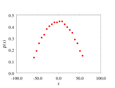
   Figure 1: The density distribution at $T=0$ for $N=800$ inside the parabolic potential well with $\alpha=10^{-3}f_{0}$. The simulation is identical to the one done by Andrade et al.. After the two extreme points on the left and on the right, the density is identically zero.

4. But again let us give a benefit of the doubt to Andrade et al. and ask the authors the following question. For $T=0$ it is very simple to find the position of mechanical equilibrium for N=1 or N=2,3,4,5…10 etc. We can also calculate the particle distribution in the thermodynamic limit, as was done in our Comment. In all these cases, the equilibrium is simply determined by the force balance. No statistics is involved. Our question is this: for exactly what value of N do authors expect that Tsallis entropy will start determining the particle distribution at T=0?

5. Now suppose that we raise the temperature. At some point the crystal will melt. However, the fluid state will still have strong correlations between individual particles. There is more than a hundred years of history, going all the way back to the pioneering works of Debye, Ornstein, Zernike, and Kirkwood on how the particle correlations can be calculated. There are thousands of liquid-state theorists who have dedicated their lives to understanding statistical mechanics of liquids — all this work simply ignored by Andrade et al.. In fact the correlations and their effects on the density distribution can be calculated in the framework of the usual Boltzmann-Gibbs statistical mechanics. There are theories, such as the Hypernetted Chain Equation, Roger-Young Equation, SCOZA, the Density Functional Theory, etc. which were derived to do exactly this. There is no reason to introduce any fitting parameters through Tsallis entropy. This does not lead to any new physical understanding, only to curve fitting. In fact, in their paper Andrade et al. did not provide any reason or indication why they believe that the standard Boltzmann-Gibbs statistical mechanics will not apply to the system of vertices studied by them.

6. In their Reply, Andrade et al. say that we did not question their non-linear Fokker-Planck equation (eq. 1 of Reply) on which are based all of their arguments. Indeed, because of the one page restriction we could not get into detailed discussion of the original paper, concentrating only on our exact solution for $T=0$. In fact, we do question the use of this non-linear Fokker-Planck equation to study the dynamics of interacting particles. This is an incorrect equation to use for this system. It is well known that the dynamics of interacting particles is governed by the self-consistent Nernst-Planck equation. Again, Andrade et al. got lucky because for the particles interacting through a modified Bessel function, the stationary solution (after adjusted with the fitting parameter as was done by Andrade et al.) is quite close to the correct solution of Nernst-Planck Equation. Thus, the asymptotic dynamics derived using the incorrect Fokker-Planck equation actually looks quite reasonable. In fact it is simple to see that eq. (1) used by Andrade et al. is incorrect. Using it Andrade et al. derived the unlucky eq. 13 of their PRL, from which all the incorrect discussion followed. From this equation Andrade et al. concluded that the stationary state for particles interacting by any short-range force is always parabolic – a Tsallis q-Gaussian of entropic index $\nu=2$. From our exact calculation, it is clear that the parabolic form is very special for the interaction potential of the modified Bessel form. Other potentials will not lead to the parabolic form. We should recall that Andrade et al. claim that their theory applies to particles interacting by an arbitrary short-range potential. As a simple demonstration that this is not true, we have simulated a 1d systems of particles interacting through a short range potential $V(x)=\frac{q^{2}}{2}e^{-x^{4}}$. In Fig.2, we see that once the system has relaxed to equilibrium, the distribution is not the inverse parabola, but a much more complicated function. One should also note the characteristic discontinuity in density, contradictory to Tsallis statistics. We conclude again that the non-linear Fokker-Planck equation of Andrade et al. can neither account for the stationary state nor for the dynamics of approach to equilibrium.

   

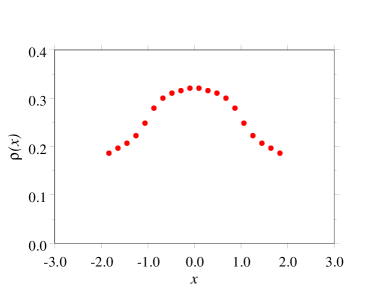
   Figure 2: The density distribution at $T=0$ for particles interacting by a short range potential $V(x)=\frac{q^{2}}{2}e^{-x^{4}}$ confined in a parabolic trap. To get better statistics and faster run time, we studied a 1d model, with $N=1000$, $\alpha=0.05$. Note, however, that because of the periodic boundary condition the model of Andrade et al. is also effectively 1d. Also note the discontinuous drop in density.

7. Andrade et al. have misinterpreted the interparticle correlations present in a finite system for existence of a new kind of entropy. The fact that the system studied by Andrade et al. is described by the usual Boltzmann-Gibbs statistical mechanics, follows simply from the study of velocity distribution in equilibrium. In Fig.3 we show a result of a microcanonical (constant energy) simulation. The system starts from an arbitrary initial condition and evolves in accordance with Newton’s equations of motion. After some time it relaxes to thermodynamic equilibrium. In Fig. 2 we plot the histogram of particle velocities together with the 2d Maxwell-Boltzmann distribution,

   $$n(v)=\frac{2v}{\langle v^{2}\rangle}e^{-\frac{v^{2}}{{\langle v^{2}\rangle}}}.$$

   We see a perfect agreement between the Boltzmann-Gibbs statistical mechanics and the simulations, without any adjustable parameters. In this example, the equilibrium temperature, $T=\langle v^{2}\rangle/2$, is very low $T=0.3$ and Andrade et al. claim that the system should be described by the Tsallis statistics. In fact we do not see any trace of q-exponentials at this or at any other temperature.

8. In their Reply Andrade et al. state that “neither the Maxwell-Boltzmann nor the Tsallis thermostatics are contrary to classical mechanics theory”. We respectfully disagree with this statement. Indeed the Boltzmann-Gibbs statistical mechanics is in full agreement with the classical mechanics. However, there is not a single classical system of particles interacting by a short-range potential (for long-range forces see LePa08 and the references therein) that evolves to “Tsallis” equilibrium. The model studied by Andrade et al. is precisely the case in point. Therefore, we stand by our original statement: “the density distribution of particles in contact with a reservoir at $T=0$ has nothing to do with the Tsallis statistics, and everything to do with the Newton’s Second Law.”

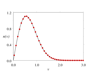
Figure 3: Velocity distribution. Points are from molecular-dynamics simulation, for exactly the system studied by Andrade et al., $N=800$, $L_{y}=20$, $\alpha=10^{-3}f_{0}$. Solid curve is the Maxwell-Boltzmann velocity distribution. There are no adjustable parameters. The temperature is $T=0.3$. At this temperature, Andrade et al. claim that the system is described by the Tsallis statistics. As is clear from the graph, we see no trace of Tsallis q-exponentials in the velocity distribution function.

This work was partially supported by the CNPq, INCT-FCx, and by the US-AFOSR under the grant FA9550-09-1-0283.

Yan Levin and Renato Pakter
Instituto de F sica, UFRGS
CP 15051, 91501-970, Porto Alegre, RS, Brazil

References

- (1) J. S. Andrade, Jr., et al, arXiv:1104.5036
- (2) Y. Levin and R. Pakter, arXiv:1104.0697
- (3) J. S. Andrade, Jr., et al., Phys. Rev. Lett. 105 260601 (2010).
- (4) Y. Levin, R. Pakter and T. N. Telles, Phys. Rev. Lett. 100, 040604 (2008); T.N. Teles, Y.Levin, R. Pakter, and F.B. Rizzato, J. Stat. Mech. P05007 (2010); R. Pakter and Y. Levin, arXiv:1012.0035 (2010)