Estimation in autoregressive model with measurement error

Abstract.

Consider an autoregressive model with measurement error: we observe $Z_{i}=X_{i}+\varepsilon_{i}$, where $X_{i}$ is a stationary solution of the autoregressive equation $X_{i}=f_{\theta^{0}}(X_{i-1})+\xi_{i}$. The regression function $f_{\theta^{0}}$ is known up to a finite dimensional parameter $\theta^{0}$. The distributions of $X_{0}$ and $\xi_{1}$ are unknown whereas the distribution of $\varepsilon_{0}$ is completely known. We want to estimate the parameter $\theta^{0}$ by using the observations $Z_{0},\ldots,Z_{n}$. We propose an estimation procedure based on a modified least square criterion. This procedure provides an asymptotically normal estimator $\hat{\theta}$ of $\theta^{0}$, for a large class of regression functions and various noise distributions.

(1) Laboratoire MAP5 UMR CNRS 8145, Université Paris Descartes, Sorbonne Paris Cité,
(2) Laboratoire Statistique et Génome UMR CNRS 8071- USC INRA, Université d’Évry Val d’Essonne

Keywords: autoregressive model, Markov chain, mixing, deconvolution, semi-parametric model.

AMS 2000 MSC: Primary 62J02, 62F12, Secondary 62G05, 62G20.

1. Introduction

We consider an autoregressive model with measurement error satisfying

(1.3) $$\left\{\begin{array}[]{ll}Z_{i}&=X_{i}+\varepsilon_{i},\\ X_{i}&=f_{\theta^{0}}(X_{i-1})+\xi_{i}\end{array}\right.$$

where one observes $Z_{0},\cdots,Z_{n}$ and the random variables $\xi_{i},X_{i},\varepsilon_{i}$ are unobserved. The regression function $f_{\theta^{0}}$ is known up to a finite dimensional parameter $\theta^{0}$, belonging to the interior $\Theta^{\circ}$ of a compact set $\Theta\subset\mathbb{R}^{d}$. The centered innovations $(\xi_{i})_{i\geq 1}$ and the errors $(\varepsilon_{i})_{i\geq 0}$ are independent and identically distributed (i.i.d.) random variables with finite variances $\mbox{Var}(\xi_{1})=\sigma_{\xi}^{2}$ and $\mbox{Var}(\varepsilon_{0})=\sigma_{\varepsilon}^{2}$. We assume that $\varepsilon_{0}$ admits a known density with respect to the Lebesgue measure, denoted by $f_{\varepsilon}$. Furthermore we assume that the random variables $X_{0}$, $(\xi_{i})_{i\geq 1}$ and $(\varepsilon_{i})_{i\geq 0}$ are independent. The distribution of $\xi_{1}$ is unknown and does not necessarily admit a density with respect to the Lebesgue measure. We assume that $(X_{i})_{i\geq 0}$ is strictly stationary, which means that the initial distribution of $X_{0}$ is an invariant distribution for the transition kernel of the homogeneous Markov chain $(X_{i})_{i\geq 0}$.

Our aim is to estimate $\theta^{0}$ for a large class of functions $f_{\theta}$, whatever the known error distribution, and without the knowledge of the $\xi_{i}$’s distribution. The distribution of the innovations being unknown, this model belongs to the family of semi-parametric models.

Previously known results

Several authors have considered the case where the function $f_{\theta}$ is linear (in both $\theta$ and $x$), see e.g. Andersen and Deistler ANDDEIS, Nowak Nowak, Chanda Chanda,Chanda96, Staudenmayer and Buonaccorsi StaudenmayerBuonaccorsi, and Costa et al. CostaAlpuim. We can note that, in this specific case, the model (1.3) is also an ARMA model (see Section 4.1.1 for further details). Consequently, all previously known estimation procedures for ARMA models can be applied here, without assuming that the error distribution is known.

For a general regression function, the model (1.3) is a Hidden Markov Model with possibly a non compact continuous state space, and with unknown innovation distribution. When the innovation distribution is known up to a finite dimensional parameter, the model (1.3) is fully parametric and various results are already stated. Among others, the parameters can be estimated by maximum likelihood, and consistency, asymptotic normality and efficiency have been proved. For further references on estimation in fully parametric Hidden Markov Models, we refer for instance to Leroux Leroux, Bickel et al. BickelRitovRyden, Jensen and Petersen JensenPetersen, Douc and Matias DoucMatias, Douc et al. DoucMoulinesRyden, Fuh Fuh2006, Genon-Catalot and Laredo VGCCL, Na et. al. Naetal, and Douc et al. DoucMoulinesOlssonvanHandel.

In this paper, we consider the case where the innovation distribution is unknown, and thus the model is not fully parametric. In this general context, there are few results. To our knowledge, the only paper which gives a consistent estimator is the paper by Comte and Taupin ComteTaupin2001. These authors propose an estimation procedure based on a modified least squares minimization. They give an upper bound for the rate of convergence of their estimator, that depends on the smoothness of the regression function and on the smoothness of $f_{\varepsilon}$. Those results are obtained by assuming that the distribution $P_{X}$ of $X_{0}$ admits a density $f_{X}$ with respect to the Lebesgue measure and that the stationary Markov chain $(X_{i})_{i\geq 0}$ is absolutely regular ($\beta$-mixing). The main drawback of their approach is that their estimation criterion is not explicit, hence the links between the convergence rate of their estimator and the smoothness of the regression function and of the error distribution are not explicit either. Consequently, Comte and Taupin ComteTaupin2001 are able to prove that their estimator achieves the parametric rate only for very few couples of regression functions/error distribution. Lastly their dependency conditions are quite restrictive, and the assumption that $X$ admits a density is not natural in this context.

Our results

In this paper, we propose a new estimation procedure which provides a consistent estimator with a parametric rate of convergence in a very general context. Our approach is based on the new contrast function

$$S_{\theta^{0},P_{X}}(\theta)=\mathbb{E}[(Z_{1}-f_{\theta}(X_{0}))^{2}\,w(X_{0})],$$

where $w$ is a weight function to be chosen and $\mathbb{E}$ is the expectation $\mathbb{E}_{\theta^{0},P_{X}}$. We assume that $w$ is such that $(wf_{\theta})^{*}/f_{\varepsilon}^{*}$ and $(wf_{\theta}^{2})^{*}/f_{\varepsilon}^{*}$ are integrable, where $\varphi^{*}$ is the Fourier transform of a function $\varphi$. We estimate $\theta^{0}$ by $\widehat{\theta}=\arg\min_{\theta\in\Theta}S_{n}(\theta),$ where

(1.4) $$S_{n}(\theta)=\frac{1}{2\pi n}\sum_{k=1}^{n}\mathbb{R}e\int\frac{\left(\big{(}Z_{k}-f_{\theta}\big{)}^{2}w\right)^{*}(t)\;e^{-itZ_{k-1}}}{f_{\varepsilon}^{*}(-t)}dt,$$

where $\mathbb{R}e(u)$ is the real part of $u$. Under general assumptions, we prove that the estimator defined $\widehat{\theta}$ is consistent. Moreover, we give some conditions under which the parametric rate of convergence as well as the asymptotic normality can be stated. Those results hold under weak dependency conditions as introduced in Dedecker and Prieur JDCPCoeff.

This procedure is clearly simpler than that of Comte and Taupin ComteTaupin2001. The resulting rate is more explicit and links directly the smoothness of the regression function to that of $f_{\varepsilon}$. Our new estimator is asymptotically Gaussian for a large class of regression functions, which is not the case in Comte and Taupin ComteTaupin2001.

The asymptotic properties of our estimator are illustrated through a simulation study. It confirms that our estimator performs well in various contexts, even in cases where the Markov chain $(X_{i})_{i\geq 0}$ is not $\beta$-mixing (and not even irreducible), when the ratio signal to noise is small or large, for various sample sizes, and for different types of error distribution. Our estimator always better performs than the so-called naive estimator (built by replacing the non-observed $X$ by $Z$ in the usual least squares criterion). Our estimation procedure depends on the choice of the weight function $w$. The influence of this weight function is also studied in the simulations.

Finally, we propose a more general estimator when it is not possible to find a weight function $w$ such that $(wf_{\theta})^{*}/f_{\varepsilon}^{*}$ and $(wf_{\theta}^{2})^{*}/f_{\varepsilon}^{*}$ are integrable. We establish a consistency result, and we give an upper bound for the quadratic risk, that relates the smoothness properties of the regression function to that of $f_{\varepsilon}$. These last results are proved under $\alpha$-mixing conditions.

The paper is organized as follows. In Section 2 we present our estimation procedure. The theoretical properties of the estimator are stated in Section 3. The simulations are presented in Section 4. In Section 5 we introduce a more general estimator and we describe its asymptotic behavior. The proofs are gathered in Appendix.

2. Estimation procedure

In order to define more rigorously the criterion presented in the introduction, we first give some preliminary notations and assumptions.

2.1. Notations

Let

$$\parallel\varphi\parallel_{1}=\int|\varphi(x)|dx,\;\parallel\varphi\parallel_{2}^{2}=\int\varphi^{2}(x)dx,\;\mbox{ and }\parallel\varphi\parallel_{\infty}=\sup_{x\in\mathbb{R}}|\varphi(x)|.$$

The convolution product of two square integrable functions $p$ and $q$ is denoted by $p\star q(z)=\int p(z-x)q(x)dx$. The Fourier transform $\varphi^{*}$ of a function $\varphi$ is defined by

$$\varphi^{*}(t)=\int e^{itx}\varphi(x)dx.$$

For $\theta\in\mathbb{R}^{d}$, let $\parallel\theta\parallel_{\ell^{2}}^{2}=\sum_{k=1}^{d}\theta_{k}^{2}$, and let $\theta^{\top}$ be the transpose matrix of $\theta$.

For a map $(\theta,u)\mapsto\varphi_{\theta}(u)$ from $\Theta\times\mathbb{R}$ to $\mathbb{R}$, the first and second derivatives with respect to $\theta$ are denoted by

$$\varphi^{(1)}_{\theta}(\cdot) = \left(\varphi_{\theta,j}^{(1)}(\cdot)\right)_{1\leq j\leq d},\ \mbox{ with }\varphi_{\theta,j}^{(1)}(\cdot)=\frac{\partial\varphi_{\theta}(\cdot)}{\partial\theta_{j}}\mbox{ for }j\in\{1,\cdots,d\}$$

$$\mbox{ and }\hskip 14.22636pt\varphi^{(2)}_{\theta}(\cdot) = \left(\varphi_{\theta,j,k}^{(2)}(\cdot)\right)_{1\leq j,k\leq d},\ \mbox{ with }\varphi_{\theta,j,k}^{(2)}(\cdot)=\frac{\partial^{2}\varphi_{\theta}(\cdot)}{\partial\theta_{j}\partial\theta_{k}},\mbox{ for }j,k\in\{1,\cdots,d\}.$$

From now, $\mathbb{P}$, $\mathbb{E}$ and Var denote respectively the probability $\mathbb{P}_{\theta^{0},P_{X}}$, the expected value $\mathbb{E}_{\theta^{0},P_{X}}$ and the variance $\mbox{Var}_{\theta^{0},P_{X}}$, when the underlying and unknown true parameters are $\theta^{0}$ and $P_{X}$.

2.2. Assumptions

We consider three types of assumptions.

$\bullet$ Smoothness and moment assumptions

($$\mathbf{A_{1}} \mbox{On $\Theta^{\circ}$, the function }\theta\mapsto f_{\theta}\mbox{ admits continuous derivatives with respect to }\theta\mbox{ up to the }$$)

$$\mbox{order 3}.$$

($$\mathbf{A_{2}} \mbox{On $\Theta^{\circ}$, the quantity }w(X_{0})(Z_{1}-f_{\theta}(X_{0}))^{2},\mbox{ and the absolute values of its derivatives}$$)

$$\mbox{with respect to }\theta\mbox{ up to order 2 have a finite expectation.}$$

$\bullet$ Identifiability assumptions

($$\mathbf{I1_{1}} \mbox{ The quantity }S_{\theta^{0},P_{X}}(\theta)=\mathbb{E}[(f_{\theta^{0}}(X)-f_{\theta}(X))^{2}w(X)]\mbox{ admits one unique minimum at}$$)

$$\theta=\theta^{0}.$$

($$\mathbf{I1_{2}} \mbox{ For all }\theta\in\Theta^{\circ},\mbox{ the matrix }S_{\theta^{0},P_{X}}^{(2)}(\theta)=\left(\frac{\partial^{2}S_{\theta^{0},P_{X}}(\theta)}{\partial\theta_{i}\partial\theta_{j}}\right)_{1\leq i,j\leq d}\mbox{ exists and the matrix }$$)

$$S^{(2)}_{\theta^{0},P_{X}}(\theta^{0})=2\,\mathbb{E}\left[w(X)\left(f^{(1)}_{\theta^{0}}(X)\right)\left(f^{(1)}_{\theta^{0}}(X)\right)^{\top}\right]\mbox{ is positive definite}.$$

$\bullet$ Assumptions on $f_{\varepsilon}$

($$\mathbf{N_{1}} \mbox{The density }f_{\varepsilon}\mbox{ belongs to }\mathbb{L}_{2}(\mathbb{R})\mbox{ and for all }x\in\mathbb{R},\;f_{\varepsilon}^{*}(x)\not=0.$$)

The assumption ($\mathbf{N_{1}}$) is quite usual when considering estimation in the convolution model. It ensures the existence of the estimation criterion.

2.3. Definition of the estimator

As already mentioned in the introduction, the starting point of our estimation procedure is to construct an estimator of the least square contrast

(2.5) $$S_{\theta^{0},P_{X}}(\theta)=\mathbb{E}[(Z_{1}-f_{\theta}(X_{0}))^{2}\,w(X_{0})],$$

based on the observations $(Z_{i})$ for $i=0,\ldots,n$.

We consider the following condition: there exists a weight function $w$ such that for all $\theta\in\Theta$,

($$\mathbf{C_{1}} \mbox{ The functions }(wf_{\theta})\mbox{ and }(wf_{\theta}^{2})\mbox{ belong to }\mathbb{L}_{1}(\mathbb{R}),\mbox{ and the functions }w^{*}/f_{\varepsilon}^{*}\,,(f_{\theta}w)^{*}/f_{\varepsilon}^{*}\,,$$)

$$\,(f_{\theta}^{2}w)^{*}/f_{\varepsilon}^{*}\mbox{ belong to }\mathbb{L}_{1}(\mathbb{R}).$$

Remark 2.1.

The first part of Condition ($\mathbf{C_{1}}$) is not restrictive. The second part can be heuristically expressed as “one can find a weight function $w$ such that $wf_{\theta}$ is smooth enough compared to $f_{\varepsilon}$”. For a large number of regression functions, such a weight function can be easily exhibited. Some practical choices are discussed in the simulation study (Section 4).

If ($\mathbf{C_{1}}$) holds, the expectations $\mathbb{E}(w(X))$, $\mathbb{E}(w(X)f_{\theta}(X))$ and $\mathbb{E}(w(X)f_{\theta}^{2}(X))$ can be easily estimated. Let us present the ideas of the estimation procedure. Let $\varphi$ be such that $\varphi$ and $\varphi^{*}/f_{\varepsilon}^{*}$ belong to $\mathbb{L}_{1}(\mathbb{R})$. For such a function, due to the independence between $\varepsilon_{0}$ and $X_{0}$ we have

$$\mathbb{E}[\varphi(X_{0})]=\mathbb{E}\left(\frac{1}{2\pi}\int\varphi^{*}(t)e^{-itX_{0}}dt\right)=\mathbb{E}\left(\frac{1}{2\pi}\int\frac{\varphi^{*}(t)e^{-itZ_{0}}}{f_{\varepsilon}^{*}(-t)}dt\right).$$

Hence, based on the observations $Z_{0},\cdots,Z_{n}$, $\mathbb{E}[\varphi(X_{0})]$ is estimated by

$$\frac{1}{2\pi}\mathbb{R}e\int\frac{\varphi^{*}(t)n^{-1}\sum_{j=1}^{n}e^{-itZ_{j}}}{f_{\varepsilon}^{*}(-t)}dt.$$

We then propose to estimate $S_{\theta^{0},P_{X}}(\theta)$ by the quantity $S_{n}(\theta)$ defined by

(2.6) $$S_{n}(\theta)=\frac{1}{2\pi n}\sum_{k=1}^{n}\mathbb{R}e\int\frac{\left(\big{(}Z_{k}-f_{\theta}\big{)}^{2}w\right)^{*}(t)\;e^{-itZ_{k-1}}}{f_{\varepsilon}^{*}(-t)}dt,$$

which satisfies

$$\mathbb{E}(S_{n}(\theta))=\mathbb{E}[(Z_{1}-f_{\theta}(X_{0}))^{2}w(X_{0})].$$

This criteria is minimum when $\theta=\theta^{0}$ under the identifiability assumption ($\mathbf{I1_{1}}$). Using this empirical criterion we propose to estimate $\theta^{0}$ by

(2.7) $$\widehat{\theta}=\arg\min_{\theta\in\Theta}S_{n}(\theta).$$

3. Asymptotic properties

In this section, we give some conditions under which our estimator is consistent and asymptotically normal.

3.1. Consistency of the estimator

The first result to mention is the consistency of our estimator. It holds under the following additional condition.

($$\mathbf{C_{2}} \mbox{ The functions }\sup_{\theta\in\Theta}\left|\big{(}f^{(1)}_{\theta,i}w\big{)}^{*}/f_{\varepsilon}^{*}\right|\mbox{ and }\sup_{\theta\in\Theta}\left|\big{(}f_{\theta}f^{(1)}_{\theta,i}w\big{)}^{*}/f_{\varepsilon}^{*}\right|\mbox{ belong to }\mathbb{L}_{1}(\mathbb{R})\mbox{ for any }$$)

$$i\in\{1,\ldots,d\}.$$

This condition is similar to ($\mathbf{C_{1}}$) for the first derivatives of $f_{\theta}$. Thus it is not more restrictive than ($\mathbf{C_{1}}$).

Theorem 3.1.

Consider Model (1.3) under the assumptions ($\mathbf{A_{1}}$)-($\mathbf{A_{2}}$), ($\mathbf{I1_{1}}$), ($\mathbf{I1_{2}}$), ($\mathbf{N_{1}}$), and the conditions ($\mathbf{C_{1}}$)-($\mathbf{C_{2}}$). Then $\widehat{\theta}$ defined by (2.7) converges in probability to $\theta^{0}$.

3.2. $\sqrt{n}$-consistency and asymptotic normality

To state the asymptotic normality of our estimator, we need to introduce some additional conditions.

($$\mathbf{C_{3}} \mbox{ the functions }\sup_{\theta\in\Theta}\left|\left(f^{(2)}_{\theta,i,j}w\right)^{*}/f_{\varepsilon}^{*}\right|\mbox{ and }\sup_{\theta\in\Theta}\left|\left(\frac{\partial^{2}}{\partial\theta_{i}\partial\theta_{j}}(f_{\theta}^{2}w)\right)^{*}/f_{\varepsilon}^{*}\right|\mbox{ belong to }\mathbb{L}_{1}(\mathbb{R})\mbox{ for}$$)

$$\mbox{ any }i,j\in\{1,\ldots,d\};$$

($$\mathbf{C_{4}} \mbox{ the functions }\sup_{\theta\in\Theta}\left|\left(\frac{\partial^{3}(f_{\theta}w)}{\partial\theta_{i}\partial\theta_{j}\partial\theta_{k}}\right)^{*}/f_{\varepsilon}^{*}\right|\mbox{ and }\sup_{\theta\in\Theta}\left|\left(\frac{\partial^{3}}{\partial\theta_{i}\partial\theta_{j}\partial\theta_{k}}(f_{\theta}^{2}w)\right)^{*}/f_{\varepsilon}^{*}\right|\mbox{ belong to }$$)

$$\mathbb{L}_{1}(\mathbb{R}),\mbox{ for }i,j,k\in\{1,\cdots,d\}.$$

($$\mathbf{C_{5}} \mbox{The integrals }\int|t(f_{\theta^{0}}w)^{*}(t)|dt\mbox{ and }\int|t(f_{\theta^{0}}f_{\theta^{0},k}^{(1)}w)^{*}(t)|dt\mbox{ are finite, for }k\in\{1,\cdots,d\}.$$)

The asymptotic properties of $\widehat{\theta}$, defined by (2.7), are stated under two different dependency conditions, which are presented below.

Definition 3.1.

Let $(\Omega,{\mathcal{A}},{\mathbb{P}})$ be a probability space. Let $Y$ be a random variable with values in a Banach space $({\mathbb{B}},\|\cdot\|_{\mathbb{B}})$. Denote by $\Lambda_{\kappa}({\mathbb{B}})$ the set of $\kappa$-Lipschitz functions, i.e. the functions $f$ from $({\mathbb{B}},\|\cdot\|_{\mathbb{B}})$ to ${\mathbb{R}}$ such that $|f(x)-f(y)|\leq\kappa\parallel x-y\parallel_{\mathbb{B}}$. Let ${\mathcal{M}}$ be a $\sigma$-algebra of ${\mathcal{A}}$. Let ${\mathbb{P}}_{Y|{\mathcal{M}}}$ be a conditional distribution of $Y$ given ${\mathcal{M}}$, $\mathbb{P}_{Y}$ the distribution of $Y$, and ${\mathcal{B}}({\mathbb{B}})$ the Borel $\sigma$-algebra on $({\mathbb{B}},\|\cdot\|_{\mathbb{B}})$. The dependence coefficients $\alpha$ and $\tau$ are defined by

$$\alpha({\mathcal{M}},\sigma(Y)) = \frac{1}{2}\sup_{A\in{\mathcal{B}}({\mathbb{B}})}{\mathbb{E}}(|{\mathbb{P}}_{Y|{\mathcal{M}}}(A)-{\mathbb{P}}_{Y}(A)|)\,,$$

$$\text{and if ${\mathbb{E}}(\|Y\|_{\mathbb{B}})<\infty$,}\quad\tau({\mathcal{M}},Y) = {\mathbb{E}}\Big{(}\sup_{f\in{\Lambda_{1}}({\mathbb{B}})}|{\mathbb{P}}_{Y|{\mathcal{M}}}(f)-{\mathbb{P}}_{Y}(f)|\Big{)}\,.$$

Let ${\bf X}=(X_{i})_{i\geq 0}$ be a strictly stationary Markov chain of real-valued random variables. On ${\mathbb{R}}^{2}$, we put the norm $\|x\|_{{\mathbb{R}}^{2}}=(|x_{1}|+|x_{2}|)/2$. For any integer $k\geq 0$, the coefficients $\alpha_{{\bf X}}(k)$ and $\tau_{{\bf X},2}(k)$ of the chain are defined by

$$\alpha_{{\bf X}}(k) = \alpha(\sigma(X_{0}),\sigma(X_{k}))$$

$$\text{and if ${\mathbb{E}}(|X_{0}|)<\infty$,}\quad\tau_{{\bf X},2}(k) = \sup\left\{\tau(\sigma(X_{0}),(X_{i_{1}},X_{i_{2}})),k\leq i_{1}\leq i_{2}\right\}.$$

Coefficient $\alpha({\mathcal{M}},\sigma(Y))$ is the usual strong mixing coefficient introduced by Rosenblatt Rosenblatt. Coefficient $\tau({\mathcal{M}},Y)$ has been introduced by Dedecker and Prieur JDCPCoeff. In Section A.2, we recall some conditions on $\xi_{0}$ and $f_{\theta^{0}}$ under which the Markov chain $(X_{i})_{i\geq 0}$ is $\alpha$-mixing or $\tau$-dependent and illustrate those conditions through some examples.

First we state the asymptotic normality of $\widehat{\theta}$ when the Markov chain $(X_{i})$ of Model (1.3) is $\alpha$-mixing.

Theorem 3.2.

Consider Model (1.3) under assumptions ($\mathbf{A_{1}}$), ($\mathbf{A_{2}}$), ($\mathbf{I1_{1}}$), ($\mathbf{I1_{2}}$), ($\mathbf{N_{1}}$), and conditions ($\mathbf{C_{1}}$)-($\mathbf{C_{4}}$). Let $Q_{|X_{1}|}$ be the inverse cadlag of the tail function $t\to{\mathbb{P}}(|X_{1}|>t)$. Assume that

(3.8) $$\sum_{k\geq 1}\int_{0}^{\alpha_{\bf X}(k)}Q_{|X_{1}|}^{2}(u)du<\infty\,.$$

Then $\widehat{\theta}$ defined by (2.7) is a $\sqrt{n}$-consistent estimator of $\theta^{0}$ which satisfies

$$\sqrt{n}(\widehat{\theta}-\theta^{0})\mathrel{\mathop{\kern 0.0pt\ \longrightarrow\ }\limits_{n\to\infty}^{{\mathcal{L}}}}\mathcal{N}(0,\Sigma_{1}),$$

where the covariance matrix $\Sigma_{1}$ is defined in equation (B.5).

Next, we give the corresponding result when the Markov chain $(X_{i})$ is $\tau$-dependent.

Theorem 3.3.

Consider Model (1.3) under assumptions ($\mathbf{A_{1}}$), ($\mathbf{A_{2}}$), ($\mathbf{I1_{1}}$), ($\mathbf{I1_{2}}$), ($\mathbf{N_{1}}$), and conditions ($\mathbf{C_{1}}$)-($\mathbf{C_{5}}$). Let $G(t)=t^{-1}{\mathbb{E}}(X_{1}^{2}{\mathbf{1}}_{X_{1}^{2}>t})$, and let $G^{-1}$ be the inverse cadlag of $G$. Assume that

(3.9) $$\quad\sum_{k>0}G^{-1}(\tau_{{\bf X},2}(k))\tau_{{\bf X},2}(k)<\infty\,.$$

Then $\widehat{\theta}$ defined by (2.7) is a $\sqrt{n}$-consistent estimator of $\theta^{0}$ which satisfies

$$\sqrt{n}(\widehat{\theta}-\theta^{0})\mathrel{\mathop{\kern 0.0pt\ \longrightarrow\ }\limits_{n\to\infty}^{{\mathcal{L}}}}\mathcal{N}(0,\Sigma_{1}),$$

where the covariance matrix $\Sigma_{1}$ is defined in equation (B.5).

Remark 3.1.

Let us give some conditions under which (3.8) or (3.9) are verified. Assume that ${\mathbb{E}}(|X_{0}|^{p})<\infty$ for some $p>2$. Then (3.8) is true provided that $\sum_{k>0}k^{2/(p-2)}\alpha_{\bf X}(k)<\infty$, and (3.9) is true provided that $\sum_{k>0}(\tau_{{\bf X},2}(k))^{(p-2)/p}<\infty$.

Note that those results do not require the Markov chain to be absolutely regular as it is the case in Comte and Taupin ComteTaupin2001. Consequently they apply to autoregressive models with weaker dependency conditions. Beside the dependency conditions, our estimation procedure allows to achieve the parametric rate for a larger class of regression functions than in Comte and Taupin ComteTaupin2001.

The conditions under which Theorems 3.2 and 3.3 hold are similar, except Condition ($\mathbf{C_{5}}$) which appears only in Theorem 3.3. This condition is just technical and not restrictive at all.

The choice of the weight function $w$ is crucial. Various weight functions can handle with Conditions $\mathbf{C_{1}}$-$\mathbf{C_{5}}$. The numerical properties of the resulting estimators will differ from one choice to another. This point is discussed on simulated data in the next section.

4. Simulation study

We investigate the properties of our estimator for different regression functions on simulated data. For each choice of regression function, we consider two error distributions: the Laplace distribution and the Gaussian distribution. When $\varepsilon_{1}$ has the Laplace distribution, its density and Fourier transform are

(4.10) $$f_{\varepsilon}(x)=\frac{1}{\sigma_{\varepsilon}\sqrt{2}}\exp\Big{(}-\frac{\sqrt{2}}{\sigma_{\varepsilon}}|x|\Big{)},\mbox{ and }f^{*}_{\varepsilon}(x)=\frac{1}{1+\sigma_{\varepsilon}^{2}x^{2}/2}.$$

Hence, $\varepsilon_{1}$ is centered with variance $\sigma_{\varepsilon}^{2}$.

When $\varepsilon_{1}$ is Gaussian, its density and Fourier transform are

(4.11) $$f_{\varepsilon}(x)=\frac{1}{\sigma_{\varepsilon}\sqrt{2\pi}}\exp\Big{(}-\frac{x^{2}}{2\sigma_{\varepsilon}^{2}}\Big{)},\mbox{ and }f^{*}_{\varepsilon}(x)=\exp(-\sigma_{\varepsilon}^{2}x^{2}/2).$$

Hence, $\varepsilon_{1}$ is centered with variance $\sigma_{\varepsilon}^{2}$.

For each of these error distributions, we consider the case of a linear regression function and of a Cauchy regression function. We start with the linear case.

4.1. Linear regression function

We consider the model (1.3) with $f_{\theta}(x)=ax+b$, where $|a|<1$ and $\theta=(a,b)^{T}$. In these simulations, we have chosen to illustrate the numerical properties of our estimator under the weakest of the dependency conditions, that is $\tau$-dependency. As it is recalled in Appendix A.2, when $f_{\theta^{0}}$ is linear with $|a|<1$, if $\xi_{0}$ has a density bounded from below in a neighborhood of the origin, then the Markov chain $(X_{i})_{i\geq 0}$ is $\alpha$-mixing. When $\xi_{0}$ does not have a density, then the chain may not be $\alpha$-mixing (and not even irreducible), but it is always $\tau$-dependent.

Here, we consider the case where the innovation distribution is discrete, in such a way that the stationary Markov Chain is $\tau$-dependent but not $\alpha$-mixing. We also consider two distinct values of $\theta_{0}$. For the first value, the stationary distribution of $X_{i}$ is absolutely continuous with respect to the Lebesgue measure. For the second value, the stationary distribution is singular with respect to the Lebesgue measure. In both cases Theorem 3.3 applies, and the estimator $\hat{\theta}$ is asymptotically normal.

$\bullet$ Case A (absolutely continuous stationary distribution). We focus on the case where the true parameter is $\theta^{0}=(1/2,1/4)^{T}$, $X_{0}$ is uniformly distributed over $[0,1]$, and $(\xi_{i})_{i\geq 1}$ is a sequence of i.i.d. random variables, independent of $X_{0}$ and such that ${\mathbb{P}}(\xi_{1}=-1/4)={\mathbb{P}}(\xi_{1}=1/4)=1/2$. Then the Markov chain defined for $i>0$ by

(4.12) $$X_{i}=\frac{1}{4}+\frac{1}{2}X_{i-1}+\xi_{i}$$

is strictly stationary, the stationary distribution being the uniform distribution over $[0,1]$, and consequently $\sigma_{X_{0}}^{2}=1/12$. This chain is non-irreducible, and the dependency coefficients are such that $\alpha_{\bf X}(k)=1/4$ (see for instance Bradley Bradley86, p. 180) and $\tau_{{\bf X},2}(k)=O(2^{-k})$. Thus the Markov chain is not $\alpha$-mixing, but it is $\tau$-dependent. For the simulation, we start with $X_{0}$ uniformly distributed over $[0,1]$, so the simulated chain is stationary.

$\bullet$ Case B (singular stationary distribution). We consider the case where the true parameter is $\theta^{0}=(1/3,1/3)^{T}$, $X_{0}$ is uniformly distributed over the Cantor set, and $(\xi_{i})_{i\geq 1}$ is a sequence of i.i.d. random variables, independent of $X_{0}$ and such that ${\mathbb{P}}(\xi_{1}=-1/3)={\mathbb{P}}(\xi_{1}=1/3)=1/2$. Then the Markov chain defined for $i>0$ by

(4.13) $$X_{i}=\frac{1}{3}+\frac{1}{3}X_{i-1}+\xi_{i}$$

is strictly stationary, the stationary distribution being the uniform distribution over the Cantor set, and consequently $\sigma_{X}^{2}=1/8$. This chain is non-irreducible, and the dependency coefficients satisfy $\alpha_{\bf X}(k)=1/4$ and $\tau_{{\bf X},2}(k)=O(3^{-k})$. Thus the Markov chain is not $\alpha$-mixing, but is $\tau$-dependent. For the simulation, we start with $X_{0}$ uniformly distributed over $[0,1]$, and we consider that the chain is close to the stationary chain after 1000 iterations. We then set $X_{i}=X_{i+1000}$.

In these two cases, we can find a weight function $w$ satisfying the conditions ($\mathbf{C_{1}}$)-($\mathbf{C_{5}}$). We first give the detailed expression of the estimator for two choices of weight functions $w$. Then we recall the classic estimator when $X$ is directly observed, the ARMA estimator, and the so-called naive estimator.

4.1.1. Expression of the estimator.

We consider the two following weight functions $w$

(4.14) $$w(x)=N(x)=\exp\{-x^{2}/(4\sigma_{\varepsilon}^{2})\}\ \mbox{ and }\ w(x)=SC(x)=\frac{1}{2\pi}\Big{(}\frac{2*\sin(x)}{x}\Big{)}^{4}.$$

These choices of weight ensure that Conditions ($\mathbf{C_{1}}$)-($\mathbf{C_{5}}$) hold and that the two estimators, denoted by $\widehat{\theta}_{N}$ and $\widehat{\theta}_{SC}$ respectively, converge to $\theta^{0}$ with the parametric rate of convergence. There are two main differences between these two weight functions. First, $N$ depends on the variance error $\sigma_{\varepsilon}^{2}$. Hence the estimator should be adaptive to the noise level. On the contrary, it may be sensitive to very small error variance as it appears in the simulations (see Figure 1). Second, $SC$ has strong smoothness properties since its Fourier transform is compactly supported.

The two associated estimators are based on the calculation of $S_{n}(\theta)$, which can be written as

$$S_{n}(\theta)=\frac{1}{n}\sum_{k=1}^{n}[(Z_{k}^{2}+b^{2}-2Z_{k}b)I_{0}(Z_{k-1})+a^{2}I_{2}(Z_{k-1})-2a(Z_{k}-b)I_{1}(Z_{k-1})],$$

with

(4.15) $$I_{j}(Z)=\frac{1}{2\pi}\mathbb{R}e\int(p_{j}w)^{*}(u)\frac{e^{-iuZ}}{f_{\varepsilon}^{*}(-u)}du,$$

where $p_{j}(x)=x^{j}$ for $j=0,1,2$, $w$ being either $w=N$ or $w=SC$. With the above notations, $\widehat{\theta}=(\widehat{a},\widehat{b})^{T}$ satisfies

(4.16) $$\widehat{a} = \frac{\sum_{k=1}^{n}Z_{k}I_{1}(Z_{k-1})\sum_{k=1}^{n}I_{0}(Z_{k-1})-\sum_{k=1}^{n}Z_{k}I_{0}(Z_{k-1})\sum_{k=1}^{n}I_{1}(Z_{k-1})}{\sum_{k=1}^{n}I_{2}(Z_{k-1})\sum_{k=1}^{n}I_{0}(Z_{k-1})-\big{(}\sum_{k=1}^{n}I_{1}(Z_{k-1})\big{)}^{2}},$$

(4.17) $$\widehat{b} = \frac{\sum_{k=1}^{n}Z_{k}I_{0}(Z_{k-1})}{\sum_{k=1}^{n}I_{0}(Z_{k-1})}-\widehat{a}\frac{\sum_{k=1}^{n}I_{1}(Z_{k-1})}{\sum_{k=1}^{n}I_{0}(Z_{k-1})}.$$

We now compute $I_{j}(Z)$ for $j=0,1,2$ and the two weight functions. In the following we respectively denote $I_{j,N}(Z)$ and $I_{j,SC}(Z)$ the previous integrals when the weight function is either $w=N$ or $w=SC$.

We start with $w=N$ and give the details of the calculations for the two error distributions (Laplace and Gaussian), which are explicit. Then, with the weight function $w=SC$, we present the calculations, which are not explicit whatever the error distribution $f_{\varepsilon}$.

$\bullet$ When $w=N$, Fourier calculations provide that

$$N^{*}(t) = \sqrt{2\pi}\sqrt{2\sigma_{\varepsilon}^{2}}\exp(-\sigma_{\varepsilon}^{2}t^{2})$$

$$(Np_{1})^{*}(t) = \sqrt{2\pi}\sqrt{2\sigma_{\varepsilon}^{2}}\exp(-\sigma_{\varepsilon}^{2}t^{2})\big{(}-2\sigma_{\varepsilon}^{2}t/i\big{)},$$

$$(Np_{2})^{*}(t) = -\sqrt{2\pi}\sqrt{2\sigma_{\varepsilon}^{2}}\exp(-\sigma_{\varepsilon}^{2}t^{2})\big{(}-2\sigma_{\varepsilon}^{2}+4\sigma_{\varepsilon}^{4}t^{2}\big{)}.$$

It follows that

$$I_{0,N}(Z) = \frac{1}{2\pi}\mathbb{R}e\int\sqrt{2\pi}\sqrt{2\sigma_{\varepsilon}^{2}}\exp(-\sigma_{\varepsilon}^{2}t^{2})\frac{e^{-itZ}}{f_{\varepsilon}^{*}(-t)}dt,$$

$$I_{1,N}(Z) = \frac{1}{2\pi}\mathbb{R}e\int\sqrt{2\pi}\sqrt{2\sigma_{\varepsilon}^{2}}\exp(-\sigma_{\varepsilon}^{2}t^{2})\big{(}-2\sigma_{\varepsilon}^{2}t/i\big{)}\frac{e^{-itZ}}{f_{\varepsilon}^{*}(-t)}dt,$$

$$I_{2,N}(Z) = \frac{1}{2\pi}\mathbb{R}e\int\sqrt{2\pi}\sqrt{2\sigma_{\varepsilon}^{2}}\exp(-\sigma_{\varepsilon}^{2}t^{2})\big{(}2\sigma_{\varepsilon}^{2}-4\sigma_{\varepsilon}^{4}t^{2}\big{)}\frac{e^{-itZ}}{f_{\varepsilon}^{*}(-t)}dt.$$

If $f_{\varepsilon}$ is the Laplace distribution (4.10), replacing $f_{\varepsilon}^{*}$ by its expression we get

$$I_{0,N}(Z) = e^{-Z^{2}/(4\sigma_{\varepsilon}^{2})}-\frac{\sigma_{\varepsilon}^{2}}{2}\frac{\partial^{2}}{\partial Z^{2}}N(Z)=\left[5/4-Z^{2}/(8\sigma_{\varepsilon}^{2})\right]e^{-Z^{2}/(4\sigma_{\varepsilon}^{2})},$$

$$I_{1,N}(Z)=\left[7Z/4-Z^{3}/(8\sigma_{\varepsilon}^{2})\right]e^{-Z^{2}/(4\sigma_{\varepsilon}^{2})},I_{2,N}(Z)=\left[-\sigma_{\varepsilon}^{2}+9Z^{2}/4-Z^{4}/(8\sigma_{\varepsilon}^{2})\right]e^{-Z^{2}/(4\sigma_{\varepsilon}^{2})}.$$

If $f_{\varepsilon}$ is the Gaussian distribution (4.11), replacing $f_{\varepsilon}^{*}$ by its expression we obtain

$$I_{0,N}(Z)=\sqrt{2}e^{-Z^{2}/(2\sigma_{\varepsilon}^{2})},\quad I_{1,N}(Z)=2\sqrt{2}Ze^{-Z^{2}/(2\sigma_{\varepsilon}^{2})}\quad\mbox{and}\quad~{}~{}~{}I_{2,N}(Z)=\sqrt{2}(4Z^{2}-2\sigma_{\varepsilon}^{2})e^{-Z^{2}/(2\sigma_{\varepsilon}^{2})}.$$

Hence we deduce the expression of $\widehat{a}_{N}$ and $\widehat{b}_{N}$ by applying (4.16) and (4.17).

$\bullet$When $w=SC$, Fourier calculations provide that

$$SC^{*}(t) = {{{1}}{\mathrm{I}}}_{[-4,-2]}(t)(t^{3}/6+2t^{2}+8t+32/3)+{{{1}}{\mathrm{I}}}_{[-2,0]}(t)(-t^{3}/2-2t^{2}+16/3)$$

$$+{{{1}}{\mathrm{I}}}_{[2,4]}(t)(-t^{3}/6+2t^{2}-8t+32/3)+{{{1}}{\mathrm{I}}}_{[0,2]}(t)(t^{3}/2-2t^{2}+16/3)$$

$$(SCp_{1})^{*}(t) = \frac{\partial}{\partial t}SC^{*}(t)/i\mbox{ and }(SCp_{2})^{*}(t)=\frac{\partial^{2}}{\partial t^{2}}SC^{*}(t)/(i^{2}).$$

The integrals $I_{j,SC}(Z)$, defined for $j=0,1,2$ by

(4.18) $$I_{j,SC}(Z)=\frac{1}{2\pi}\mathbb{R}e\int(SCp_{j})^{*}(t)\frac{e^{-itZ}}{f_{\varepsilon}^{*}(-t)}dt,$$

have no explicit form, whatever the error distribution $f_{\varepsilon}$. It has to be numerically computed, using the IFFT Matlab function. More precisely, we consider a finite Fourier series approximation of ${(SCp_{j})^{*}(t)}/{f_{\varepsilon}^{*}(t)}$ whose Fourier transfom is calculated using IFFT Matlab function. The result is taken as an approximation of $I_{j,SC}(Z)$. Finally we deduce the expression of $\widehat{a}_{SC}$ and $\widehat{b}_{SC}$ by applying (4.16) and (4.17).

4.1.2. Comparison with classical estimators

We compare the two estimators $\widehat{\theta}_{N}$ and $\widehat{\theta}_{SC}$ with three classical estimators, the usual least square estimator when there is no observation noise, the ARMA estimator, and the so-called naive estimator.

$\bullet$ Estimator without noise. In the case where $\varepsilon_{i}=0$, that is $(X_{0},\ldots,X_{n})$ is observed without error, the parameters can be easily estimated by the usual least square estimators

$$\widehat{a}_{X}=\frac{n\sum_{i=1}^{n}X_{i}X_{i-1}-\sum_{i=1}^{n}X_{i}\sum_{i=1}^{n}X_{i-1}}{n\sum_{i=1}^{n}X_{i-1}^{2}-(\sum_{i=1}^{n}X_{i-1})^{2}}\quad\mbox{and}\quad\widehat{b}_{X}=\frac{1}{n}\Big{(}\sum_{i=1}^{n}X_{i}\Big{)}-\widehat{a}_{X}\frac{1}{n}\Big{(}\sum_{i=1}^{n}X_{i-1}\Big{)}\,.$$

$\bullet$ ARMA estimator. When the regression function is linear, the model may be written as

$$Z_{i}-aZ_{i-1}-b=\xi_{i}+\varepsilon_{i}-a\varepsilon_{i-1}\,.$$

The auto-covariance function $\gamma_{Y}$ of the stationary sequence $Y_{i}=\xi_{i}+\varepsilon_{i}-a\varepsilon_{i-1}$ is given by

$$\gamma_{Y}(0)=(1+a^{2})\sigma_{\varepsilon}^{2}+\sigma_{\xi}^{2},\quad\gamma_{Y}(1)=-a\sigma_{\varepsilon}^{2},\quad\text{and $\gamma_{Y}(k)=0$ for $k>1$}.$$

It follows that $Y_{i}$ is an MA(1) process, which may be written as

$$Y_{i}=\eta_{i}-\beta\eta_{i-1},$$

where $\eta_{i}$ is the innovation, and $|\beta|<1$ (note that $|\beta|\neq 1$ because $\gamma_{Y}(0)-2|\gamma_{Y}(1)|>0$). Moreover, one can give the explicit expression of $\beta$ and $\sigma_{\eta}^{2}$ in terms of $a,\sigma_{\xi}^{2}$ and $\sigma_{\varepsilon}^{2}$. It follows that, if $|a|<1$, $(Z_{i})_{i\geq 0}$ is the causal invertible ARMA(1,1) process

(4.19) $$Z_{i}-aZ_{i-1}=b+\eta_{i}-\beta\eta_{i-1}.$$

Note that $a\neq\beta$ except if $a=0$. Hence, if $|a|<1$ and $a\neq 0$, one can estimate the parameters $(a,b,\beta)$ by maximizing the so-called Gaussian likelihood. These estimators are consistent and asymptotically Gaussian. Moreover they are efficient when both the innovations and the errors $\varepsilon$ are Gaussian (see Hannan Hannan73 or Brockwell and Davis BrockwellDavis). Note that this well-known approach does not require the knowledge of the error distribution, but of course it works only in the particular case where the regression function $f_{\theta}$ is linear. For the computation of the ARMA estimator we use the function arma from the R tseries package (see Trapletti and Hornik Rtseries). The resulting estimators are denoted by $\widehat{a}_{arma}$ and $\widehat{b}_{arma}$.

$\bullet$ Naive estimator. The naive estimator is constructed by replacing the unobserved $X_{i}$ by the observation $Z_{i}$ in the expression of $\widehat{a}_{X}$ and $\widehat{b}_{X}$:

$$\widehat{a}_{naive}=\frac{n\sum_{i=1}^{n}Z_{i}Z_{i-1}-\sum_{i=1}^{n}Z_{i}\sum_{i=1}^{n}Z_{i-1}}{n\sum_{i=1}^{n}Z_{i-1}^{2}-(\sum_{i=1}^{n}Z_{i-1})^{2}}\quad\mbox{and}\quad\widehat{b}_{naive}=\frac{1}{n}\Big{(}\sum_{i=1}^{n}Z_{i}\Big{)}-\widehat{a}_{naive}\frac{1}{n}\Big{(}\sum_{i=1}^{n}Z_{i-1}\Big{)}\,.$$

Classical results show that $\widehat{\theta}_{naive}$ is an asymptotically biased estimator of $\theta^{0}$, which is confirmed by the simulation study.

4.1.3. Simulation results

For each error distribution, we simulate 100 samples with size $n$, $n=500$, $5000$ and $10000$. We consider different values of $\sigma_{\varepsilon}$ such that the ratio signal to noise $s2n=\sigma_{\varepsilon}^{2}/\mbox{Var}(X)$ is $0.5,1.5$ or $3$. The comparison of the five estimators is based on the bias, the Mean Squared Error (MSE), and the box plots. If $\widehat{\theta}(k)$ denotes the value of the estimation for the $k$-th sample, the MSE is evaluated by the empirical mean over the 100 samples:

$$MSE(\widehat{\theta})=\frac{1}{100}\sum_{k=1}^{100}(\widehat{\theta}(k)-\theta^{0})^{2}.$$

Results are presented in Figures 1-2 and Tables 1-4.

	ratio		Estimator
n	s2n		$\widehat{\theta}_{arma}(MSE)$	$\widehat{\theta}_{N}(MSE)$	$\widehat{\theta}_{SC}(MSE)$	$\widehat{\theta}_{X}(MSE)$	$\widehat{\theta}_{naive}(MSE)$
$1000$	0.5	a	0.487 (0.008)	0.459 (0.020)	0.489 (0.002)	0.493 (0.001)	0.328 (0.030)
		b	0.257 (0.002)	0.262 (0.002)	0.255 (0.001)	0.253 (0.001)	0.336 (0.008)
	1.5	a	0.494 (0.015)	0.488 (0.013)	0.492 (0.006)	0.501 (0.001)	0.198 (0.092)
		b	0.251 (0.004)	0.253 (0.002)	0.253 (0.002)	0.249 (0.001)	0.399 (0.023)
	3	a	0.461 (0.044)	0.502 (0.029)	0.503 (0.026)	0.493 (0.001)	0.121 (0.145)
		b	0.270 (0.012)	0.249 (0.001)	0.249 (0.001)	0.253 (0.001)	0.440 (0.037)
$5000$	0.5	a	0.497 (0.001)	0.499 (0.004)	0.499 (0.001)	0.499 (0.001)	0.332 (0.028)
		b	0.252 (0.001)	0.251 (0.001)	0.251 (0.001)	0.251 (0.001)	0.334 (0.007)
	1.5	a	0.498 (0.003)	0.508 (0.003)	0.503 (0.002)	0.499 (0.001)	0.199 (0.091)
		b	0.250 (0.001)	0.247 (0.001)	0.248 (0.001)	0.250 (0.001)	0.399 (0.022)
	3	a	0.487 (0.008)	0.492 (0.004)	0.495 (0.004)	0.500 (0.001)	0.123 (0.143)
		b	0.256 (0.002)	0.253 (0.001)	0.252 (0.001)	0.250 (0.001)	0.437 (0.035)
$10000$	0.5	a	0.496 (0.001)	0.501 (0.002)	0.500 (0.001)	0.499 (0.001)	0.334 (0.028)
		b	0.252 (0.001)	0.250 (0.001)	0.250 (0.001)	0.250 (0.001)	0.333 (0.007)
	1.5	a	0.504 (0.002)	0.500 (0.001)	0.501 (0.001)	0.500 (0.001)	0.200 (0.090)
		b	0.248 (0.001)	0.250 (0.001)	0.250 (0.001)	0.250 (0.001)	0.401 (0.023)
	3	a	0.493 (0.003)	0.499 (0.001)	0.499 (0.002)	0.498 (0.001)	0.124 (0.142)
		b	0.254 (0.001)	0.250 (0.001)	0.250 (0.001)	0.251 (0.001)	0.438 (0.036)

Table 1. Estimation results for Linear Case A, Laplace error. Mean estimated values of the five estimators $\widehat{\theta}_{arma}$, $\widehat{\theta}_{N}$, $\widehat{\theta}_{SC}$, $\widehat{\theta}_{X}$ and $\widehat{\theta}_{naive}$ are presented for various values of $n$ ($1000$, 5000 or 10000) and s2n (0.5, 1.5, 3). True values are $a^{0}=1/2$, $b^{0}=1/4$. MSEs are given in brackets.

	ratio		Estimator
n	s2n		$\widehat{\theta}_{arma}(MSE)$	$\widehat{\theta}_{N}(MSE)$	$\widehat{\theta}_{SC}(MSE)$	$\widehat{\theta}_{X}(MSE)$	$\widehat{\theta}_{naive}(MSE)$
$1000$	0.5	a	0.483 (0.006)	0.539 (0.039)	0.496 (0.002)	0.495 (0.001)	0.331 (0.030)
		b	0.259 (0.002)	0.243 (0.003)	0.253 (0.001)	0.253 (0.001)	0.336 (0.008)
	1.5	a	0.497 (0.021)	0.516 (0.027)	0.507 (0.009)	0.499 (0.001)	0.200 (0.091)
		b	0.251 (0.005)	0.243 (0.005)	0.246 (0.002)	0.249 (0.001)	0.399 (0.023)
	3	a	0.456 (0.031)	0.521 (0.082)	0.481 (0.030)	0.501 (0.001)	0.120 (0.145)
		b	0.272 (0.008)	0.244 (0.016)	0.260 (0.007)	0.250 (0.001)	0.441 (0.037)
$5000$	0.5	a	0.497 (0.001)	0.492 (0.006)	0.499 (0.001)	0.498 (0.001)	0.333 (0.028)
		b	0.251 (0.001)	0.252 (0.001)	0.250 (0.001)	0.250 (0.001)	0.333 (0.007)
	1.5	a	0.490 (0.002)	0.510 (0.006)	0.502 (0.001)	0.499 (0.001)	0.120 (0.090)
		b	0.254 (0.001)	0.245 (0.001)	0.248 (0.001)	0.250 (0.001)	0.399 (0.022)
	3	a	0.471 (0.010)	0.512 (0.008)	0.503 (0.005)	0.498 (0.001)	0.124 (0.141)
		b	0.263 (0.002)	0.245 (0.002)	0.249 (0.001)	0.251 (0.001)	0.437 (0.035)
$10000$	0.5	a	0.504 (0.006)	0.500 (0.003)	0.498 (0.001)	0.499 (0.001)	0.331 (0.028)
		b	0.249 (0.001)	0.250 (0.001)	0.251 (0.001)	0.251 (0.001)	0.335 (0.007)
	1.5	a	0.495 (0.002)	0.501 (0.002)	0.499 (0.001)	0.501 (0.001)	0.200 (0.090)
		b	0.253 (0.001)	0.250 (0.001)	0.251 (0.001)	0.250 (0.001)	0.401 (0.023)
	3	a	0.492 (0.004)	0.498 (0.004)	0.500 (0.003)	0.500 (0.001)	0.126 (0.140)
		b	0.254 (0.001)	0.251 (0.001)	0.251 (0.001)	0.250 (0.001)	0.437 (0.009)

Table 2. Estimation results for Linear Case A, Gaussian error. Mean estimated values of the five estimators $\widehat{\theta}_{arma}$, $\widehat{\theta}_{N}$, $\widehat{\theta}_{SC}$, $\widehat{\theta}_{X}$ and $\widehat{\theta}_{naive}$ are presented for various values of $n$ ($1000$, 5000 or 10000) and s2n (0.5, 1.5, 3). True values are $a^{0}=1/2$, $b^{0}=1/4$. MSEs are given in brackets.

	ratio		Estimator
n	s2n		$\widehat{\theta}_{arma}(MSE)$	$\widehat{\theta}_{N}(MSE)$	$\widehat{\theta}_{SC}(MSE)$	$\widehat{\theta}_{X}(MSE)$	$\widehat{\theta}_{naive}(MSE)$
$1000$	0.5	a	0.288 (0.021)	0.341 (0.013)	0.330 (0.002)	0.326 (0.001)	0.217 (0.015)
		b	0.354 (0.005)	0.331 (0.001)	0.333 (0.001)	0.335 (0.001)	0.389 (0.004)
	1.5	a	0.298 (0.050)	0.332 (0.009)	0.335 (0.007)	0.330 (0.001)	0.136 (0.040)
		b	0.349 (0.012)	0.331 (0.002)	0.329 (0.002)	0.335 (0.001)	0.429 (0.010)
	3	a	0.240 (0.127)	0.343 (0.017)	0.343 (0.018)	0.330 (0.001)	0.084 (0.063)
		b	0.385 (0.033)	0.333 (0.003)	0.333 (0.003)	0.338 (0.001)	0.465 (0.018)
$5000$	0.5	a	0.333 (0.004)	0.335 (0.003)	0.335 (0.001)	0.333 (0.001)	0.223 (0.012)
		b	0.333 (0.001)	0.332 (0.001)	0.332 (0.001)	0.334 (0.001)	0.388 (0.003)
	1.5	a	0.331 (0.011)	0.328 (0.002)	0.334 (0.001)	0.334 (0.001)	0.433 (0.041)
		b	0.334 (0.003)	0.334 (0.001)	0.329 (0.001)	0.332 (0.001)	0.132 (0.010)
	3	a	0.290 (0.030)	0.329 (0.003)	0.329 (0.004)	0.333 (0.001)	0.083 (0.063)
		b	0.355 (0.008)	0.335 (0.008)	0.335 (0.008)	0.334 (0.001)	0.459 (0.016)
$10000$	0.5	a	0.337 (0.002)	0.335 (0.002)	0.334 (0.001)	0.334 (0.001)	0.222 (0.012)
		b	0.331 (0.001)	0.332 (0.001)	0.332 (0.001)	0.332 (0.001)	0.388 (0.003)
	1.5	a	0.322 (0.006)	0.336 (0.001)	0.336 (0.001)	0.334 (0.001)	0.134 (0.040)
		b	0.339 (0.002)	0.332 (0.001)	0.332 (0.001)	0.333 (0.001)	0.433 (0.010)
	3	a	0.329 (0.010)	0.336 (0.002)	0.336 (0.002)	0.334 (0.001)	0.083 (0.063)
		b	0.335 (0.002)	0.332 (0.001)	0.332 (0.001)	0.332 (0.001)	0.457 (0.015)

Table 3. Estimation results for Linear Case B, Laplace error. Mean estimated values of the five estimators $\widehat{\theta}_{arma}$, $\widehat{\theta}_{N}$, $\widehat{\theta}_{SC}$, $\widehat{\theta}_{X}$ and $\widehat{\theta}_{naive}$ are presented for various values of $n$ ($1000$, 5000 or 10000) and s2n (0.5, 1.5, 3). True values are $a^{0}=1/3$, $b^{0}=1/3$. MSEs are given in brackets.

	ratio		Estimator
n	s2n		$\widehat{\theta}_{arma}(MSE)$	$\widehat{\theta}_{N}(MSE)$	$\widehat{\theta}_{SC}(MSE)$	$\widehat{\theta}_{X}(MSE)$	$\widehat{\theta}_{naive}(MSE)$
$1000$	0.5	a	0.327 (0.016)	0.349 (0.035)	0.330 (0.003)	0.326 (0.001)	0.218 (0.014)
		b	0.338 (0.004)	0.332 (0.002)	0.336 (0.001)	0.337 (0.001)	0.392 (0.004)
	1.5	a	0.290 (0.061)	0.355 (0.021)	0.345 (0.008)	0.332 (0.001)	0.133 (0.041)
		b	0.353 (0.015)	0.324 (0.004)	0.328 (0.002)	0.333 (0.001)	0.432 (0.010)
	3	a	0.234 (0.153)	0.329 (0.049)	0.329 (0.051)	0.326 (0.001)	0.077 (0.067)
		b	0.383 (0.040)	0.337 (0.010)	0.337 (0.010)	0.337 (0.001)	0.461 (0.017)
$5000$	0.5	a	0.329 (0.004)	0.341 (0.005)	0.333 (0.001)	0.332 (0.001)	0.220 (0.013)
		b	0.335 (0.001)	0.332 (0.001)	0.334 (0.001)	0.334 (0.001)	0.399 (0.003)
	1.5	a	0.329 (0.009)	0.331 (0.003)	0.332 (0.002)	0.333 (0.001)	0.132 (0.041)
		b	0.335 (0.002)	0.334 (0.001)	0.333 (0.001)	0.333 (0.001)	0.433 (0.010)
	3	a	0.315 (0.022)	0.348 (0.008)	0.348 (0.008)	0.334 (0.001)	0.084 (0.062)
		b	0.343 (0.006)	0.327 (0.002)	0.328 (0.002)	0.332 (0.001)	0.459 (0.016)
$10000$	0.5	a	0.330 (0.002)	0.333 (0.003)	0.333 (0.001)	0.332 (0.001)	0.221 (0.013)
		b	0.335 (0.001)	0.333 (0.001)	0.333 (0.001)	0.334 (0.001)	0.389 (0.003)
	1.5	a	0.328 (0.006)	0.336 (0.002)	0.334 (0.001)	0.333 (0.001)	0.132 (0.041)
		b	0.336 (0.002)	0.333 (0.001)	0.334 (0.001)	0.334 (0.001)	0.435 (0.010)
	3	a	0.312 (0.014)	0.334 (0.004)	0.334 (0.004)	0.333 (0.001)	0.083 (0.063)
		b	0.344 (0.003)	0.333 (0.001)	0.333 (0.001)	0.333 (0.001)	0.458 (0.016)

Table 4. Estimation results for Linear Case B, Gaussian error. Mean estimated values of the five estimators $\widehat{\theta}_{arma}$, $\widehat{\theta}_{N}$, $\widehat{\theta}_{SC}$, $\widehat{\theta}_{X}$ and $\widehat{\theta}_{naive}$ are presented for various values of $n$ ($1000$, 5000 or 10000) and s2n (0.5, 1.5, 3). True values are $a^{0}=1/3$, $b^{0}=1/3$. MSEs are given in brackets.

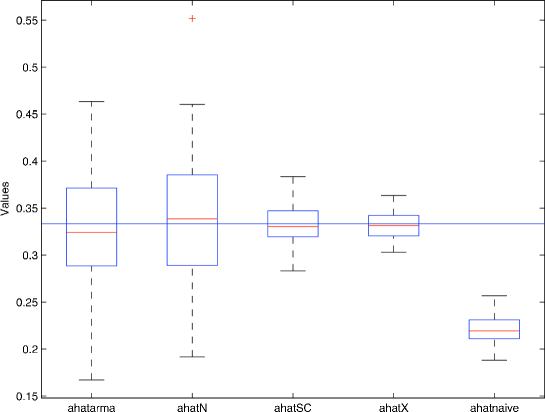
Figure 1. Results for linear Case B and Gaussian error, with $n=5000$ and $\sigma_{\varepsilon}^{2}/\mbox{Var}(X)=0.5$. Box plots of the five estimators $\widehat{a}_{arma}$, $\widehat{a}_{N}$, $\widehat{a}_{SC}$, $\widehat{a}_{X}$ and $\widehat{a}_{naive}$, from left to right, based on 100 replications. True value is $1/3$ (horizontal line).

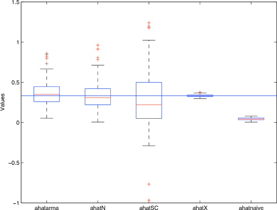
Figure 2. Results for linear Case B and Gaussian error, with $n=5000$ and $\sigma_{\varepsilon}^{2}/\mbox{Var}(X)=6$. Box plots of the five estimators $\widehat{a}_{arma}$, $\widehat{a}_{N}$, $\widehat{a}_{SC}$, $\widehat{a}_{X}$ and $\widehat{a}_{naive}$, from left to right, based on 100 replications. True value is $1/3$ (horizontal line).

The first thing to notice is that, not surprisingly, $\widehat{\theta}_{naive}$ presents a bias, whatever the values of $n$, $s2n$ and the error distribution. The estimator $\widehat{\theta}_{X}$ has the good expected properties (unbiased and small MSE), but it is based on the observation of the $X_{i}$’s. The previously known estimator $\widehat{\theta}_{arma}$ has good asymptotic properties. However its bias is often larger than the biases of $\widehat{\theta}_{N}$ and $\widehat{\theta}_{SC}$, except when $s2n=0.5$ and $\varepsilon$ is Gaussian.

We now consider the two estimators $\widehat{\theta}_{N}$ and $\widehat{\theta}_{SC}$. Recall that their construction requires the choice of $w$. Note first that, whatever the weight function $w$, the two estimators $\widehat{\theta}_{N}$ and $\widehat{\theta}_{SC}$ present good convergence properties. Their biases and MSEs decrease when $n$ increases. When compared one to another, we can see that their numerical behaviors are not the same. Namely for not too large $s2n$, $\widehat{\theta}_{SC}$ has a MSE smaller than $\widehat{\theta}_{N}$ (see Figure 1 and Tables 1-4, when $s2n\leq 3$). With large $s2n$, the estimator $\widehat{\theta}_{N}$ seems to have better properties (see Figure 2 when $s2n=6$). This is expected since $N$ depends on $\sigma_{\varepsilon}^{2}$ and is thus more sensitive to small values of $\sigma_{\varepsilon}^{2}$. The error distribution seems to have a slight infuence on the MSEs of the two estimators. The MSEs are often smaller when $f_{\varepsilon}$ is the Laplace density. This may be related with the theoretical properties in density deconvolution. In that context it is well known that the rate of convergence is slower when $f_{\varepsilon}$ is the Gaussian density. The two estimators $\widehat{\theta}_{N}$ and $\widehat{\theta}_{SC}$ have comparable numerical behaviors in the two linear autoregressive models. Let us recall that in both cases, the simulated chain $X$ are non-mixing but are $\tau$-dependent. In Case A, the stationary distribution of $X$ is continuous whereas it is not the case in Case B. This explains the relative bad properties of $\widehat{\theta}_{arma}$ in Case B. Indeed, due to its construction, this estimator is expected to have good properties when the stationary distribution of the Markov Chain is close to the Gaussian distribution. On the contrary our estimators have similar behavior in both cases.

4.2. Cauchy regression model

We consider the model (1.3) with $f_{\theta}(x)=\theta/(1+x^{2})=\theta f(x)$. The true parameter is $\theta^{0}=1.5$. For the law of $\xi_{0}$ we take $\xi_{0}\sim\mathcal{N}(0,0.01)$. In this case, an empirical study shows that $\sigma_{X}^{2}$ is about 0.1. Moreover $\alpha_{{\bf X}}(k)=O(\kappa^{k})$ for some $\kappa\in]0,1[$ and the Markov chain is $\alpha$-mixing (see Appendix A.2). For $w$ suitably chosen, Theorem 3.2 applies and states that $\hat{\theta}$ is asymptotically normal. For the simulation, we start with $X_{0}$ uniformly distributed over $[0,1]$, and we consider that the chain is close to the stationary chain after 1000 iterations. We then set $X_{i}=X_{i+1000}$.

To our knowledge, the estimator $\widehat{\theta}$ is the first consistent estimator in the literature for this regression function. We first detail the estimator for two choices of the weight function $w$. Then we recall the classic estimator when $X$ is directly observed and the so-called naive estimator.

4.2.1. Expression of the estimator

We consider the two following weight functions:

(4.20) $$N_{c}(x)=(1+x^{2})^{2}\exp\{-x^{2}/(4\sigma_{\varepsilon}^{2})\}\mbox{ and }SC_{c}(x)=(1+x^{2})^{2}\frac{1}{2\pi}\Big{(}\frac{2*\sin(x)}{x}\Big{)}^{4},$$

with $\sigma_{\varepsilon}^{2}$ the variance of $\varepsilon$. This choice of $w$ ensures that Conditions ($\mathbf{C_{1}}$)-($\mathbf{C_{5}}$) hold and our method allows to achieve the parametric rate of convergence. As in the linear case, these two weight functions differ by their dependence on $\sigma_{\varepsilon}^{2}$ and their smoothness properties. The two associated estimators are based on the calculation of $S_{n}(\theta)$, which can be written as

$$S_{n}(\theta)=\frac{1}{n}\sum_{k=1}^{n}[Z_{k}^{2}I_{w}(Z_{k-1})+\theta^{2}I_{wf^{2}}(Z_{k-1})-2\theta Z_{k}I_{wf}(Z_{k-1})],$$

where

$$I_{w}(Z) = \frac{1}{2\pi}\mathbb{R}e\int(w)^{*}(u)\frac{e^{-iuZ}}{f_{\varepsilon}^{*}(-u)}du,\qquad I_{wf}(Z)=\frac{1}{2\pi}\mathbb{R}e\int(wf)^{*}(u)\frac{e^{-iuZ}}{f_{\varepsilon}^{*}(-u)}du$$

$$\mbox{and}\quad I_{wf^{2}}(Z) = \frac{1}{2\pi}\mathbb{R}e\int(wf^{2})^{*}(u)\frac{e^{-iuZ}}{f_{\varepsilon}^{*}(-u)}du.$$

The estimator can be expressed as

(4.21) $$\widehat{\theta}=\frac{\sum_{k=1}^{n}Z_{k}I_{wf}(Z_{k-1})}{\sum_{k=1}^{n}I_{wf^{2}}(Z_{k-1})}.$$

In the following we denote by $I_{wf,N_{c}}(Z)$, $I_{wf^{2},N_{c}}(Z)$, $I_{wf,SC_{c}}(Z)$ and $I_{wf^{2},SC_{c}}(Z)$ respectively, the previous integrals when the weight function is either $w=N_{c}$ or $w=SC_{c}$. In the same way we denote by $\widehat{\theta}_{N_{c}}$ and $\widehat{\theta}_{SC_{c}}$ the corresponding estimators of $\theta^{0}$.

$\bullet$ When $w=N_{c}$, Fourier calculations provide that

$$(N_{c}f)^{*}(t) = \sqrt{2\pi}\sqrt{2\sigma_{\varepsilon}^{2}}\exp(-\sigma_{\varepsilon}^{2}t^{2})\big{(}1+2\sigma_{\varepsilon}^{2}(1-2\sigma_{\varepsilon}^{2}t^{2})\big{)}$$

$$\mbox{ and }(N_{c}f^{2})^{*}(t) = \sqrt{2\pi}\sqrt{2\sigma_{\varepsilon}^{2}}\exp(-\sigma_{\varepsilon}^{2}t^{2}).$$

Now, we can calculate the integrals $I_{wf,N_{c}}(Z)$ and $I_{wf^{2},N_{c}}(Z)$.

If $f_{\varepsilon}$ is the Laplace distribution (4.10), replacing $f_{\varepsilon}^{*}$ by its expression we obtain

$$I_{wf,N_{c}}(Z) = \exp(-Z^{2}/(4\sigma^{2}_{\varepsilon}))\left[Z^{4}-18Z^{2}\sigma_{\varepsilon}^{2}+Z^{2}+8\sigma_{\varepsilon}^{4}-10\sigma_{\varepsilon}^{2}\right]/(8\sigma_{\varepsilon}^{2}),$$

$$\mbox{ and }I_{wf^{2},N_{c}}(Z) = \exp(-Z^{2}/(4\sigma^{2}_{\varepsilon}))\big{[}1+\frac{1}{4}\big{(}1-\frac{Z^{2}}{2\sigma^{2}_{\varepsilon}}\big{)}\big{]}.$$

If $f_{\varepsilon}$ is the Gaussian distribution (4.11), replacing $f_{\varepsilon}^{*}$ by its expression we obtain

$$I_{wf,N_{c}}(Z)=\sqrt{2}e^{-Z^{2}/(2\sigma_{\varepsilon}^{2})}(1-2\sigma_{\varepsilon}^{2}+4Z^{2}),\ \text{and}\quad I_{wf^{2},N_{c}}(Z)=\sqrt{2}e^{-Z^{2}/(2\sigma_{\varepsilon}^{2})}.$$

$\bullet$ When $w=SC_{c}$, easy calculations show that

$$I_{wf,SC_{c}}(Z)=I_{0,SC}(Z)+I_{2,SC}(Z)\mbox{ and }I_{wf^{2},SC_{c}}(Z)=I_{0,SC}(Z),$$

where $I_{0,SC}(Z)$ and $I_{2,SC}(Z)$ are defined by (4.18). As explained before, the integrals $I_{0,SC}(Z)$ and $I_{2,SC}(Z)$ have no explicit form, whatever the error distributions, and are numerically approximated via the IFFT function.

4.2.2. Comparison with classical estimators.

We compare our estimators with two classical estimators, the usual least square estimator without observation noise, and the naive estimator.

$\bullet$ Estimator without noise. When $\varepsilon_{i}=0$, that is $(X_{0},\ldots,X_{n})$ is observed without errors, the parameter can be easily estimated by the usual least square estimator

$$\widehat{\theta}_{X}=\frac{\sum_{i=1}^{n}X_{i}f(X_{i-1})}{\sum_{i=1}^{n}f^{2}(X_{i-1})}.$$

$\bullet$ Naive estimator. The idea for the construction of the naive estimator is to replace the unobserved $X_{i}$ by the observation $Z_{i}$ in the expression of $\widehat{\theta}_{X}$ to get

$$\widehat{\theta}_{naive}=\frac{\sum_{i=1}^{n}Z_{i}f(Z_{i-1})}{\sum_{i=1}^{n}f^{2}(Z_{i-1})}.$$

Classical results show that $\widehat{\theta}_{naive}$ is an asymptotically biased estimator of $\theta^{0}$, which is confirmed by the simulation study.

4.2.3. Simulations results

For each error distribution, we simulate 100 samples with size $n$, $n=500$, $5000$ and $10000$. We consider different values of $\sigma_{\varepsilon}$ such that the ratio signal to noise $s2n=\sigma_{\varepsilon}^{2}/\mbox{Var}(X)$ is $0.5,1.5$ or $3$.

The comparison of the four estimators is based on the bias, the Mean Squared Error (MSE), and the box plots. The results are presented in Figure 3 and Tables 5-6.

The first thing to notice is that, not surprisingly, $\widehat{\theta}_{naive}$ presents a bias, whatever the values of $n$, $s2n$ and the errors distribution. Moreover it converges to (false) values which are different according to $s2n$ (see Tables (5)-(6)).

The estimator $\widehat{\theta}_{X}$ has the good expected properties (unbiased and small MSE), but it is based on the observation of the $X_{i}$’s.

We now compare our two estimators illustrating the influence of $w$, $s2n$ and $f_{\varepsilon}$. Globally, whatever the weight function $w$, the two estimators $\widehat{\theta}$ present good convergence properties. Their biases and MSEs decrease when $n$ increases. The MSEs of $\widehat{\theta}_{SC_{c}}$ increase when $s2n$ increases. This is not the case for the MSE of $\widehat{\theta}_{N_{c}}$. This is probably due to the fact that the weight function chosen for the construction of $\widehat{\theta}_{N_{c}}$ depends on $\sigma_{\varepsilon}^{2}$. This estimator is thus more adaptive to changes in $s2n$.

	ratio		Estimator
n	s2n	$\widehat{\theta}_{N_{c}}(MSE)$	$\widehat{\theta}_{SC_{c}}(MSE)$	$\widehat{\theta}_{X}(MSE)$	$\widehat{\theta}_{naive}(MSE)$
$1000$	0.5	1.5095 (0.0042)	1.5024 (0.0006)	1.5004 (0.0000)	1.4333 (0.0050)
	1.5	1.5006 (0.0021)	1.5005 (0.0013)	1.5002 (0.0000)	1.3657 (0.0190)
	3	1.5017 (0.0024)	1.5005 (0.0024)	1.5002 (0.0000)	1.3267 (0.0314)
$5000$	0.5	1.5045 (0.0008)	1.5005 (0.0001)	1.5003 (0.0000)	1.4320 (0.0047)
	1.5	1.5003 (0.0004)	1.4994 (0.0003)	1.4997 (0.0000)	1.3647 (0.0185)
	3	1.4989 (0.0005)	1.4992 (0.0005)	1.5000 (0.0000)	1.3223 (0.0318)
$10000$	0.5	1.5033 (0.0004)	1.5002 (0.0001)	1.5000 (0.0000)	1.4315 (0.0047)
	1.5	1.5000 (0.0002)	1.5000 (0.0001)	1.4998 (0.0000)	1.3650 (0.0183)
	3	1.4972 (0.0002)	1.4970 (0.0002)	1.4998 (0.0000)	1.3222 (0.0317)

Table 5. Estimation results for Cauchy, Laplace error. Mean estimated values of the four estimators $\widehat{\theta}_{N_{c}}$, $\widehat{\theta}_{SC_{c}}$, $\widehat{\theta}_{X}$ and $\widehat{\theta}_{naive}$ are presented for various values of $n$ ($1000$, 5000 or 10000) and s2n (0.5, 1.5, 3). True value is $\theta^{0}=1.5$. MSE are given in brackets.

	ratio	Estimator
n	s2n	$\widehat{\theta}_{N_{c}}(MSE)$	$\widehat{\theta}_{SC_{c}}(MSE)$	$\widehat{\theta}_{X}(MSE)$	$\widehat{\theta}_{naive}(MSE)$
$1000$	0.5	1.4979 (0.0027)	1.4998 (0.0006)	1.5000 (0.0000)	1.4230 (0.0064)
	1.5	1.4995 (0.0029)	1.5001 (0.0015)	1.5005 (0.0000)	1.3336 (0.0287)
	3	1.5080 (0.0049)	1.5058 (0.0042)	1.4997 (0.0000)	1.2832 (0.0487)
$5000$	0.5	1.5033 (0.0006)	1.5011 (0.0001)	1.4999 (0.0000)	1.4250 (0.0057)
	1.5	1.5011 (0.0004)	1.5001 (0.0003)	1.4999 (0.0000)	1.3351 (0.0274)
	3	1.4998 (0.0009)	1.4996 (0.0008)	1.5002 (0.0000)	1.2767 (0.0501)
$10000$	0.5	1.5017 (0.0003)	1.4997 (0.0000)	1.4996 (0.0000)	1.4236 (0.0059)
	1.5	1.5025 (0.0003)	1.5027 (0.0002)	1.5001 (0.0000)	1.3375 (0.0265)
	3	1.5016 (0.0004)	1.5021 (0.0004)	1.5002 (0.0000)	1.2778 (0.0495)

Table 6. Estimation results for Cauchy, Gaussian error. Mean estimated values of the four estimators $\widehat{\theta}_{N_{c}}$, $\widehat{\theta}_{SC_{c}}$, $\widehat{\theta}_{X}$ and $\widehat{\theta}_{naive}$ are presented for various values of $n$ ($1000$, 5000 or 10000) and s2n (0.5, 1.5, 3). True value is $\theta^{0}=1.5$. MSE are given in brackets.

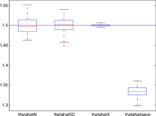
Figure 3. Results for Cauchy and Gaussian error, with $n=5000$ and $\sigma_{\varepsilon}^{2}/\mbox{Var}(X)=1.5$. Box plots of the four estimators $\widehat{\theta}_{N_{c}}$, $\widehat{\theta}_{SC_{c}}$, $\widehat{\theta}_{X}$ and $\widehat{\theta}_{naive}$, from left to right, based on 100 replications. True value is $1.5$ (horizontal line).

5. A more general estimator

For a large number of regression functions, a weight function $w$ such as the one involved in the definition of the estimator $\hat{\theta}$ can be easily exhibited. Nevertheless for some specific regression functions, it seems not straightforward to find a weight function such that $(wf_{\theta})^{*}/f_{\varepsilon}^{*}$ and $(wf_{\theta}^{2})^{*}/f_{\varepsilon}^{*}$ are integrable. We refer to Butucea and Taupin buttaupin for a more complete discussion on this subject. Therefore, we propose a generalization of this estimator to relax these conditions.

5.1. Definition of the general estimator

The key idea for this construction is the following. We introduce a density deconvolution kernel $K_{n,C_{n}}$ defined via its Fourier transform $K_{n,C_{n}}^{*}$ by

(5.22) $$K_{n,C_{n}}^{*}(t)=\frac{K^{*}(t/C_{n})}{f_{\varepsilon}^{*}(-t)}:=\frac{K_{C_{n}}^{*}(t)}{f_{\varepsilon}^{*}(-t)},$$

where $K^{*}$ is the Fourier transform of a kernel $K$ and $C_{n}$ is a sequence which tends to infinity with $n$. The kernel $K$ belongs to ${\mathbb{L}}^{2}({\mathbb{R}})$. Its Fourier transform $K^{*}$ is compactly supported and satisfies $|1-K^{*}(t)|\leq{{{1}}{\mathrm{I}}}_{|t|\geq 1}$. Then, for any integrable function $\Phi$, one has $\lim_{n\to\infty}n^{-1}\sum_{i=1}^{n}\Phi\star K_{n,C_{n}}(Z_{i})=\mathbb{E}(\Phi(X))$. Hence we estimate $\mathbb{E}(\Phi(X))$ by $n^{-1}\sum_{i=1}^{n}\Phi\star K_{n,C_{n}}(Z_{i})$ instead of $n^{-1}\sum_{i=1}^{n}\Phi(X_{i})$ which is not available. We then propose to estimate $S_{\theta^{0},P_{X}}(\theta)$ by

(5.23) $$S_{n}(\theta)=\frac{1}{n}\sum_{i=1}^{n}\mathbb{R}e\left[\big{(}(Z_{i}-f_{\theta})^{2}w\big{)}\star K_{n,C_{n}}(Z_{i-1})\right]\\ =\frac{1}{n}\sum_{i=1}^{n}\mathbb{R}e\!\!\int\!\!\left(Z_{i}-f_{\theta}(x)\right)^{2}w(x)\,K_{n,C_{n}}(Z_{i-1}-x)dx.$$

Using this more general empirical criterion we propose to estimate $\theta^{0}$ by

(5.24) $$\widehat{\theta}=\arg\min_{\theta\in\Theta}S_{n}(\theta).$$

Note that the general construction relies to a truncation of integrals in (2.6). Also note that this general construction still works under Conditions ($\mathbf{C_{1}}$)-($\mathbf{C_{5}}$). It suffices to chose $K^{*}(t/C_{n})={{{1}}{\mathrm{I}}}_{|t|\leq C_{n}}$ with $C_{n}=+\infty$.

5.2. Asymptotic properties under general assumptions

This section presents the asymptotic properties of $\widehat{\theta}$ defined by (5.24) under milder conditions than conditions ($\mathbf{C_{1}}$)-($\mathbf{C_{5}}$), when one cannot exhibit a weight function $w$ ensuring that these conditions hold. In this context the estimator is still consistent, but with a rate which is not necessarily the parametric rate. For the sake of simplicity we only consider the case of $\alpha$-mixing Markov chains.

We assume that

($$\mathbf{A_{3}} \mbox{On }\Theta^{0},\mbox{ the quantity }w^{2}(X_{0})(Z_{1}-f_{\theta}(X_{0}))^{4}\mbox{ and the absolute values of its derivatives}$$)

$$\mbox{ with respect to }\theta\mbox{ up to order 2 }\mbox{ have a finite expectation.}$$

($$\mathbf{A_{4}} \mbox{ The quantity }\sup_{n}\sup_{j\in\{1,\cdots,d\}}\mathbb{E}\Big{(}\sup_{\theta\in\Theta^{\circ}}\Big{|}\frac{\partial}{\partial\theta_{j}}S_{n}(\theta)\Big{|}\Big{)}\mbox{ is finite. }$$)

($$\mathbf{A_{5}} \sup_{\theta\in\Theta}|wf_{\theta}|,\,|w|\mbox{ and }\sup_{\theta\in\Theta}|wf^{2}_{\theta}|\mbox{ belong to }\mathbb{L}_{1}(\mathbb{R}).$$)

We say that a function $\psi\in\mathbb{L}_{1}(\mathbb{R})$ satisfies (5.25) if for a sequence $C_{n}$ we have

(5.25) $$\min_{q=1,2}\parallel\psi^{*}(K_{C_{n}}^{*}-1)\parallel_{q}^{2}+n^{-1}\min_{q=1,2}\left\|\frac{\psi^{*}K_{C_{n}}^{*}}{f_{\varepsilon}^{*}}\right\|_{q}^{2}=o(1).$$

Theorem 5.1.

Under the assumptions ($\mathbf{I1_{1}}$), ($\mathbf{I1_{2}}$), ($\mathbf{N_{1}}$), ($\mathbf{A_{1}}$) ($\mathbf{A_{3}}$) - ($\mathbf{A_{5}}$), let $\widehat{\theta}$ be defined by (5.24) with $C_{n}$ such that (5.25) holds for $w$, $wf_{\theta}$ and $wf_{\theta}^{2}$ and their first derivatives with respect to $\theta$. Assume that the sequence $(X_{k})$ is $\alpha$-mixing that is

$$\alpha_{\bf X}(k)\mathrel{\mathop{\kern 0.0pt\ \longrightarrow\ }\limits_{n\to\infty}}0,\mbox{ as }k\mathrel{\mathop{\kern 0.0pt\ \longrightarrow\ }\limits_{n\to\infty}}\infty.$$

Then $\mathbb{E}(\|\widehat{\theta}-\theta^{0}\|_{\ell^{2}}^{2})=o(1),$ as $n\to\infty$ and $\widehat{\theta}$ is a consistent estimator of $\theta^{0}.$

We now give upper bounds for the rates of convergence under two different types of assumptions:

($$\mathbf{A_{6}} X_{0}\mbox{ admits a density }f_{X}\mbox{ with respect to the Lebesgue measure and there exist two }$$)

$$\mbox{ constants }C_{1}(f_{\theta^{0}}^{2})\mbox{ and }C_{2}(f_{\theta^{0}})\mbox{ such that }\parallel f_{\theta^{0}}f_{X}\parallel_{2}^{2}\leq C_{1}(f_{\theta^{0}}),\mbox{ and }$$

$$\parallel f_{\theta^{0}}^{2}f_{X}\parallel_{2}^{2}\leq C_{2}(f_{\theta^{0}}^{2}).$$

($$\mathbf{A_{7}} \sup_{z\in\mathbb{R}}\mathbb{E}[f_{\theta^{0}}^{2}(X_{0})f_{\varepsilon}(z-X_{0})]\mbox{ and }\sup_{z\in\mathbb{R}}\mathbb{E}[f_{\varepsilon}(z-X_{0})]\mbox{ are finite.}$$)

These two assumptions are mostly required for technical reasons. The following theorem still holds when $X_{0}$ does not admit a density, under a slightly different moment assumption.

Theorem 5.2.

Suppose that the assumptions of Theorem 5.1 hold. Assume moreover that the sequence $(X_{k})_{k\geq 0}$ is $\alpha$-mixing with $\sum_{k\geq 1}\sqrt{\alpha_{\bf X}(k)}<\infty$, and that, for all $\theta\in\Theta$, the functions $w$, $f_{\theta}w$ and $f_{\theta}^{2}w$ and their derivatives up to order 3 with respect to $\theta$ satisfy (5.25).

1) Assume that the sequence $X_{0}$ admits a density with respect to the Lebesgue measure and that Assumption ($\mathbf{A_{6}}$) holds. Then $\widehat{\theta}-\theta^{0}=O_{p}(\varphi_{n}^{2})$ with $\varphi_{n}=\|(\varphi_{n,j})\|_{\ell^{2}}$, $\varphi_{n,j}^{2}=B_{n,j}^{2}+V_{n,j}/n$, $j=1\ldots,d$, where

$$B_{n,j}\!\! = \!\!\min\left\{B_{n,j}^{[1]},B_{n,j}^{[2]}\right\}\mbox{ and }V_{n,j}\!\!=\!\!\min\left\{V_{n,j}^{[1]},V_{n,j}^{[2]}\right\}$$

and for $q=1,2$

$$B_{n,j}^{[q]} = \left\|(wf^{(1)}_{\theta,j})^{*}(K_{C_{n}}^{*}-1)\right\|^{2}_{q}+\left\|(wf_{\theta^{0}}f^{(1)}_{\theta^{0},j})^{*}(K_{C_{n}}^{*}-1)\right\|^{2}_{q},$$

and

$$V_{n,j}^{[q]}\!\! = \left\|(wf^{(1)}_{\theta^{0},j})^{*}\frac{K_{C_{n}}^{*}}{f_{\varepsilon}^{*}}\right\|_{q}^{2}+\left\|(wf_{\theta^{0}}f^{(1)}_{\theta^{0},j})^{*}\frac{K_{C_{n}}^{*}}{f_{\varepsilon}^{*}}\right\|_{q}^{2}.$$

2) Assume that ($\mathbf{A_{7}}$) holds. Then $\widehat{\theta}-\theta^{0}=O_{p}(\varphi_{n}^{2})$ with $\varphi_{n}=\|(\varphi_{n,j})\|_{\ell^{2}}$, $\varphi_{n,j}^{2}=B_{n,j}^{2}+V_{n,j}/n$, $j=1\ldots,d$, where $B_{n,j}=B_{n,j}^{[1]}\mbox{ and }V_{n,j}=\min\left\{V_{n,j}^{[1]},V_{n,j}^{[2]}\right\}.$

This theorem states an upper bound for the quadratic risk under very general conditions. It holds under mild conditions on $w$, $f_{\theta}$ and $f_{\varepsilon}$. We refer to Table 1 in Butucea and Taupin buttaupin for more details on the resulting rates.

Appendix A Properties of the dependence coefficients and examples

A.1. Covariance inequalities and coupling

The following results are the key arguments to prove the asymptotic normality of $\widehat{\theta}$. We keep the same notations as in Definition 3.1.

We first recall a covariance inequality due to Rio Rio93. For any positive random variable $Z$, let $Q_{Z}$ be the inverse cadlag of the tail function $t\to{\mathbb{P}}(Z>t)$. Let $X$ and $Y$ be two real valued random variables such that $\text{Cov}(X,Y)$ is well defined. The following inequality holds

(A.26) $$|\text{Cov}(Y,X)|\leq 4\int_{0}^{\alpha(\sigma(Y),\sigma(X))}Q_{|X|}(u)Q_{|Y|}(u)du\,.$$

Next, we recall the coupling properties of $\tau$ (see Dedecker and Prieur JDCPCoeff): enlarging $\Omega$ if necessary, there exists $X^{*}$ distributed as $X$ and independent of ${\mathcal{M}}$ such that

(A.27) $$\tau({\mathcal{M}},X)={\mathbb{E}}(\|X-X^{*}\|_{\mathbb{B}})\,.$$

A.2. Dependence properties of autoregressive models

We recall here the mixing properties of the autoregressive models

$$X_{i}=f_{\theta^{0}}(X_{i-1})+\xi_{i},$$

that have been described in particular in the papers by Mokkadem Mokkadem85 and Ango-Nzé AngoNze. For instance, assume that

• the law of $\xi_{0}$ has a density $f_{\xi}$ such that $f_{\xi}>c>0$ on a neighborhood of zero, and there exists $S\geq 1$ such that ${\mathbb{E}}(|\xi_{0}|^{S})<\infty$.

• $f_{\theta^{0}}$ is continuous and there exist $R\geq 1$ and $\rho\in]0,1[$ such that: for any $|x|\geq R$, $|f_{\theta^{0}}(x)|\leq\rho|x|$.

Then there exists a unique invariant probability measure, and the stationary Markov chain $(X_{i})_{i\geq 0}$ satisfies $\alpha_{{\bf X}}(k)=O(\kappa^{k})$ for any $\kappa\in]\rho,1[$ and is $\alpha$-mixing.

Now if the second point is weakened to

• $f_{\theta^{0}}$ is continuous and there exist $R\geq 1$ and $\delta\in]0,1[$ such that: for any $|x|\geq R$, $|f_{\theta^{0}}(x)|\leq|x|(1-|x|^{-\delta})$.

Then there exists a unique invariant probability measure, and the stationary Markov chain $(X_{i})_{i\geq 0}$ satisfies $\alpha_{{\bf X}}(k)=O(k^{1-S/\delta})$ and is $\alpha$-mixing.

Now, if we do not assume that $\xi_{0}$ has a density, then the chain may not be $\alpha$-mixing (and not even irreducible). However, under appropriate assumptions on $f_{\theta^{0}}$, it is still possible to obtain upper bounds for the coefficient $\tau$. For instance assume that

• there exists $S\geq 1$ such that ${\mathbb{E}}(|\xi_{0}|^{S})<\infty$.

• $|f_{\theta^{0}}(x)-f_{\theta^{0}}(y)|\leq\rho|x-y|$ for some $\rho\in]0,1[$.

Then there exists a unique invariant probability measure, and the stationary Markov chain $(X_{i})_{i\geq 0}$ satisfies $\tau_{{\bf X},2}(k)=O(\rho^{k})$ and is $\tau$-dependent. Now if the second point is weakened to

• there exist $\delta$ in $[0,1[$ and $C$ in $]0,1]$ such that $|f^{\prime}(t)|\leq 1-C(1+|t|)^{-\delta}$ almost everywhere.

Then there exists a unique invariant probability measure, and for $S>1+\delta$ the stationary Markov chain $(X_{i})_{i\geq 0}$ satisfies $\tau_{{\bf X},2}(n)=O(n^{(\delta+1-S)/\delta})$ and is $\tau$-dependent.

Appendix B proofs of Theorems

B.1. Proof of Theorem 3.1

The main point of the proof consists in showing the two following points

i) for any $\theta$ in $\Theta$, $S_{n}(\theta)\mathrel{\mathop{\kern 0.0pt\ \longrightarrow\ }\limits_{n\to\infty}^{{\mathbb{L}^{1}}}}S_{\theta^{0},P_{X}}(\theta)$, with $S_{\theta^{0},P_{X}}(\theta)$ admitting a unique minimum in $\theta=\theta^{0}$.

ii) For $\omega_{2}(n,\rho)$ defined as $\omega_{2}(n,\rho)=\sup\left\{|S_{n}(\theta)-S_{n}(\theta^{\prime})|:\|\theta-\theta^{\prime}\|_{\ell^{2}}\leq\rho\right\},$ there exists a sequence $\rho_{k}$ tending to 0, such that

(B.1) $${\mathbb{E}}(\omega_{2}(n,\rho_{k}))=O(\rho_{k}).$$

Let us start with the proof of i) by writing that

$$S_{n}(\theta)=\frac{1}{n}\sum_{k=1}^{n}\Psi(Z_{k},Z_{k-1}),\mbox{ with }\Psi(Z_{1},Z_{0})=\frac{1}{2\pi}\mathbb{R}e\int\frac{\left(\big{(}Z_{1}-f_{\theta}\big{)}^{2}w\right)^{*}(t)e^{-itZ_{0}}}{f_{\varepsilon}^{*}(-t)}dt,$$

that is seen as a function of a strictly stationary and ergodic sequence of random variables. By the ergodic theorem and Assumption ($\mathbf{A_{2}}$) we conclude that for any $\theta\in\Theta$,

$$S_{n}(\theta)\mathrel{\mathop{\kern 0.0pt\ \longrightarrow\ }\limits_{n\to\infty}^{{\mathbb{L}^{1}}}}\mathbb{E}(\psi(Z_{1},Z_{0}))=S_{\theta^{0},P_{X}}(\theta).$$

It remains now to check that there exists a sequence $\rho_{k}$ tending to 0, such that (B.1) holds. This follows by the assumption ($\mathbf{C_{2}}$) and by writing that

(B.2) $$\sup_{\parallel\theta-\theta^{\prime}\parallel_{\ell^{2}}\leq\rho}|S_{n}(\theta)-S_{n}(\theta^{\prime})|\leq\sup_{\parallel\theta-\theta^{\prime}\parallel_{\ell^{2}}\leq\rho}\parallel\theta-\theta^{\prime}\parallel_{\ell^{2}}\sup_{\theta\in\Theta^{0}}\parallel S^{(1)}_{n}(\theta)\parallel_{\ell^{2}}.$$

∎

B.2. Proof of Theorem 3.2

By using a Taylor expansion based on the smoothness properties of $\theta\mapsto wf_{\theta}$ and the consistency of $\widehat{\theta}$, we obtain

$$0=S^{(1)}_{n}(\widehat{\theta})=S^{(1)}_{n}(\theta^{0})+S^{(2)}_{n}(\theta^{0})(\widehat{\theta}-\theta^{0})+R_{n}(\widehat{\theta}-\theta^{0}),$$

with $R_{n}$ defined by

(B.3) $$R_{n}=\int_{0}^{1}[S^{(2)}_{n}(\theta^{0}+s(\widehat{\theta}-\theta^{0}))-S^{(2)}_{n}(\theta^{0})]ds.$$

This implies that

(B.4) $$\widehat{\theta}-\theta^{0}=-[S^{(2)}_{n}(\theta^{0})+R_{n}]^{-1}S^{(1)}_{n}(\theta^{0}).$$

Consequently, we have to check the three following points.

• $\sqrt{n}S^{(1)}_{n}(\theta^{0})\mathrel{\mathop{\kern 0.0pt\ \longrightarrow\ }\limits_{n\to\infty}^{{\mathcal{L}}}}\mathcal{N}(0,\Sigma_{0,1})$;

• $S^{(2)}_{n}(\theta^{0})\mathrel{\mathop{\kern 0.0pt\ \longrightarrow\ }\limits_{n\to\infty}^{{\mathrm{I}\!\mathrm{P}}}}S^{(2)}_{\theta^{0},P_{X}}(\theta^{0});$

• $R_{n}$ defined in (B.3) satisfies $R_{n}\mathrel{\mathop{\kern 0.0pt\ \longrightarrow\ }\limits_{n\to\infty}^{{\mathrm{I}\!\mathrm{P}}}}0.$

Note that the covariance matrix $\Sigma_{0,1}$ in i) satisfies $\Sigma_{0,1}=\Sigma/4\pi^{2}$, with $\Sigma$ defined by the equation (B.6) below. Consequently, according to ii) and iii), the covariance matrix $\Sigma_{1}$ satisfies

(B.5) $$\Sigma_{1}=\frac{1}{4\pi^{2}}(S^{(2)}_{\theta^{0},P_{X}}(\theta^{0}))^{-1}\Sigma(S^{(2)}_{\theta^{0},P_{X}}(\theta^{0}))^{-1},\quad\text{with $\Sigma$ defined by (\ref{somcov})}.$$

Proof of i)

Under Assumption ($\mathbf{C_{2}}$),

$$\left(\sqrt{n}S^{(1)}_{n}(\theta^{0})\right)_{i}=\frac{1}{2\pi\sqrt{n}}\sum_{k=1}^{n}\mathbb{R}e\int\left(\frac{\partial}{\partial\theta_{i}}((Z_{k}-f_{\theta})^{2})w\Big{|}_{\theta=\theta^{0}}\right)^{*}(t)\frac{e^{-itZ{k-1}}}{f_{\varepsilon}^{*}(-t)}dt.$$

We have thus to prove that

$$\frac{1}{2\pi\sqrt{n}}\sum_{k=1}^{n}\mathbb{R}e\int\big{(}-2(Z_{k}-f_{\theta^{0}})f^{(1)}_{\theta^{0}}w\big{)}^{*}(t)\frac{e^{-itZ{k-1}}}{f_{\varepsilon}^{*}(-t)}dt\mathrel{\mathop{\kern 0.0pt\ \longrightarrow\ }\limits_{n\to\infty}^{{\mathcal{L}}}}\mathcal{N}(0,\Sigma_{0,1}).$$

We first use that $\mathbb{E}(S_{n}(\theta))=S_{\theta^{0},P_{X}}(\theta)$ and thus $\mathbb{E}(S^{(1)}_{n}(\theta^{0}))=S^{(1)}_{\theta^{0},P_{X}}(\theta^{0})=0.$ Next we write

$$\sqrt{n}S^{(1)}_{n}(\theta^{0})=\sqrt{n}S^{(1)}_{n}(\theta^{0})-\mathbb{E}[\sqrt{n}S^{(1)}_{n}(\theta^{0})]=\frac{1}{2\pi\sqrt{n}}\sum_{k=1}^{n}T_{k}$$

with $T_{k}=-2W_{k,1}+2W_{k,2}$, and

$$W_{k,1} = Z_{k}\mathbb{R}e\int\big{(}f^{(1)}_{\theta^{0}}w\big{)}^{*}(t)\frac{e^{-itZ_{k-1}}}{f_{\varepsilon}^{*}(-t)}dt-\mathbb{E}\left[Z_{k}\mathbb{R}e\int\big{(}f^{(1)}_{\theta^{0}}w\big{)}^{*}(t)\frac{e^{-itZ_{k-1}}}{f_{\varepsilon}^{*}(-t)}dt\right]$$

$$W_{k,2} = \mathbb{R}e\int\big{(}f_{\theta^{0}}f^{(1)}_{\theta^{0}}w\big{)}^{*}(t)\frac{e^{-itZ_{k-1}}}{f_{\varepsilon}^{*}(-t)}dt-\mathbb{E}\left[\mathbb{R}e\int\big{(}f_{\theta^{0}}f^{(1)}_{\theta^{0}}w\big{)}^{*}(t)\frac{e^{-itZ_{k-1}}}{f_{\varepsilon}^{*}(-t)}dt\right].$$

Let ${\mathcal{M}}_{1}=\sigma(X_{0},X_{1},\varepsilon_{0},\varepsilon_{1})$. According to Dedecker and Rio DedeckerRio, $n^{-1/2}\sum_{k=1}^{n}T_{k}$ converges to a centered Gaussian vector with covariance matrix

(B.6) $$\Sigma=\mathrm{Cov}(T_{1},T_{1})+2\sum_{k>1}\mathrm{Cov}(T_{1},T_{k})\,,$$

as soon as for any $(p,q)$ in $\{1,\cdots,d\}\times\{1,\cdots,d\}$

(B.7) $$\sum_{k=3}^{\infty}\mathbb{E}|(T_{1})_{p}\mathbb{E}((T_{k})_{q}|\mathcal{M}_{1})|<\infty.$$

For any $(p,q)$ in $\{1,\cdots,d\}\times\{1,\cdots,d\}$ and any $i,j\in\{1,2\}$, we shall give an upper bound for

$$\mathbb{E}\left|(W_{1,i})_{p}\mathbb{E}((W_{k,j})_{q}|\mathcal{M}_{1})\right|.$$

We first notice that the sequence $(\varepsilon_{k},\varepsilon_{k-1})$ is independent of $\mathcal{M}_{1}\vee\sigma(X_{k},X_{k-1})$. It follows that for $i,j\in\{1,2\}$,

$$\mathbb{E}\left|(W_{1,i})_{p}\mathbb{E}((W_{k,j})_{q}|\mathcal{M}_{1})\right|=\mathbb{E}\left|(W_{1,i})_{p}\mathbb{E}((\tilde{W}_{k,j})_{q}|\mathcal{M}_{1})\right|,$$

with

$$(\tilde{W}_{k,1})_{q} = X_{k}\int\big{(}f^{(1)}_{\theta^{0},q}w\big{)}^{*}(t)e^{-itX_{k-1}}dt-\mathbb{E}\left[X_{k}\int\big{(}f^{(1)}_{\theta^{0},q}w\big{)}^{*}(t)e^{-itX_{k-1}}dt\right]$$

$$(\tilde{W}_{k,2})_{q} = \int\big{(}f_{\theta^{0}}f^{(1)}_{\theta^{0},q}w\big{)}^{*}(t)e^{-itX_{k-1}}dt-\mathbb{E}\left[\int\big{(}f_{\theta^{0}}f^{(1)}_{\theta^{0},q}w\big{)}^{*}(t)e^{-itX_{k-1}}dt\right].$$

Next, since ${\mathbb{P}}_{(X_{k-1},X_{k})|\sigma(\varepsilon_{0},\varepsilon_{1},X_{0},X_{1})}={\mathbb{P}}_{(X_{k-1},X_{k})|\sigma(X_{1})}$, we infer that

$$\mathbb{E}\left|(W_{1,i})_{p}\mathbb{E}((W_{k,j})_{q}|\mathcal{M}_{1})\right|=\mathbb{E}\left|(W_{1,i})_{p}\mathbb{E}((\tilde{W}_{k,j})_{q}|X_{1})\right|.$$

Next we use that under Condition ($\mathbf{C_{2}}$),

$$|(W_{1,1})_{p}| \leq |Z_{1}|\int\left|\big{(}f^{(1)}_{\theta^{0},p}w\big{)}^{*}(t)\frac{e^{-itZ_{0}}}{f_{\varepsilon}^{*}(-t)}\right|dt+\mathbb{E}\left\{|Z_{1}|\int\left|\big{(}f^{(1)}_{\theta^{0},p}w\big{)}^{*}(t)\frac{e^{-itZ_{0}}}{f_{\varepsilon}^{*}(-t)}\right|dt\right\}$$

$$\leq |Z_{1}|\int\left|\big{(}f^{(1)}_{\theta^{0},p}w\big{)}^{*}(t)\frac{1}{f_{\varepsilon}^{*}(-t)}\right|dt+\mathbb{E}\left\{|Z_{1}|\int\left|\big{(}f^{(1)}_{\theta^{0},p}w\big{)}^{*}(t)\frac{1}{f_{\varepsilon}^{*}(-t)}\right|dt\right\}$$

$$\leq C_{1}(|Z_{1}|+\mathbb{E}(|Z_{1}|)).$$

In the same way we get that $|(W_{1,2})_{p}|\leq C_{2}$.

Now, since $\varepsilon_{1}$ is independent of $X_{1}$, for $j\in\{1,2\}$

(B.8) $$\mathbb{E}\left|(W_{1,1})_{p}\mathbb{E}((\tilde{W}_{k,j})_{q}|X_{1})\right| \leq C_{1}\mathbb{E}\left[(|Z_{1}|+{\mathbb{E}}(|Z_{1}|))\left|\mathbb{E}((\tilde{W}_{k,j})_{q}|X_{1})\right|\right]$$

$$\leq C\mathbb{E}\left[(|X_{1}|+{\mathbb{E}}(|X_{1}|))\left|\mathbb{E}((\tilde{W}_{k,j})_{q}|X_{1})\right|\right].$$

In the same way

(B.9) $$\mathbb{E}\left|(W_{1,2})_{p}\mathbb{E}((\tilde{W}_{k,j})_{q}|X_{1})\right|\leq C\mathbb{E}\left|\mathbb{E}((\tilde{W}_{k,j})_{q}|X_{1})\right|.$$

Note that

$$\mathbb{E}\left[(|X_{1}|+{\mathbb{E}}(|X_{1}|))\left|\mathbb{E}((\tilde{W}_{k,1})_{q}|X_{1})\right|\right]=\mathrm{Cov}((|X_{1}|+{\mathbb{E}}(|X_{1}|))\text{sign}(\mathbb{E}((\tilde{W}_{k,1})_{q}|X_{1})),(\tilde{W}_{k,1})_{q}).$$

Now, we use the covariance inequality (A.26). Note first that

$$(|X_{1}|+{\mathbb{E}}(|X_{1}|))\text{sign}(\mathbb{E}((\tilde{W}_{k,1})_{q}|X_{1}))\leq|X_{1}|+{\mathbb{E}}(|X_{1}|)$$

and

$$|(\tilde{W}_{1,1})_{q}|\leq D(|X_{1}|+{\mathbb{E}}(|X_{1}|))\,.$$

Since $(X_{i})_{i\geq 0}$ is a strictly stationary Markov chain, it is well known that

(B.10) $$\alpha(\sigma(X_{1}),\sigma(X_{k-1},X_{k}))=\alpha(\sigma(X_{1}),\sigma(X_{k-1}))=\alpha_{\bf X}(k-2)\,.$$

Hence, applying (A.26),

$$\mathbb{E}\left|(W_{1,1})_{p}\mathbb{E}((\tilde{W}_{k,1})_{q}|X_{1})\right|\leq C\int_{0}^{\alpha_{\bf X}(k-2)}Q^{2}_{|X_{1}|}(u)du\,.$$

We conclude that

$$\sum_{k\geq 3}\mathbb{E}\left|(W_{1,1})_{p}\mathbb{E}((W_{k,1})_{q}|\mathcal{M}_{1})\right|\leq C\sum_{k\geq 3}\int_{0}^{\alpha_{\bf X}(k-2)}Q^{2}_{|X_{1}|}(u)du.$$

Finally, using similar arguments for the three quantities $\sum_{k\geq 3}\mathbb{E}\left|(W_{1,2})_{p}\mathbb{E}((W_{k,1})_{q}|\mathcal{M}_{1})\right|$,
$\sum_{k\geq 3}\mathbb{E}\left|(W_{1,1})_{p}\mathbb{E}((W_{k,2})_{q}|\mathcal{M}_{1})\right|$ and $\sum_{k\geq 3}\mathbb{E}\left|(W_{1,2})_{p}\mathbb{E}((W_{k,2})_{q}|\mathcal{M}_{1})\right|$ we conclude that

$$\sqrt{n}S^{(1)}_{n}(\theta^{0})\mathrel{\mathop{\kern 0.0pt\ \longrightarrow\ }\limits_{n\to\infty}^{{\mathcal{L}}}}\mathcal{N}(0,\Sigma/(4\pi^{2}))$$

as soon as

$$\sum_{k\geq 1}\int_{0}^{\alpha_{\bf X}(k)}Q^{2}_{|X_{1}|}(u)du<\infty.$$

∎

Proof of ii)

Under Condition ($\mathbf{C_{3}}$), for $j,k=1,\cdots,d$,

(B.11) $$\left(S^{(2)}_{n}(\theta)\right)_{j,k}=\frac{1}{2\pi n}\sum_{\ell=1}^{n}\mathbb{R}e\int\left(-2Z_{\ell}\frac{\partial^{2}}{\partial\theta_{j}\partial\theta_{k}}(f_{\theta}w)+\frac{\partial^{2}}{\partial\theta_{j}\partial\theta_{k}}(f_{\theta}^{2}w)\right)^{*}(t)\frac{e^{-itZ_{\ell-1}}}{f_{\varepsilon}^{*}(-t)}dt$$

and by applying the ergodic theorem we get that

$$S^{(2)}_{n}(\theta^{0})\mathrel{\mathop{\kern 0.0pt\ \longrightarrow\ }\limits_{n\to\infty}^{{\mathrm{I}\!\mathrm{P}}}}S^{(2)}_{\theta^{0},P_{X}}(\theta^{0}).$$

∎

Proof of iii)

Starting from (B.3) and (B.11), the point iii) follows from the assumption ($\mathbf{C_{4}}$) on the properties of the derivatives at order 3 of $wf_{\theta}$ and $wf_{\theta}^{2}$. ∎

B.3. Proof of Theorem 3.3

We follow the proof of Theorem 3.2 and keep the same notations. We have to check that the condition (B.7) holds. We start from the inequalities (B.8) and (B.9). For clarity, let us write

$$(\tilde{W}_{k,1})_{q}=(\tilde{W}_{k,1})_{q}(X_{k},X_{k-1})\,.$$

Let $\psi_{M}$ be the truncating function defined by $\psi_{M}(x)=(x\wedge M)\vee(-M)$. Applying (A.27), let $(X_{k}^{*},X_{k-1}^{*})$ be the random variable distributed as $(X_{k},X_{k-1})$ and independent of $X_{1}$ such that

$$\frac{1}{2}(\|X_{k}-X_{k}^{*}\|_{1}+\|X_{k-1}-X^{*}_{k-1}\|_{1})=\tau(\sigma(X_{1}),(X_{k-1},X_{k}))\leq\tau_{X,2}(k-2)\,.$$

Define the constants $K_{1}$ and $K_{2}$ by

$$K_{1}=\int\left|\big{(}f^{(1)}_{\theta^{0},q}w\big{)}^{*}(t)\right|dt<\infty\,,\quad K_{2}=\int|t|\left|\big{(}f^{(1)}_{\theta^{0},q}w\big{)}^{*}(t)\right|dt<\infty\,.$$

Clearly

$$|X_{1}\mathbb{E}((\tilde{W}_{k,1})_{q}(X_{k},X_{k-1})|X_{1})|\leq M|\mathbb{E}((\tilde{W}_{k,1})_{q}(X_{k},X_{k-1})|X_{1})|+K_{2}|X_{1}|{\mathbf{1}}_{|X_{1}|>M}(|X_{k}|+{\mathbb{E}}(|X_{k}|))\,.$$

Now, since $(X_{k}^{*},X_{k-1}^{*})$ is independent of $X_{1}$, one has that

$$|\mathbb{E}((\tilde{W}_{k,1})_{q}(X_{k},X_{k-1})|X_{1})|=|\mathbb{E}((\tilde{W}_{k,1})_{q}(X_{k},X_{k-1})-(\tilde{W}_{k,1})_{q}(X^{*}_{k},X^{*}_{k-1})|X_{1})|\,.$$

By definition of $(\tilde{W}_{k,1})_{q}(X_{k},X_{k-1})$, there exists a constant $C$ such that

$$|(\tilde{W}_{k,1})_{q}(X_{k},X_{k-1})-(\tilde{W}_{k,1})_{q}(X^{*}_{k},X^{*}_{k-1})-((\tilde{W}_{k,1})_{q}(\psi_{M}(X_{k}),X_{k-1})-(\tilde{W}_{k,1})_{q}(\psi_{M}(X^{*}_{k}),X^{*}_{k-1}))|\\ \leq C(|X_{k}|{\mathbf{1}}_{|X_{k}|>M}+|X_{k}^{*}|{\mathbf{1}}_{|X_{k}^{*}|>M}).$$

Hence

$$|\mathbb{E}((\tilde{W}_{k,1})_{q}(X_{k},X_{k-1})|X_{1})| \leq |\mathbb{E}((\tilde{W}_{k,1})_{q}(\psi_{M}(X_{k}),X_{k-1})-(\tilde{W}_{k,1})_{q}(\psi_{M}(X^{*}_{k}),X^{*}_{k-1})|X_{1})|$$

$$+ C(|X_{k}|{\mathbf{1}}_{|X_{k}|>M}+|X_{k}^{*}|{\mathbf{1}}_{|X_{k}^{*}|>M})\,.$$

Since $\psi_{M}$ is 1-Lipschitz and bounded by $M$, and since $x\rightarrow\exp(itx)$ is $|t|$-Lipschitz and bounded by 1, under Condition ($\mathbf{C_{5}}$), one has

$$|(\tilde{W}_{k,1})_{q}(\psi_{M}(X_{k}),X_{k-1})-(\tilde{W}_{k,1})_{q}(\psi_{M}(X^{*}_{k}),X^{*}_{k-1})|\leq MK_{2}|X_{k-1}-X_{k-1}^{*}|+K_{1}|X_{k}-X_{k}^{*}|\,.$$

It follows that

$$|X_{1}\mathbb{E}((\tilde{W}_{k,1})_{q}(X_{k},X_{k-1})|X_{1})| \leq K_{2}|X_{1}|{\mathbf{1}}_{|X_{1}|>M}(|X_{k}|+{\mathbb{E}}(|X_{k}|))$$

$$+ M^{2}K_{2}|X_{k-1}-X_{k-1}^{*}|+MK_{1}|X_{k}-X_{k}^{*}|)$$

$$+ CM(|X_{k}|{\mathbf{1}}_{|X_{k}|>M}+|X_{k}^{*}|{\mathbf{1}}_{|X_{k}^{*}|>M})\,.$$

Using that

$$|X_{1}|{\mathbf{1}}_{|X_{1}|>M}|X_{k}|\leq\frac{3}{2}X_{1}^{2}{\mathbf{1}}_{|X_{1}|>M}+\frac{1}{2}X_{k}^{2}{\mathbf{1}}_{|X_{k}|>M}\,,$$

we infer from (B.8) with $j=1$ that there exists a positive constant $K$ such that

$$\mathbb{E}\left[\left|(W_{1,1})_{p}\mathbb{E}((\tilde{W}_{k,1})_{q}|X_{1})\right|\right]\leq K(L(M^{2})+M(M+1)\tau_{{\bf X},2}(k-2))\,,$$

where $L(t)={\mathbb{E}}(X_{0}^{2}{\mathbf{1}}_{X_{0}^{2}>t})$. Let then $G(t)=t^{-1}L(t)$, and let $G^{-1}$ be the inverse cadlag of $G$. Choose then $M^{2}=G^{-1}(\tau_{{\bf X},2}(k-2))$. We obtain that

$$\mathbb{E}\left[\left|(W_{1,1})_{p}\mathbb{E}((\tilde{W}_{k,1})_{q}|X_{1})\right|\right]\leq 2K(2G^{-1}(\tau_{{\bf X},2}(k-2))\tau_{{\bf X},2}(k-2)+\sqrt{G^{-1}(\tau_{{\bf X},2}(k-2))}\tau_{{\bf X},2}(k-2))\,.$$

It follows that

$$\sum_{k\geq 3}\mathbb{E}\left[\left|(W_{1,1})_{p}\mathbb{E}((\tilde{W}_{k,1})_{q}|X_{1})\right|\right]<\infty\quad\text{as soon as}\quad\sum_{k>0}G^{-1}(\tau_{{\bf X},2}(k))\tau_{{\bf X},2}(k)<\infty\,.$$

Easier control holds for the other terms in (B.8) and (B.9). Consequently (B.7) holds as soon as (3.9) holds, and the proof is complete.

B.4. Proof of Theorem 5.1

The proof of the consistency under the assumptions of Theorem 5.1 is quite different from the proof of the consistency under Conditions ($\mathbf{C_{1}}$)-($\mathbf{C_{2}}$) in Theorem 3.1. This comes from the fact that $S_{n}(\theta)$ is now a triangular array of the form

$$S_{n}(\theta)=\frac{1}{n}\sum_{k=1}^{n}\Psi_{n}(Z_{k},Z_{k-1})\mbox{ with }\Psi_{n}(Z_{1},Z_{0})=\frac{1}{2\pi}\mathbb{R}e\int\frac{\left(\big{(}Z_{1}-f_{\theta}\big{)}^{2}w\right)^{*}(t)e^{-itZ_{0}}K_{C_{n}}^{*}(t)}{f_{\varepsilon}^{*}(-t)}dt.$$

In this context we show that

i) For all $\theta$ in $\Theta$, $\mathbb{E}[(S_{n}(\theta)-S_{\theta^{0},P_{X}}(\theta))^{2}]=o(1)$ as $n\to\infty.$

ii) The control (B.1) holds.

Note first that ii) follows from the upper bound (B.2) and Assumption ($\mathbf{A_{4}}$).

For the proof of i) we check that for all $\theta\in\Theta,$

(B.12) $$\mathbb{E}[S_{n}(\theta)]-S_{\theta^{0},P_{X}}(\theta)=o(1)\quad\mbox{ and }\mbox{Var}(S_{n}(\theta))=o(1),\quad\text{ as }n\to\infty.$$

Proof of the first part of $(\ref{cons})$.

Since $Z_{0}=X_{0}+\varepsilon_{0}$, with $\varepsilon_{0}$ independent of $(Z_{1},X_{0})$, it follows that

$$\mathbb{E}[S_{n}(\theta)]=\mathbb{E}\left[\mathbb{R}e\left((Z_{1}-f_{\theta})^{2}\,w\right)\star K_{n,C_{n}}(Z_{0})\right]=\mathbb{E}\left[\left((Z_{1}-f_{\theta})^{2}\,w\right)\star K_{C_{n}}(X_{0})\right]\,,$$

hence

$$\mathbb{E}[S_{n}(\theta)]-S_{\theta^{0},P_{X}}(\theta) = \frac{1}{2\pi}\iint(f^{2}_{\theta^{0}}(x)+\sigma^{2}_{\xi}+\sigma^{2}_{\varepsilon})e^{-iux}w^{*}(u)(K_{C_{n}}^{*}-1)(u)duP_{X}(dx)$$

$$-\frac{1}{\pi}\iint f_{\theta^{0}}(x)e^{-iux}(f_{\theta}w)^{*}(u)(K_{C_{n}}^{*}-1)(u)duP_{X}(dx)$$

$$+\frac{1}{2\pi}\iint e^{-iux}(f^{2}_{\theta}w)^{*}(u)(K_{C_{n}}^{*}-1)(u)P_{X}(dx)du.$$

Now, arguing as in Butucea and Taupin buttaupin we get that $|\mathbb{E}[S_{n}(\theta)]-S_{\theta^{0},P_{X}}(\theta)|^{2}=o(1)$.

Proof of the second part of $(\ref{cons})$.

Using that the $Z_{i}$’s are strictly stationary we get that

$$\mbox{Var}[S_{n}(\theta)] = \mbox{ Var}\left[n^{-1}\sum_{k=1}^{n}\mathbb{R}e\Big{[}((Z_{k}-f_{\theta})^{2}\,w)\star K_{n,C_{n}}(Z_{k-1})\Big{]}\right]$$

$$\leq \frac{1}{n}\mbox{ Var }(A_{1,0})+\frac{2}{n}\sum_{i=2}^{n}|\mbox{ Cov}\big{(}A_{1,0},A_{i,i-1}\big{)}|$$

$$\leq \frac{3}{n}\mbox{ Var }(A_{1,0})+\frac{2}{n}\sum_{k=3}^{n}|\mbox{ Cov}\big{(}A_{1,0},A_{k,k-1}\big{)}|$$

with

$$A_{k,k-1}=\mathbb{R}e\Big{[}\big{(}(Z_{k}-f_{\theta})^{2}\,w)\star K_{n,C_{n}}(Z_{k-1})\Big{]}.$$

Arguing as in Butucea and Taupin buttaupin we obtain that $\lim_{n\rightarrow\infty}n^{-1}\mbox{ Var }(A_{1,0})=0$. It remains to study

$$\frac{1}{n}\sum_{k=3}^{n}|\mbox{ Cov}\big{(}A_{1,0},A_{k,k-1}\big{)}|.$$

Lemma B.1.

Let $\Psi$ such that $\mathbb{E}(|\Psi(Z)|)<\infty$ and let $\Phi$ be an integrable function. Let

$$B_{k,k-1}=\mathbb{R}\left[e\Psi(Z_{k})\Phi\star K_{n,C_{n}}(Z_{k-1})\right].$$

Then for $k\geq 3$

$$\mathrm{Cov}(B_{k,k-1},B_{1,0})=\mathrm{Cov}[\Psi(Z_{k})\Phi\star K_{C_{n}}(X_{k-1}),\Psi(Z_{1})\Phi\star K_{C_{n}}(X_{0})]\\ =\frac{1}{(2\pi)^{2}}\iint\Phi^{*}(t)\Phi^{*}(s)\mathrm{Cov}\big{(}\Psi(Z_{k})e^{-itX_{k-1}},\Psi(Z_{1})e^{-isX_{0}}\big{)}K_{C_{n}}^{*}(t)K_{C_{n}}^{*}(s)dtds.$$

Proof of Lemma B.1:.

By stationarity we write

$$\mbox{Cov}\big{(}B_{k,k-1},B_{1,0}\big{)}=\mathbb{E}(B_{k,k-1}B_{1,0})-\mathbb{E}(B_{k,k-1})\mathbb{E}(B_{1,0})=\mathbb{E}(B_{k,k-1}B_{1,0})-\big{(}\mathbb{E}(B_{1,0})\big{)}^{2}.$$

Now, we use that the sequences $(X_{k})_{k\in\mathbb{Z}}$ and $(\varepsilon_{k})_{k\in\mathbb{Z}}$ are independent. This implies that $(Z_{1},X_{0})$ is independent of $\varepsilon_{0}$ and thus

$$\mathbb{E}(B_{1,0})=\frac{1}{2\pi}\mathbb{R}e\int\Phi^{*}(t)\mathbb{E}[\Psi(Z_{1})e^{-itZ_{0}}]\frac{K_{C_{n}}^{*}(t)}{f_{\varepsilon}^{*}(-t)}dt=\frac{1}{2\pi}\int\Phi^{*}(t)\mathbb{E}[\Psi(Z_{1})e^{-itX_{0}}]K_{C_{n}}^{*}(t)dt.$$

In the same way, for $k\geq 3$,

$$\mathbb{E}(B_{k,k-1}B_{1,0})\\ =\frac{1}{(2\pi)^{2}}\mathbb{E}\iint\Phi^{*}(s)\Phi^{*}(t)\Psi(Z_{k})\Psi(Z_{1})\mathbb{R}e\Big{(}e^{-itZ_{k-1}}\frac{K_{C_{n}}^{*}(t)}{f_{\varepsilon}^{*}(-t)}\Big{)}\mathbb{R}e\Big{(}e^{-isZ_{0}}\frac{K_{C_{n}}^{*}(s)}{f_{\varepsilon}^{*}(-s)}\Big{)}dtds\\ =\frac{1}{(2\pi)^{2}}\iint\Phi^{*}(s)\Phi^{*}(t)\mathbb{E}(\Psi(Z_{k})e^{-itX_{k-1}}\Psi(Z_{1})e^{-isX_{0}})K_{C_{n}}^{*}(t)K_{C_{n}}^{*}(s)dtds\,,$$

and the lemma is proved. $\Box$

It follows from Lemma B.1 that for $k\geq 3$,

$$\mbox{ Cov}\big{(}A_{k,k-1},A_{1,0}\big{)}=\mbox{Cov}\Big{[}\big{(}(Z_{k}-f_{\theta})^{2}\,w\big{)}\star K_{C_{n}}(X_{k-1}),\big{(}(Z_{1}-f_{\theta})^{2}\,w\big{)}\star K_{C_{n}}(X_{0})\Big{]}=\sum_{i=1}^{9}C_{i},$$

with

$$C_{1} = \frac{1}{(2\pi)^{2}}\iint\mbox{Cov}(e^{-itX_{k-1}},e^{-isX_{0}})(wf_{\theta}^{2})^{*}(t)(wf_{\theta}^{2})^{*}(s)K_{C_{n}}^{*}(s)K_{C_{n}}^{*}(t)dtds,$$

$$C_{2} = \frac{1}{\pi^{2}}\iint\mbox{Cov}(X_{k}e^{-itX_{k-1}},X_{1}e^{-isX_{0}})(wf_{\theta})^{*}(t)(wf_{\theta})^{*}(s)K_{C_{n}}^{*}(t)K_{C_{n}}^{*}(s)dtds,$$

$$C_{3} = \frac{1}{(2\pi)^{2}}\iint\mbox{Cov}[(X_{k}^{2}+\varepsilon_{k}^{2})e^{-itX_{k-1}},(X_{1}^{2}+\varepsilon_{1}^{2})e^{-isX_{0}}]w^{*}(t)w^{*}(s)K_{C_{n}}^{*}(t)K_{C_{n}}^{*}(s)dtds,$$

$$C_{4} = \frac{-1}{2\pi^{2}}\iint\mbox{Cov}(X_{k}e^{-itX_{k-1}},e^{-isX_{0}})(wf_{\theta})^{*}(t)(wf_{\theta}^{2})^{*}(s)K_{C_{n}}^{*}(s)K_{C_{n}}^{*}(t)dtds,$$

$$C_{5} = \frac{-1}{2\pi^{2}}\iint\mbox{Cov}(e^{-itX_{k-1}},X_{1}e^{-isX_{0}})(wf_{\theta})^{*}(s)(wf_{\theta}^{2})^{*}(t)K_{C_{n}}^{*}(s)K_{C_{n}}^{*}(t)dtds,$$

$$C_{6} = \frac{1}{(2\pi)^{2}}\iint\mbox{Cov}[(X_{k}^{2}+\varepsilon_{k}^{2})e^{-itX_{k-1}},e^{-isX_{0}}]w^{*}(t)(wf_{\theta}^{2})^{*}(s)K_{C_{n}}^{*}(s)K_{C_{n}}^{*}(t)dtds,$$

$$C_{7} = \frac{1}{(2\pi)^{2}}\iint\mbox{Cov}[e^{-itX_{k-1}},(X_{1}^{2}+\varepsilon_{1}^{2})e^{-isX_{0}}]w^{*}(s)(wf_{\theta}^{2})^{*}(t)K_{C_{n}}^{*}(s)K_{C_{n}}^{*}(t)dtds,$$

$$C_{8} = \frac{-1}{2\pi^{2}}\iint\mbox{Cov}[(X_{k}^{2}+\varepsilon_{k}^{2})e^{-itX_{k-1}},X_{1}e^{-isX_{0}}]w^{*}(t)(wf_{\theta})^{*}(s)K_{C_{n}}^{*}(s)K_{C_{n}}^{*}(t)dtds,$$

$$C_{9} = \frac{-1}{2\pi^{2}}\iint\mbox{Cov}[X_{k}e^{-itX_{k-1}},(X_{1}^{2}+\varepsilon_{1}^{2})e^{-isX_{0}}]w^{*}(s)(wf_{\theta})^{*}(t)K_{C_{n}}^{*}(s)K_{C_{n}}^{*}(t)dtds$$

Easy computations give

$$\mbox{Cov}[(X_{k}^{2}+\varepsilon_{k}^{2})e^{-itX_{k-1}},(X_{1}^{2}+\varepsilon_{1}^{2})e^{-isX_{0}}]=\\ \mbox{Cov}(X_{k}^{2}e^{-itX_{k-1}},X_{1}^{2}e^{-isX_{0}})+\sigma_{\varepsilon}^{2}\mbox{Cov}(X_{k}^{2}e^{-itX_{k-1}},e^{-isX_{0}})\\ +\sigma_{\varepsilon}^{2}\mbox{Cov}(e^{-itX_{k-1}},X_{1}^{2}e^{-isX_{0}})+\sigma_{\varepsilon}^{4}\mbox{Cov}(e^{-itX_{k-1}},e^{-isX_{0}})\,,$$

$$\mbox{Cov}[(X_{k}^{2}+\varepsilon_{k}^{2})e^{-itX_{k-1}},e^{-isX_{0}}]=\mbox{Cov}(X_{k}^{2}e^{-itX_{k-1}},e^{-isX_{0}})+\sigma_{\varepsilon}^{2}\mbox{Cov}(e^{-itX_{k-1}},e^{-isX_{0}})\,,$$

$$\mbox{Cov}[(X_{k}^{2}+\varepsilon_{k}^{2})e^{-itX_{k-1}},X_{1}e^{-isX_{0}}]=\mbox{Cov}(X_{k}^{2}e^{-itX_{k-1}},X_{1}e^{-isX_{0}})+\sigma_{\varepsilon}^{2}\mbox{Cov}(e^{-itX_{k-1}},X_{1}e^{-isX_{0}})\,.$$

which induces the decomposition $\mbox{ Cov}\big{(}A_{k,k-1},A_{1,0}\big{)}=\sum_{i=1}^{9}E_{i}$, with

$$E_{1}=\frac{1}{(2\pi)^{2}}\iint\mbox{Cov}(e^{-itX_{k-1}},e^{-isX_{0}})K_{C_{n}}^{*}(t)K_{C_{n}}^{*}(s)\\ \times[(wf_{\theta}^{2})^{*}(t)(wf_{\theta}^{2})^{*}(s)+\sigma_{\varepsilon}^{4}w^{*}(t)w^{*}(s)+\sigma_{\varepsilon}^{2}w^{*}(t)(wf_{\theta})^{*}(s)+\sigma_{\varepsilon}^{2}w^{*}(s)(wf_{\theta})^{*}(t))]dtds,$$

$$E_{2} = C_{2}=\frac{1}{\pi^{2}}\iint\mbox{Cov}(X_{k}e^{-itX_{k-1}},X_{1}e^{isX_{0}})(wf_{\theta})^{*}(t)(wf_{\theta})^{*}(s)K_{C_{n}}^{*}(t)K_{C_{n}}^{*}(s)dtds,$$

$$E_{3} = \frac{1}{(2\pi)^{2}}\iint\mbox{Cov}(X_{k}^{2}e^{-itX_{k-1}},X_{1}^{2}e^{-isX_{0}})w^{*}(t)w^{*}(s)K_{C_{n}}^{*}(t)K_{C_{n}}^{*}(s)dtds,$$

$$E_{4} = \frac{-1}{2\pi^{2}}\iint\mbox{Cov}(X_{k}e^{-itX_{k-1}},e^{-isX_{0}})K_{C_{n}}^{*}(s)K_{C_{n}}^{*}(t)(wf_{\theta})^{*}(t)((wf_{\theta}^{2})^{*}(s)+\sigma^{2}_{\varepsilon}w^{*}(s))dtds,$$

$$E_{5} = \frac{-1}{2\pi^{2}}\iint\mbox{Cov}(e^{-itX_{k-1}},X_{1}e^{-isX_{0}})K_{C_{n}}^{*}(s)K_{C_{n}}^{*}(t)(wf_{\theta})^{*}(s)((wf_{\theta}^{2})^{*}(t)+\sigma^{2}_{\varepsilon}w^{*}(t))dtds,$$

$$E_{6} = \frac{1}{(2\pi)^{2}}\iint\mbox{Cov}(X_{k}^{2}e^{-itX_{k-1}},e^{-isX_{0}})K_{C_{n}}^{*}(t)K_{C_{n}}^{*}(s)w^{*}(t)(\sigma_{\varepsilon}^{2}w^{*}(s)+(wf_{\theta}^{2})^{*}(s))dtds,$$

$$E_{7} = \frac{1}{(2\pi)^{2}}\iint\mbox{Cov}(e^{-itX_{k-1}},X_{1}^{2}e^{isX_{0}})K_{C_{n}}^{*}(t)K_{C_{n}}^{*}(s)w^{*}(s)(\sigma_{\varepsilon}^{2}w^{*}(t)+(wf_{\theta}^{2})^{*}(t))dtds,$$

$$E_{8} = \frac{-1}{2\pi^{2}}\iint\mbox{Cov}(X_{k}^{2}e^{-itX_{k-1}},X_{1}e^{-isX_{0}})w^{*}(t)(wf_{\theta})^{*}(s)K_{C_{n}}^{*}(s)K_{C_{n}}^{*}(t)dtds,$$

$$E_{9} = \frac{-1}{2\pi^{2}}\iint\mbox{Cov}(X_{k}e^{-itX_{k-1}},X_{1}^{2}e^{-isX_{0}})w^{*}(s)(wf_{\theta})^{*}(t)K_{C_{n}}^{*}(s)K_{C_{n}}^{*}(t)dtds\,.$$

Using (A.26) and (B.10), we have the upper bounds

$$|\mbox{Cov}(e^{-itX_{k-1}},e^{-isX_{0}})| \leq C\alpha_{{\bf X}}(k-1)$$

$$|\mbox{Cov}(X_{k}e^{-itX_{k-1}},X_{1}e^{-isX_{0}})| \leq C\int_{0}^{\alpha_{{\bf X}}(k-2)}Q^{2}_{|X|}(u)du$$

$$|\mbox{Cov}(X_{k}^{2}e^{-itX_{k-1}},X_{1}^{2}e^{-isX_{0}})| \leq C\int_{0}^{\alpha_{{\bf X}}(k-2)}Q^{4}_{|X|}(t)dt$$

$$|\mbox{Cov}(X_{k}^{2}e^{-itX_{k-1}},e^{-isX_{0}})| \leq C\int_{0}^{\alpha_{{\bf X}}(k-1)}Q^{2}_{|X|}(t)dt$$

$$|\mbox{Cov}(e^{-itX_{k-1}},X_{1}^{2}e^{-isX_{0}})| \leq C\int_{0}^{\alpha_{{\bf X}}(k-2)}Q^{2}_{|X|}(t)dt$$

$$|\mbox{Cov}(X_{k}^{2}e^{-itX_{k-1}},X_{1}e^{-isX_{0}})| \leq C\int_{0}^{\alpha_{{\bf X}}(k-2)}Q^{3}_{|X|}(t)dt$$

$$|\mbox{Cov}(X_{k}e^{-itX_{k-1}},X_{1}^{2}e^{-isX_{0}})| \leq C\int_{0}^{\alpha_{{\bf X}}(k-2)}Q^{3}_{|X|}(t)dt\,.$$

Since ${\mathbb{E}}(X_{1}^{4})<\infty$ and $\lim_{k\rightarrow\infty}\alpha_{{\bf X}}(k)=0$, we infer that $\lim_{k\rightarrow\infty}|\mbox{ Cov}\big{(}A_{k,k-1},A_{1,0}\big{)}|=0$. Now, by Cesaro’s mean convergence theorem

$$\lim_{n\rightarrow\infty}\frac{1}{n}\sum_{k=3}^{n}|\mbox{ Cov}\big{(}A_{1,0},A_{k,k-1}\big{)}|=0\,.$$

This completes the proof of the consistency.

B.5. Proof of Theorem 5.2

Proof of 1) in Theorem 5.2.

Starting from the decomposition (B.4) we shall check the three following points.

• $\mathbb{E}\left[(S^{(1)}_{n}(\theta^{0})-S^{(1)}_{\theta^{0},P_{X}}(\theta^{0}))(S^{(1)}_{n}(\theta^{0})-S^{(1)}_{\theta^{0},P_{X}}(\theta^{0}))^{\top}\right]=O[\varphi_{n}\varphi_{n}^{\top}]$

• $S^{(2)}_{n}(\theta^{0})\mathrel{\mathop{\kern 0.0pt\ \longrightarrow\ }\limits_{n\to\infty}^{{\mathrm{I}\!\mathrm{P}}}}S^{(2)}_{\theta^{0},P_{X}}(\theta^{0});$

• $R_{n}$ defined in (B.3) satisfies $R_{n}\mathrel{\mathop{\kern 0.0pt\ \longrightarrow\ }\limits_{n\to\infty}^{{\mathrm{I}\!\mathrm{P}}}}0.$

The rate of convergence of $\widehat{\theta}$ is thus given by the order of

$$\mathbb{E}\left[(S^{(1)}_{n}(\theta^{0})-S^{(1)}_{\theta^{0},P_{X}}(\theta^{0}))(S^{(1)}_{n}(\theta^{0})-S^{(1)}_{\theta^{0},P_{X}}(\theta^{0}))^{\top}\right].$$

Proof of i)

We first write

$$\left(S^{(1)}_{n}(\theta)\right)_{i} = \frac{1}{n}\sum_{k=1}^{n}\frac{\partial}{\partial\theta_{i}}\mathbb{R}e\left[((Z_{k}-f_{\theta})^{2}w)\star K_{n,C_{n}}(Z_{k-1})-\mathbb{E}[(Z_{k}-f_{\theta}(X_{k-1}))^{2}w(X_{k-1})]\right]$$

$$= \frac{1}{n}\sum_{k=1}^{n}\left(\frac{\partial}{\partial\theta_{i}}\mathbb{R}e(Z_{k}-f_{\theta})^{2}w\star K_{n,C_{n}}(Z_{k-1})-\mathbb{E}\left[\frac{\partial}{\partial\theta_{i}}(Z_{k}-f_{\theta}(X_{k-1}))^{2}w(X_{k-1})\right]\right)\,.$$

Study of the bias. As in Butucea and Taupin buttaupin, we get that

$$\left|\mathbb{E}\left[\left(S^{(1)}_{n}(\theta^{0})\right)_{j}\right]\right|\leq C_{1}(f_{\theta^{0}},w,f_{\varepsilon})\min\left[B_{n,j}^{[1]}B_{n,j}^{[2]}\right],$$

for $B_{n,j}^{[q]}$, $q=1,2$, defined in Theorem 5.2.

Study of the variance. For the variance term, note first that

$$\mbox{Var}\left(\big{(}S^{(1)}_{n}(\theta^{0})\big{)}_{j}\right)\leq\frac{3}{n}\mbox{Var}(D_{1,0})+\frac{2}{n}\sum_{k=3}^{n}|\mbox{Cov}(D_{1,0},D_{k,k-1})|,$$

with

$$D_{k,k-1}=\mathbb{R}e\Big{(}\big{(}-2Z_{k}f^{(1)}_{\theta^{0},j}+2f_{\theta}f^{(1)}_{\theta^{0},j}\big{)}w\Big{)}\star K_{n,C_{n}}(Z_{k-1}).$$

The first part in $\mbox{Var}\big{[}(S^{(1)}_{n}(\theta^{0}))_{j}\big{]}$ is controlled as in Butucea and Taupin buttaupin by

(B.13) $$\frac{1}{n}\mbox{Var}(D_{1,0})\leq\frac{C(\sigma_{\xi}^{2},f_{\theta^{0}},f^{(1)}_{\theta^{0},j},w,f_{\varepsilon})}{n}\min\{V_{n,j}^{[1]}(\theta^{0}),V_{n,j}^{[2]}(\theta^{0})\}$$

with $V_{n,j}^{[q]}$, $q=1,2$ defined in Theorem 5.2. We now control the term

$$\frac{1}{n}\sum_{k=3}^{n}|\mbox{Cov}(D_{1,0},D_{k,k-1})|.$$

Applying again Lemma B.1, we obtain that

$$\mbox{Cov}(D_{1,0},D_{k,k-1})=F_{1}+F_{2}+F_{3}+F_{4}$$

with

$$F_{1} = \frac{1}{\pi^{2}}\mathbb{R}e\iint\mbox{Cov}(X_{k}e^{-itX_{k-1}},X_{1}e^{-isX_{0}})\big{(}f^{(1)}_{\theta^{0},j}w\big{)}^{*}(t)\big{(}f^{(1)}_{\theta^{0},j}w\big{)}^{*}(s)K_{C_{n}}^{*}(t)K_{C_{n}}^{*}(s)dtds$$

$$F_{2} = \frac{1}{\pi^{2}}\mathbb{R}e\iint\mbox{Cov}(e^{-itX_{k-1}},e^{-isX_{0}})\big{(}f_{\theta^{0}}f^{(1)}_{\theta^{0},j}w\big{)}^{*}(t)\big{(}f_{\theta^{0}}f^{(1)}_{\theta^{0},j}w\big{)}^{*}(s)K_{C_{n}}^{*}(t)K_{C_{n}}^{*}(s)dtds$$

$$F_{3} = \frac{-1}{\pi^{2}}\mathbb{R}e\iint\mbox{Cov}(X_{k}e^{-itX_{k-1}},e^{-isX_{0}})\big{(}f^{(1)}_{\theta^{0},j}w\big{)}^{*}(t)\big{(}f_{\theta^{0}}f^{(1)}_{\theta^{0},j}w\big{)}^{*}(s)K_{C_{n}}^{*}(t)K_{C_{n}}^{*}(s)dtds$$

$$F_{4} = \frac{-1}{\pi^{2}}\mathbb{R}e\iint\mbox{Cov}(e^{-itX_{k-1}},X_{1}e^{-isX_{0}})\big{(}f^{(1)}_{\theta^{0},j}w\big{)}^{*}(t)\big{(}f^{(1)}_{\theta^{0},j}w\big{)}^{*}(s)K_{C_{n}}^{*}(t)K_{C_{n}}^{*}(s)dtds.$$

Using (A.26) and (B.10) we have the upper bounds

$$|\mbox{Cov}(e^{-itX_{k-1}},e^{isX_{0}})| \leq C\alpha_{{\bf X}}(k-1)$$

$$|\mbox{Cov}(X_{k}e^{-itX_{k-1}},X_{1}e^{isX_{0}})| \leq C\int_{0}^{\alpha_{\bf X}(k-2)}Q^{2}_{|X|}(u)du$$

$$|\mbox{Cov}(X_{k}e^{itX_{k-1}},e^{isX_{0}})| \leq C\int_{0}^{\alpha_{\bf X}(k-1)}Q_{|X|}(u)du$$

$$|\mbox{Cov}(e^{itX_{k-1}},X_{1}e^{isX_{0}})| \leq C\int_{0}^{\alpha_{\bf X}(k-2)}Q_{|X|}(u)du.$$

Since ${\mathbb{E}}(X_{1}^{4})<\infty$, we infer that $Q_{|X|}(u)\leq Cu^{-1/4}$, and consequently all the covariance terms are $O(\sqrt{\alpha_{\bf X}(k)})$. Finally, if $\sum_{k>0}\sqrt{\alpha_{\bf X}(k)}<\infty$, then

$$\frac{1}{n}\sum_{k=3}^{n}|\mbox{Cov}(D_{1,0},D_{k,k-1})|\leq\frac{C}{n}\,.$$

This, together with (B.13), implies that

$$\mbox{Var}\left[\big{(}S^{(1)}_{n}(\theta^{0})\big{)}_{j}\right]\leq\frac{C}{n}\min\{V_{n,j}^{[1]}(\theta^{0}),V_{n,j}^{[2]}(\theta^{0})\}\,.$$

Proof of ii)

The proof of ii) starts from the expression of the second derivative of the estimation criterion

(B.14) $$\;\;\left(S^{(2)}_{n}(\theta)\right)_{j,k}=\frac{1}{2\pi n}\sum_{\ell=1}^{n}\mathbb{R}e\int\left(-2Z_{\ell}\frac{\partial^{2}}{\partial\theta_{j}\partial\theta_{k}}(f_{\theta}w)+\frac{\partial^{2}}{\partial\theta_{j}\partial\theta_{k}}(f_{\theta}^{2}w)\right)^{*}(t)\frac{K_{C_{n}}^{*}(t)e^{-itZ_{\ell-1}}}{f_{\varepsilon}^{*}(-t)}dt.$$

Following the same lines as for the consistency we prove that

$$S^{(2)}_{n}(\theta^{0})\mathrel{\mathop{\kern 0.0pt\ \longrightarrow\ }\limits_{n\to\infty}^{{\mathrm{I}\!\mathrm{P}}}}S^{(2)}_{\theta^{0},P_{X}}(\theta^{0}).$$

∎

Proof of iii)

The proof of iii) follows from (B.14), from the smoothness properties of $wf_{\theta}$ and from Assumption ($\mathbf{A_{4}}$).

$\Box$

Proof of 2) in Theorem 5.2.

The proof of 2) in theorem 5.2 is quite similar to the proof of 1). The main differences appear in the control of the bias and variance of $S_{n}^{(1)}(\theta^{0}).$ More precisely, we start from

$$S^{(1)}_{n}(\theta)=\frac{1}{n}\sum_{k=1}^{n}\mathbb{R}e\left(\frac{\partial}{\partial\theta}(Z_{k}-f_{\theta})^{2}w\right)\star K_{n,C_{n}}(Z_{k-1})-\mathbb{E}\left[\frac{\partial}{\partial\theta}(Z_{k}-f_{\theta}(X_{k-1}))^{2}w(X_{k-1})\right].$$

Study of the bias Since $P_{Z,X}(z,z)=P_{X}(x)f_{\varepsilon}(z-x)$ we obtain that $\mathbb{E}[S_{n}^{(1)}(\theta^{0})]-S^{(1)}_{\theta^{0},P_{X}}(\theta^{0})$ is equal to

$$-2\mathbb{E}\left[f_{\theta^{0}}(X_{0})(f^{(1)}_{\theta^{0}}w)\star K_{C_{n}}(X_{0})-f_{\theta^{0}}(X_{0})f^{(1)}_{\theta^{0}}(X_{0})w(X_{0})\right]\\ +2\mathbb{E}\left[(f^{(1)}_{\theta^{0}}f_{\theta^{0}}w)\star K_{C_{n}}(X_{0})-(f^{(1)}_{\theta^{0}}f_{\theta^{0}}w)(X_{0})\right],$$

that is $\mathbb{E}[S_{n}^{(1)}(\theta^{0})]-S^{(1)}_{\theta^{0},P_{X}}(\theta^{0})$ is equal to

$$-2\mathbb{R}e\iint f_{\theta^{0}}(x)e^{-iux}(f^{(1)}_{\theta^{0}}w)^{*}(u)(K_{C_{n}}^{*}(u)-1)P_{X}(dx)\,du\\ +2\mathbb{R}e\iint e^{-iux}(f_{\theta^{0}}f^{(1)}_{\theta^{0}}w)^{*}(u)(K_{C_{n}}^{*}(u)-1)P_{X}(dx)\,du.$$

It follows that for $j=1,\cdots,d$,

$$\left|\mathbb{E}[(S_{n}^{(1)}(\theta^{0}))_{j}]-(S^{(1)}_{\theta^{0},P_{X}}(\theta^{0}))_{j}\right|\\ \leq\mathbb{E}|f_{\theta^{0}}(X_{0})|\int|(f^{(1)}_{\theta^{0},j}w)^{*}(u)(K_{C_{n}}^{*}(u)-1)|du+\int|(f_{\theta^{0}}f^{(1)}_{\theta^{0},j}w)^{*}(u)(K_{C_{n}}^{*}(u)-1)|du.$$

Study of the variance For the study of the variance we combine the proof in Butucea and Taupin buttaupin and the proof of 1) of Theorem 5.2. For these reasons we only give a sketch of the proof, with details only for specific parts. As for the proof of 1) we start from

$$\mbox{Var}\big{[}(S^{(1)}_{n}(\theta^{0}))_{j}\big{]}=\frac{1}{n}\mbox{Var}\left[\mathbb{R}e\left(\frac{\partial[-2Z_{k}f_{\theta}w+f_{\theta}^{2}w]}{\partial\theta_{j}}\left.\right|_{\theta=\theta^{0}}\right)\star K_{n,C_{n}}(Z_{k-1})\right]\\ +\frac{2}{n^{2}}\sum_{1\leq j<k\leq n}\mbox{Cov}(D_{k,k-1},D_{j,j-1}),$$

with $D_{k,k-1}$ defined in (B.5). The control of $(2/{n^{2}})\sum_{1\leq j<k\leq n}\mbox{Cov}(D_{k,k-1},D_{j,j-1})$ is done as in the proof of 1). We now control the first part of $\mbox{Var}\big{(}(S^{(1)}_{n}(\theta^{0}))_{j}\big{)}$.

$$\mbox{Var}\big{[}(S^{(1)}_{n}(\theta^{0}))_{j}\big{]}\leq\frac{C}{n}\mathbb{R}e\mathbb{E}\left[\left(\frac{\partial[-2Z_{i}f_{\theta}w+f_{\theta}^{2}w]}{\partial\theta_{j}}\left.\right|_{\theta=\theta^{0}}\right)\star K_{n,C_{n}}(Z_{i})\right]^{2}.$$

In other words,

$$\mbox{Var}\big{[}(S^{(1)}_{n}(\theta^{0}))_{j}\big{]} \leq \frac{C}{n}\mathbb{R}e\mathbb{E}\left[\left(Z_{i}f^{(1)}_{\theta^{0}}w+f_{\theta^{0}}f^{(1)}_{\theta^{0}}w\right)\star K_{n,C_{n}}(Z_{i})\right]^{2}$$

$$= \frac{C}{n}\mathbb{R}e\mathbb{E}\left[\left((f^{2}_{\theta^{0}}(X_{0})+\sigma_{\xi}^{2})f^{(1)}_{\theta^{0}}w+f_{\theta^{0}}f^{(1)}_{\theta^{0}}w\right)\star K_{n,C_{n}}(Z_{0})\right]^{2}.$$

Now, write that

$$\mathbb{R}e\mathbb{E}\left[\left((f^{2}_{\theta^{0}}(X_{0})+\sigma_{\xi}^{2})f^{(1)}_{\theta^{0}}w+f_{\theta^{0}}f^{(1)}_{\theta^{0}}w\right)\star K_{n,C_{n}}(Z_{0})\right]^{2}=II_{1}+II_{2},$$

with

$$II_{1} = \mathbb{R}e\iint f_{\varepsilon}(z-x)(f_{\theta^{0}}^{2}(x)+\sigma_{\xi}^{2})\left(\int(f^{(1)}_{\theta^{0}}w)(u)K_{n,C_{n}}(z-u)du\right)^{2}P_{X}(dx)dz$$

$$II_{2} = \mathbb{R}e\iint f_{\varepsilon}(z-x)\left(\int(f_{\theta^{0}}f^{(1)}_{\theta^{0}}w)(u)K_{n,C_{n}}(z-u)du\right)^{2}P_{X}(dx)dz.$$

We apply Hölder Inequality and obtain that

$$|II_{1}|\leq\sup_{z\in\mathbb{R}}\mathbb{E}[(f_{\theta^{0}}^{2}(X_{0})+\sigma_{\xi}^{2})f_{\varepsilon}(z-X_{0})]\parallel(f^{(1)}_{\theta^{0}}w)\star K_{n,C_{n}}\parallel_{2}^{2},$$

and that $|II_{1}|$ is also less than

$$\mathbb{E}[(f_{\theta^{0}}^{2}(X_{0})+\sigma_{\xi}^{2})]\parallel(f^{(1)}_{\theta^{0}}w)\star K_{n,C_{n}}\parallel_{\infty}^{2}$$

In the same way we have

$$|II_{2}|\leq\sup_{z\in\mathbb{R}}\mathbb{E}[f_{\varepsilon}(z-X_{0})]\parallel(f_{\theta^{0}}f^{(1)}_{\theta^{0}}w)\star K_{n,C_{n}}\parallel_{2}^{2},\mbox{ and }II_{2}\leq\parallel(f_{\theta^{0}}f^{(1)}_{\theta^{0}}w)\star K_{n,C_{n}}\parallel_{\infty}^{2}.$$

Consequently we have

(B.15) $$\quad\mbox{Var}\big{[}(S^{(1)}_{n}(\theta^{0}))_{j}\big{]}\leq\frac{C(\sigma_{\xi}^{2},f_{\theta^{0}},f_{\varepsilon})}{n}\left[\parallel(f^{(1)}_{\theta^{0}}w)\star K_{n,C_{n}}\parallel_{2}^{2}+\parallel(f_{\theta^{0}}f^{(1)}_{\theta^{0}}w)\star K_{n,C_{n}}\parallel_{2}^{2}\right]$$

and

(B.16) $$\mbox{Var}\big{[}(S^{(1)}_{n}(\theta^{0}))_{j}\big{]}\leq\frac{C_{1}(f_{\theta^{0}})}{n}\left[\parallel(f^{(1)}_{\theta^{0}}w)\star K_{n,C_{n}}\parallel_{2}^{2}+\parallel(f_{\theta^{0}}f^{(1)}_{\theta^{0}}w)\star K_{n,C_{n}}\parallel_{1}^{2}\right].$$

By combining (B.15) and (B.16), we get that

$$\mbox{Var}\big{[}(S^{(1)}_{n}(\theta^{0}))_{j}\big{]}\leq\frac{C((f_{\theta^{0}},\sigma_{\xi}^{2},f_{\varepsilon})}{n}\min\{V_{n,j}^{[1]}(\theta^{0}),V_{n,j}^{[2]}(\theta^{0})\}$$

with $V_{n,j}^{[q]}$, $q=1,2$ defined in Theorem 5.2.

$\Box$