A Modified Cross Correlation Algorithm for Reference-free Image Alignment of Non-Circular Projections in Single-Particle Electron Microscopy

Abstract

In this paper we propose a modified cross correlation method to align images from the same class in single-particle electron microscopy of highly non-spherical structures. In this new method, first we coarsely align projection images, and then re-align the resulting images using the cross correlation (CC) method. The coarse alignment is obtained by matching the centers of mass and the principal axes of the images. The distribution of misalignment in this coarse alignment can be quantified based on the statistical properties of the additive background noise. As a consequence, the search space for re-alignment in the cross correlation method can be reduced to achieve better alignment. In order to overcome problems associated with false peaks in the cross correlations function, we use artificially blurred images for the early stage of the iterative cross correlation method and segment the intermediate class average from every iteration step. These two additional manipulations combined with the reduced search space size in the cross correlation method yield better alignments for low signal-to-noise ratio images than both classical cross correlation and maximum likelihood (ML) methods.

1 Introduction

In single-particle electron microscopy, the main goal is to reconstruct three-dimensional biomolecular complexes from noisy planar projections obtained from transmission electron microscopes. This structural information leads to better understanding of the function and mechanisms of bio-macromolecular complexes. Since intensive computation is required for this three-dimensional reconstruction, faster and more accurate algorithms for reconstruction and preprocess of two-dimensional images have been pursued extensively. Several widely used computational packages have been developed for this purpose (e.g. EMAN [1], SPIDER [2], IMAGIC [3] and XMIPP [4])

In electron microscopy with biomolecular complexes, the electron dose is limited to avoid structural damage on the specimen by high-energy electrons. This leads to an extremely low signal-to-noise ratio (SNR) in electron micrographs [5]. One conventional approach to deal with the low SNR images is to consider a class of images corresponding to the same (or quite similar) projection direction. Each image in a class can be thought of as the sum of the same clear projection of the three-dimensional structure and a random background noise field. A class average is the representative image for each class. During the averaging process, the additive background noise cancels and the resulting average is a high SNR image and is believed to be close to the clear projection. Prior to the class averaging, an alignment is required to estimate the pose (position and orientation) of the underlying projection in each image. Needless to say, more accurate and faster algorithms for alignment will result in better reconstruction results. The focus in this paper is on a method that is particularly well suited to non-spherical particles such as ion channels. The projections of these non-spherical particles are typically non-circular, leading us to investigate how to exploit this anisotropy to improve existing class-averaging algorithms. Before discussing our approach, a brief review of existing methods is given below.

The cross correlation (CC) method is one of the most popular computational tools for this problem [6]. The maximum cross correlation occurs at the best alignment of two images. However, if the SNR of images is low, false peaks in the cross correlation function degrade the accuracy of the cross correlation method. More recently, Penczek et al. [7] proposed a new alignment method using nununiform FFT. They use a gridding method to re-sample images with high accuracy, and then find a better alignment for the images. The computational efficiency of various alignment methods was also investigated in [8].

An alternative to the CC approach is the maximum likelihood (ML) method developed in [9]. This method does not find the alignment for each image in a class directly. Rather it finds the underlying projection using statistical models for the background noise and the pose of the projection. The likelihood is defined as a function of the projection image and the parameters for the statistical models. The refinement process finds the projection image and the parameters by maximizing the likelihood function. This approach has been extended to deal with the case where data images of a class are heterogeneous [10].

Typically both the CC and ML methods are implemented as an iterative process and require an initial guess for the underlying projection image [9]. Due to this requirement, users should intervene in the computational process. If the preliminary structural information (e.g. symmetry, low resolution features, etc.) of the biological complex of interest is given, it is relatively easy to choose the initial image for the iteration. However, this is not the case if the biological complex is being studied for the first time. Moreover, even if some preliminary information about the structure is given, it is still a hard problem to choose the best starting image. And all other things being equal, a method that does not require human intervention is inherently better than one that does.

In the conventional CC method, all possible alignments are searched. In other words, the CC of two images is computed as a function of relative translations and rotations, and then the optimal alignment maximizing the CC is chosen. To search the optimal translation, the discrete Fourier transform (DFT) is a useful and fast tool [6, 8]. However, to search the optimal rotation, an image is rotated by every possible rotation angle, and then the CC with the other image is computed. For an asymmetric projection image, a search of angles from 0 to $2\pi$ is required. In addition, limited resolution due to discretization of angles is inevitable. Since the rotation involves computationally expensive interpolation, a fine discretization increases computation time, even though it may give better accuracy.

Penczek et al.[6] proposed a reference-free alignment algorithm. It consists of two steps: 1) “random approximation” of the global average, and 2) refinement with the result from the first step. In the first step, images are sequentially aligned and averaged in randomized order. In the second step, the alignment for each image from the first step is improved so that each image is best aligned to the average of the rest of images. Marco et al. [11] modified the first step to avoid the effect of the order of input images. They proposed a pre-alignment method based on a pyramidal structure, instead of the sequential alignment. All the images are paired, aligned and averaged. Then the same process is repeated to the resulting images until one image remains.

Often ML outperforms CC. However, in this paper we explore a modification to CC for non-spherical particles that significantly improves its performance. Namely, we pre-align classified images and then apply the CC method to re-align the class images. During the pre-alignment, the images are coarsely aligned by matching the centers of mass and the principal axes of images. The second step (re-alignment) uses the resulting average, the alignment and the distribution of misalignment from the first step (pre-alignment). The most important benefit of this pre-alignment is that we can estimate the pose distribution of the misalignment. This distribution enables us to reduce the search space for the CC method to those poses that are most probable. Since the search space is reduced, the sampling interval is also reduced for a specified number of samples. Using synthetic data images, we show that our new method produces better results than both the conventional CC and ML methods.

The remainder of this paper is organized as follows. In Section 2, we review two existing methods (the cross correlation and maximum likelihood methods) for class averaging in single particle electron microscopy. In Section 3, we propose a new method to better pre-align very noisy images which has a pose distribution for misalignment that has a closed analytical form. In Section 4, the results obtained by the new and existing methods are presented and the resulting images are assessed using several measurement methods. Finally, the conclusion is presented in Section 5.

2 Review of the cross correlation and maximum likelihood methods

A class average can be defined as

$$\gamma({\bf x})=\frac{1}{N}\sum_{i=1}^{N}\rho_{i}(g_{i}^{-1}\cdot{\bf x}),$$

where $\rho_{i}({\bf x})$ is the $i^{th}$ image in a class and $g_{i}=g({\bf q}_{i})$ represents the planar rigid-body motion responsible for alignment of the image with roto-translation parameters ${\bf q}_{i}=(q_{\theta_{i}},q_{x_{i}},q_{y_{i}})$. In this context, each rigid-body transformation such as $g_{i}$ can be thought of as a particular evaluation of the matrix-valued function $g({\bf q})$ defined as

$$g({\bf q})=\left(\begin{array}[]{ccc}\cos q_{\theta}&-\sin q_{\theta}&q_{x}\\ \sin q_{\theta}&\cos q_{\theta}&q_{y}\\ 0&0&1\end{array}\right).$$ (1)

Moreover, each $g_{i}$ performs the “action,” $\cdot$ , of moving a point in the plane, ${\bf x}\in\mathbb{R}^{2}$. The optimal alignment can be obtained by maximizing the following quantity [6]:

$$C(g)=\left|\sum^{N}_{i=1}\rho_{i}(g_{i}^{-1}\cdot{\bf x})\right|^{2}.$$ (2)

It was shown in previous publications that this problem can be solved using iterative optimization. After the $n^{th}$ iteration, the next iteration result is given as [9]

$$g_{i}^{(n+1)}=\arg\max_{g}\left(\rho_{i}(g^{-1}\cdot{\bf x})\odot\left[\gamma^{(n)}({\bf x})-\frac{1}{N}\rho_{i}(g^{-1}\cdot{\bf x})\right]\right),\hskip 14.22636pti=1,2,\cdots N,$$ (3)

where $\odot$ denotes the inner product between two image arrays, such that

$$A\odot B=\sum_{k,l}a_{kl}b_{kl}.$$

Using the improved alignment $g^{(n+1)}$, the averaged image is refined as

$$\gamma({\bf x})^{(n+1)}=\frac{1}{N}\sum_{i=1}^{N}\rho_{i}\left(\left[g_{i}^{(n+1)}\right]^{-1}\cdot{\bf x}\right).$$

To find the maximizer in (3), the cross correlations for possible alignments (translations and rotations) are computed and the maximizer is chosen. One image is actually rotated by candidate rotation angles and the cross correlation of the two images are computed as a function of translation. This can be easily implemented using the discrete Fourier transform. For various rotation angles, we stack the cross correlation and the three-dimensional search for the maximum CC gives the optimal alignments. This alignment method is referred to as direct alignment using 2D FFT in [8].

The image rotation of discrete images requires interpolation. Since every class image should be rotated several times by possible rotation angles, the computation time for the whole class images is considerable. There is a trade-off between the computation time and the accuracy of the result. In addition, the CC method fails with low SNR images, because of the existence of false peaks in the cross correlation.

The maximum likelihood (ML) method for image refinement in single-particle electron microscopy shows better performance than the CC method, especially for low SNR images [9]. The ML method defines the likelihood function based on a statistical model for the additive background noise and the pose (position and orientation) of the underlying clear projection relative to the bounding box. In [9], Gaussian distributions are used to describe both the background noise and the positional distribution of the projection along $x$ and $y$ axes. The rotational angles of the projection are assumed to be uniformly distributed.

The ML method for image refinement maximizes the following function [9]:

$$L(\Theta)=\sum_{i=1}^{N}\log\int P(\rho_{i}|{\bf q},\Theta)f({\bf q}|\Theta)d{\bf q}$$ (4)

where

$$P(\rho_{i}|{\bf q},\Theta)=\left(\frac{1}{\sqrt{2\pi}\sigma}\right)\exp\left(-\frac{|\rho_{i}({\bf q})-A|^{2}}{2\sigma^{2}}\right),$$ (5)

and

$$f({\bf q}|\Theta)d{\bf q}=\frac{1}{2\pi\xi_{\sigma}^{2}}\exp\left[-\frac{(q_{x}-\xi_{x})^{2}+(q_{y}-\xi_{y})^{2}}{2\xi^{2}_{\sigma}}\right]\frac{dq_{\theta}}{2\pi}dq_{x}dq_{y}.$$ (6)

As before, ${\bf q}=(q_{\theta},q_{x},q_{y})$ represents the parameters defining a rigid-body transformation (rotation and translations), and $\Theta$ denotes the underlying projection ($A$), the standard deviation ($\sigma$) of the background noise, and the mean $(\xi_{x},\xi_{y})$ and the standard deviation $(\xi_{\sigma})$ of the positions of the centers of mass of the projections.

The probability density in (5) is defined based the assumption that the background noise is Gaussian with the variance, $\sigma^{2}$. As shown in (6), the distributions of the $x$ and $y$ positions of the center of mass of the projection in a class are modeled as a Gaussian with the mean position $(\xi_{x},\xi_{y})$ and the variance, $\xi_{\sigma}^{2}$. While the Gaussian assumption for the background noise is widely accepted, the Gaussian function in (6) should be rationalized carefully. Moreover, for projections of non-spherical particles resulting in non-circular images, one would expect that a $f({\bf q}|\Theta)$ which depends in some way on $q_{\theta}$ would be more informative than one that does not. An exact form for this kind of dependence is given later in the paper.

In single-particle electron microscopy in general, many projections in a large micrograph are selected by a particle selection program with a bounding box (e.g. boxer in EMAN [1]). The small images containing one projection with the additive noise are then grouped into classes. The two-dimensional positions and one-dimensional rotation of the underlying projection relative to the bounding box can be assumed to be Gaussian as in [9]. However, an analysis of the statistical behavior of the particle selection should be performed first. Even if the assumption about the distribution is acceptable, the ML method intrinsically requires the integral over the two-dimensional translations and the one-dimensional rotation in (4). As in the CC method, the discretization of the rotation angle is an issue. Using more angular samples requires more computation time as a price for a potentially more accurate solution.

To implement the ML method, an iterative update for the underlying projection is used. The $(n+1)^{th}$ iteration for the underlying projection after the $n^{th}$ iteration is given as [9]

$$A^{(n+1)}=\frac{1}{N}\sum_{i}\frac{\int\rho_{i}({\bf q})r_{i}({\bf q};\Theta^{(n)})d{\bf q}}{\int r_{i}({\bf q};\Theta^{(n)})d{\bf q}},$$ (7)

where

$$r_{i}({\bf q};\Theta)=P(\rho_{i}|{\bf q},\Theta)f({\bf q}|\Theta).$$

This iterative process requires an initial starting image, $A^{0}$. Since the function $r_{i}(\cdot)$ can be rewritten as

$$r_{i}({\bf q};\Theta)=k_{i}\exp\left(\frac{\rho_{i}({\bf q})\cdot A}{\sigma^{2}}\right)f({\bf q}|\Theta),$$

the cross correlation should be computed in the ML method.

As we briefly reviewed here, the iteration process in the CC and ML methods requires a reference as a starting image. Even though a reference-free alignment method is available [6], it is essentially a two-step method; the first step generates a reference image out of data images and then the second step refines the reference iteratively. In addition to the issue about reference images, the cross correlation is computed for various alignments to find the maximum CC or implement the integral over alignments. A finer discretization for the rotation angles may yield better accuracy, but this comes at the cost of increased computation time.

3 Methods

The new method proposed in this paper consists of two parts: pre-alignment of class images and application of the CC method to the pre-aligned images with blurring and segmentation.

3.1 Matching centers of mass and principal axes of images

Matching the centers of mass and the principal axes (CMPA) of two images gives the alignment of a class of images [13]. The accuracy of the alignment by this method is sensitive both to the background noise and the degree of circularity of the underlying pristine projection. However, the advantage of this alignment method is that we can quantify the distribution of the misalignments. This provides a better starting point than assuming a uniform orientation distribution.

As derived in [13], the probability density function for the misalignments after the CMPA matching is given as

$$p(q_{x},q_{y},q_{\theta};\xi_{\sigma},\xi_{\theta})=\frac{1}{8\pi^{2}\xi_{\sigma}^{2}}e^{-(q_{x}^{2}+q_{y}^{2})/(2\xi^{2}_{\sigma})}\left(\sum_{k=-\infty}^{\infty}e^{-\frac{k^{2}\xi_{\theta}^{2}}{2}}e^{ikq_{\theta}}+\sum_{k=-\infty}^{\infty}e^{-\frac{k^{2}\xi_{\theta}^{2}}{2}}e^{ik(q_{\theta}-\pi)}\right).$$ (8)

While the misalignments of translation forms a unimodal Gaussian distribution, the misalignments of rotation forms a bimodal distribution. This is because an image has two equivalent principal axes whose directions are opposite to each other. Though this ambiguity makes it difficult to determine the rotational alignment, it is easy to have the resulting distribution for the rotational misalignment. It is essentially the sum of two Gaussian functions wrapped around the circle with the same standard deviation $\xi_{\theta}$ and two different means, 0 and $\pi.$ For $N\times N$ images, the parameters in (8) are computed directly from the background noise properties as [13]

$$\xi_{\sigma}=\sqrt{K\sum_{l=1}^{N}x_{l}^{2}}$$ (9)

$$\xi_{\theta}=\sqrt{\frac{K}{(\lambda_{1}-\lambda_{2})^{2}}\left(K\sum_{l=1}^{N}x_{l}^{2}\sum_{k=1}^{N}y_{k}^{2}+\sum_{l=1}^{N}x_{l}^{2}y_{l}^{2}\right)}$$ (10)

where $x_{l}=y_{l}=l-(N+1)/2$, $K=(1+4\nu)\sigma^{2}/M^{2}$, $\sigma^{2}$ is the variance of the background noise, and $\nu$ is the correlation coefficient between the noise in adjacent pixels. $M$ is defined as $M=\frac{1}{N}\sum_{i}\sum_{j}\rho_{i}({\bf x}_{j})$, which is the mean of the sum of the pixel values of images. The sums in (9) and (10) can be simplified as closed-form expressions as

$$\xi_{\sigma}=\sqrt{\frac{K}{12}N(N^{2}-1)}$$

$$\xi_{\theta}=\sqrt{\frac{K}{(\lambda_{1}-\lambda_{2})^{2}}\left(\frac{K}{144}N^{2}(N^{2}-1)^{2}+\frac{N}{240}(3N^{2}-7)(N^{2}-1)\right)}.$$

The inertia matrix of an image aligned by matching CMPA is computed as

$$J_{i}=\frac{1}{M}\sum_{j}{\bf x}_{j}{\bf x}_{j}^{T}\rho_{i}^{\prime}({\bf x}_{j})=\left(\begin{array}[]{cc}L_{x}(i)&0\\ 0&L_{y}(i)\\ \end{array}\right).$$

Note that the image $\rho_{i}^{\prime}({\bf x}_{i})$ is a version of $\rho_{i}({\bf x}_{i})$ which is aligned so as to have a diagonal inertia matrix. The term $(\lambda_{1}-\lambda_{2})$ is defined as

$$(\lambda_{1}-\lambda_{2})=\frac{1}{N}\sum_{i}(L_{x}(i)-L_{y}(i)).$$

Note that as $|\lambda_{1}-\lambda_{2}|\,\rightarrow\,0$, as would be the case for a circular image, $\xi_{\theta}\,\rightarrow\,\infty$, and the folded normal reduces to the uniform distribution on the circle. This may not be obvious from the form given in (8), but by writing this same orientational distribution in the form of a Fourier series as is done in Eq. 2.46 in [14], the convergence to uniformity as $\xi_{\theta}$ becomes infinite becomes obvious. In this case $p({\bf q};\xi_{\sigma},\xi_{\theta})$ reduces to a form akin to $f({\bf q}|\Theta)$ in (6). Hence, the method used here is general, though the value that it adds to the existing literature are realized when the projections are anisotropic and hence the smaller $\xi_{\theta}$ is, the more useful our approach becomes.

General approaches to compute the alignment error in data images are developed in  [15] and [16]. In our case, we aimed to characterize the alignment error which the specific alignment method (the CMPA matching) produces.

This matching algorithm has one more benefit compared to the reference-free alignment in [6] and [11]. In the CMPA matching method, each image can be aligned independently, while two images should be considered to align in [6] and [11]. Essentially we align images to a reference frame in the CMPA matching. In other words, the center of mass and the principal axis of a image is matched to a space-fixed reference frame rather than pairwise between images. Therefore the alignment result is not dependent of the order in which we consider the input images. In contrast, the first step of the reference-free method in [6] is dependent on the input order. Even though Marco et al. [11] developed an alternative method which is less sensitive to the input order, it is not completely independent of the order.

Obviously, with high SNR images, matching the CMPA of images will generate accurate alignment. In this case the misalignment can be removed from a blurry class average using a deconvolution technique [17]. For low SNR images, we will apply a new method which we propose in the next subsection.

3.2 Modified CC method

3.2.1 Search space for alignment

As seen in Section 3.1, the statistics of misalignments after the CMPA matching can be modeled using Gaussian functions with the parameters defined in (9) and (10), though we cannot compute the true alignment for each image.

This reduces the search space. Without the CMPA matching approach, the search space for rotation would be $[0,\,\,2\pi)$ and the sampling interval should be equally spaced because there is no information about the tendency of orientation. However, if we use the pre-aligned images, we know that the true rotation angles exist around the values 0 and $\pi$ with the computed standard deviation. Thus, we can focus on a smaller search space. Furthermore the sampling interval should be designed according to the distribution. This sampling can be performed using inverse transform sampling. A sample value $X$ is obtained as

$$X=F_{c}^{-1}(Y)$$

where $F_{c}$ is the cumulative density function and $Y$ is drawn from a uniform distribution on $(0,\,\,\,1)$.

3.2.2 Image blurring and segmentation

As is widely known, the CC method exhibits false peaks for low SNR images. To avoid false maxima, we artificially blur the images during the early iterations of the CC method. Practically we convolve data images with a two-dimensional Gaussian to generate the blurred version of the images. The method to choose the optimal blurring parameter will be proposed in Section 3.3 (See Phase 2 in Figure 1).

Since class images contain one projection of a single particle, we can expect that there are two regions in the image: projection image region and noise region. When we apply the CC method, the background noise in the intermediate average ($\gamma^{(n)}({\bf x})$ in (3)) degrades the performance of the CC method. This background noise can be eliminated by a image segmentation technique, because it is easier to distinguish the projection region and the noise region in the intermediate average. We apply the edge detection algorithm developed in [18] to solve this segmentation problem.

3.2.3 Successive transformations

The new method proposed here consists of the pre-alignment by CMPA matching and the re-alignment by the iterative CC method with the reduced search space. During the process, each image will be repeatedly transformed (rotation and translation) to find the best alignment. If we apply multiple transformations (rotations and translations) on a two-dimensional discrete image successively, the resulting image will have many artifacts since such transformations of digital images involve interpolation. To overcome this, instead of storing the transformed images for the next iteration, we record the transformation information for each image maintaining the original images. Two consecutive rigid body transformations on the plane result in one transformation. The combined transformation can be computed using the rigid body motion group which is one popular mathematical tool in robotics [19].

Two $3\times 3$ matrices representing rotation and translation on the plane can be written using (1) respectively as

$$g_{r}(\theta)=\left(\begin{array}[]{cc}R(\theta)&{\bf 0}\\ {\bf 0}^{T}&1\\ \end{array}\right)=g(\theta,0,0)\hskip 28.45274ptg_{t}({\bf p})=\left(\begin{array}[]{cc}I&{\bf p}\\ {\bf 0}^{T}&1\\ \end{array}\right)=g(0,p_{1},p_{2})$$

where

$$R(\theta)=\left(\begin{array}[]{cc}\cos\theta&-\sin\theta\\ \sin\theta&\cos\theta\\ \end{array}\right),$$

${\bf 0}$ is the 2D zero vector, and ${\bf 0^{T}}$ is its transpose.

$g_{r}(\theta)$ and $g_{t}({\bf p})$ represent pure rotation and the pure translation in the plane, respectively. If we translate and then rotate an image respectively by ${\bf p}$ and by $\theta$ relative to the frame of reference fixed at the origin, then the resulting transformation is written as

$$g^{\prime}(\theta,{\bf p})=g_{r}(\theta)g_{t}({\bf p})=\left(\begin{array}[]{cc}R(\theta)&R(\theta){\bf p}\\ {\bf 0}^{T}&1\\ \end{array}\right).$$

Here the ^′ is used to distinguish this transformation from $g(\theta,{\bf p})=g_{t}({\bf p})g_{r}(\theta)=g(\theta,p_{1},p_{2})$.

Two successive transformations, $g^{\prime}(\theta_{1},{\bf p}_{1})$ followed by $g^{\prime}(\theta_{2},{\bf p}_{2})$, can be written as

$$g^{\prime}(\theta_{2},{\bf p}_{2})g^{\prime}(\theta_{1},{\bf p}_{1})=\left(\begin{array}[]{cc}R(\theta_{2})R(\theta_{1})&R(\theta_{2})R(\theta_{1}){\bf p}_{1}+R(\theta_{2}){\bf p}_{2}\\ {\bf 0}^{T}&1\\ \end{array}\right)$$

$$=\left(\begin{array}[]{cc}R(\theta_{2})R(\theta_{1})&{\bf 0}\\ {\bf 0}^{T}&1\\ \end{array}\right)\left(\begin{array}[]{cc}I&{\bf p}_{1}+R(-\theta_{1}){\bf p}_{2}\\ {\bf 0}^{T}&1\\ \end{array}\right)$$ (11)

Therefore, the successive transformations can be viewed as the translation by ${\bf p}_{1}+R(-\theta_{1}){\bf p}_{2}$ followed by the rotation by $(\theta_{1}+\theta_{2})$. Note that all the transformations here are performed using the fixed frame of reference attached to the center of the bounding box.

Combined with the reduced search space, this tool enables a search with finer alignment angles. In the conventional CC method and the ML method, only the predefined discrete angles are considered. Especially for the CC method, each class image is eventually assigned to one of the predefined discrete angles. Since the angles are equally-spaced samplings from $[0,\,\,2\pi)$, the resolution of the rotational alignment is limited by $2\pi/N$, where $N$ is the number of samplings. However, in our method, the pre-alignment by the CMPA matching gives the arbitrary alignment angles and the candidate alignment angles for re-alignment are sampled within a smaller and more targeted search space guided by knowledge of the mean and variance of the CMPA. During the iteration, the re-alignment information for each image is obtained and then the new combined transformation is computed using the previous alignment information and the new alignment information. We do not store the transformed images, rather store the alignment information keeping the original class images. Using this manipulation, we can avoid the image artifacts that may be caused by multiple transformations.

3.3 Flow of the new method

The flow chart for the new alignment method is shown in Figure 1. The rectangles and the rounded rectangles denote operations and data, respectively. The continuous lines with arrows denote the main flow of the new method. The dotted lines with arrows describes that the original images are used in the subroutines.

In Phase 1, the images are coarsely aligned by matching the CMPA of images. After this process, we have the alignment for every image, an averaged image, and the statistical information about misalignment involved in the coarse alignment.

In Phase 2, we first blur the images from Phase 1 using a Gaussian kernel. We start with the standard deviation 0.25 pixel for the Gaussian kernel. Then we apply the CC method to re-align the blurred image. The iterative process in Phase 2 takes the averaged image from Phase 1 as a reference image. Also the reduced search space for alignments based on the distribution of misalignment is applied. This iteration is repeated until it converges with 3% threshold. In other words, this iteration will stop when the image improvement measured by the normalized lease-square error (NLSE) is less than 3%. After this iteration denoted by the lower loop in Phase 2 in Figure 1, we compute the cost function (2) to measure the effectiveness of the artificial blurring. We repeat the lower loop iteration in Phase 2 with the increased blurring parameters until we find the optimal blurring parameter. The parameter is increased by 0.25 pixel for each step. This simple search for the blurring parameter is valid because of the fact that the alignments without blurring and with a large blurring will both produce bad results and the optimal blurring parameter will exist in between. The re-alignment in Phase 2 cannot be accurate because the blurred images are used. Even though the re-alignment is not satisfactory, this process gives better alignment than Phase 1 and we can avoid the problems associated with false peaks in cross correlations.

In Phase 3, we find more accurate alignment. This phase apply the CC method to the original version of images. The reduced search space and the resulting alignments (from Phase 2) for images play an important role in this phase. Iterations are performed until they converge.

In Phase 2 and 3, the projection region in the averaged image after each rotation is obtained using image segmentation in order to avoid the effects of the noise surrounding the region of interest in the image on the next iteration. In addition, we do not store the rotated and translated images for the next iteration. Rather, we use the original images with their alignment information for the next iteration as denoted by the dotted lines with the arrows. This reduces the interpolation error which may occurs during repeated rotation and translation of images. For given successive transformations, we can use a combined transformation from the method in Section 3.2.3.

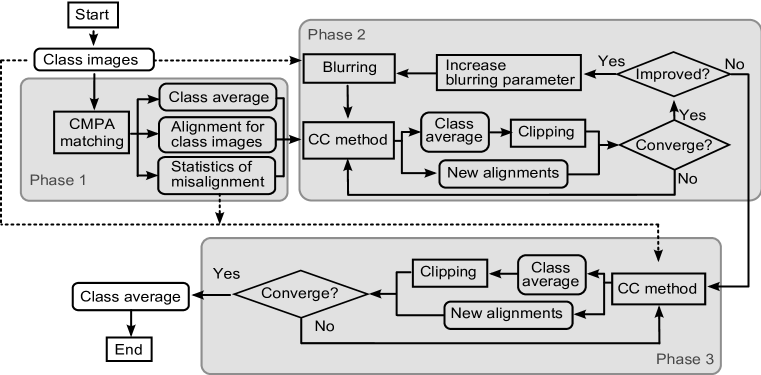
Figure 1: Diagram for the new alignment method.

Figure 2: (a) The original clear projection. (b) The average image with the unattainable perfect alignment for Case 1.

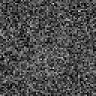
(a) SNR=0.025, $\nu=0$

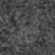
(b) Blurred version of (a)

(c) SNR=0.050, $\nu=0$

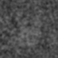
(d) Blurred version of (c)

(e) SNR=0.100, $\nu=0$

(f) Blurred version of (e)

(g) SNR=0.100, $\nu=0.3$

(h) Blurred version of (g)

Figure 3: (a), (c), (e), and (g) Example test images in Case 1,2,3, and 4, respectively. (b), (d), (f), and (h) The blurred version of (a), (c), (e), and (g), respectively. $\nu$ is the correlation between the noise in two adjacent pixels in the background.

	Case 1	Case 2	Case 3	Case 4
SNR	0.025	0.050	0.100	0.100
Correlation	0.0	0.0	0.0	0.3

Table 1: Signal-to-noise ratios and correlations of the adjacent noise pixels for four test cases.

(a) CMPA alignment

(b) #1

(c) #10

(d) #11

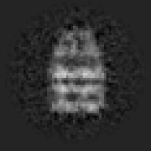
(e) #19

(f) #30

Figure 4: The result of the new method for Case 1. (a) Result by CMPA (Phase 1) (b) Initial image for Phase 2 (c) Result of Phase 2 (d) Initial image for Phase 3 (e) Result of Phase 3 (f) Resulting image after 30 iterations.

(a) Reference 1

(b) Reference 2

(c) Reference 3

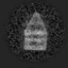
(d) CC 1

(e) CC 2

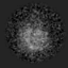
(f) CC 3

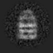
(g) ML 1

(h) ML 2

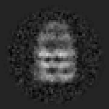
(i) ML 3

Figure 5: The results of the conventional CC and ML methods for Case 1 with three reference images. Reference 3 is one class image.

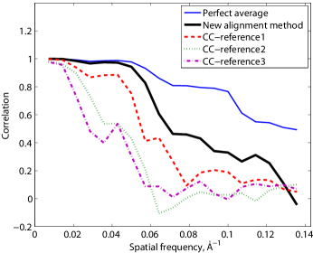
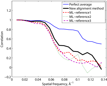
Figure 6: FRC plots for Case 1 (a) Comparison of FRCs of the new method and the CC method (b) Comparison of FRCs of the new method and the ML method

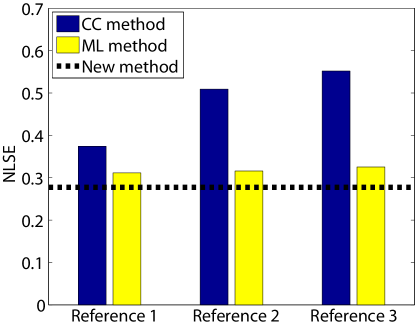
Figure 7: Image difference between the alignment/refinement results and the original image measured by NLSE for Case 1

4 Results

In this section we compute the alignment and the class average for four cases defined in Table 1 using the new method.

To generate the synthetic data images, we first transform (i.e. translate and rotate) the clear projection image shown in Figure 2. The image size is $64\times 64$. The rotational angles are sampled from a uniform distribution on $[0,\,\,2\pi)$. The translation distances are sampled from a Gaussian distribution with the standard deviation, $5$ pixel. This setting is consistent with the assumption in [9]. After transforming, we add noise to the transformed projection. The intensity of the noise is determined so that the resulting image has the SNRs defined in Table 1. The parameter $\nu$ is the correlation coefficient between the noise in adjacent pixels. The method of generating the noise with $\nu$ was introduced in [13]. Figure 2 shows the class average of 500 class images with the perfect alignments for Case 1. Figure 3 shows the noisy data images for the four cases and their blurred version which is used in Phase 2 shown in Figure 1.

The search space for translation is bounded by $(-2.35\xi_{\sigma}\,\,\,2.35\xi_{\sigma})$. Since the probability density function for the rotational angles is bimodal, the two spaces $(-2.35\xi_{\theta},\,\,\,2.35\xi_{\theta})$ and $(-2.35\xi_{\theta}+\pi,\,\,\,2.35\xi_{\theta}+\pi)$ are searched. Note that $\xi_{\sigma}$ and $\xi_{\theta}$ were given in (9) and (10). They are computed from the background noise properties, and are not adjustable parameters. The value 2.35 is the value dictated by Gaussian statistics to guarantee that 98% of the mass under the Gaussian distribution is sampled. The translational misalignment is limited to a multiple of one pixel length because translation by sub-pixel distance involves interpolation and increases the computation time without bringing new information out of images. This limited search also enables us to compute the CC using the DFT. We sample 22 angles for rotational search using the inverse transform sampling. Two sets of 11 samples are drawn from the intervals $(-2.35\xi_{\theta},\,\,\,2.35\xi_{\theta})$ and $(-2.35\xi_{\theta}+\pi,\,\,\,2.35\xi_{\theta}+\pi)$, respectively.

Figure 4(a) shows the coarse alignment obtained by the CMPA match for Case 1. In Phase 2 we use the blurred version of class images to avoid false peaks in the cross correlation. Even though the optimal parameter for the artificial blurring is determined as $\sigma=0.5$ pixel if we apply the full process of Phase 2 described in Section 3.3, we observe that the final result after Phase 3 is not heavily dependent on the blurring parameter as long as we consider $\sigma=0.25,0.50,0.75$ or $1.00$ pixel. For demonstration we fix the standard deviation for the artificial blurring as $\sigma=1$ pixel without losing the benefit of Phase 2. For Case 1, Figure 4(b) shows the first iteration result in Phase 2. And the iteration in Phase 2 was repeated up to 10 iterations (Figure 4(c)). From the $11^{th}$ iteration (Figure 4(d)), Phase 3 is applied until it converges. The $19^{th}$ iteration (Figure 4(e)) shows the converged result. As mentioned earlier, during iterations, the combined transformations for each image are computed and recorded.

Figure 5 shows the results by the CC method and the ML method for Case 1 with three different reference images. For the fair comparison, we use 22 equally-spaced samples on the interval $[0,\,\,\,2\pi)$ for angles in the CC method and the ML method.

Figure 6 shows the Fourier ring correlation (FRC) curves between the pristine projection shown in Figure 2 and resulting images by our new method, the CC method and the ML method. The FRC of the average with perfect alignments shown in Figure 2 is also shown. Figure 7 shows the image differences between the projection shown in Figure 2 and other resulting images by our new method, the CC method and the ML method. The differences are measured using the normalized lease-square error (NLSE). The NLSE of a image $U(m,n)$ relative to another image $V(m,n)$, is defined as

$$\mbox{NLSE}=\sqrt{\frac{\sum^{N}_{m=1}\sum^{N}_{n=1}[U(m,n)-V(m,n)]^{2}}{\sum^{N}_{m=1}\sum^{N}_{n=1}[V(m,n)]^{2}}}.$$

As shown in Figure 6 and 7, the resulting image obtained by our new method is better than the other results. Figure 8-10, 11-12, and 13-14 show the resulting images and their assessment for Case 2,3, and 4, respectively. The resulting images for Case 3 and 4 are not presented since they look similar to the other cases. The assessments for the results are more important and they are provided in Figure 11-14. They consistently show that our new method performs better than existing ones.

When we compute the FRC and the normalized least squared errors, we align two images before computation, because similarity and difference between two images are sensitive to their alignment. Since two images that we compare here are a underlying clear image and a resulting class average by alignment methods, we can apply the cross correlation method to align them without concern about false peaks in cross correlation of noisy images. For more accurate alignment for image comparison, we also apply the image segmentation method to eliminate the area of the residual noise in the class average.

While in Figure 9 the FRC curves of the results of the new method are better than those of the existing methods over all the frequency range, Figure 6 shows that the curve of the result of the new method is lower than the other curves at the highest frequency. This does not mean that the resulting image of the new method is worse than the others, because the curve of the result of the new method is higher at the other frequency and the image difference shown in Figure 7 supports the fact that the new method produces a better image.

In these tests, we used 500 images for one class. The pre-alignment for the 500 images by matching CMPA took approximately 20 seconds using a conventional PC. One iteration in Phase 2 and 3 shown in Figure 1 took about 4.4 seconds. The number of iterations until convergence for each test case is shown in Table 2. One iteration in the classical CC and ML methods takes approximately 2.6 and 6.0 seconds, respectively. The number of iterations until convergence in these existing method are also shown in Table 2. The total computation time of the new method for each case in Table 1 is about 100 seconds, which is the similar computation time of the ML method. The conventional CC method takes about 50 seconds until convergence, but the resulting images are not good as measured using FRC and normalized least squared error. It is important to note that the preprocess to compute or generate a starting reference image for the conventional CC and ML methods is not considered in this computation time. Therefore the total computation time will be increased if that process is included.

	New method	CC 1	CC 2	CC 3	ML 1	ML 2	ML 3
Case 1	19	17	14	20	25	26	25
Case 2	23	11	12	11	27	27	20
Case 3	13	12	19	13	24	21	15
Case 4	17	11	16	10	26	22	28

Table 2: Number of iterations for convergence

Figure 8: The result of the new method for Case 2 (a) CMPA alignment (b) Final result

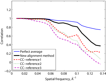
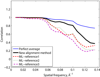
Figure 9: FRC plots for Case 2 (a) Comparison of FRCs of the new method and the CC method (b) Comparison of FRCs of the new method and the ML method

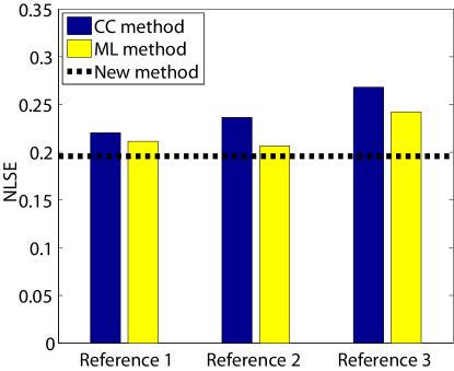
Figure 10: Image difference between the alignment/refinement results and the original image measured by NLSE for Case 2

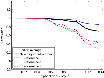
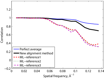
Figure 11: FRC plots for Case 3 (a) Comparison of FRCs of the new method and the CC method (b) Comparison of FRCs of the new method and the ML method

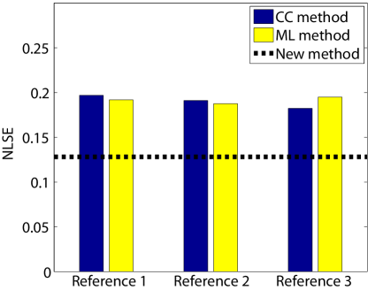
Figure 12: Image difference between the alignment/refinement results and the original image measured by NLSE for Case 3

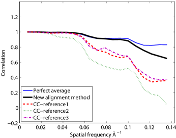
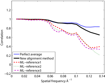
Figure 13: FRC plots for Case 4 (a) Comparison of FRCs of the new method and the CC method (b) Comparison of FRCs of the new method and the ML method

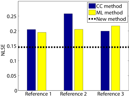
Figure 14: Image difference between the alignment/refinement results and the original image measured by NLSE for Case 4

5 Conclusion

In this work, we developed a new alignment method for class averaging in single particle electron microscopy. The new method consists of two steps: pre-alignment and re-alignment. In the pre-alignment process, images in a class are aligned using their centers of mass and principal axes. Although this pre-alignment does not generate an accurate alignment, it provides a reasonable staring point for the next re-alignment process. Furthermore, we can quantitatively characterize the distribution of misalignments in this pre-alignment method. In the second step, we re-align the images using the results from the first step. Essentially we apply the CC method to re-align images from the first step with the reduced search space that was created based on the statistics of misalignment. In order to avoid problems related to false peaks in the cross correlation, blurred version of the images are used in the first phase of the second step. After iteration with the blurred images, we use the original image to find more accurate alignment.

The pre-alignment step using the CMPA method has several technical benefits. First, it produces a data-driven reference image for the following iteration. Second, the resulting alignment and the corresponding averages are independent of the order of input images unlike the previous work in [6]. Third, it provides the distribution of misalignment regardless of the initial distribution of poses of the projection. In the ML method, the initial distribution of the position of the projection is assumed to be Gaussian, and the orientations are assumed to be uniformly random. What if the initial orientational distributions are different from uniform and how can the distribution be estimated to ensure that this assumption is correct? Our pre-alignment step replaces the pre-existing distribution of the pose of the projection with one that is known. Though the resulting alignment is not perfect, the statistics of misalignment can be quantified and accurately estimated. This misalignment is also independent of the initial distribution of the pose of the projection. Finally, a reduced search space based on the distribution of misalignment can be obtained, and this leads to more accurate alignment.

As we modified the conventional CC method using the CMPA matching and the reduced search space, we can combine the ML method and the CMPA matching method. We expect that the initial estimation for the parameters in (6) is possible. Therefore the iteration in the ML method will converge faster. Technically the distribution function (6) should be modified to reflect that the rotational misalignment after the CMPA matching is no longer uniform. Specifically the function (6) will be a form of (8) and better discretization of integral in (4) based on the new distribution will result in better performance. We leave this work for future research.

References

- [1] S. Ludtke, P. Baldwin, W. Chiu, EMAN: semiautomated software for high-resolution single-particle reconstructions, Journal of Structural Biology 128 (1) (1999) 82–97.
- [2] T. Shaikh, H. Gao, W. Baxter, F. Asturias, N. Boisset, A. Leith, J. Frank, SPIDER image processing for single-particle reconstruction of biological macromolecules from electron micrographs, Nature Protocols 3 (12) (2008) 1941–1974.
- [3] M. Van Heel, G. Harauz, E. Orlova, R. Schmidt, M. Schatz, A new generation of the IMAGIC image processing system, Journal of Structural Biology 116 (1996) 17–24.
- [4] C. Sorzano, R. Marabini, J. Velázquez-Muriel, J. Bilbao-Castro, S. Scheres, J. Carazo, A. Pascual-Montano, XMIPP: a new generation of an open-source image processing package for electron microscopy, Journal of Structural Biology 148 (2) (2004) 194–204.
- [5] J. Frank, Three-dimensional electron microscopy of macromolecular assemblies: visualization of biological molecules in their native state, Oxford University Press, USA, 2006.
- [6] P. Penczek, M. Radermacher, J. Frank, Three-dimensional reconstruction of single particles embedded in ice, Ultramicroscopy 40 (1) (1992) 33–53.
- [7] Z. Yang, P. Penczek, Cryo-EM image alignment based on nonuniform fast Fourier transform, Ultramicroscopy 108 (9) (2008) 959–969.
- [8] L. Joyeux, P. Penczek, Efficiency of 2D alignment methods, Ultramicroscopy 92 (2) (2002) 33–46.
- [9] F. Sigworth, A maximum-likelihood approach to single-particle image refinement, Journal of Structural Biology 122 (3) (1998) 328–339.
- [10] S. Scheres, M. Valle, R. Nuņez, C. Sorzano, R. Marabini, G. Herman, J. Carazo, Maximum-likelihood multi-reference refinement for electron microscopy images, Journal of Molcular Biology 348 (1) (2005) 139–149.
- [11] S. Marco, M. Chagoyen, L. de la Fraga, J. Carazo, J. Carrascosa, A variant to the “random approximation” of the reference-free alignment algorithm, Ultramicroscopy 66 (1-2) (1996) 5–10.
- [12] R. Coifman, Y. Shkolnisky, F. Sigworth, A. Singer, Reference free structure determination through eigenvectors of center of mass operators, Applied and Computational Harmonic Analysis 28 (3) (2010) 296–312.
- [13] W. Park, C. Midgett, D. Madden, G. Chirikjian, A stochastic kinematic model of class averaging in single-particle electron microscopy, International Journal of Robotics Research (accepted).
- [14] G. Chirikjian, Stochastic Models, Information Theory, and Lie Groups, Volume I: Classical Results and Geometric Methods, Birkhauser, 2009.
- [15] G. Jensen, Alignment error envelopes for single particle analysis, Journal of Structural Biology 133 (2-3) (2001) 143–155.
- [16] P. Baldwin, P. Penczek, Estimating alignment errors in sets of 2-D images, Journal of Structural Biology 150 (2) (2005) 211–225.
- [17] W. Park, D. Madden, D. Rockmore, G. Chirikjian, Deblurring of class-averaged images in single-particle electron microscopy, Inverse Problems 26.
- [18] J. Canny, A computational approach to edge detection, IEEE Transactions on Pattern Analysis and Machine Intelligence 8 (6) (1986) 679–698. doi:http://dx.doi.org/10.1109/TPAMI.1986.4767851.
- [19] G. Chirikjian, A. Kyatkin, Engineering Applications of Noncommutative Harmonic Analysis CRC Press, CRC Press, 2001.