Mott insulator dynamics

Abstract

The hydrodynamics of a lattice Bose gas in a time-dependent external potential is studied in a mean-field approximation. The conditions under which a Mott insulating region can melt, and the local density adjust to the new potential, are determined. In the case of a suddenly switched potential, it is found that the Mott insulator stays insulating and the density will not adjust if the switch is too abrupt. This comes about because too rapid currents result in Bloch oscillation-type current reversals. For a stirrer moved through a Mott insulating cloud, it is seen that only if the stirrer starts in a superfluid region and the velocity is comparable to the time scale set by the tunneling, will the Mott insulator be affected.

I Introduction

When Greiner et al. put a system of bosonic atoms in an optical lattice and demonstrated the Mott transition greiner2002 , research on the physics of strongly correlated systems entered a new phase. Cold atoms in optical lattices offer control and detection techniques unthinkable in a condensed matter system. The versatility of optical lattices have teased the imagination of theorists, and copious amounts of papers suggesting exotic types of quantum phase transitions have been published in the past ten years bloch2008 . However, almost all of the suggested quantum phases have proven impossible to realize experimentally at the present for various technical reasons. For example, many rely on spin ordering, which requires temperatures far below what is possible at the present (see, however, the ingenious experiment by Simon et al. using occupation as an effective spin degree of freedom to realize a quantum Ising model simon2011 ).

While the quest for achieving lower temperatures is on ho2007 , there is still lots of interesting science to be done with the relatively simple Bose-Hubbard model on a square lattice. With the possibilities of monitoring directly the local density and low-order correlation functions on the one hand folling2006 ; scherson2010 , and the possibility to manipulate external potentials in real time on the other hand schori2004 , the idea to study the real-time dynamics of a strongly correlated system suggests itself. In particular, these systems are by default trapped in inhomogeneous potentials and therefore they contain finite regions of superfluid and Mott insulator sitting side by side. With current techniques, one can investigate how the interfaces between such regions behave in real time under various kinds of perturbation.

The majority of studies of dynamics of lattice Bose systems have been concerned with quenches clark2004 , Bloch oscillations sachdev2002 , and collective modes in traps pupillo2003 ; lundh2004a ; lundh2004b . These aspects of trapped lattice bosons are by now well understood. Worth mentioning is also an important study of the critical current in interacting lattice Bose systems polkovnikov2005 . Concerning the macroscopic transport of matter and redistribution between quantum phases due to potentials and currents – i.e., the hydrodynamics – the literature is less complete. Natu et al. study the redistribution of matter within an optical lattice following a quench natu2011 . Fischer et al. were concerned with the velocity of a moving superfluid-Mott insulator interface fischer2008 . Karlsson et al. study the behavior of a trapped partly Mott insulating system after turn-off of the trap karlsson2011 , and Snoek and Hofstetter study the dynamics upon displacement of the trap snoek2007 ; this paper will be further discussed below.

The literature survey above indicates that there is need for a more exhaustive understanding of how Mott insulators react to macroscopic currents and potential gradients, which is the subject of this paper. It will provide two sets of numerical examples of how a Bose-Hubbard system containing coexisting Mott and superfluid regions evolves in time following a perturbation in the potential. In order to do this, we evolve the Bose-Hubbard Hamiltonian in time within the mean-field Gutzwiller approximation. In Sec. II the governing equations of motion are put up. In Sec. III, I study the in- and outflow to or from a Mott insulator following the onset of a potential gradient. Sec. IV discusses the perturbation of a Mott insulator using a localized stirrer. In Sec. V I summarize and conclude.

II Lattice Bose gas

We study a system of zero-temperature bosons hopping on a lattice and in addition subject to a more slowly varying external potential. The many-body Bose-Hubbard Hamiltonian is

$$H = -J\sum_{<jj^{\prime}>}\hat{a}^{{\dagger}}_{j}\hat{a}_{j^{\prime}}+\frac{U}{2}\sum_{j}\hat{a}^{{\dagger}}_{j}\hat{a}^{{\dagger}}_{j}\hat{a}_{j}\hat{a}_{j}$$ (1)

$$+ \sum_{j}(V(r_{j})-\mu)\hat{a}^{{\dagger}}_{j}\hat{a}_{j}.$$

Here, $J$ is the tunneling matrix element, $U$ is the interaction parameter and $\mu$ is the chemical potential. $V(r_{j})$ is the external potential and the index $j$ runs over the lattice sites. $r_{j}$ is the spatial coordinate of the $j$:th lattice site. The sum subscripted $<j,j^{\prime}>$ runs over nearest neighbors. We work in units in which $\hbar=1$ and the lattice constant is also unity; hence, both frequencies and velocities can be measured in units of $U$. This paper will be concerned with a two-dimensional square lattice. However, note that the mean-field approximation that will be used here is most accurate in higher dimensions, so the results obtained are best seen as qualitatively describing 3D physics.

The Gutzwiller approximation is based on a mean-field ansatz for the many-body state jaksch1998 ,

$$|\psi_{G}(t)\rangle=\prod_{j}|\phi_{j}(t)\rangle.$$ (2)

In the numerical computations, the on-site states are expanded in a local Fock basis with an upper cutoff $n_{\rm max}$,

$$|\phi_{j}(t)\rangle=\sum_{n=0}^{n_{\rm max}}C_{j,n}(t)|n\rangle_{r}.$$ (3)

In order to calculate the ground state, the Hamiltonian (1) is minimized with respect to the complex coefficients $C_{j,n}$. The time development is obtained by propagating the coupled equations of motion zakrzewski2005 ; schiro2011 ; wernsdorfer2010 ; polkovnikov2005 ; natu2011

$$i\frac{\partial C_{j,n}}{\partial t}=\frac{\partial}{\partial C_{j,n}^{*}}\langle\psi_{G}(t)|H|\psi_{G}(t)\rangle.$$ (4)

In order to diagnose the state, the local total density $n_{j}$ and condensate wave function $\Psi_{j}=\langle\hat{a}_{j}\rangle$ are computed. We will characterize the system by studying the behavior of $n_{j}$, the local condensate density $n_{cj}=|\Psi_{j}|^{2}$, and phase $\varphi={\rm arg}\Psi$. Although simplistic and certainly quantitatively inaccurate in low dimensions, I see this mean-field study of the time development as a first study which can later be vindicated or falsified in more accurate simulation schemes.

The phase diagram for the Bose-Hubbard model was discussed in, e.g., Ref. kuhner1998 . The mean-field critical point at $n=1$ in 2D is $t\approx 0.042U$ at $\mu=0.5U$. If the system is in an external potential, the density is usually well modeled by a local-density approximation (LDA), so that alternating superfluid and Mott insulating regions exist alongside each other, determined by the local chemical potential $\mu-V(r)$. The density profile assumes a characteristic wedding-cake structure bergkvist2004 .

III Outflow from a Mott insulator

We consider a 2D system trapped in a harmonic potential,

$$V_{0}(r_{j})=\frac{\omega^{2}}{2}(x_{j}^{2}+y_{j}^{2}),$$ (5)

where the integer coordinates $x_{j}$ and $y_{j}$ run from $-L+1$ to $L$ as $j$ runs from 0 to $4L^{2}-1$. With the choice $J=0.03U$ and $\mu=0.5U$, the system is Mott insulating in the center with a surrounding superfluid shell. The initial condensate density profile, with $L=32$ and $\omega=0.07U$, is graphed in Figure 1(a).

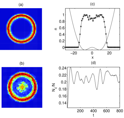
Figure 1: [Color online] Time development of a 2D lattice Bose gas following the turn-on of a wide Gaussian perturbation potential. (a) Spatial distribution of the condensate density before the switch of the potential. (b) Final condensate density, after an evolution of duration $t=800U^{-1}$. (c) Cross-section of the final total density profile (symbols) and potential profile after the switch (line). (b) Fraction of Bose-Einstein condensed atoms as a function of time. The tunneling matrix element is $J=0.03U$, the trap frequency is $\omega=0.07U$, the chemical potential is $\mu=0.5U$, and the Gaussian potential has width $W=10$ lattice sites and strength $V_{1}=0.5U$.

At time $t=0$, with the system in the ground state of the trap, an additional perturbing potential is suddenly switched on,

$$V(r_{j})=V_{0}(r_{j})+V_{1}e^{-(x_{j}^{2}+y_{j}^{2})/W^{2}}.$$ (6)

The resulting total potential assumes a toroidal form, as can be seen in Fig. 1(c). In the case of Fig. 1 I chose $V_{1}=0.5U$ and $W=10$, to make a relatively wide perturbation. There results a rather violent time development, but over time it is seen that the Mott insulating phase is molten and the system assumes something reminiscent of a steady state; Figs. 1(b)-(c) indicate that apart from the noise induced (which I would like to call thermal noise, although the relation between the current mean-field approximation and a finite-temperature Hubbard model is not at all clear) the final density follows the potential profile, closely approximating the LDA. In Fig. 1(d), the total condensate fraction $N_{c}=\sum_{j}n_{cj}$ is plotted as a function of time. As expected it is increasing as the Mott insulator melts, and the time scale of the process is of the order of $100U^{-1}$ or $10J^{-1}$.

However, the picture is different if the potential is switched to large enough values. In Fig. 2, the final potential strength is now set to the larger value $V_{1}=1.0U$.

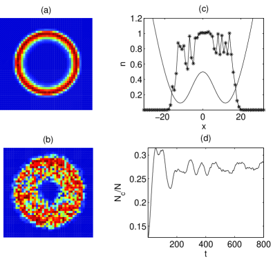
Figure 2: [Color online] Time development of a 2D lattice Bose gas following the turn-on of a wide Gaussian perturbation potential. Panels and parameters are as in Fig. 1, except the height of the Gaussian potential, $V_{1}=1.0U$.

In this case, the Mott insulator resists melting and the system is hindered from approaching equilibrium. A steady state seems to be attained, again after a few inverted hopping periods $J^{-1}$, but it is not the LDA distribution seen in the previous numerical experiment. Figure 2(b-c) show that there is still left a Mott insulating region with unit density at the trap center. In Figure 2(d) we see that in this case, the condensate fraction has also increased a bit, but the important finding is that the central Mott insulator is not entirely molten. This behavior persists over a range of values of the inverted final potential. Further numerical experimentation shows that when $V_{1}$ is larger than about $0.8U$, the Mott insulator insulates.

We have thus found that if the potential is changed a little, the Mott insulator will melt, but if it is changed a lot, it will not. The reason for this behavior becomes clearer if one studies the velocity of the gas. In Fig. 3 the phase of the condensate is plotted for the first numerical experiment.

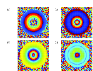
Figure 3: [Color online] Spatial distribution of the condensate phase of a 2D lattice Bose gas in a harmonic trap plus Gaussian potential. Parameters are as in Fig. 1, featuring the weaker Gaussian potential with $V_{1}=0.5U$, and the panels refer to times (a) $t=20U^{-1}$, (b) $t=40U^{-1}$, (c) $t=60U^{-1}$, and (d) $t=100U^{-1}$.

In Fig. 4 it is plotted for the second one.

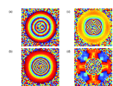
Figure 4: [Color online] Spatial distribution of the condensate phase of a 2D lattice Bose gas in a harmonic trap plus Gaussian potential. Parameters are as in Fig. 2, featuring the stronger Gaussian potential with $V_{1}=1.0U$, and the panels refer to times (a) $t=20U^{-1}$, (b) $t=40U^{-1}$, (c) $t=60U^{-1}$, and (d) $t=100U^{-1}$.

The fluid velocity is related to the wavenumber of the phase variation pattern through the relation $v_{j}=J\sin k_{j}$, where $j=x,y$ denotes a Cartesian coordinate axis. The wavenumbers $k_{j}$ are restricted to lie in the interval $(-\pi,\pi)$. If the potential is steep, the fluid will be accelerated to the maximum wavenumber $\pi$, as is seen to be the case in Fig. 4. This gives rise to a current reversal, which is in essence a Bloch oscillation. At longer times turbulent processes arise, possibly aided by the dynamical instability known to take place in a condensate at $k=\pi/2$ desarlo2005 , and in interacting systems at even smaller wavevectors polkovnikov2005 . The subsequent time development is noisy. This in itself would not necessarily stop the fluid from eventually flowing into the newly created potential wells, and it does not do so if the system is purely superfluid (as seen in simulations not shown here). However, when a Mott insulating region is in the way, the simulations indicate that the whole process is halted and the Mott insulator insulates.

Snoek and Hofstetter snoek2007 studied the dynamics of a trapped lattice boson system following lateral displacement of the trap. Similarly to the present study, they found that Bloch oscillations play a role for the dynamics in the case of large displacements. However, in that study, the system always relaxed towards the new equilibrium in two dimensions. In the present setting, we see that this behavior can be violated.

A wider scan over parameters is collected in Fig. 5.

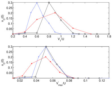
Figure 5: Final central condensate density after the turn-on of a wide Gaussian perturbation potential and subsequent evolution for a duration of $800U^{-1}$. The condensate density $n_{c}$ is averaged over the nine centermost points of the lattice. Plusses denote the result of simulations with a Gaussian perturbation with width $W=10$ and height $V_{1}$; asterisks are for a Gaussian with width $W=15$, and circles are for a Lorenzian profile with width $W=15$. In (a), the x axis is the height of the perturbing potential, $V_{1}$; in (b), it denotes the maximum potential slope, $V^{\prime}_{\rm max}$.

Here, we have measured the condensate density $n_{c}$ in the center at the end of the simulation, and plotted it against the potential height $V_{0}$ as well as against the maximum slope $V^{\prime}_{\rm max}$. Two different Gaussian perturbations are chosen, with widths $W=10$ and $W=15$. In addition, I tried a perturbation with a Lorenzian profile, not because of experimental relevance (it is probably very hard to make), but in order to show that the qualitative result is insensitive to the shape of the potential. It is seen that the core first becomes superfluid when the potential height $V_{1}$ exceeds about 0.4$U$, simply because of LDA considerations. Then, for large enough values of $V_{1}$, there is no superfluid in the core, as we have seen above. This cutoff value depends on the specific potential, as seen in Fig. 5(a), but in Fig. 5(b), the curves collapse onto each other when the condensate density is instead plotted against the maximum potential slope, $V^{\prime}_{\rm max}$, i.e., the maximum potential difference between adjacent sites. The critical value of $V^{\prime}_{\rm max}$ is in this case approximately 0.08$U$, not an integer multiple of $U$, $J$, nor $\omega$, ruling out the simplest guesses for resonance physics, but consistent with the picture that accelerated atoms experience Bloch oscillations.

So far we have only studied a single combination of tunneling strength $J$, trap frequency $\omega$ and chemical potential $\mu$, giving a Mott insulator with $n=1$. Starting in a different Mott insulating region gives the same result, as seen in Fig. 6.

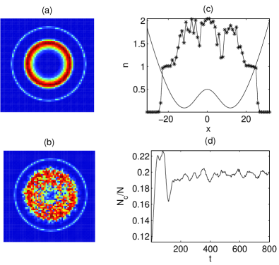
Figure 6: [Color online] Time development of a 2D lattice Bose gas following the turn-on of a wide Gaussian perturbation potential. Panels and parameters are as in Fig. 1, except $J=0.02U$, $\mu=1.5U$, and the height of the Gaussian potential is $V_{1}=1.0U$.

Here, the parameters are chosen as $J=0.02U$, $\mu=1.5U$, and $V_{1}=1.0U$. This means that the central region in the initial state is a $n=2$ Mott insulator surrounded by three shells of alternating superfluid and Mott insulator. Numerical experimentation shows the same behavior as reported above: For a weak enough potential, the central Mott insulator is molten, but for a stronger one it is not.

More curious behavior is seen in a system with a superfluid region in the center. We choose $J=0.3U$, $\mu=1.0U$, and $V_{1}=1.5U$ to produce Fig. 7.

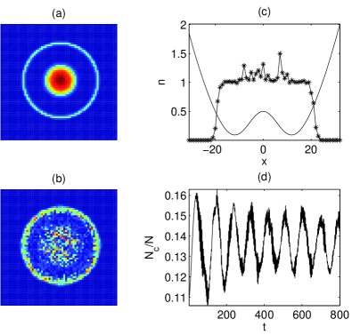
Figure 7: [Color online] Time development of a 2D lattice Bose gas following the turn-on of a wide Gaussian perturbation potential. Panels and parameters are as in Fig. 1, except $J=0.02U$, $\mu=1.0U$, and the height of the Gaussian potential is $V_{1}=1.5U$.

As the peaked potential rises in the center, bosons are flowing out from the central superfluid and finally into the outermost superfluid shell. However, a partly Mott insulating region is left in the center, with a few superfluid atoms intermixed, and then, subsequent dynamics is halted. It is seen in Fig. 7 that the final steady state does not rhyme very well with the applied potential. A closer look at the time dependence is given in Fig. 8.

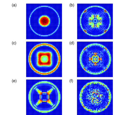
Figure 8: [Color online] Spatial distribution of the condensate density $n_{C}$ of a 2D lattice Bose gas in a harmonic trap plus Gaussian potential. Parameters are as in Fig. 7, featuring several superfluid and Mott insulating shells, and the panels refer to times (a) $t=0U^{-1}$, (b) $t=30U^{-1}$, (c) $t=60U^{-1}$, (d) $t=90U^{-1}$, (e) $t=120U^{-1}$, and (f) $t=600U^{-1}$.

It is seen that the superfluid atoms flow out by creating four jets through the Mott insulator, following the spatial symmetry of the lattice. A noisy state is left behind, containing a small amount of condensate, but as seen above, the final steady state clearly violates the LDA. In this case, it appears that the outflowing superfluid bosons leave a Mott insulator behind; however, a quantitative explanation seems to be out of reach at the present.

IV Stirring a Mott insulator

Now let us investigate what it takes to make a hole in a Mott insulator. To this end, we take a system with $\mu=0.5$ as above; as we have seen this gives a Mott insulator in the center with an approximate width of 20 lattice sites. We move a narrow Gaussian “spoon” potential through the cloud, as was done in Ref. raman2001 to excite vortex pairs in a BEC (cf. lundh2003 ). To produce a reasonably narrow and strong stirrer I choose the parameters $W=3$ and $V_{1}=5.0U$, and the center of the potential moves linearly through the cloud with a velocity $v$,

$$V(r_{j},t)=V_{0}(r_{j})+V_{1}e^{-((x_{j}-vt)^{2}+y_{j}^{2})/W^{2}}.$$ (7)

First, we conclude that a Mott insulator will not be perturbed unless the spoon starts in a superfluid region. This is in accordance with the definition of Mott insulator, and a series of numerical experiments (not shown here) have confirmed this. Thus, we start the spoon at the edge of the simulation cell and move it through the superfluid shell and then to the Mott insulating interior of the cloud.

Figure 9 shows what happens when the spoon is moved quickly through the cloud: The Mott insulator insulates, and the presence of the spoon is only felt as it passes through the thin superfluid shell.

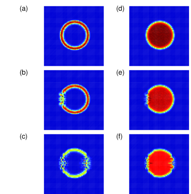
Figure 9: [Color online] Time development of a 2D lattice Bose gas as a Gaussian “spoon” potential is moved through it. The potential has width $W=3$, amplitude $V_{1}=5U$, and velocity $v=0.5U$. The remaining parameters are as in Fig. 1.

In this simulation we chose a velocity $v=0.5U$ (recall that $\hbar=1$ and the lattice constant is 1). This is, in fact, too fast for the tunneling dynamics to respond; in order to melt the insulator one needs to move across a lattice site at a time scale comparable with $J^{-1}$. Such a case is shown in Figure 10, where $v=0.025U$.

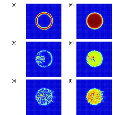
Figure 10: [Color online] As in Fig. 9, but with velocity $v=0.025U$.

Here we see how the spoon, given enough time, excites bosons out of the Mott insulator and depletes the density in the vicinity. An attempt to quantify this result is made in Fig. 11.

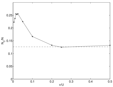
Figure 11: Fraction of Bose-Einstein condensed atoms at the end of a sweep with a Gaussian “spoon” potential, as a function of the velocity with which the spoon is moved. Dashed line: Initial condensate fraction.

Here, we measure the fraction of condensed atoms $N_{c}/N$ at the final time, when the spoon has traversed the entire simulation cell with the length of 64 sites. It is seen that the upper critical velocity for exciting atoms into the condensate is around $v=0.1U$, which is comparable to the tunneling $J$. We note that the sound velocity is likewise of order $J$. These simulation results indicate that making a hole in the Mott insulator is basically a question of moving slow enough, or else the Mott insulator will not budge. When the velocity is decreased below the tunneling strength, though, the curve is seen to decrease again. Indeed, it is natural to expect that for a slow enough spoon, the fluid will adjust adiabatically and the perturbation will again be minimized. Thus, in the case of a moving spoon, we have identified three parameter regimes: An adiabatic regime for velocities about an order of magnitude below $J$; a supersonic regime in which the edge superfluid has no time to react; and an intermediate regime in which the spoon is slow enough to excite the Mott insulating atoms and fast enough to do maximum damage.

V Conclusion

In summary, I have studied the hydrodynamic behavior of a system of lattice bosons in an external potential, by means of a number of numerical experiments. In the first set of experiments, the time development is monitored after a sudden switch of the potential. It is found that if the potential is switched by a small enough amount, the bosons will move in order to adjust to the new potential and a Mott insulator may melt. However, if the switch is large enough, the Mott insulator will not give in and the system stays in a metastable configuration. The reason for this behavior is that the supercurrent breaks down in a Bloch oscillation if the potential switch is too large. In the second set of numerical experiments, a “spoon”-type of localized potential is moved through a system containing a Mott insulating region. The Mott insulator is affected by the spoon if is moved at just the right pace, so that the time scale for traversing a lattice site is comparable to the tunneling time scale, $J^{-1}$. For faster spoons, its presence is not felt in the Mott insulator, and for slower spoons, the whole process is adiabatic.

Experimentally, present techniques for in-situ measurement of filling factor folling2006 ; scherson2010 is the most straightforward way of testing the predictions made here. A classic time-of-flight measurement, which in effect can tell the Bose-Einstein condensed fraction of atoms greiner2002 , is also feasible, as can be seen from the plots of said quantity in the figures.

- (1) M. Greiner et al., Nature 415, 39 (2002).
- (2) I. Bloch, J. Dalibard, and W. Zwerger, Rev. Mod. Phys. 80, 885 (2008).
- (3) J. Simon et al., Nature 472, 307 (2011).
- (4) T.-L. Ho and Q. Zhou, Phys. Rev. Lett. 99, 120404 (2007).
- (5) S. Fölling, A. Widera, T. Müller, F. Gerbier, and I. Bloch, Phys. Rev. Lett. 97, 060403 (2006).
- (6) J. F. Sherson et al., Nature 467, 68 (2010).
- (7) C. Schori, T. Stoferle, H. Moritz, M. Köhl, and T. Esslinger, Phys. Rev. Lett. 93, 240402 (2004).
- (8) S. R. Clark and D. Jaksch, Phys. Rev. A 70, 043612 (2004).
- (9) S. Sachdev, K. Sengupta, and S. M. Girvin, Phys. Rev. B 66, 075128 (2002).
- (10) G. Pupillo, E. Tiesinga, and C. J. Williams, Phys. Rev. A 68, 063604 (2003).
- (11) E. Lundh, Phys. Rev. A 70, 033610 (2004).
- (12) E. Lundh, Phys. Rev. A 70, 061602 (2004).
- (13) A. Polkovnikov, E. Altman, E. Demler, B. Halperin, and M.D. Lukin, Phys. Rev. A 71, 063613 (2005).
- (14) S. S. Natu, K. R. A. Hazzard, and E. J. Mueller, Phys. Rev. Lett. 106, 125301 (2011).
- (15) U. R. Fischer, R. Schützhold, and M. Uhlmann, Phys. Rev. A 77, 043615 (2008).
- (16) D. Karlsson, C. Verdozzi, M. M. Odashima, and K. Capelle, EPL (Europhysics Letters) 93, 23003 (2011).
- (17) M. Snoek and W. Hofstetter, Phys. Rev. A 76, 051603 (2007).
- (18) D. Jaksch, C. Bruder, J.I. Cirac, C.W. Gardiner, and P. Zoller, Phys. Rev. Lett. 81, 3108 (1998).
- (19) J. Zakrzewski, Phys. Rev. A 71, 043601 (2005).
- (20) M. Schiró and M. Fabrizio, Phys. Rev. B 83, 165105 (2011).
- (21) J. Wernsdorfer, M. Snoek, and W. Hofstetter, Phys. Rev. A 81, 043620 (2010).
- (22) T. D. Kühner and H. Monien, Phys. Rev. B 58, R14741 (1998).
- (23) S. Bergkvist, P. Henelius, and A. Rosengren, Phys. Rev. A 70, 053601 (2004).
- (24) L. De Sarlo et al., Phys. Rev. A 72, 013603 (2005).
- (25) C. Raman, J.R. Abo-Shaeer, J.M. Vogels, K. Xu, and W. Ketterle, Phys. Rev. Lett. 87, 210402 (2001).
- (26) E. Lundh, J.-P. Martikainen, and K.-A. Suominen, Phys. Rev. A 67, 063604 (2003).