Investigating transition state resonances in the time domain
by means of Bohmian mechanics: The F+HD reaction

Abstract

In this work, we investigate the existence of transition state resonances on atom-diatom reactive collisions from a time-dependent perspective, stressing the role of quantum trajectories as a tool to analyze this phenomenon. As it is shown, when one focusses on the quantum probability current density, new dynamical information about the reactive process can be extracted. In order to detect the effects of the different rotational populations and their dynamics/coherences, we have considered a reduced two-dimensional dynamics obtained from the evolution of a full three-dimensional quantum time-dependent wave packet associated with a particular angle. This reduction procedure provides us with information about the entanglement between the radial degrees of freedom $(r,R)$ and the angular one $(\gamma)$, which can be considered as describing an environment. The combined approach here proposed has been applied to study the F+HD reaction, for which the FH+D product channel exhibits a resonance-mediated dynamics.

1 Introduction

The analysis in the time domain of processes and phenomena that appear in chemical reactions constitutes nowadays a strong field of research both experimentally and theoretically. From the experimental point of view, the femtosecond techniques developed in the 1990s have allowed us to monitor the process step by step, from reactants to products, with an incredibly high resolution. This has lead to an impressive amount of theoretical work based on wave packet (WP) propagation techniques. In general, these studies are aimed at computing very long time series, from which energy/frequency spectra are obtained at a high resolution (the longer the timescale considered, the finer the features one can define in the corresponding energy/frequency spectrum), which are later on compared with the experiment. Within this scenario, little attention is eventually paid to the evolution of the WP itself, apart from the frame-to-frame picture of the process. Not much information is usually extracted from the corresponding probability density, except for where the latter displays maxima or, on the contrary, presents regions of voids (nodal regions).

In order to obtain an alternative description of the dynamics, one can also analyze the quantum probability current density. Usually this quantity is only considered as a quantum flux to determine how much of the probability density flows into or out a certain region of the configuration space defining the system of interest. It also gives us an idea on how the former evolves in time, just as currents or streams allow us to visualize how a river flows along its bed. This additional information has nevertheless not been much exploited in the literature, except for the study of magnetic properties (because of the needs imposed by the nature of the magnetic field, which is sourceless and therefore has to be considered in hydrodynamic terms). In this sense, Bohmian mechanics [1, 2], a reformulation of standard quantum mechanics in terms of trajectories or, equivalently, streamlines, results of much help. This approach enables us to take the analogy of the river further away: the trajectories behave like the paths pursued by some tracer particles that travel with the stream, thus giving us a precise description of the flow dynamics. This information cannot be obtained directly from the quantum probability current density. It provides us with an insight at a local level of the stream, but does not say anything about how a particular point-like particle evolves when it starts from a certain initial position in the corresponding configuration space. Within this approach, quantum trajectories (QTs) or streamlines are mainly obtained through any of two approaches [3]: synthetic [4, 5, 3] and analytic [6, 7]. Within the former, QTs are computed after solving simultaneously the quantum Hamilton-Jacobi equation and the continuity one, while in the latter (used in this work) one starts from Schrödinger’s equation and then the QTs are obtained from the phase of the wave function.

The use of Bohmian mechanics with interpretational purposes can be traced back to 1926, when Madelung [8] tackled the issue of the interpretation of the wave function (in fashion at the time) by reformulating quantum mechanics in hydrodynamic terms. These ideas underwent a rebirth in the 1970s through the works of Bialynicki-Birula [9, 10] and Hirschfelder [11, 12, 13, 14]. Within this hydrodynamical framework, treating the probability density as a quantum fluid, the chemical reactivity of collinear reactions was formerly studied by the end of the 1960s and beginning of the 1970s by McCullough and Wyatt [15, 16, 17]. This can be considered the starting point for the use of this theory in chemical physics, first at an analytic level and then at a synthetic one by Lopreore and Wyatt [4, 5]. In this latter case, it constituted the source from which a series of numerical algorithms aimed at obtaining the evolution of quantum systems were developed, thus leading to the so-called QT methods [3]. In the same direction, more recently Sanz et al. have analyzed [18, 19] the dynamics associated with a prototype of reactants-to-products reaction described by the so-called Müller-Brown potential energy surface (PES) [20]. On the other hand, the QT methodology has also been exploited by different authors [21, 22, 23, 24, 25, 26, 27, 28, 29, 30, 31] to understand the magnetic properties of molecules within a framework that encompasses electronic structure and topology.

Different theoretical methods have been developed in the literature to analyze, to explain and to understand the formation of transition state resonances. One of the reasons for such an interest relies on the crucial role played by these processes as intermediate stages in chemical reaction dynamics and aggregation processes to form atomic clusters. In this sense, the F+HD reaction constitutes a paradigmatic system. This system has been actively investigated in the last decade due to the the observation through molecular beam experiments of a resonance for the reactive channel F+HD $\to$ HF+D [32, 33]. In the differential cross section, this dynamical feature manifests as a sharp variation of the peaks along the forward-backward scattering directions and, in the corresponding integral cross section, as a step-like profile. Quantum mechanical (QM) calculations on the Stark-Werner (SW) ab initio PES [34] showed that those observations are consistent with a resonance-mediated dynamics of the reaction at a collision energy near 0.5 kcal$\cdot$mol^-1 (0.022 eV). In particular, the existence of a resonance with $(v_{\rm FH}=3,v_{\rm HD}=0)$ quantum numbers for the F–H and H–D stretching modes, respectively, located at the transition state region was theoretically proved [32, 33]. On the contrary, the dynamics of the other product channel, F+HD $\to$ FD+H, was found not to display evidences of similar features.

The specific location of this resonant feature, just above the entrance channel, minimizes the number of partial waves contributing to the integral cross section. This also explains why the peak observed is capable to survive to the averaging introduced when all such partial waves are taken into account. In addition, the resonance lies just below the threshold for reaction predicted by classical approaches, as it has been shown by means of quasi-classical trajectory calculations [35, 36]. Although the maximum peak associated with the resonance was not reproduced in those studies, the rotational motion was found to play a significant role in the overall reaction mechanism. Thus, in order to provide a correct description of the dynamics of the F+HD $\to$ FH+D reaction, a complete three-dimensional (3D) QM approach is required [32].

In this work we have carried out a fully converged QM study for a zero total angular momentum ($J=0)$ by means of a 3D time-dependent wave packet (TDWP) method. In an attempt to further investigate the interpretive capabilities of trajectory-based approaches for this kind of reactive processes, a QT method has been employed in combination with the propagated WP. Thus, besides the 3D WP propagation, projections onto specific values of the angular coordinate ($\gamma$) have been considered to run an alternative QT study of the process. The reason to consider the projection-based analysis presented here arises as a way to avoid the complexity of the full 3D QT dynamics at a first stage, attacking the study of the resonance by only considering the QT propagation within the two-dimensional (2D) radial subspace. In spite of its limitations, this 2D dynamical study is shown to be insightful when compared to the corresponding complete 3D TDWP calculations. More specifically, this Bohmian analysis allows us to determine how the energy/probability associated with a particular angle flows and can be related to the resonance.

This work is organized as follows. In Section 2 the theoretical details of the TDWP and QT approaches are explained. Results are shown and discussed in Section 3. Finally, the main conclusions extracted from this work are summarized in Section 4.

2 Theoretical framework

2.1 The WP procedure

The TDWP method has been described before [37], so here we will only describe the main details involved. Accordingly, consider the total Hamiltonian, $H=T+V$, is described in mass-scaled Jacobi coordinates. With this choice, the kinetic energy operator, $T$, for $J=0$ reads as

$$T=-\frac{\hbar^{2}}{2\mu}\left[\frac{\partial^{2}}{\partial R^{2}}+\frac{\partial^{2}}{\partial r^{2}}+\frac{{\bf l}^{2}}{2\mu R^{2}}+\frac{{\bf j}^{2}}{2\mu r^{2}}\right],$$ (1)

where ${\bf l}$ and ${\bf j}$ are the orbital angular and diatomic rotational angular momentum, respectively, and $V(R,r,\hat{\bf R}\cdot\hat{\bf r})$ is the potential energy function, which in this work corresponds to the SW PES [34].

The WP time propagation can be formally expressed as

$$|\phi_{i}(t)\rangle=e^{-i(H-i\epsilon)t/\hbar}|\phi_{i}(0)\rangle.$$ (2)

Here, this propagation is performed using the symmetric split-operator formula [38],

$$e^{-i(H-i\epsilon)\tau/\hbar}=e^{-iV\tau/2\hbar}e^{-i(T-i\epsilon)\tau/\hbar}e^{-iV\tau/2\hbar}+O(\tau^{3}).$$ (3)

In Eq. (2), the initial-state selected WP, $\phi_{i}(0)$, is assumed to be a product state with the form

$$\phi_{i}(0)=G(R)\phi_{vj}(r)Y_{lj}^{JM}(\hat{\bf R},\hat{\bf r}),$$ (4)

where $G(R)$ is the localized translational wave function, $\phi_{vj}(r)$ is the rovibrational wave function for the selected initial HD state, and

$$Y_{lj}^{JM}(\hat{\bf R},\hat{\bf r})=\sum_{m_{l},m_{j}}\langle lm_{l},jm_{j}|JM\rangle Y_{lm_{l}}(\hat{\bf R})Y_{jm_{j}}(\hat{\bf r})$$ (5)

is a bipolar harmonic. The translational wave function $G(R)$ is given by a Gaussian WP of width $\Delta R_{0}$ and average incident momentum $\hbar k_{0}$, i.e.,

$$G(R)=e^{-(R-R_{0})^{2}/2\Delta R^{2}_{0}-ik_{0}R}.$$ (6)

As it is explained in Ref. [37], a discrete variable representation is employed to describe the radial $R$ and $r$ coordinates, while a basis set of bipolar harmonics is chosen for the angular degree of freedom, $\gamma$. For asymmetric reactions, as in the case considered here, $\gamma$ defines separate regions that correspond to two different product arrangements [37]. In order to avoid numerical reflections as the WP propagates along the different channels associated with the reaction, absorption of the corresponding outgoing probability fluxes is also considered. In this regard, for the absorbing potential $-i\epsilon(R,r)=i\epsilon_{R}(R)-i\epsilon_{r}(r)$ in Eq. (2), we have used the expression proposed in Ref. [37] for the potential originally developed by Manolopoulos [39]. This is applied at $r_{1}$ and $R_{1}$, specific values at the end of the corresponding grids.

The values for the parameters used in the TDWP calculation throughout this work, such as parameters for the initial WP (the center $R_{0}$ of the Gaussian function $G(R)$, the incident wave vector $k_{0}$, and the width $\Delta R_{0}$), the time step ($\tau$), the total propagation time ($t_{tot}$), the maximum value of diatom rotational states ($j_{max}$), the step for the radial grids ($\delta r$ and $\delta R$) and the position of the absorbing potential for the radial coordinates ($R_{1}$ and $r_{1}$) are given in Table 1.

2.2 A brief account on Bohmian mechanics

Consider a system of mass $m$ in Cartesian coordinates. In Bohmian mechanics, the wave function $\Psi$ associated with this system provides us with dynamical information about it at any point on configuration space and any time. More specifically, this information is encoded in the phase of $\Psi$, as infers from the transformation relation

$$\Psi({\bf r},t)=\rho^{1/2}({\bf r},t)e^{iS({\bf r},t)/\hbar},$$ (7)

where $\rho$ and $S$ are the probability density and phase of $\Psi$, respectively, both being real-valued functions. From Eq. (7), Schrödinger’s equation,

$$i\hbar\ \frac{\partial\Psi}{\partial t}=\left(-\frac{\hbar^{2}}{2m}\ \nabla^{2}+V\right)\Psi,$$ (8)

is recast as a system of two real coupled equations,

$$\frac{\partial\rho}{\partial t} + \nabla\cdot\left(\rho\ \frac{\nabla S}{m}\right)=0,$$ (9)

$$\frac{\partial S}{\partial t} + \frac{(\nabla S)^{2}}{2m}+V+Q=0,$$ (10)

where

$$Q\equiv-\frac{\hbar^{2}}{2m}\frac{\nabla^{2}\rho^{1/2}}{\rho^{1/2}}=\frac{\hbar^{2}}{4m}\left[\frac{1}{2}\left(\frac{\nabla\rho}{\rho}\right)^{2}-\frac{\nabla^{2}\rho}{\rho}\right]$$ (11)

is the so-called quantum potential. Equation (9) is the continuity equation, which rules the ensemble dynamics of a swarm of trajectories with initial positions distributed according to $\rho_{0}$; Eq. (10) is the quantum Hamilton-Jacobi equation, which describes the phase field evolution ruling the motion of quantum particles through the motion equation

$${\bf v}=\dot{\bf r}=\frac{\nabla S}{m}.$$ (12)

The coupling between Eqs. (9) and (10) through $Q$ (or, equivalently, $\rho$) is the reason why quantum (Bohmian) dynamics is very different from its classical counterpart, where both equations are only coupled through $S$. This therefore constitutes a very important difference between the typical calculations based on classical trajectories, commonly used in chemical reactivity, although they cannot reproduce quantum features such as tunneling or interference, and simulations based on Bohmian trajectories. In other words, this coupling is precisely the way how the wave function guides the motion of the particle and hence allows QTs to display true quantum features.

Table 1: Parameters used in the TDWP calculations carried out here (see text for details).

Parameter	Value
$R_{0}$ (bohr)	9.6
$k_{0}$ (bohr-1)	0.42
$\Delta R_{0}$ (bohr)	0.09
$\tau$ (fs)	0.016
$t_{tot}$ (fs)	165
$j_{max}$	95
$\delta R$ (bohr)	0.061
$\delta r$ (bohr)	0.052
$R_{1}$ (bohr)	11.0
$r_{1}$ (bohr)	8.0

If instead of trajectories, we are more interested in looking at the quantum system dynamics as the evolution of a quantum fluid, i.e., in a quantum hydrodynamical view, the magnitudes of interest will be the probability density, $\rho=\Psi^{*}\Psi$, and the probability current density, ${\bf J}=\rho{\bf v}=\rho(\nabla S/m)$, related through the continuity equation (9), as

$$\frac{\partial\rho}{\partial t}=-\nabla\cdot{\bf J}.$$ (13)

Hence, instead of talking about trajectories, one speaks about the conservation of the quantum flow, where the analog of Eq. (10) for ${\bf v}$ is a quantum Euler or Navier-Stokes equation and the solutions of Eq. (12) are regarded as fluid streamlines rather than trajectories. These streamlines are obtained by integrating

$${\bf v}=\dot{\bf r}=\frac{{\bf J}}{\rho},$$ (14)

which is formally equivalent to Eq. (12). Accordingly, these lines would follow the flow described by the quantum (probabilistic) fluid which describes the system.

In this work, we are going to explore the 2D restricted dynamics associated with the subspace ($R,r$) describing the F+HD $\to$ FH+D/FD+H reaction. Assuming the last two terms of the kinetic operator given in Eq. (1) can be considered as a part of some effective potential operator, the motion equations describing the evolution of the corresponding reduced QTs will be

$$\dot{R} = \frac{1}{\mu}\frac{\partial S_{\gamma}}{\partial R},$$ (15)

$$\dot{r} = \frac{1}{\mu}\frac{\partial S_{\gamma}}{\partial r},$$ (16)

where $S_{\gamma}$ is the phase associated with the 2D time-dependent reduced wave function $\phi_{\gamma}(R,r;t)$. This wave function is obtained by projecting of the total 3D wave function written in Eq. (2) onto a given angle $\gamma$. In principle, this projected wave function obeys a continuous, smooth evolution in the reduced subspace and, therefore, one also expects the corresponding reduced QTs to display a continuous evolution. Note that this is somehow equivalent to describe the dynamics associated with an effective Hamiltonian

$$H_{\gamma}=-\frac{\hbar^{2}}{2\mu}\frac{\partial^{2}}{\partial R^{2}}-\frac{\hbar^{2}}{2\mu}\frac{\partial^{2}}{\partial r^{2}}+V_{\rm eff}(R,r;\gamma).$$ (17)

Therefore, although this reduced dynamics does not provide a full picture of the 3D system, as we shall see it results very insightful to understand the mechanism of the resonance process in a simplified manner.

It is interesting to stress here that, due to its dependence on all the remaining values of the angular coordinate, the evolution under the Hamiltonian $H_{\gamma}$ can be understood as affected by a sort of environment coordinate. No reduction of the latter by tracing over the associated full 3D density matrix or by means of related phenomenological reduced model [40, 41] is used.

2.3 Quantum trajectories for a Gaussian WP

One of the relevant aspects of the process concerns the preparation of the initial state, for it will determine the subsequent evolution of the chemical species. In order to render some preliminary light on this issue, here we are going to briefly analyze the evolution of our 2D projected WP. The wave function describing our system’s state is given by the product of a Gaussian WP in the $R$-coordinate and the ground state of the asymptotic potential along the $r$-coordinate. This means that, until the wave function is not well inside the interaction region, we will essentially have a wave function which is a free expanding and onwards propagating Gaussian with basically the same width along $r$. Thus, we can simplify the analysis by only considering the evolution of a Gaussian wave function evolving along the $R$-coordinate for times lesser than the time $t_{int}$ at which the interaction is strong enough as to couple the two radial degrees of freedom and the (rotational) angular ones. In this sense, consider $t\ll t_{int}$. The evolution of (6), when normalized, is then approximately described by

$$G(R,t)=A_{t}e^{-(R-R_{cl})^{2}/4\tilde{\sigma}_{t}\sigma_{0}+ik_{0}(R-R_{cl})+iEt/\hbar}.$$ (18)

where $A_{t}=(2\pi\tilde{\sigma}_{t}^{2})^{-1/4}$ and $\Delta R_{0}=\sqrt{2}\sigma_{0}$. This WP moves along the classical trajectory $R_{cl}=v_{0}t$ (for simplicity, we have assumed a zero value for the initial $R_{cl,0}=0$) and its (complex) spreading with time goes as $\tilde{\sigma}_{t}=\sigma_{0}(1+i\hbar t/2m\sigma_{0}^{2})$. The initial velocity by $v_{0}=\hbar k_{0}/\mu=\langle\hat{p}/\mu\rangle$ and the initial energy by $E=\hbar^{2}k_{0}^{2}/2\mu$. The phase (Bohmian action) corresponding to (18) then reads as

$$S_{G}(R,t) = -\frac{\hbar}{2}\ \!\arctan\left(\frac{\hbar t}{2\mu\sigma_{0}^{2}}\right)+Et$$ (19)

$$+\hbar k_{0}R+\frac{\hbar^{2}t}{8\mu\sigma_{0}^{2}\sigma_{t}^{2}}\ \!(R-R_{cl})^{2},$$

with

$$\sigma_{t}=|\tilde{\sigma}_{t}|=\sigma_{0}\sqrt{1+\left(\frac{\hbar t}{2\mu\sigma_{0}^{2}}\right)^{2}}$$ (20)

being the time-dependent real spreading.

The role of the quantum phase in the reaction dynamics is very important and becomes very apparent through the analysis of QTs. An analysis of the early stages of the reaction results very insightful in order to understand the further time-evolution. As said above, these stages are well described by the Gaussian WP (18). Thus, introducing (19) into (15) and then integrating in time, we find

$$R_{q}(t)=R_{cl}(t)+\frac{\sigma_{t}}{\sigma_{0}}\ R_{q,0},$$ (21)

where $R_{q,0}$ is the initial position of the corresponding trajectory. Notice that, in order to get this result, we have assumed that $\phi_{\gamma}(R,r;t)$ can be considered separable in $G(R,t)$ and another function depending on $r$ at these early stages of the evolution, which also means that

$$r_{q}(t)\approx r_{q,0},$$ (22)

i.e., at short times QTs only evolve along the $R$-coordinate, their position remaining essentially constant along the $r$-coordinate.

In Eq. (21) we clearly distinguish the two contributions ruling the time dependence of $G(R)$. First, a classical drift which makes any QT to move alongside the corresponding classical path. This could be therefore regarded as a Bohmian classicality criterion, to some extent related to Ehrenfest’s theorem (see below). The second contribution is a quantum fluid drift, which comes from the own (quantum) nature of the evolution of $\phi_{\gamma}$ and describes the (free) expansion of the WP with time. Accordingly, QTs will separate among themselves at a nonuniform accelerated rate or velocity,

$$\frac{dR_{q}}{dt}=\frac{\sigma_{0}}{\sigma_{t}}\frac{t}{\tau_{q}^{2}}\ R_{q,0},$$ (23)

with $\tau_{q}\equiv 2\mu\sigma_{0}^{2}/\hbar$. That is, contrary to the classical description, quantum-mechanically free expansion involves a stage of accelerated quantum motion. This means that the classical limit will imply keeping this term relatively small and, therefore, that QTs will be essentially parallel to the classical one, $R_{cl}$, in agreement with Ehrenfest’s theorem.

By inspecting (20), two timescales become apparent [42]. If $t\ll\tau_{q}$, the WP spreading is meaningless ($\sigma_{t}\approx\sigma_{0}$) and QTs are all essentially parallel to $R_{cl}$ (Ehrenfest’s or classical criterion), since $R_{q}(t)\approx R_{q,0}+R_{cl}(t)$. In this case, the classical drift becomes the leading term. As $t$ increases, if Eq. (21) is expanded linearly in time, we start to observe the action of the quantum component of the velocity. This leads to an incipient accelerated motion, which at early stages can be described according to the familiar expression from classical mechanics

$$R_{q}(t)\approx R_{q,0}+v_{0}t+\frac{1}{2}\ a_{q}t^{2},$$ (24)

although the acceleration $a_{q}\equiv R_{q,0}/\tau_{q}^{2}$ here depends on the initial position $R_{q,0}$ —the larger the distance $|R_{q,0}-R_{cl,0}|$, the larger the effects due to this quantum acceleration. As time increases asymptotically ($t\gg\tau_{q}$), we find $\sigma_{t}$ approaches a linear dependence on time and the WP curvature becomes invariant under translations in time (this is the so-called Fraunhofer regime in optics, where phases depend linearly on coordinates). In this case, QTs go as

$$R_{q}(t)\approx\left(v_{0}+\frac{R_{q,0}}{\tau_{q}}\right)t,$$ (25)

i.e., the asymptotic motion is again uniform, but with the important difference that the corresponding (constant) velocity having a component proportional to the initial position of the trajectory. This extra QM component is very important: in the case of diffraction by periodic structures, for example, it is precisely the one associated with the different diffraction channels [43] or with the transfer of crystalline momentum [44, 45].

In terms of the 2D problem, this means that at the first stages of its evolution, $\phi_{\gamma}$ will undergo a kind of hyperbolic expansion along the $R$-coordinate, independent of $r$ (where the trajectories will remain essentially steady) and $\gamma$ (for any angle we will observe a similar behavior initially). Actually, in order to determine the leading dynamics from the initial state (i.e., whether the spreading will dominate over the propagation or vice versa), with the values given in Table 1 we find that the value of the ratio $v_{0}/v_{s}=2k_{0}\sigma_{0}$ [46] is approximately 0.027. This means that the WP (18) will propagate along $R$ much slower than it spreads. Therefore, essentially at least half of it will move backwards and will not contribute to the resonance (in other words, the associated amount of reactants will not be reactive). Once the onwards part of the WP (i.e., that spreading towards smaller values of $R$) starts reaching the transition state region, the approach considered here will not be valid any more (we will be in the regime $t\geq t_{int}$). In this case, it is also possible that, due to reflection or interference [18, 19], some additional portion of reactants will also become inactive, bouncing backwards.

3 Numerical simulations

3.1 The model

In the ($R,r$) subspace, the SW PES [34] employed here to study the F+HD reaction is strongly dependent on the Jacobi angular coordinate, $\gamma$, as can be seen in Fig. 1, where a contour-plot of this PES at three different angles is displayed.

In panel (a), for $\gamma=0^{\circ}$, the entrance F+HD channel leads smoothly to the FD+H product channel which exhibits two separated potential minimum regions, a feature due to the possible atom permutations on the corresponding diatom. As $\gamma$ increases these two regions start to get closer and finally merge on an unique minimum well at $\gamma=90^{\circ}$ (see panel (b)). If we keep increasing the angle, the PES starts to describe the other possible product channel, FH+D. Again, the presence of a significantly large barrier creates two unconnected regions, with the separation getting at its highest for $\gamma=180^{\circ}$ (see panel (c)). These projections of the PES at specific angles reveal that the connection of the separated regions observed for $\gamma=0^{\circ}$ and 180^∘ is in fact only possible via the $\gamma\sim 90^{\circ}$ direction. That means that, whereas this pathway is certainly possible for the 3D evolution of the WP, restrictions are expected for the reduced 2D dynamics of the QTs.

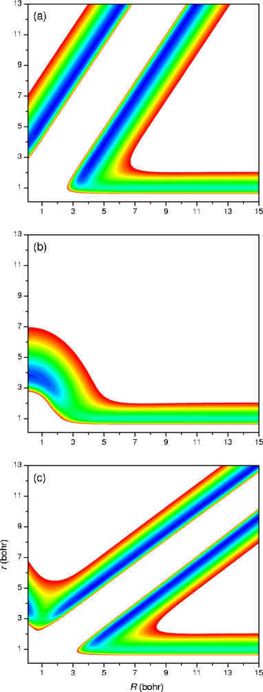
Figure 1: 2D PES (slices) corresponding to the three angles selected here: (a) $\gamma=0^{\circ}$, (b) $\gamma=90^{\circ}$, and (c) $\gamma=180^{\circ}$. Colored contours cover a range of energies between the minimum energy (deep blue), around $-1.5$ eV, and a maximum energy of 3 eV (red).

As mentioned above, the reduced 2D projection is extracted from the 3D WP at each time step $\delta t$ by fixing the angular coordinate, $\gamma$. It is worth noticing that the thus obtained evolution of the 2D WP onto the ($R,r$) subspace will not be equivalent at all (unless the angular degree of freedom is completely decoupled) to the evolution of a strictly 2D WP along any of the potential surfaces displayed in Fig. 1. On the contrary, due to the coupling to the angular coordinate, the 3D WP will lead the evolution of its 2D projection, avoiding motions that one could observe otherwise.

The initial conditions for the corresponding QTs will be chosen taking into account the initial 2D projected probability density at a specific value $\gamma_{0}$ for the angle,

$$\rho_{\gamma_{0}}=|\phi_{\gamma_{0}}(0)|^{2}=|G(R)\phi_{vj}(r)Y_{lj}^{JM}(\gamma_{0})|^{2}.$$ (26)

Although this initial-condition density distribution can be approximated by a Gaussian function in both directions, we have implemented a Monte-Carlo-like distribution based on defining a grid on it and populating each cell according to the corresponding average weight. This procedures renders a fair distribution, as can be seen in Fig. 2, which consists of about 12,800 QTs when we choose a 100$\times$100 grid centered on $\rho_{\gamma_{0}}$ and impose a maximum of 20 trajectories for the maximum value of $\rho_{\gamma_{0}}$. Apart from that, a less fine grid is also chosen to monitor the evolution of relatively large samples of QTs. The center of each cell of this grid is also chosen as the initial condition for a QT, namely the tracer QT, which will help us to understand the coarse grained evolution of the initial WP. In Fig. 2, these tracer trajectories appear as red full circles.

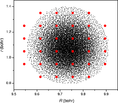
Figure 2: Monte-Carlo-like sampling of the initial conditions for the QTs using the initial probability density. The red bigger dots mark the position of the tracer QTs (see text for details).

Once the initial conditions are set up, QTs are obtained by integrating Eqs. (15) and (16) with the value of the projected 2D WP that we obtained from the propagation from $t$ to $t+\tau$ of the full 3D WP. It is clear that those trajectories approaching the limits of the entrance and exit channels may undergo the effects of the absorption. In principle, one expects that the phase of the guiding wave function will fade gradually and without changing much with respect to the unabsorbed wave function. In order to avoid eventual numerical problems, the evolution of those trajectories that approach the vicinity of the grid boundaries is stopped. That is, each time a QT reaches a maximum value for $R$ and/or $r$, its evolution gets frozen. Note that this procedure is physically reasonable, since any trajectory moving backwards along the F+HD channel or forward along the FD+H or FH+D channels will already be moving asymptotically and, therefore, will not contribute anymore to the reaction dynamics.

3.2 Analysis of WP dynamics and survival probabilities

In order to monitor the formation of the transition state resonance and its survival, as well as the passage to products, when working within the time-dependent domain the most appropriate tool is to define a survival or formation probability [47],

$$\mathcal{P}_{\Sigma}(t)\equiv\int_{\Sigma}\rho_{\gamma_{0}}(t)dRdr.$$ (27)

This quantity gives us the “amount” of probability inside a certain region $\Sigma$ as a function of time. Furthermore, its variation can be used as an indicator of the velocity of the reaction under study. In our case, we can consider the survival probability associated with reactants, products and the transition state resonance. This means that three $\Sigma$ regions have to be defined. For example, looking at Fig. 1(a), the transition state resonance region, $\Sigma_{TSR}$, can be defined as the region enclosing the “elbow” of the PES; the reactants region, $\Sigma_{R}$, as the region enclosing only the entrance F+HD channel; and the products region, $\Sigma_{P}$, as the region above $\Sigma_{TSR}$ (which would include both exit channels).

It is worth mentioning that this approach differs from the spectral quantization analysis performed by Skodje et al. [32]. In that work, the transition state was probed by explicitly setting the initial WP at this region. Here, the survival probabilities are defined in terms of a WP which initiates its evolution from the reactant arrangement.

In Fig. 3 we have plotted the three different probabilities for the three values of $\gamma_{0}$ considered above (see dotted lines). As can be noticed, the two extreme cases ($\gamma_{0}=0^{\circ}$ and $\gamma_{0}=180^{\circ}$) present a certain resemblance: a fast decay of the reactants probability between 30 and 50 fs and an equally fast increase of the products probability, although this happens much earlier and faster along the FH+D channel ($\gamma_{0}=180^{\circ}$). The transition state resonance probability, though, acquires relatively low values. In the case of the T-shape configuration ($\gamma_{0}=90^{\circ}$), the spatial limitations of the PES for the product channels (see Fig. 1(b)) make that all the probability transferred goes to the intermediate resonance region.

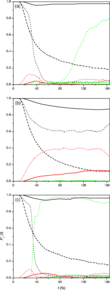
Figure 3: Reactants (black), transition-state (red) and products (green) probabilities as a function of time, obtained from the 2D reduced WP (dotted line), QTs (solid lines) and QTs with absorption (dashed lines). From top to bottom, these probabilities refer to the three different angles considered here: (a) $\gamma_{0}=0^{\circ}$, (b) $\gamma_{0}=90^{\circ}$, and (c) $\gamma_{0}=180^{\circ}$.

The resemblance between the collinear configurations and their difference with respect to the T-shape one can also be seen if we compute the average kinetic energy associated with $\phi_{\gamma_{0}}$,

$$\bar{K}=-\frac{\hbar^{2}}{2m}\ \langle\phi_{\gamma_{0}}(t)|\left(\frac{\partial^{2}}{\partial R^{2}}+\frac{\partial^{2}}{\partial r^{2}}\right)|\phi_{\gamma_{0}}(t)\rangle,$$ (28)

or the squared modulus of its time correlation function,

$$C(t)=|\langle\phi_{\gamma_{0}}(0)|\phi_{\gamma_{0}}(t)\rangle|^{2}.$$ (29)

In Fig. 4 we have plotted these two quantities as a function of time for the three angles considered. As can be seen, in panel (a) we find that $\bar{K}$ increases quickly and then decays more slowly and exponentially for $\gamma_{0}=0^{\circ}$ and 180^∘, while it decreases and becomes almost constant for $\gamma_{0}=90^{\circ}$. Nonetheless, the maximum for $\gamma_{0}=180^{\circ}$ is less pronounced than for $\gamma_{0}=0^{\circ}$, which is connected with the the different dynamics expected for the two possible product arrangements. The existence of a resonance for the F+HD $\to$ FH+D channel leads the WP to stay longer at the spatially confined transition state region, while the unperturbed evolution associated with a direct mechanism that governs the dynamics for the F+HD $\to$ FD+H process. This distinct behavior could account for the larger kinetic energy released for this latter channel. Additional support to this hypothesis will be discussed in the next sections. Regarding $C(t)$, we find a similar trend for the two limiting cases, with an abrupt decay around 30 fs that does not appear for the T-shape configuration.

Figure 4: Average kinetic energy (a) and squared modulus of the time correlation function (b) associated with the reduced 2D wave function $\phi_{\gamma_{0}}$ as a function of time for the three the different angles considered here: $\gamma_{0}=0^{\circ}$ (black), $\gamma_{0}=90^{\circ}$ (red), and $\gamma_{0}=180^{\circ}$ (green).

A similar analysis of survival probabilities can be now carried out in terms of QTs. In this case, the meaning of survival probability becomes closely related, as in classical statistical treatments, to the number of trajectories $N_{\Sigma}$ (each associated with a system configuration) that remain inside the corresponding region at a given time in relation to the total number of trajectories $N$ considered in the statistics [47],

$$\mathcal{W}(t)\equiv\frac{N_{\Sigma}(t)}{N}.$$ (30)

In principle, if the dimensionality of the trajectory-based calculation would be the same as the WP one, $\mathcal{W}$ would approach $\mathcal{P}(t)$ as $N\to\infty$ (given an initial sampling according to $\rho_{0}$). Since this is not the case here for the two simulations performed, $\mathcal{W}$ will give us information about the 2D dynamics, which may differ importantly from the full 3D WP simulation. This is precisely what we observe in Fig. 3 with solid line: a very small portion of the initial configurations sampled will contribute to the resonance and to products, since most of the probability will flow backwards (see next Section). Of course, as some probability is being absorbed, we can also compute $\mathcal{W}$ in terms of a variable total number of trajectories, which gives us the total amount of trajectories that are still inside certain boundaries (see previous Section). However, the corresponding results (dashed lines in Fig. 3) show that the probability mainly concentrates along the reactants regions (indeed, an important portion of it flows backwards, towards large $R$), with no significant contribution from the resonance-forming or the appearance of products processes.

3.3 Analysis of quantum trajectories

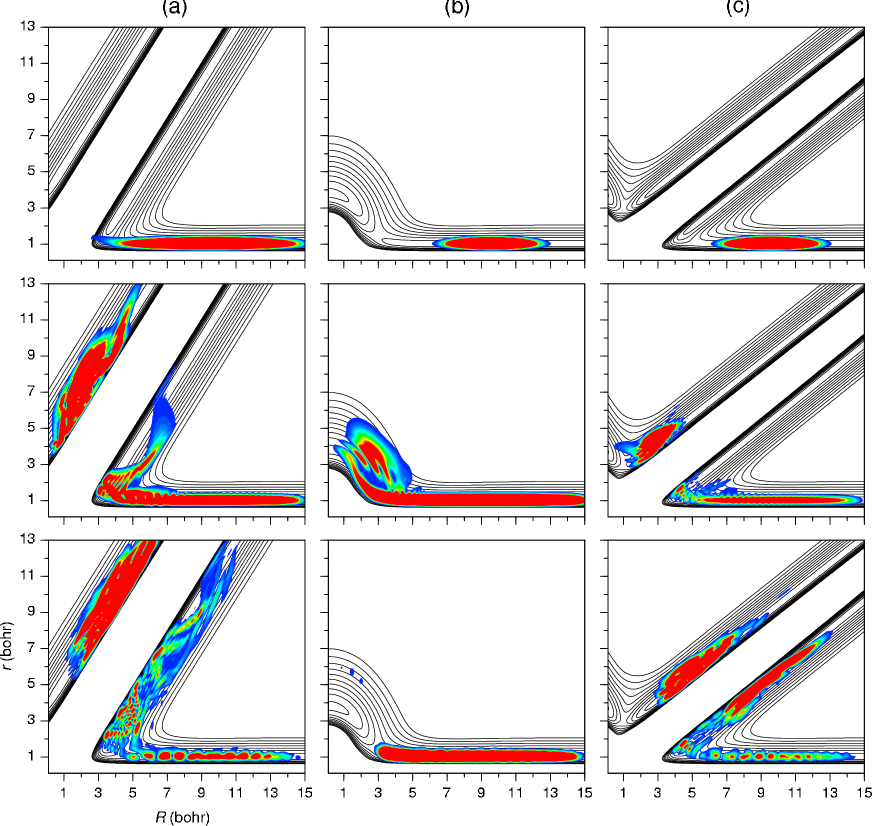
Figure 5: Snapshots illustrating the time-evolution of the reduced 2D WPs corresponding to the three different angles considered here: (a) $\gamma_{0}=0^{\circ}$, (b) $\gamma_{0}=90^{\circ}$, and (c) $\gamma_{0}=180^{\circ}$. From top to bottom, the times associated with each frame of the three cases considered are: (a) 13.2 fs, 39.5 fs, and 72.4 fs; (b) 6.6 fs, 26.3 fs, and 65.8 fs; (c) 6.6 fs, 39.5 fs, and 65.8 fs.

In the previous Section we have analyzed “ensemble” or statistical properties, without paying any attention to the way how the probability flows given a certain angular projection. Thus, let us consider now the evolution of the QTs, in particular the tracer QTs for each one of the angular configurations given above. In this regard, it might be insightful first to consider a few snapshots of the evolution of the reduced 2D WPs for each angle. This is illustrated in Fig. 5.

The evolution for the $\gamma_{0}=0^{\circ}$ case ((a) panels on the left of Fig. 5) shows the WP extending on both branches with a rich nodal structure around the intermediate range. These features though do not seem to remain as the propagation time evolves, thus merely indicating the existence of the expected direct process for the F+HD $\to$ FD+H case. For $\gamma_{0}=90^{\circ}$ ((b) middle panels of Fig. 5), the required bridge between the separated branches shown by the PES at some other angular directions, the WP is restricted to a very localized area at the intermediate region. After spending some time there, a significant component of the WP moves backward into the reactant channel. The situation at $\gamma_{0}=180^{\circ}$ ((c) panels on the right of Fig. 5) clearly reveals the presence of a resonance at the transition state in the FH+D product channel. As the WP reaches the intermediate region a stable 3-node structure is formed, governing the passage to both the upper and lower structures of the exit channels.

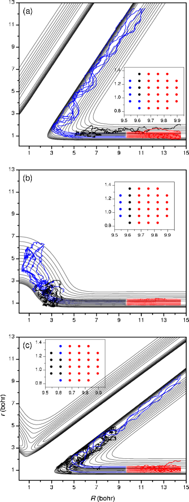
Figure 6: Tracer QTs corresponding to the three different angles considered here: (a) $\gamma_{0}=0^{\circ}$, (b) $\gamma_{0}=90^{\circ}$, and (c) $\gamma_{0}=180^{\circ}$. Non-reactive trajectories are displayed with red color, while reactive ones in (a) and (c) are in blue, as well as those transiently passing to the second channel in (b); with black, tracer QTs that reach the transition state region and then are scattered back. In order to facilitate the identification of the initial conditions leading to each type of motion, they have been plotted in the insets with the corresponding colors.

In Fig. 6 we present the QT counterpart of Fig. 5. The first remarkable feature, as indicated above, is that more than a half of the initial conditions lead to backward motions, this being the cause of the high probability in the reactants region. This justifies the fact of using filtering techniques in order to detect transition state resonances, for the corresponding probability is so small compared to the reactants probability that it would be difficult to detect them otherwise. Now, if we compare the three angular configurations, we readily notice that the number of tracer trajectories remaining in the resonance region (or in a neighborhood) is much larger in the case of $\gamma_{0}=180^{\circ}$ (see panel (c))than for $\gamma_{0}=0^{\circ}$ (panel (a)), where all the trajectories display a direct passage to products. This result is consistent with the features of the resonance observed in the TDWP calculation for $\gamma_{0}=180^{\circ}$ discussed above (see Fig. 5). Moreover, the behavior of the QTs in this particular region, where it is spatially confined, would also support a smaller amount of average kinetic energy as compared with the FD+H channel as commented in the previous section.

On the other hand, in panel (b) we notice that, for the T-shape configuration ($\gamma_{0}=90^{\circ}$), trajectories concentrate for a time around two different regions, which essentially coincide with the separated areas of the FD+H and FH+D channels (see Fig. 1). Furthermore, it is also worth stressing the fact that, since the dynamics is restricted to a 2D plane, the QTs starting in the F+HD channel will only be able to just one of the available regions for the FD+H channel (see panel (a)) or the FH+D one (see panel (c)). The component of the fully 3D WP which explores the upper branch of the PES contours does not manage to carry the corresponding 2D QTs. The trajectory seems to perceive it but not populate it. That is, it is a sort of “empty wave” [2]. In order to make active this part of the wave function, one should consider that initially there is some set of steady initial conditions resting in the associated channel. Then, as this projection of the 3D wave function would start emerging, those initial conditions would start to evolve accordingly.

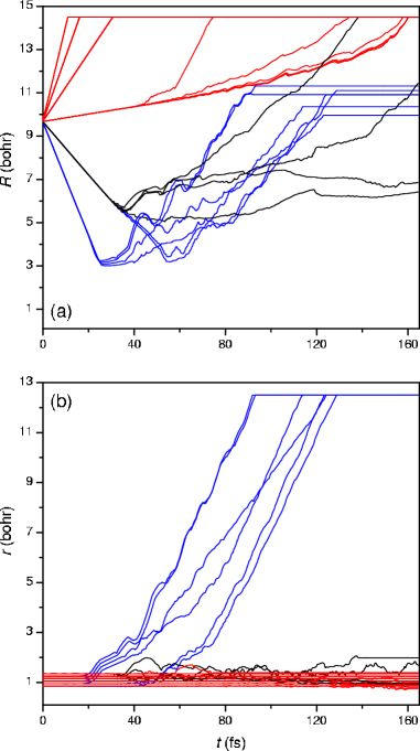
Figure 7: Time-dependence of the $R$ (a) and $r$ (b) degrees of freedom of the tracer QTs corresponding to $\gamma_{0}=0^{\circ}$. Colors are as in Fig. 6.

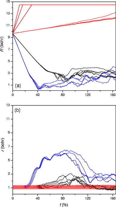
Figure 8: Time-dependence of the $R$ (a) and $r$ (b) degrees of freedom of the tracer QTs corresponding to $\gamma_{0}=90^{\circ}$. Colors are as in Fig. 6.

A complementary picture of the time-evolution of the QTs arises when we look at each degree of freedom separately as a function of time. The corresponding plots are presented in Figs. 7, 8, and 9, respectively. Taking into account this viewpoint, first we notice that for $\gamma_{0}=0^{\circ}$ the $R$-component behaves according to the prescription for a Gaussian WP at early stages of the evolution, as indicated in Section 2.3, while the $r$-component is basically steady (this behavior can also be observed for the other two angular configurations). Then, we find the three well-defined sets of QTs: those moving backwards (red), those moving backwards after reaching the “elbow” of the reduced PES (black), and those passing to products (blue). If we go to $\gamma_{0}=90^{\circ}$ (see Fig. 8), we readily notice the appearance of two groups of trajectories, one exploring the beginning of the upper region observed in both product channels (blue) and another one into the lower structure (black). However, due to the constraint of 2D motion, none of them can indeed penetrate into any of the channels and the trajectories are bounced backwards. Finally, in the case of $\gamma_{0}=180^{\circ}$ (see Fig. 9), we observe a behavior analogous to the one seen for $\gamma_{0}=0^{\circ}$, although now only a smaller portion of the QTs passes to products, the remaining ones keeping trapped around the corresponding PES “elbow” (see Fig. 1(a)).

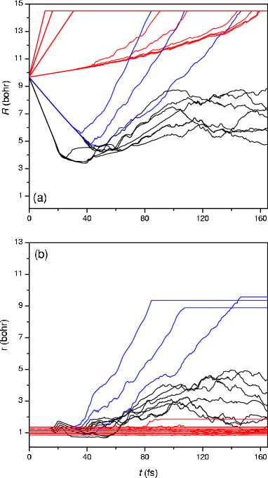
Figure 9: Time-dependence of the $R$ (a) and $r$ (b) degrees of freedom of the tracer QTs corresponding to $\gamma_{0}=180^{\circ}$. Colors are as in Fig. 6.

4 Conclusions

The dynamics of the F+HD reaction for $J=0$ has been investigated by means of a TDWP calculation combined with a QT approach, where the latter was based on computing the trajectories associated with 2D WPs arisen from the projections of the full 3D calculations at given values of the angular coordinate. The evolution of the trajectories has been found to be limited when an explicit angular correlation is required. However, the distinct reaction mechanism for each product channel is successfully described. A clear indication of the resonance-mediated pathway for the FH forming arrangement thus becomes evident within the QT analysis, whereas the 2D evolution of the trajectories for the FD+H product channel is consistent with the observed direct reaction mechanism.

As mentioned in the Introduction, in this work we have focused on the reduced radial subspace in order to avoid the complexity of the full 3D QT dynamics. For the same reason, we have chosen the case $J=0$. This does not mean that the method is limited either theoretically or computationally. Rather it constitutes a firs step in the development of a more general QT methodology aimed at analyzing resonance formation processes. Notice that, by proceeding in this way, one gains an insight on the dynamics that can be later on used to understand in depth the full 3D dynamics. In this regard, if the 2D reduced QT dynamics provides us with interesting information about the flux of probability in these processes for a fixed angle, the 3D dynamics will allow us to understand how this flux is transferred from among different rotational populations. Nevertheless, work in the direction of recreating the full 3D dynamics is currently under development.

References

- [1] D. Bohm, Phys. Rev. 85 (1952) 166; 85 (1952) 180.
- [2] P. R. Holland, The Quantum Theory of Motion, Cambridge University Press, Cambridge, 1993.
- [3] R. E. Wyatt, Quantum Dynamics with Trajectories, Springer, New York, 2005.
- [4] C. L. Lopreore, R. E. Wyatt, Phys. Rev. Lett. 82 (1999) 5190.
- [5] C. L. Lopreore, R. E. Wyatt, Chem. Phys. Lett. 325 (2000) 73.
- [6] R. Guantes, A. S. Sanz, J. Margalef-Roig, S. Miret-Artés, Surf. Sci. Rep. 53 (2004) 199.
- [7] A. S. Sanz, S. Miret-Artés, Phys. Rep. 451 (2007) 37.
- [8] E. Madelung, Z. Phys. 40 (1926) 322.
- [9] I. Bialynicki-Birula and Z. Bialynicka-Birula, Phys. Rev. D 3 (1971) 2410.
- [10] I. Bialynicki-Birula, M. Cieplak, J. Kaminski, Theory of Quanta, Oxford University Press, Oxford, 1992.
- [11] J. O. Hirschfelder, A. C. Christoph, W. E. Palke, J. Chem. Phys. 61 (1974) 5435.
- [12] J. O. Hirschfelder, C. J. Goebel, L. W. Bruch, J. Chem. Phys. 61 (1974) 5456.
- [13] J. O. Hirschfelder, K. T. Tang, J. Chem. Phys. 64 (1976) 760.
- [14] J. O. Hirschfelder, K. T. Tang, J. Chem. Phys. 65 (1976) 470.
- [15] E. A. McCullough, R. E. Wyatt, J. Chem. Phys. 51 (1969) 1253.
- [16] E. A. McCullough, R. E. Wyatt, J. Chem. Phys. 54 (1971) 3578.
- [17] E. A. McCullough, R. E. Wyatt, J. Chem. Phys. 54 (1971) 3592.
- [18] A. S. Sanz, X. Giménez, J. M. Bofill, S. Miret-Artés, Chem. Phys. Lett. 478 (2009) 89.
- [19] A. S. Sanz, X. Giménez, J. M. Bofill, S. Miret-Artés, Chem. Phys. Lett. 488 (2010) 235.
- [20] K. Müller, L. D. Brown, Theor. Chim. Acta 53 (1979) 75.
- [21] R. F. W. Bader, J. Chem. Phys. 73 (1980) 2871.
- [22] J. A. N. F. Gomes, J. Chem. Phys. 78 (1983) 3133.
- [23] J. A. N. F. Gomes, J. Chem. Phys. 78 (1983) 4585.
- [24] P. Lazzeretti, Prog. Nuc. Mag. Res. Spect. 36 (2000) 1.
- [25] S. Pelloni, F. Faglioni, R. Zanasi, P. Lazzeretti, Phys. Rev. A 74 (2006) 012506.
- [26] S. Pelloni, P. Lazzeretti, R. Zanasi, J. Phys. Chem. A 111 (2007) 3110.
- [27] S. Pelloni, P. Lazzeretti, R. Zanasi, Theor. Chem. Acc. 123 (2009) 353.
- [28] S. Pelloni, P. Lazzeretti, J. Phys. Chem. A 112 (2008) 5175.
- [29] S. Pelloni, P. Lazzeretti, J. Chem. Phys. 128 (2008) 194305.
- [30] S. Pelloni, P. Lazzeretti, Chem. Phys. 356 (2009) 153.
- [31] I. García Cuesta, A. Sánchez de Merás, S. Pelloni, P. Lazzeretti, J. Comput. Chem. 30 (2009) 551.
- [32] R. T. Skodje, D. Skouteris, D. E. Manolopoulos, S.-H. Lee, F. Dong, K. Liu J. Chem. Phys. 112 (2000) 4536.
- [33] R. T. Skodje, S. Skouteris, D. E. Manolopoulos, S.-H. Lee, F. Dong, K. Liu Phys. Rev. Lett. 85 (2000) 1206.
- [34] K. Stark, H.-J. Werner, J. Chem. Phys. 104 (1996) 6515.
- [35] F. J. Aoiz, L. Bañares, V. J. Herrero, V. Sáez Rábanos, K. Stark, H.-J. Werner, J. Chem. Phys. 102 (1995) 9248.
- [36] F. J. Aoiz, L. Bañares, V. J. Herrero, V. Sáez Rábanos, K. Stark, I. Tanarro, H.-J. Werner, Chem. Phys. Lett. 262 (1996) 75.
- [37] T. González-Lezana, E. J. Rackham, D. E. Manolopoulos, J. Chem. Phys. 120 (2004) 2247.
- [38] M. D. Feit, J. A. Fleck, Jr., J. Chem. Phys. 78 (1983) 301.
- [39] D. E. Manolopoulos, J. Chem. Phys. 117 (2002) 9552.
- [40] A. S. Sanz, F. Borondo, Eur. Phys. J. D 44 (2007) 319.
- [41] A. S. Sanz, F. Borondo, Chem. Phys. Lett. 478 (2009) 301.
- [42] A. S. Sanz, S. Miret-Artés, Chem. Phys. Lett. 445 (2007) 350.
- [43] A. S. Sanz, S. Miret-Artés, J. Chem. Phys. 126 (2007) 234106.
- [44] A. S. Sanz, F. Borondo, S. Miret-Artés, Phys. Rev. B 61 (2000) 7743.
- [45] A. S. Sanz, F. Borondo, and S. Miret-Artés, Europhys. Lett. 55 (2001) 303.
- [46] A.S. Sanz, S. Miret-Artés, J. Phys. A 41 (2008) 435303.
- [47] A.S. Sanz, S. Miret-Artés, J. Chem. Phys. 122 (2005) 014702.