Non-relativistic bound states in a moving thermal bath

Abstract

We study the propagation of non-relativistic bound states moving at constant velocity across a homogeneous thermal bath and we develop the effective field theory which is relevant in various dynamical regimes. We consider values of the velocity of the bound state ranging from moderate to highly relativistic and temperatures at all relevant scales smaller than the mass of the particles that form the bound state. In particular, we consider two distinct temperature regimes, corresponding to temperatures smaller or higher than the typical momentum transfer in the bound state. For temperatures smaller or of the order of the typical momentum transfer, we restrict our analysis to the simplest system, a hydrogen-like atom. We build the effective theory for this system first considering moderate values of the velocity and then the relativistic case. For large values of the velocity of the bound state, the separation of scales is such that the corresponding effective theory resembles the soft collinear effective theory (SCET). For temperatures larger than the typical momentum transfer we also consider muonic hydrogen propagating in a plasma which contains photons and massless electrons and positrons, so that the system resembles very much a heavy quarkonium in a thermal medium of deconfined quarks and gluons. We study the behavior of the real and imaginary part of the static two-body potential, for various velocities of the bound state, in the hard thermal loop approximation. We find that Landau damping ceases to be the relevant mechanism for dissociation from a certain “critical” velocity on in favor of screening. Our results are relevant for understanding how the properties of heavy quarkonia states produced in the initial fusion of partons in the relativistic collision of heavy ions are affected by the presence of an equilibrated quark-gluon plasma.

I Introduction

When matter is immersed in a thermal medium many of its properties change. In principle, no strictly stationary bound state exists, because interactions with the particles of the medium lead to a finite lifetime for all states (including the ground state). This is equivalent to a broadening of the energy levels, i.e. an imaginary part of the energy eigenvalues, which depends on the density and on the temperature of the medium.

Of particular interest is the case in which the bound state moves with respect to the thermal medium. The first experimental investigations and theoretical developments of this system were done in condensed matter physics cond-mat . From the analysis of atoms moving across a plasma, it has been shown that a number of phenomena may take place. First of all the Debye screening of the Coulomb potential depends on the relative velocity between the bound state and the plasma. Moreover, the propagation of a bound state through the medium produces a fluctuation of the induced potential which leads to a density trail. Finally, the moving particle loses energy and is eventually stopped by the plasma.

A renewed interest in the properties of bound states moving in a thermal medium arose in recent years due to the advent of high energy heavy-ion colliders. In particular, one is interested in understanding whether some modifications of the properties of heavy quarkonia (HQ) states produced in the early stage of the heavy-ion collision can be a signature of the presence of a deconfined plasma of quarks and gluons. In their pioneering work Matsui:1986dk , Matsui and Satz showed that the Debye screening of the color interaction between two static heavy quarks may lead to the dissociation of HQ in a thermal medium. This effect should be experimentally detectable by the suppression of the corresponding yields. The suppression of HQ states means that the yield of HQ observed in heavy-ion collisions is smaller than the yield of HQ one would obtain multiplying HQ production rates in p-p collisions by the number of nucleons participating in the collision and taking into account the normal nuclear absorption; see e.g. Lourenco:2006sr for a brief review. The first study of moving HQ was then performed in Chu:1988wh , in which the dependence of the Debye mass on the velocity of propagation of the heavy quarks with respect to the quark-gluon plasma (QGP) was determined. Subsequent analyses have confirmed the effect and studied the formation of wakes in the QGP Abreu:2007kv ; Mustafa:2004hf ; Ruppert:2005uz ; Chakraborty:2006md ; Chakraborty:2007ug ; Jiang:2010zza .

One may wonder whether the drift of bound states is important, as it is the case for heavy flavors. Indeed, measurements of heavy flavor production in PHENIX Awes:2008qi via single electron measurements results in a large $v_{2}$, which suggest that there is significant damping of heavy quarks while they travel across the fireball. Therefore, in heavy-ion collisions the thermal bath expansion may drift the heavy quarks in a phenomenon similar to advection in normal fluids. This picture has also received support from microscopic calculations of heavy quark diffusion in the quark-gluon plasma vanHees:2007me . However, we expect that the drag of a heavy quarkonium is less important than that of a heavy quark. This is because an isolated heavy quark has a net color charge while a heavy quarkonium at distances larger than its radius is colorless. Hence, in general, we expect that the HQ states produced in the early times of the collision will not be comoving with the thermal medium, and, therefore, our calculations will be relevant for them. On the other hand HQ states produced through recombination are expected to roughly comove with the thermal bath. This is because both heavy quarks have been drifted by the QGP before recombining in a HQ.

Suppression of the J$/\Psi$ was first observed at the CERN SPS Abreu:1997jh . However, in contrast with the naive Debye screening scenario, further experimental investigation of the J$/\Psi$ yields at PHENIX Awes:2008qi , led to the observation of a strong suppression at forward rapidity rather than at mid-rapidity. Recently, there have been efforts in studying this problem with the use of non-relativistic effective field theories (EFTs) Escobedo:2008sy ; Brambilla:2008cx ; Brambilla:2010vq . The EFT techniques are very useful for problems that have different energy scales, as is the case of HQ in a thermal medium. Using these techniques it has been shown that, at least in perturbation theory, the dissociation of bound states is due to the appearance of an imaginary part in the potential Laine:2006ns ; Escobedo:2008sy ; Brambilla:2008cx .

In the present paper we study how a moving thermal bath affects the properties of bound states. One of the points is to assess whether the results obtained in a static medium are modified when considering the relative motion between the bound state and the thermal medium. We consider the simplest systems, hydrogen-like atoms moving at a constant velocity, v, across a homogeneous thermal medium. We study two different cases, the first one corresponds to temperatures smaller or of the order of the typical momentum transfer, the second one corresponds to temperatures larger than the typical momentum transfer. We always assume that the temperature is much smaller than the mass of the particles forming the bound state.

In the first case we restrict ourselves to the hydrogen atom. We consider separately temperatures smaller than the typical momentum transfer and temperatures of the order of the typical momentum transfer. In both temperature ranges we provide the matching procedure and evaluate the energy shifts and decay widths for the stationary states of the system. We build the effective theory for this system first considering moderate values of the velocity and then the relativistic case. We show that for large values of the velocity, a new separation of scale occurs and a different EFT must be constructed for dealing with bound states. In this case the separation of scale is such that the corresponding EFT resembles some aspects of the soft collinear effective theory (SCET) Bauer:2000ew .

In the second case, namely, for temperatures larger than the typical momentum transfer, we also consider muonic hydrogen. Since the mass of the particles forming the bound state is much larger than the mass of the particles in the thermal bath, this system resembles very much a heavy quarkonium in a thermal medium of deconfined quarks and gluons. As a consequence, this part of the present work is of direct relevance for understanding how the properties of heavy quarkonia states produced in the initial fusion of partons in the relativistic collision of heavy ions are affected by the presence of an equilibrated quark-gluon plasma. We study the behavior of the real and imaginary part of the two-body potential for various values of the velocity of the bound state with respect to the thermal bath employing the hard thermal loop (HTL) approximation. Regarding the real part of the potential we reproduce known results, and extend them to higher speeds. The imaginary part of the potential is calculated for the first time. We demonstrate that screening overtakes Landau damping as the dominant mechanism for dissociation at a certain critical velocity.

This paper is organized as follows. In Section II we introduce some general remarks about the propagation of particles in a thermal bath. In Section III and Section IV we study the hydrogen atom moving at moderate velocities and ultrarelativistic velocities with respect to the medium respectively. In Section V we study the real and imaginary part of the static potential of muonic hydrogen in a moving thermal bath for temperatures larger than the typical momentum transfer. The results of this last section are directly applicable to the HQ case. Finally, we present our conclusions in Section VI.

II General framework

In our study we shall employ a reference frame in which the bound state is at rest and the thermal medium moves with a velocity ${\bf v}$. We choose this frame because it facilitates the application of non-relativistic effective field theories, in particular, Non-Relativistic QED Caswell:1985ui (NRQED) and potential NRQED Pineda:1997bj (pNRQED). These EFTs are extremely convenient to handle the three different scales of non-relativistic systems at vanishing temperature Pineda:1997ie ; Pineda:1998kn , and have already proved useful to analyze these systems in a static thermal bath, in which additional scales occur Escobedo:2008sy ; Escobedo:2010tu . They allow one to organize the calculations in such a way that only one scale is taken into account at each step, which, together with the use of dimensional regularization, makes computations much easier.

We shall assume that the plasma (or black-body radiation) is in thermal equilibrium at a temperature $T$. Since we are considering the reference frame in which the plasma is moving with a velocity $\bf v$ the particle distribution functions are given by

$$f(\beta^{\mu}k_{\mu})=\frac{1}{e^{|\beta^{\mu}k_{\mu}|}\pm 1},$$ (1)

where the plus (minus) sign refers to fermions (bosons). In the reference frame where the thermal bath is at rest $\beta^{\mu}k_{\mu}=\frac{k_{0}}{T}$, while in a frame where the plasma moves with a velocity $\bf v$ we have that

$$\beta^{\mu}=\frac{\gamma}{T}(1,{\bf v})=\frac{u^{\mu}}{T}\,,$$ (2)

where $\gamma=1/\sqrt{1-v^{2}}$, $v=|{\bf v}|$, is the Lorentz factor. This frame has been successfully used in the past, for example in Weldon:1982aq . Studying a bound state in a moving thermal bath is akin to study a bound state in non-equilibrium field theory Carrington:1997sq ; in that case the Bose-Einstein or Fermi-Dirac distribution functions are substituted by a general distribution, which in our case will be the boosted Bose-Einstein or Fermi-Dirac distribution functions reported in Eq. (1).

The vector $\bf v$ brings in the problem a number of complications. First of all, it breaks rotational invariance. Second, when $v$ gets close to $1$ new scales are induced, which has serious implications for the use of EFTs. For instance, if we are working with an EFT in which we have integrated out all scales larger than $\mu$, we can no longer argue that if $\mu\gg T$ the Lagrangian of this EFT is not affected by the temperature. This is because the Boltzmann suppression is not only controlled by $T$, but rather is a non-trivial function of $T$ and $\bf v$. In order to illustrate this point, let us analyze the distribution functions in Eq. (1) in more detail.

We begin with a thermal bath consisting of massless particles. Taking into account that in non-equilibrium field theory the collective behavior always enters through on-shell particles or antiparticles, we have (in the case of particles) that

$$\beta^{\mu}k_{\mu}=k\frac{1-v\cos{\theta}}{T\sqrt{1-v^{2}}}\,,$$ (3)

where $k=|{\bf k}|$ and $\theta$ is the angle between $\bf{k}$ and $\bf{v}$. The distribution functions in Eq. (1) can now be written as

$$f(k,T,\theta,v)=\frac{1}{e^{k/T_{\rm eff}(\theta,v)}\pm 1}\,,$$ (4)

where we have defined the effective temperature

$$T_{\rm eff}(\theta,v)=\frac{T\sqrt{1-v^{2}}}{1-v\cos{\theta}}\,.$$ (5)

Intuitively, the dependence of the effective temperature on $v$ and $\theta$ can be understood as a Doppler effect. Indeed Eq. (5) is analogous to the change in the frequency of light caused by the relative motion of the source and the observer. Consider a particle in a thermal bath of radiation moving with velocity $\bf v$. From the point of view of the particle it will see in the forward direction blueshifted radiation and in the backward direction redshifted radiation. This corresponds, respectively, to an effective temperature which is higher in the forward direction than in the backward direction. Therefore, the effective temperature corresponds to the temperature of the radiation as measured by the moving observer and by a minor abuse of language we shall talk about blueshifted and redshifted temperatures. Notice that analogously to the relativistic Doppler effect, the effective temperature in the transverse direction, i.e. in the direction corresponding to $\theta=\pi/2$, is redshifted.

For $v\ll 1$, one has that $T_{\rm eff}(\theta,v)\sim T$ for any value of $\theta$ and one single scale $T$ controls the Boltzmann factor in Eq. (4). However, for $v$ close to $1$, the values of $T_{\rm eff}(\theta,v)$ strongly depend on $\theta$, which gives rise to an interesting case for an EFT analysis. In order to proceed further, it is convenient to use light-cone coordinates. We choose $\bf v$ in the $z$ direction and define

$$k_{+}=k_{0}+k_{3}\qquad{\rm and}\qquad k_{-}=k_{0}-k_{3}\,.$$ (6)

Then, we have that

$$\beta^{\mu}k_{\mu}=\frac{1}{2}\left(\frac{k_{+}}{T_{+}}+\frac{k_{-}}{T_{-}}\right)\,,$$ (7)

where

$$T_{+}=T\sqrt{\frac{1+v}{1-v}}\qquad{\rm and}\qquad T_{-}=T\sqrt{\frac{1-v}{1+v}}\,.$$ (8)

Therefore, in light cone coordinates, it becomes explicit that the distribution function actually depends on two scales, $T_{+}$ and $T_{-}$. For any value of $v$ it is clear that $T_{+}\geq T\geq T_{-}$ and moreover $T_{+}$ correspond to the highest temperature measurable by the observer, while $T_{-}$ corresponds to the lowest temperature measurable by the observer.

For small values of $v$, $T_{+}\simeq T_{-}$ and the shift in the temperature in the forward and backward directions are negligible. In this case no further separation of scale is needed and one has a single temperature scale, $T$, as mentioned before. For $v\simeq 1$, we have $T_{+}\gg T_{-}$, namely, two well separated temperature scales, which must be properly taken into account in our EFTs. Note that configurations with light-cone momenta such that $k_{+}\gg T_{+}$ or $k_{-}\gg T_{-}$ are exponentially suppressed. Then we can separate the remaining configurations in two regions (in light-cone momenta):

• A collinear region, corresponding to $k_{+}\sim T_{+}$ and $k_{-}\lesssim T_{-}$.

• An ultrasoft region, corresponding to $k_{+}\ll T_{+}$ and $k_{-}\lesssim T_{-}$.

The existence of these two regions has to be taken into account in the matching procedure between different EFTs. In this paper we shall analyze two different situations in which $v$ is close to $1$, the case $m_{e}\gg T_{+}\sim 1/r\gg T_{-}\gg E$ and the case $T_{+}\sim m_{e}\gg 1/r\gg T_{-}\gg E$.

We would like to remark that although in Eq. (3) we have assumed for simplicity that the particles of the thermal bath are massless, our approach applies to a plasma that consists of both massless and massive particles. Note that our discussion, from Eq. (6) on, holds independently of what the dispersion relation of the particles in the thermal bath is. If some particles in the plasma have mass $M\gg T$, we know that they are exponentially suppressed in the thermal bath, and this must be true in any reference frame. We can easily verify it by substituting $k_{-}=(M^{2}+{\bf k}^{2}_{\perp})/k_{+}$ in Eq. (7), and by noticing that its minimum is attained at $\beta^{\mu}k_{\mu}=M/T$, which confirms that for $M\gg T$ thermal effects due to these particle can indeed be neglected.

III Hydrogen atom at moderate velocities

In the present section we shall assume that the velocity is moderate, say $v\lesssim 0.5$, so that $T_{+}\simeq T\simeq T_{-}$, and separately study the cases $T\ll 1/r$ and $T\sim 1/r$ ($r$ is the size of the bound state, and hence $1/r$ of the order of the typical momentum transfer). For simplicity, we also assume that the proton is infinitely heavy.

As we have explained in the previous section, in a thermal bath at a temperature $T\ll M$, particles with mass $M$ are exponentially suppressed independently of the value of $v$. In particular, if $M\sim m_{e}$ indicates the mass of electrons and positrons in the plasma, then these particles are irrelevant in our analysis. In this range of temperature the hard thermal loop effects will not appear and the doubling of degrees of freedom plays no role Escobedo:2008sy . This implies that only the transverse photons are sensitive to thermal effects and, hence, the leading order interaction, namely, the Coulomb potential, will not be modified.

III.1 The $T\ll 1/r$ case

As a starting point we consider the pNRQED Lagrangian at vanishing temperature (we use the form given in Eq. (6) of Pineda:1997ie ). We will be able to evaluate the corrections to the binding energy $E_{n}$ and to the decay width $\Gamma_{n}$ due to the thermal bath up to the order $m_{e}\alpha^{5}$. There are two different diagrams that contribute at this order. The first one is the tad-pole diagram which is given by

$$\parbox{113.81102pt}{\includegraphics[scale={0.3}]{./tadus2.eps}}=-\frac{ie^{2}}{m_{e}}\int\frac{\,d^{D}k}{(2\pi)^{D-1}}\frac{\delta(k_{0}^{2}-k^{2})}{e^{|\beta^{\mu}k_{\mu}|}-1}=-\frac{i\pi\alpha T^{2}}{3m_{e}}\,,$$ (9)

where the solid lines represent the atom propagator and the wavy line corresponds to the photon propagator. In the integral we set the number of dimensions $D=4$, because the integral is convergent and $k^{\mu}$ corresponds to the loop momentum. Notice that the contribution of this diagram is independent of $\bf v$ because the loop integral has no indices and no external momentum enters in it. This is in fact true for any tad-pole diagram of this kind. Therefore one can read the result from the ${\bf v}=0$ case Escobedo:2008sy .

Next we consider the “rainbow” diagram,

$$\parbox{113.81102pt}{\includegraphics[scale={0.6}]{./selfus2.eps}}=-\frac{e^{2}}{m_{e}^{2}}\lim_{p_{0}\to E_{n}}\sum_{r}\langle n|p^{i}|r\rangle I_{ij}(p_{0}-E_{r})\langle r|p^{j}|n\rangle\,.$$ (10)

$p^{i}$ is the momentum operator of the electron, $|r\rangle$ symbolizes an eigenstate of the Coulomb Hamiltonian of energy $E_{r}$, and $I_{ij}(q)$ is defined as follows:

$$I_{ij}(q)=\int\frac{\,d^{D}k}{(2\pi)^{D-1}}\frac{\delta(k_{0}^{2}-k^{2})}{e^{|\beta^{\mu}k_{\mu}|}-1}\frac{i}{q-k_{0}+i\epsilon}\left(\delta_{ij}-\frac{k_{i}k_{j}}{k^{2}}\right)\,.$$ (11)

Since the only two independent tensors are $\delta_{ij}$ and $v_{i}v_{j}$, one can use the decomposition

$$I_{ij}=A\,P^{s}_{ij}+B\,P^{p}_{ij}\,,$$ (12)

where

$$P^{s}_{ij}=\frac{1}{2}\left(\delta_{ij}+\frac{v_{i}v_{j}}{v^{2}}\right)\qquad{\rm and}\qquad P^{p}_{ij}=\frac{1}{2}\left(\delta_{ij}-3\frac{v_{i}v_{j}}{v^{2}}\right)\,,$$ (13)

and then

$$A=\frac{1}{2}I_{ii}\qquad{\rm and}\qquad B=\frac{1}{2}\left(I_{ii}-2\frac{v^{i}v^{j}}{v^{2}}I_{ij}\right)\,.$$ (14)

Upon substituting Eq. (11) in the expressions above, we find that

$$A=\int\frac{\,d^{D}k}{(2\pi)^{D}}\frac{\delta(k_{0}^{2}-k^{2})}{e^{|\beta^{\mu}k_{\mu}|}-1}\frac{i}{q-k_{0}+i\epsilon}\qquad{\rm and}\qquad B=\int\frac{\,d^{D}k}{(2\pi)^{D}}\frac{\delta(k_{0}^{2}-k^{2})}{e^{|\beta^{\mu}k_{\mu}|}-1}\frac{i}{q-k_{0}+i\epsilon}\frac{({\bf v}\cdot{\bf k})^{2}}{v^{2}k^{2}}\,.$$ (15)

The computations of these integrals is done in Appendix A. The results for the imaginary and real part of $A$ are, respectively, given by

$$\Im A(q)=\frac{q}{4\pi^{2}}\left(\log\left(\frac{2\pi T}{|q|}\right)+1-\frac{1}{2v}\log\left(\frac{1+v}{1-v}\right)+\frac{\pi T\sqrt{1-v^{2}}}{|q|v}\Im\log\left(\frac{\Gamma\left(\frac{i|q|}{2\pi T_{+}}\right)}{\Gamma\left(\frac{i|q|}{2\pi T_{-}}\right)}\right)\right)$$ (16)

and

$$\Re A(q)=-\frac{T\sqrt{1-v^{2}}}{8\pi v}\log\left(\frac{1-e^{-\frac{|q|}{T_{+}}}}{1-e^{-\frac{|q|}{T_{-}}}}\right)\,.$$ (17)

The imaginary part of $B$ turns out to be given by

$$\Im B(q)=\frac{q}{12\pi^{2}}\left(\log\left(\frac{2\pi T}{|q|}\right)+\frac{1}{3v^{2}}(3+v^{2})-\frac{1}{2v^{3}}\log\left(\frac{1+v}{1-v}\right)+\frac{3}{2}\int_{-1}^{1}\,d\lambda\lambda^{2}\Re\Psi\left(\frac{i|q|(1-v\lambda)}{2\pi T\sqrt{1-v^{2}}}\right)\right)\,,$$ (18)

while for the real part of $B$ we have

$$\Re B(q)=-\frac{T\sqrt{1-v^{2}}}{8\pi v^{3}}\int_{\frac{|q|}{T_{-}}}^{\frac{|q|}{T_{+}}}\,dt\left(1-\frac{T\sqrt{1-v^{2}}t}{|q|}\right)^{2}\frac{1}{e^{t}-1}\,.$$ (19)

The expressions above can be computed numerically for any value of the parameters. The thermal corrections to the energy and the decay width (for arbitrary angular momentum) are given by the following expressions:

$$\delta E_{nlm}=\frac{\alpha\pi T^{2}}{3m}+\frac{e^{2}}{m_{e}^{2}}\lim_{p_{0}\to E_{n}}\sum_{r}\langle n|p^{i}|r\rangle\Im I_{ij}(p_{0}-E_{r})\langle r|p^{j}|n\rangle\,,$$ (20)

and

$$\delta\Gamma_{nlm}=\frac{2e^{2}}{m_{e}^{2}}\lim_{p_{0}\to E_{n}}\sum_{r}\langle n|p^{i}|r\rangle\Re I_{ij}(p_{0}-E_{r})\langle r|p^{j}|n\rangle\,,$$ (21)

which in general will depend on the relative velocity $\bf v$. Analytical expressions for $T\gg E$ and for $T\ll E$, where $E\sim E_{n}$, the binding energy scale, are derived below.

III.1.1 The $T\gg E$ case

For $T\gg E$ the leading contribution to the integrals in Eqs. (16), (17) and Eqs. (18), (19) can be analytically determined and upon substituting the corresponding expressions in $I_{ij}$ we find that

$$\Re I_{ij}=\frac{T\sqrt{1-v^{2}}}{8\pi v}\left(P^{s}_{ij}\log\left(\frac{1+v}{1-v}\right)+P^{p}_{ij}\frac{\log\left(\frac{1+v}{1-v}\right)-2v}{v^{2}}\right)+\mathcal{O}(E)\,,$$ (22)

for the real part of $I_{ij}$ and

$$\Im I_{ij}=\frac{q}{4\pi^{2}}\left[P^{s}_{ij}\left(\log\frac{2\pi T}{|q|}-\frac{1}{2v}\log\left(\frac{1+v}{1-v}\right)+1-\gamma\right)+P^{p}_{ij}\frac{1}{3}\left(\log\frac{2\pi T}{|q|}+\frac{1}{v^{2}}+\frac{1}{3}-\frac{1}{2v^{3}}\log\left(\frac{1+v}{1-v}\right)-\gamma\right)\right]+\mathcal{O}\left(\frac{E^{2}}{T}\right)\,,$$ (23)

for the imaginary part of $I_{ij}$.

It is interesting to observe that, in this limit, the terms non-local in $q$ (Bethe-log type) coincide with those obtained for vanishing velocity. Hence, all dependence on $\bf v$ is encoded in an anisotropic potential and kinetic term. This result will also serve as a cross-check of the $1/r\sim T$ computation that will be carried out in the next section.

In order to obtain the energy shift and the decay width from Eqs. (22) and (23) we consider separately the S-wave states and states with non-vanishing angular momentum. We display below slightly more general results, which hold for an ion of charge $Z$ as well.

In the S-wave states the expected value of any tensor operator $\langle n|O_{ij}|n\rangle\propto\delta_{ij}$, therefore terms proportional to $P^{p}_{ij}$, can be ignored (because $P^{p}_{ij}$ is traceless) and we find that

$$\delta E_{n} = \frac{\alpha\pi T^{2}}{3m_{e}}-\frac{4Z\alpha^{2}}{3}\frac{|\phi_{n}({\bf 0})|^{2}}{m_{e}^{2}}\left(-\frac{1}{2v}\log\left(\frac{1+v}{1-v}\right)+1-\gamma\right)$$ (24)

$$+ \frac{2\alpha}{3\pi m_{e}^{2}}\sum_{r}|\langle n|{\bf p}|r\rangle|^{2}(E_{n}-E_{r})\log\left(\frac{2\pi T}{|E_{n}-E_{r}|}\right),$$

where $\phi_{n}({\bf 0})$ is the wave function at the origin. The corresponding change in the width turns out to be given by

$$\delta\Gamma_{n}=\frac{2Z^{2}\alpha^{3}T\sqrt{1-v^{2}}}{3n^{2}v}\log\left(\frac{1+v}{1-v}\right)\,.$$ (25)

States with non-vanishing angular momentum are more difficult to deal with. It is convenient to decompose $I_{ij}$ by the tensors $\delta_{ij}$ and $\frac{v_{i}v_{j}}{v^{2}}$ instead of $P^{s}_{ij}$ and $P^{p}_{ij}$. For the real and imaginary parts of $I_{ij}$ we find respectively

$$\Re I_{ij}=\frac{T\sqrt{1-v^{2}}}{16\pi v}\left[\delta_{ij}\left(\left(1+\frac{1}{v^{2}}\right)\log\left(\frac{1+v}{1-v}\right)-\frac{2}{v}\right)+\frac{v_{i}v_{j}}{v^{2}}\left(\left(1-\frac{3}{v^{2}}\right)\log\left(\frac{1+v}{1-v}\right)+\frac{6}{v}\right)\right],$$ (26)

and

$$\Im I_{ij} = \frac{q}{4\pi}\left[\frac{2\delta_{ij}}{3}\left(\log\left(\frac{2\pi T}{|q|}\right)-\gamma+\frac{5}{6}+\frac{1}{4v^{2}}-\frac{3}{8v}\left(1+\frac{1}{3v^{2}}\right)\log\left(\frac{1+v}{1-v}\right)\right)-\frac{v_{i}v_{j}}{2v^{2}}\rho(v)\right]\,,$$ (27)

where

$$\rho(v)=\frac{1}{2v}\left(1-\frac{1}{v^{2}}\right)\log\left(\frac{1+v}{1-v}\right)-\frac{2}{3}+\frac{1}{v^{2}}\,.$$ (28)

To determine the energy shifts and the decay widths we fix ${\bf v}$ in the $z$-direction, and make use of the following identities

$$\Bigg{<}n\Bigg{|}\frac{({\bf v}\cdot{\bf p})^{2}}{v^{2}}\Bigg{|}n\Bigg{>}=\langle n|p^{2}|n\rangle\frac{\sqrt{4\pi}}{3}\Bigg{<}Y_{lm}\Bigg{|}\left(Y_{00}+\sqrt{\frac{4}{5}}Y_{20}\right)\Bigg{|}Y_{lm}\Bigg{>}\,,$$ (29)

and

$$\langle n|[[H,{\bf v}\cdot{\bf p}],{\bf v}\cdot{\bf p}]|n\rangle=\sqrt{\frac{4\pi}{5}}Z\alpha\Bigg{<}n\Bigg{|}\frac{1}{r^{3}}\Bigg{|}n\Bigg{>}\langle Y_{lm}|Y_{20}|Y_{lm}\rangle,$$ (30)

where $Y_{lm}$ are the spherical harmonics. Note that $|n\rangle$ is used as a short-hand notation for $|nlm\rangle$, where $n$ is the principal quantum number, $l$ the orbital angular momentum and $m$ its $z$-component. With these expressions we obtain the general forms of the shifts of the energy levels

$$\delta E_{nlm} = \frac{\alpha\pi T^{2}}{3m_{e}}+\frac{2\alpha}{3\pi m_{e}^{2}}\sum_{r}|\langle n|{\bf p}|r\rangle|^{2}(E_{n}-E_{r})\log\left(\frac{-E_{1}}{|E_{n}-E_{r}|}\right)$$ (31)

$$- \frac{Z^{3}\alpha^{2}\langle 2l00|l0\rangle\langle 2l0m|lm\rangle}{2\pi m_{e}^{2}a_{0}^{3}n^{3}l(l+\frac{1}{2})(l+1)}\rho(v)\,,$$

and the corresponding widths are given by

$$\delta\Gamma_{nlm}=\frac{Z^{2}\alpha^{3}T\sqrt{1-v^{2}}}{3n^{2}v}\left(2\log\left(\frac{1+v}{1-v}\right)+\left(\left(1-\frac{3}{v^{2}}\right)\log\left(\frac{1+v}{1-v}\right)+\frac{6}{v}\right)\langle 2l00|l0\rangle\langle 2l0m|lm\rangle\right)\,,$$ (32)

where $\langle lml^{\prime}m^{\prime}|l^{\prime\prime}m^{\prime\prime}\rangle$ are the Glebsch-Gordan coefficients (normalization and sign conventions are as in Sakurai ).

It is interesting to observe that the decay widths (25) and (32) decrease as the velocity increases.

III.1.2 The $T\ll E$ case

For temperatures $T\ll E$ the coefficients $A$ and $B$ simplify and upon replacing their expressions in Eq. (12) we obtain that

$$I_{ij}(q)=\frac{iT^{2}(1-v^{2})}{32q}\int_{-1}^{1}\frac{\,d\lambda}{(1-v\lambda)^{2}}\left(P_{ij}^{s}+\lambda^{2}P_{ij}^{p}\right)+\mathcal{O}\left(\frac{T^{4}}{q^{3}}\right)\,.$$ (33)

When this expression is used in the evaluation of the energy shift in Eq. (20) and of the decay width in Eq. (21), we need to calculate

$$P_{ij}^{x}\sum_{r}\langle n|p^{i}|r\rangle\frac{1}{E_{n}-E_{r}}\langle r|p^{j}|n\rangle=-{m_{e}\over 2}P_{ii}^{x}\,,$$ (34)

for $x=s,p$. Note that only the term proportional to $P_{ij}^{s}$ contributes because $P_{ij}^{p}$ is traceless. Thus, the contribution from the rainbow diagram in the limit $T\ll E$ for states with vanishing angular momentum is given by

$$\parbox{113.81102pt}{\includegraphics[scale={0.3}]{./selfus.eps}}=\frac{i\pi\alpha T^{2}}{3m_{e}}+\mathcal{O}\left(\frac{\alpha^{3}T^{4}}{E^{3}}\right)\,,$$ (35)

and is independent of the velocity $v$. Hence, the dominant contribution of the rainbow diagram above cancels the contribution of the tad-pole diagram, which we have seen to be independent of $v$ as well. Then the thermal corrections in this case are very suppressed, of the order ${\cal O}(\alpha^{3}T^{4}/E^{3})$, like in the case of the thermal bath at rest.

III.2 The $T\sim 1/r$ case

In the temperature regime $T\sim 1/r$, the temperature is high enough so that its effects must be taken into account already in the matching between NRQED and pNRQED, namely it affects the potential. Therefore, several diagrams are modified by the presence of the temperature. However, like in the calculations for the thermal bath at rest, there are only four diagrams that give a relevant contribution. All other diagrams give contributions that either vanish or can be shown to cancel out by local field redefinitions. We schematically analyze the relevant diagrams below. Then, as a cross check, we compare the calculations for $T\sim 1/r$ in the limit of low temperature, with the results that we derived in the previous section for $E\sim T$ in the limit of high temperature, and we find agreement.

The four diagrams that must be taken into account in the matching procedure between NRQED and pNRQED are the following:

• The tad-pole diagram which comes from the $\frac{D^{2}}{2m_{e}}$ term in the NRQED Lagrangian and gives the contribution

  $$\parbox{113.81102pt}{\includegraphics[scale={0.3}]{./tadus.eps}}=-\frac{i\pi\alpha T^{2}}{3m_{e}}\,.$$ (36)

  This diagram is quite similar to the diagram we evaluated in the previous section, but now the solid line corresponds to the electron field instead of the hydrogen atom. As already discussed, this diagram is independent of the velocity $v$.

• The rainbow diagram is given by

  $$= -\frac{-ie^{2}p^{i}p^{j}}{2m_{e}^{2}}\int\frac{\,d^{D-1}k}{(2\pi)^{D-1}k}\frac{1}{e^{\frac{k}{T\sqrt{1-v^{2}}}(1-\frac{{\bf v}\cdot{\bf k}}{k})}-1}\left(\delta_{ij}-\frac{k_{i}k_{j}}{k^{2}}\right)$$

  $$\times \left(\frac{1}{p_{0}-k-\frac{({\bf p}-{\bf k})^{2}}{2m_{e}}}+\frac{1}{p_{0}+k-\frac{({\bf p}+{\bf k})^{2}}{2m_{e}}}\right)\,,$$

  where the solid line corresponds to the electron field and the wavy line corresponds to the photon. In order to have a consistent EFT we have to expand

  $$\frac{1}{p_{0}-k-\frac{({\bf p}-{\bf k})^{2}}{2m_{e}}}+\frac{1}{p_{0}+k-\frac{({\bf p}+{\bf k})^{2}}{2m_{e}}}\to-2\frac{p_{0}-\frac{p^{2}}{2m_{e}}}{k^{2}}-\frac{1}{m_{e}}\,,$$ (38)

  and therefore the contribution of the rainbow diagram can be written as

  $$\parbox{113.81102pt}{\includegraphics[scale={0.3}]{./selfus.eps}}=\left(p_{0}-\frac{p^{2}}{2m_{e}}\right)\frac{ie^{2}p^{i}p^{j}}{m_{e}^{2}}T_{ij}+\frac{ie^{2}}{2m_{e}^{3}}p^{i}p^{j}R_{ij}\,,$$ (39)

  where

  $$T_{ij}=\int\frac{\,d^{D-1}k}{(2\pi)^{D-1}k^{3}}\frac{1}{e^{\frac{k}{T\sqrt{1-v^{2}}}(1-\frac{{\bf v}\cdot{\bf k}}{k})}-1}\left(\delta_{ij}-\frac{k_{i}k_{j}}{k^{2}}\right)\,,$$ (40)

  and

  $$R_{ij}=\int\frac{\,d^{D-1}k}{(2\pi)^{D-1}k}\frac{1}{e^{\frac{k}{T\sqrt{1-v^{2}}}(1-\frac{{\bf v}\cdot{\bf k}}{k})}-1}\left(\delta_{ij}-\frac{k_{i}k_{j}}{k^{2}}\right)\,.$$ (41)

  For the time being we do not evaluate these integrals; as we shall clarify soon we only need to evaluate $T_{ij}$.

• The thermal correction of the Coulomb potential corresponds to the diagram

  $$\parbox{113.81102pt}{\includegraphics[scale={0.3}]{./rdcoulomb.eps}}=\frac{ie^{4}p^{i}{p^{\prime}}^{j}}{m_{e}^{2}|{\bf p}-{\bf p}^{\prime}|^{2}}T_{ij}\,,$$ (42)

  where the tensor $T_{ij}$ is the same as in Eq. (40) and $\bf p$ and $\bf p^{\prime}$ are the momenta of the incoming and outgoing electrons, respectively. The solid thick line here corresponds to the ion propagator and the solid thin line is the electron propagator.

• The last diagram to consider is the relativistic tad-pole, that is the same as the previous tad-pole diagram, but now the vertex comes from the $\frac{D^{4}}{8m_{e}^{3}}$ term in the NRQED Lagrangian. The contribution of this diagram is given by

  $$\parbox{113.81102pt}{\includegraphics[scale={0.3}]{./tadrel.eps}}=\frac{ip^{2}\pi\alpha T^{2}}{6m_{e}^{3}}-\frac{ie^{2}}{2m_{e}^{3}}p^{i}p^{j}R_{ij}\,,$$ (43)

  where the tensor $R_{ij}$ is defined in Eq. (41). Notice that the term on the right hand side of Eq. (39) cancels the corresponding contribution of this diagram. Therefore, the sum of the rainbow diagram and of the relativistic tad-pole diagram is independent of $R_{ij}$.

• The remaining non-vanishing diagrams give contributions analogous to the ones of Eqs. (36), (37) and (42) of Escobedo:2008sy . Their net effect can be shown to be zero by local field redefinitions, like in the case of the thermal bath at rest.

Now, let us consider how these diagrams combine. In particular, we would like to obtain the pNRQED Lagrangian that matches all these terms. By inspection we find that the pNRQED Lagrangian is given by

$$\delta\mathcal{L}_{pNRQED} = \int\,d^{3}{\bf x}\left(\frac{4\pi\alpha}{m_{e}^{2}}T_{ij}\left[\frac{\partial^{2}_{ik}\psi^{\dagger}\partial^{2}_{jk}\psi}{2m_{e}}+\partial^{2}_{ij}\psi^{\dagger}\partial_{0}\psi\right]+\frac{\alpha\pi T^{2}}{3m_{e}}\psi^{\dagger}\psi-\frac{\pi\alpha T^{2}}{6m_{e}^{3}}{\bf\nabla}\psi^{\dagger}{\bf\nabla}\psi\right)$$ (44)

$$+ \int\,d^{3}{\bf x_{1}}\,d^{3}{\bf x_{2}}N^{\dagger}(t,{\bf x_{2}})N(t,{\bf x_{2}})\frac{4\alpha\pi}{m_{e}^{2}}\frac{Z\alpha}{|{\bf x_{1}}-{\bf x_{2}}|}T_{ij}\nabla^{i}\psi^{\dagger}(t,{\bf x_{1}})\nabla^{j}\psi(t,{\bf x_{1}})\,,$$

which as already noted does not depend on $R_{ij}$. We evaluate $T_{ij}$ in a similar way as was done for $I_{ij}$ in the $T\sim E$ case. The result in the $\overline{MS}$ subtraction scheme is

$$T_{ij}=\frac{1}{6\pi^{2}}\left[\log\left(\frac{\mu}{T}\right)-\log 2-\log(2\pi)+\gamma+\frac{3}{8v}\left(1+\frac{1}{3v^{2}}\right)\log\left(\frac{1+v}{1-v}\right)-\frac{1}{4v^{2}}\right]\delta_{ij}+\frac{\rho(v)}{8\pi^{2}}\frac{v_{i}v_{j}}{v^{2}}\,,$$ (45)

where we have decomposed $T_{ij}$ in terms of $\delta_{ij}$ and $v_{i}v_{j}/v^{2}$, and $\rho(v)$ is defined in Eq. (28). Upon making a local field redefinition to remove the term with a time derivative in (44), one can identify the corrections to the potential, in a similar way as it was done in Eq. (45) of Escobedo:2008sy . The final form of the thermal correction to the pNRQED Lagrangian reads

$$\delta\mathcal{L}_{pNRQED} = \int\,d^{3}{\bf x}\left(\frac{\alpha\pi T^{2}}{3m_{e}}\psi^{\dagger}\psi-\frac{\pi\alpha T^{2}}{6m_{e}^{3}}{\bf\nabla}\psi^{\dagger}{\bf\nabla}\psi\right)+\int\,d^{3}{\bf x_{1}}\,d^{3}{\bf x_{2}}N^{\dagger}(t,{\bf x_{2}})N(t,{\bf x_{2}})\left[-\frac{4Z\alpha}{3m_{e}^{2}}\left(\log\left(\frac{\mu}{2\pi T}\right)-\log 2\right.\right.$$ (46)

$$+ \left.\left.\gamma+\frac{3}{8v}\left(1+\frac{1}{3v^{2}}\right)\log\left(\frac{1+v}{1-v}\right)-\frac{1}{4v^{2}}\right)\delta^{3}({\bf x_{1}}-{\bf x_{2}})+\frac{\alpha\rho(v)v^{i}v^{j}\partial^{2}_{ij}V_{c}(r)}{4\pi m_{e}^{2}v^{2}}\right]\psi^{\dagger}(t,{\bf x_{1}})\psi(t,{\bf x_{1}})\,,$$

where $V_{c}(r)$ is the Coulomb potential at vanishing temperature. With simple modifications this Lagrangian can be put in a form so that we have an atom field instead of an electron and a nucleus field (see Escobedo:2008sy for more details).

Now that we have computed the corrections to the pNRQED Lagrangian for the case $T\sim 1/r$ we also need to compute the contribution from the ultrasoft scale with this Lagrangian. These contributions can be computed from the tad-pole and the rainbow diagrams as in Eqs.(9) and (10), where the Bose-Einstein distribution function can be expanded because we are now in the case $T\gg E$, and therefore

$$\frac{1}{e^{|\beta^{\mu}k_{\mu}|}-1}\to\frac{1}{|\beta^{\mu}k_{\mu}|}-\frac{1}{2}+\cdots\,.$$ (47)

Upon substituting the expansion above in Eq. (9) we find that the contribution of the tadpole diagram vanishes in dimensional regularization, because it has no scales (it is independent of the external momentum). The rainbow diagram gives a contribution similar to the one in Eq. (10), with the replacement $I_{ij}\to J_{ij}$, where

$$\Re J_{ij}=\frac{T\sqrt{1-v^{2}}}{8\pi v}\left(P^{s}_{ij}\log\left(\frac{1+v}{1-v}\right)+P^{p}_{ij}\frac{\log\left(\frac{1+v}{1-v}\right)-2v}{v^{2}}\right)\,,$$ (48)

and

$$\Im J_{ij}(q)=\frac{q}{6\pi^{2}}\delta_{ij}\left(\log\left(\frac{\mu}{|q|}\right)+\frac{5}{6}-\log 2\right)\,.$$ (49)

In order to be consistent with (45), the $\overline{MS}$ scheme has also been used here to remove the UV divergences. The thermal corrections to the energy levels and to the decay width coming from the soft and the ultrasoft scales in the case $T\sim 1/r$ are respectively given by

$$\delta E_{nlm} = \frac{\alpha\pi T^{2}}{3m_{e}}-\frac{\pi\alpha^{3}T^{2}}{6m_{e}n^{2}}+\frac{4Z\alpha^{2}}{3m_{e}^{2}}\left(\log\left(\frac{\mu}{4\pi T}\right)+\gamma+\frac{3}{8v}\left(1+\frac{1}{3v^{2}}\right)-\frac{1}{4v^{2}}\right)|\phi_{n}({\bf 0})|^{2}$$ (50)

$$- \frac{\alpha\rho(v)v^{i}v^{j}}{4\pi m_{e}^{2}v^{2}}\langle n|\partial^{2}_{ij}V_{c}(r)|n\rangle+\frac{e^{2}}{m_{e}^{2}}\lim_{p_{0}\to E_{r}}\sum_{r}\langle n|p^{i}|r\rangle\Im J_{ij}(p_{0}-E_{r})\langle r|p^{j}|n\rangle\,,$$

and

$$\delta\Gamma_{nlm}=\frac{2e^{2}}{m_{e}^{2}}\lim_{p_{0}\to E_{n}}\sum_{r}\langle n|p^{i}|r\rangle\Re J_{ij}(p_{0}-E_{r})\langle r|p^{j}|n\rangle\,.$$ (51)

Note that the $\mu$ dependence in the correction to the Darwin term in (50) is canceled out by the $\mu$ dependency of $J_{ij}(q)$ in Eq. (49). Note also that, upon substituting (48) in (51), the expression for the decay width reduces to that of (32). Furthermore, the thermal corrections to the binding energy above in the limit of low temperature coincide with (24) and (31). Therefore, the limit of low temperature in the case $T\sim 1/r$ agrees with the limit of high temperature in the $T\sim E$ case.

IV Hydrogen atom at relativistic velocities

When the bound state moves at high speed with respect to the thermal bath one has to take into account that the effective temperature measured by the bound state in the forward direction is blueshifted and that the effective temperature in the backward direction is redshifted. In particular one has that $T_{+}\gg T_{-}$, and therefore $T_{+}$ and $T_{-}$, which we have defined in Eq. (8), are two well separated energy scales that must be properly taken into account in the EFT. In particular it is possible that $T_{+}$ and $T_{-}$ are in two distinct energy ranges. In this case the analysis of the system differs considerably with respect to the case of the thermal bath at rest. We shall study two different situations of this sort: the first one corresponds to the case $T_{+}\sim 1/r\gg T_{-}\gg E$ and the second one to the case $T_{+}\sim m_{e}\gg 1/r\gg T_{-}\gg E$. Recall that we are assuming that $T\ll m_{e}$ and hence, as we have already stressed in Section II, we can neglect positrons and electrons in the thermal bath.

IV.1 The $T_{+}\sim 1/r\gg T_{-}\gg E$ case

Since $T_{+}\ll m_{e}$ we can use NRQED at vanishing temperature as the starting point, but we would like to integrate out also the $1/r$ scale in order to construct the pNRQED for this situation. As in the soft collinear effective theory, it is convenient to split the photon field $A_{\mu}$ into two different components, a collinear one $A_{\mu}^{\rm col}$ that takes into account photons with $k_{+}\sim T_{+}$ and $k_{-}\sim T_{-}$ and a ultrasoft one $A_{\mu}^{\rm us}$ that takes into account photons with $k_{+}\sim k_{-}\sim T_{-}$ (or smaller). Notice that both types of photons have virtualities $\lambda$ that fulfill $(1/r)^{2}\gg\lambda$; this means that neither of these two types of photons have to be integrated out in the matching between NRQED and pNRQED. We carry out the matching below using an electron field and a nucleus field in pNRQED (rather than an atom field), as it was done in Pineda:1997ie .

IV.1.1 Matching between NRQED and pNRQED for collinear photons

In the matching procedure between NRQED and pNRQED we have to determine the effective vertex between non-relativistic electrons and collinear photons. In pNRQED the interaction of non-relativistic electrons with collinear photons cannot be given by the minimal coupling diagram shown in Fig. 1 for kinematical reasons, as we argue next. Let us call $p$ the momentum of the incoming electron and $k$ the momentum of the incoming collinear photon. The non-relativistic electron in pNRQED must have $p_{0}-\frac{p^{2}}{2m_{e}}\ll 1/r$, because $m_{e}/r$ is precisely the typical virtuality of the electrons that have been integrated out in the matching between NRQED and pNRQED. However, if the photon is collinear, namely $k_{0}\sim 1/r$, then the virtuality of the outgoing electron is of order $m_{e}/r$, in contradiction with the fact that electrons with such a virtuality do not appear in pNRQED.

Figure 1: Minimal coupling in pNRQED between an electron and a collinear photon. The solid lines represent the electron propagators, the zigzag line represents the collinear photon. This diagram is not kinematically allowed because when a non-relativistic electron interacts with an ultrasoft photon its virtuality changes by a quantity of the order $m_{e}/r$. Then, the outgoing electron cannot be described within pNRQED.

Therefore, the interaction between electrons and collinear photons in pNRQED is given at leading order by 4-point processes as the one presented in Fig. 2. The matching procedure is outlined in the following equation

Figure 2: Leading-order term for the interaction of electrons with collinear photons in pNRQED.

$$\parbox{113.81102pt}{\includegraphics[scale={0.30}]{./4point.eps}}+\frac{1}{2}\left(\parbox{113.81102pt}{\includegraphics[scale={0.3}]{./4point2.eps}}+\parbox{113.81102pt}{\includegraphics[scale={0.3}]{./4point3.eps}}\right)=\parbox{113.81102pt}{\includegraphics[scale={0.3}]{./4point.eps}}$$ (52)

The NRQED diagrams on the left hand side have to match the pNRQED diagram on the right hand side. This part of the pNRQED Lagrangian involving collinear photons is given at the required order in Appendix C.1. The part of the pNRQED Lagrangian involving ultrasoft photons only is the same as in the case with the thermal bath at rest.

IV.1.2 Computation using pNRQED

Since we have determined the pNRQED Lagrangian, we can now calculate the contribution of thermal collinear photons to the self-energy of the hydrogen atom [from the part of the Lagrangian reported in Eq. (118)]. We shall use the Coulomb gauge and therefore only spatial components contribute. Moreover, the condition $\bf{\nabla}\cdot\bf{A}=0$ for collinear photons means that $A_{3}(x)\ll A_{\perp}(x)$ and we only need the first and second terms of Eq. (118). The contribution of collinear photons to the self-energy of the hydrogen atom is given by

$$\parbox{113.81102pt}{\includegraphics[scale={0.3}]{./tadcol.eps}}=-\frac{ie^{2}}{m_{e}}\int\frac{\,d^{D}k}{(2\pi)^{D-1}}\frac{\delta(k_{+}k_{-}-k_{\perp}^{2})}{e^{\frac{1}{2}|\frac{k_{+}}{T_{+}}+\frac{k_{-}}{T_{-}}|}-1}=-\frac{i\pi\alpha T^{2}}{3m_{e}}\,,$$ (53)

where the zig-zag line corresponds to a collinear photon and the solid line represents the hydrogen atom. As already noticed in the discussion of Eq. (9), the tad-pole diagram is not sensitive to the relative motion between the bound state and the thermal bath, because no external momenta enter into the loop. The corresponding shift to the energy levels is given by

$$\delta E^{\rm col}=\frac{\pi\alpha T^{2}}{3m_{e}}\,.$$ (54)

As we shall see soon, the contribution coming from thermal collinear photons is the dominant one, however it does not depend on the quantum numbers of the state and therefore it cannot be seen in the emission spectra.

There are two one-loop contributions of ultrasoft photons to the self-energy of the hydrogen atom. The tad-pole contribution is given by

$$\parbox{113.81102pt}{\includegraphics[scale={0.3}]{./tadus.eps}}=-\frac{ie^{2}}{m_{e}}\int\frac{\,d^{D}k}{(2\pi)^{D-1}}\frac{\delta(k_{+}k_{-}-k_{\perp}^{2})}{e^{\frac{|k_{-}|}{2T_{-}}}-1}=-\frac{ie^{2}}{m_{e}}\frac{\Omega_{D-2}}{(2\pi)^{D-1}}\int_{-\infty}^{\infty}\frac{\,dk_{-}}{|k_{-}|(e^{\frac{|k_{-}|}{2T_{-}}}-1)}\int_{0}^{\infty}\,dk_{\perp}k_{\perp}^{D-3}\,,$$ (55)

and we find that in dimensional regularization this integral vanishes. The second contribution is due to the rainbow diagram

$$\parbox{113.81102pt}{\includegraphics[scale={0.3}]{./selfus.eps}}=-\frac{e^{2}}{m_{e}^{2}}\lim_{p_{0}\to E_{n}}\sum_{r}\langle n|p^{i}|r\rangle K_{ij}(p_{0}-E_{r})\langle r|p^{j}|n\rangle\,,$$ (56)

where

$$K_{ij}=\int\frac{\,d^{D}k}{(2\pi)^{D-1}}\frac{\delta(k_{+}k_{-}-k_{\perp}^{2})}{e^{\frac{1}{2}|\frac{k_{+}}{T_{+}}+\frac{k_{-}}{T_{-}}|}-1}\left(\delta_{ij}-\frac{k_{i}k_{j}}{k^{2}}\right)\frac{i}{q-\frac{1}{2}(k_{+}+k_{-})+i\epsilon}\,.$$ (57)

There are three different integration regions that contribute to this integral

• the region with $k_{+},k_{-}\sim T_{-}$ ,

• the region with $k_{+},k_{-}\sim q$ , and

• the region with $k_{+}\sim q$ and $k_{-}\sim q(T_{-}/T_{+})$ .

Note that $k_{+}/T_{+}\ll 1$ in all the regions. Evaluating the contributions of each region (see Appendix B) and putting them together we find that

$$K_{ij}=aP^{s}_{ij}+bP^{p}_{ij}\,,$$ (58)

where $P^{s}_{ij}$ and $P^{p}_{ij}$ are defined in Eq. (13) and

$$\Re a = \frac{T}{4\pi}\sqrt{\frac{1-v}{1+v}}\log\left(\frac{1+v}{1-v}\right)\,,$$ (59)

$$\Im a = \frac{q}{4\pi^{2}}\left(1-\gamma+\log\left(\frac{2\pi T}{q}\right)+\frac{1}{2}\log\left(\frac{1-v}{1+v}\right)\right)\,,$$ (60)

and

$$\Re b = \frac{T}{4\pi}\sqrt{\frac{1-v}{1+v}}\left(\log\left(\frac{1+v}{1-v}\right)-2\right)\,,$$ (61)

$$\Im b = \frac{q}{12\pi^{2}}\left(\frac{4}{3}-\gamma+\log\left(\frac{2\pi T}{q}\right)+\frac{1}{2}\log\left(\frac{1-v}{1+v}\right)\right)\,.$$ (62)

Note that in the $v\to 1$ limit, the coefficients $a$ and $b$ are equal to the coefficients $A$ and $B$ reported, respectively, in Eqs.(16), (17) and Eqs.(18), (19) in the limit $q\ll T_{-}$. Therefore, in the same limit, we have that $K_{ij}\to I_{ij}$. The thermal corrections to the energy and decay widths due to the ultrasoft photons can be written as

$$\delta E_{nlm}^{\rm us}=\frac{e^{2}}{m_{e}^{2}}\lim_{p_{0}\to E_{n}}\sum_{r}\langle n|p^{i}|r\rangle\Im K_{ij}(p_{0}-E_{r})\langle r|p^{j}|n\rangle\,,$$ (63)

and

$$\delta\Gamma_{nlm}^{\rm us}=\frac{2e^{2}}{m_{e}^{2}}\lim_{p_{0}\to E_{n}}\sum_{r}\langle n|p^{i}|r\rangle\Re K_{ij}(p_{0}-E_{r})\langle r|p^{j}|n\rangle\,.$$ (64)

For S-wave states we obtain the following expressions for the energy shifts:

$$\delta E_{n0}^{\rm us}=-\frac{4Z\alpha^{2}}{3}\left(1-\gamma+\frac{1}{2}\log\left(\frac{1-v}{1+v}\right)\right)\frac{|\phi_{n}(0)|^{2}}{m_{e}^{2}}-\frac{2\alpha}{3\pi m_{e}^{2}}\sum_{r}|\langle n|{\bf p}|r\rangle|^{2}(E_{n}-E_{r})\log\left(\frac{|E_{n}-E_{r}|}{2\pi T}\right),$$ (65)

and decay widths

$$\delta\Gamma_{n0}^{\rm us}=\frac{4Z^{2}\alpha^{3}T}{3n^{2}}\sqrt{\frac{1-v}{1+v}}\log\left(\frac{1+v}{1-v}\right).$$ (66)

For states with non-vanishing angular momentum $l$ we find that

$$\delta E_{nlm}^{\rm us}=\frac{2\alpha}{3\pi m_{e}^{2}}\sum_{r}|\langle n|{\bf p}|r\rangle|^{2}(E_{n}-E_{r})\log\left(\frac{-E_{1}}{|E_{n}-E_{r}|}\right)-\frac{Z^{3}\alpha^{2}\langle 2l00|l0\rangle\langle 2l0m|lm\rangle}{6\pi m_{e}^{2}a_{0}^{3}l(l+\frac{1}{2})(l+1)},$$ (67)

and

$$\delta\Gamma_{nlm}^{\rm us}=\frac{4Z^{2}\alpha^{3}T}{3n^{2}}\sqrt{\frac{1-v}{1+v}}\left[\log\left(\frac{1+v}{1-v}\right)-\left(\log\left(\frac{1+v}{1-v}\right)-3\right)\langle 2l00|l0\rangle\langle 2l0m|lm\rangle\right].$$ (68)

The total thermal width is given by the ultrasoft contribution reported in Eq. (66), for S-wave states, or in Eq. (68) for states with non-vanishing angular momentum. In order to obtain the total thermal energy shift the collinear contribution given in Eq. (54) must be added to the ultrasoft contributions given in Eq. (65) for S-wave states, or in Eq. (67) for states with non-vanishing angular momentum. Note that the latter turns out to be totally independent of the velocity.

Note that the decay widths (66) and (68) are decreasing functions of the velocity, like in the moderate velocity case. Furthermore, the results above agree with those of Sec. III.1 in the $v\to 1$ limit.

IV.2 The $T_{+}\sim m_{e}\gg 1/r\gg T_{-}\gg E$ case

We shall now consider a highly relativistic hydrogen atom immersed in a thermal bath at a temperature $T\sim 1/r$. We shall assume that the relative velocity between the hydrogen atom and the thermal bath is such that the temperature in the forward direction is blueshifted to the electron mass, that is $T_{+}\sim m_{e}$, while in the backward direction the effective temperature is redshifted to $1/r\gg T_{-}\gg E$. The effective temperatures $T_{+}$ and $T_{-}$ are now very well separated scales, therefore this situation is specially suitable for the use of EFT.

In the construction of the effective theory we start with QED at vanishing temperature, because $m_{e}\gg T$. However, the existence of collinear photons must be taken into account in the matching between QED and NRQED. On this aspect the matching procedure is akin to the one in SCET. We shall schematically describe this matching procedure below. Regarding collinear photons, they have a virtuality of order $(1/r)^{2}$, and they must be integrated out when matching from NRQED to pNRQED. Finally, the contributions of ultrasoft photons are calculated in pNRQED. In this case pNRQED does not include collinear photons, which already have been integrated out. The interaction with ultrasoft photons is exactly the same as in the previous case. Their contribution is given by exactly the same diagram as in Eq. (56) and therefore one obtains the energy shifts reported in Eq. (65), for S-wave states, and in Eq. (67), for states with non-vanishing angular momentum, and the widths are given by the same expressions reported in Eq. (66), for S-wave states, and in Eq. (68), for states with non-vanishing angular momentum.

IV.2.1 Matching between QED and NRQED for collinear photons

In QED, when a non-relativistic electron absorbs a collinear photon, it turns into a relativistic electron. This means that the NRQED Lagrangian cannot have this kind of 3-body interaction (a similar argument was used in Section IV.1.1). Hence, in NRQED the interaction with non-relativistic electrons has to be a 4-body interaction.

In this case, there is the additional complication that on the QED side we have bispinors, while in NRQED we have only spinors. This can be solved using the non-relativistic projector. The matching equation takes the form

$$\frac{1}{2}\frac{1+\gamma_{0}}{2}\left(\parbox{113.81102pt}{\includegraphics[scale={0.3}]{./4point2.eps}}+\parbox{113.81102pt}{\includegraphics[scale={0.3}]{./4point3.eps}}\right)\frac{1+\gamma_{0}}{2}=\sqrt{Z}\frac{1+\gamma_{0}}{2}\parbox{113.81102pt}{\includegraphics[scale={0.3}]{./4point.eps}}\sqrt{Z},$$ (69)

where $Z$ is the wave function renormalization of NRQED that depends quadratically of the momentum. The result for this matching is given in Appendix C.2.

To match NRQED with pNRQED we have to integrate out collinear photons. The contribution of collinear photons to the self-energy is given by

$$\parbox{113.81102pt}{\includegraphics[scale={0.3}]{./tadcol.eps}}=-\frac{i\pi\alpha T^{2}}{3m_{e}}\left(1-\frac{p^{2}}{2m_{e}^{2}}\right)\,,$$ (70)

where we have used the Lagrangian of Eq. (123) in the Coulomb gauge. Note that in this gauge thermal effects are only due to the spatial components of $A_{\mu}$ and $A_{3}\ll A_{\perp}$, and we only need the terms proportional to $c_{1}$, $c_{2}$, $c_{11}$, and $c_{13}$ reported in Appendix C.2. This diagram was already evaluated in the case of the thermal bath at rest. Since tad-pole diagrams are unaffected by the motion of the thermal bath, the result remains the same, and the only effect is a constant energy shift in the pNRQED Lagrangian, which amounts to the following shift of the effective mass of the electron:

$$\delta m_{e}=\frac{\pi\alpha T^{2}}{3m_{e}}\,.$$ (71)

Regarding heavy quarks, the net effect of collinear gluons is a very tiny shift of the heavy quark mass by an amount of $\delta m_{Q}\sim\alpha_{s}T^{2}/m_{Q}$, which is irrelevant for the stability analysis of heavy quarkonia. Much more important for the stability analysis is how the Coulomb potential changes at high temperatures and this will be studied in the following section.

V The static potential of muonic hydrogen in the range $T\gg 1/r$

In muonic hydrogen the proton is orbited by a muon and the bound state consists of two heavy particles. Since the muon is about 207 times heavier than the electron, muonic hydrogen is much more compact than standard hydrogen and the energy levels of the system have about 207 times the energy of standard hydrogen. Muonic hydrogen is investigated in order to have high precision measurements of the proton properties review-H , mainly by Lamb shift measurements Pohl:2010 . The study of muonic atoms is also important for muon-catalyzed fusion processes fusion , which are under experimental investigation at RIKEN riken and Star Scientific star .

The study of muonic hydrogen in a thermal bath with $m_{\mu}\gg T\gg m_{e}$ is akin to the study of HQ states in the quark-gluon plasma with $m_{Q}\gg T\gg\Lambda_{\rm QCD}\gg m_{q}$, where $m_{Q}$ is the mass of the heavy quark and $m_{q}$ ($q=u,d,s$) is the mass of light quarks Escobedo:2010tu . The reason is that in both cases the temperature is on the one hand much smaller than the masses of the particles that form the bound state and on the other hand much larger than the mass of the particles in the thermal bath. There are thermally excited electrons and positrons in the QED plasma and thermally excited light quarks in the QGP which can modify the Coulomb interaction between the two heavy particles. Actually, we shall assume that the temperature is high enough so that we can neglect the masses of the light particles of the plasma.

Apart from the modification of the static Coulomb potential, the propagation of a particle in the medium produces a fluctuation of the induced potential which leads to a variation in the density of the plasma. If the plasma behaves as a liquid the moving bound state can produce a wake. These effects were first analyzed in condensed matter physics (see e.g. cond-mat ) and then studied in the context of heavy-ion collisions Abreu:2007kv ; Chu:1988wh ; Mustafa:2004hf ; Ruppert:2005uz ; Chakraborty:2006md ; Chakraborty:2007ug ; Jiang:2010zza and in strongly coupled $N=4$ supersymmetric Yang-Mills plasmas Chernicoff:2006hi ; Peeters:2006iu ; Liu:2006nn ; Chesler:2007an .

In the present section we study the modifications to the leading-order potential between two heavy sources in relative motion with respect to the thermal bath at a velocity $\bf v$. We evaluate the potential in the HTL approximation assuming that the temperature of the plasma is $T\gg 1/r$. The real part of the potential is screened by massless particles loops, both in QED and QCD (the only difference between QED and QCD in our results is, apart from trivial color factors, the value of the Debye mass $m_{D}$). The real part of the potential between a quark and an antiquark moving in a thermal bath was first computed in the HTL approximation in Chu:1988wh and then more recently in Chakraborty:2006md . Recent perturbative calculations Laine:2006ns at vanishing velocity have pointed out the importance of the imaginary part of the potential. So far its effect has not been taken into account in a moving thermal bath.

In the Coulomb gauge the potential is obtained by the Fourier transform of the longitudinal photon propagator,

$$\Delta_{11}(k)=\frac{1}{2}[\Delta_{R}(k)+\Delta_{A}(k)+\Delta_{S}(k)]\,,$$ (72)

for $k_{0}\ll|{\bf k}|$, where $\Delta_{R}(k)$ and $\Delta_{A}(k)$ are respectively the retarded and the advanced propagators and $\Delta_{S}(k)$ is the symmetric propagator. For a bound state comoving with the thermal bath, it is enough to compute the retarded self-energy in the rest frame of the thermal bath and then using

$$\Delta^{*}_{R}(k)=\Delta_{A}(k)\,,$$ (73)

and

$$\Delta_{S}(k)=[1+2f(|k_{0}|,T)]{\rm sgn}(k_{0})[\Delta_{R}(k)-\Delta_{A}(k)]\,,$$ (74)

one can determine the potential. In the expression above, $f(k_{0},T)$ is the distribution function of the longitudinal photons in the thermal bath. However, the last relation does not hold for a bound state moving through a thermal bath Carrington:1997sq , and must be substituted by the following one:

$$\Delta_{S}(k,u)=\frac{\Pi_{S}(k,u)}{2i\Im\Pi_{R}(k,u)}(\Delta_{R}(k,u)-\Delta_{A}(k,u))\,,$$ (75)

where $u^{\mu}=\gamma(1,{\bf v})$ is the 4-velocity. Thus, in order to determine the propagator one has to evaluate the self-energies $\Pi_{R}(k,u)$ and $\Pi_{S}(k,u)$.

The retarded self-energy $\Pi_{R}(k,u)$ was computed in Chu:1988wh and here we only show the result in the reference frame where the bound state is at rest

$$\Pi_{R}(k,u)=a(z)+\frac{b(z)}{1-v^{2}},$$ (76)

where $z=\frac{v\cos\theta}{\sqrt{1-v^{2}\sin^{2}\theta}}$, $\theta$ is the angle between ${\bf k}$ and ${\bf v}$, and

$$a(z)=\frac{m_{D}^{2}}{2}\left(z^{2}-(z^{2}-1)\frac{z}{2}\ln\left(\frac{z+1+i\epsilon}{z-1+i\epsilon}\right)\right),$$ (77)

$$b(z)=(z^{2}-1)\left(a(z)-m_{D}^{2}(1-z^{2})\left(1-\frac{z}{2}\ln\left(\frac{z+1+i\epsilon}{z-1+i\epsilon}\right)\right)\right).$$ (78)

Regarding the symmetric self-energy of the longitudinal photons $\Pi_{S}(k,u)$, the computation is similar to the one done for the retarded self-energy in Chu:1988wh . Consider the full symmetric self-energy tensor $\Pi^{s}_{\mu\nu}$. It obeys the Ward identity

$$k^{\mu}\Pi^{s}_{\mu\nu}=0\,,$$ (79)

and is symmetric,

$$\Pi^{s}_{\mu\nu}=\Pi^{s}_{\nu\mu}\,.$$ (80)

Then, it must have the following structure:

$$\Pi^{s\;{\mu\nu}}=\Pi_{1}\left(g^{\mu\nu}-\frac{k^{\mu}k^{\nu}}{k^{2}}\right)+\Pi_{2}u^{\mu}_{\perp}u^{\nu}_{\perp}\,,$$ (81)

where $\Pi_{1}$ and $\Pi_{2}$ are two scalars and

$$u^{\mu}_{\perp}=\left(u^{\mu}-\frac{(k\cdot u)k^{\mu}}{k^{2}}\right)\,,$$ (82)

is the component of $u^{\mu}$ orthogonal to $k_{\mu}$. Since $\Pi^{s}_{\mu\nu}$ is a tensor, we can determine the values of $\Pi_{1}$ and $\Pi_{2}$ in any reference frame, and it is convenient to consider the comoving frame, i.e. the frame in which the thermal bath is at rest. It is useful to define the tensor

$$P^{\mu\nu}=\frac{1}{2}\left(u^{\mu}u^{\nu}-g^{\mu\nu}+\frac{k^{\mu}_{\perp}k^{\nu}_{\perp}}{k^{2}-(k\cdot u)^{2}}\right)\,,$$ (83)

where

$$k^{\mu}_{\perp}=k^{\mu}-(k\cdot u)u^{\mu}$$ (84)

is the component of $k^{\mu}$ orthogonal to $u_{\mu}$, and $k_{\perp}^{2}=k^{2}-(k\cdot u)^{2}$. It is clear that $P^{\mu\nu}u_{\nu}=P^{\mu\nu}k_{\nu}=0$, and therefore $P^{\mu\nu}$ projects four-vectors in the direction orthogonal to $u^{\mu}$ and $k^{\mu}$. By means of Eqs. (82) and (84) it is easy to show that $P_{\mu\nu}u^{\nu}_{\perp}=P_{\mu\nu}k^{\nu}_{\perp}=0$, as well. Then we have that

$$P^{\mu\nu}\Pi^{s}_{\mu\nu}=P^{\mu\nu}g_{\mu\nu}\Pi_{1}=-\Pi_{1}\,,$$ (85)

and in the comoving frame one has that the only nonvanishing components of $P_{\mu\nu}$ are

$$P^{ij}=\frac{1}{2}\left(\delta^{ij}-\frac{k^{i}k^{j}}{k^{2}}\right)\,,$$ (86)

and then in this frame

$$P^{\mu\nu}\Pi^{s}_{\mu\nu}=\frac{1}{2}\left(\delta^{ij}-\frac{k^{i}k^{j}}{k^{2}}\right)\Pi^{s}_{ij}\,,$$ (87)

which is precisely the transverse component of the photon (gluon) self-energy $\Pi^{S}_{T}$ in the Coulomb gauge. This quantity has been computed for vanishing velocity in Carrington:1997sq and we find that

$$\Pi_{1}=-i\pi m_{D}^{2}\frac{T}{\sqrt{(k\cdot u)^{2}-k^{2}}}\left(1-\frac{(k\cdot u)^{2}}{(k\cdot u)^{2}-k^{2}}\right)\theta(-k^{2})\,.$$ (88)

The scalar quantity $u^{\mu}u^{\nu}\Pi^{s}_{\mu\nu}$ has a simple interpretation in the comoving frame, where it turns out to be given by $\Pi^{s}_{00}$. Then we have that

$$\Pi_{2}=\left(\frac{(k\cdot u)^{2}}{(k\cdot u)^{2}-k^{2}}-1\right)\left(\Pi_{1}-\left(1-\frac{(k\cdot u)^{2}}{(k\cdot u)^{2}-k^{2}}\right)2i\pi m_{D}^{2}T\frac{\theta(-k^{2})}{\sqrt{(k\cdot u)^{2}-k^{2}}}\right)\,,$$ (89)

and we can now compute the symmetric self-energy in the frame where the muonic hydrogen is at rest and the thermal bath is moving with a velocity $v$. In this frame we have that

$$\Pi_{S}(k,u)=\Pi^{s}_{00}=\Pi_{1}+\frac{\Pi_{2}}{1-v^{2}}=\frac{i2\pi m_{D}^{2}T(1-v^{2})^{3/2}(1+\frac{v^{2}}{2}\cos^{2}\theta)}{|{\bf k}|(1-v^{2}\sin^{2}\theta)^{5/2}}\,.$$ (90)

We have all the necessary quantities to construct $\Delta_{S}$ using Eq. (75) and then the propagator in Eq. (72). When the limit $v\to 0$ is taken, we obtain for $\Delta_{S}$ the same result as in refs. Laine:2006ns ; Escobedo:2008sy ; Brambilla:2008cx .

In the previous discussion we have not distinguished between the case of moderate velocities and the case of relativistic velocities, as we did in the hydrogen atom calculations. This is motivated by the fact that the results found in Section IV are identical to the ones that can be deduced by taking the $v\to 1$ limit of the results of Section III. However, it is interesting to sketch how the computation of $\Delta_{11}$ would be carried out in light-cone coordinates for $v\sim 1$. One would start with the NRQED Lagrangian that includes the interaction with collinear photons of Eq. (123). Since the virtuality of the collinear photons is of order $T^{2}$, and $T\gg 1/r$, they can be integrated out before evaluating the potential. At leading order, this gives rise to an energy shift similar to the one reported in Eq. (71). In the light sector of the NRQED Lagrangian there are also interactions between soft photons and collinear electrons and integrating out collinear electrons one obtains the HTL Lagrangian. If the scale $T_{-}$ is much smaller than $1/r$ one should consider its effects in the ultrasoft photons. However, these photons can only give subleading contributions by means of loop corrections. From now on we consider that the distinction between moderate and relativistic velocities is not essential and will not be done.

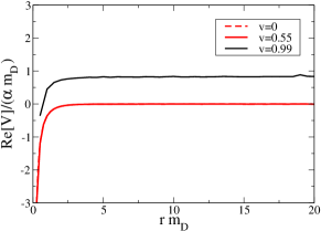
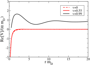
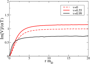
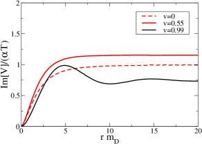
Figure 3: Real (upper panels) and imaginary (lower panels) parts of the potential between a quark and an antiquark moving with velocities $v=0$, $0.55$, $0.99$ with respect to the thermal bath. Right (left) panels correspond to the direction parallel (perpendicular) to the velocity of the thermal medium.

$v=0$

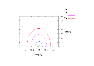
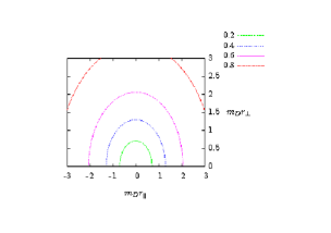
$v=0.5$

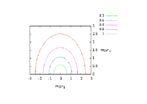
$v=0.9$

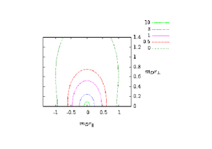
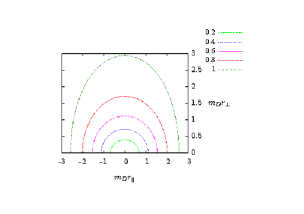
$v=0.99$

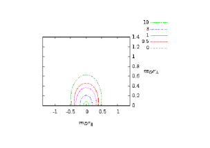
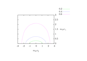
Figure 4: Contour lines of the two-body potential between a quark and antiquark moving with respect to the thermal bath with four different values of the velocity: $v=0,0.5,0.9,0.99$. The left panels correspond to the real part of the potential, while the right panels correspond to the imaginary part of the potential. The real part of the potential has been normalized to $\alpha m_{D}$, while the imaginary part of the potential has been normalized to $\alpha T$.

From the Fourier transform of the $\Delta_{11}$ propagator we have determined the real and imaginary parts of the potential in the HTL approximation. The potential is anisotropic, and in Fig. 3 we display the plots of the real (upper panels) and imaginary (lower panels) part of the potential for $v=0$, $v=0.55$, and $v=0.99$ respectively. We consider two directions: the first is along the direction of movement of the thermal bath (right panels) and the second one is along the direction orthogonal to the thermal bath (left panels). We plot only positive values of $r$ because the potential is symmetric for $r\to-r$. We normalize the real part of the potential to $\alpha m_{D}$, which describes the typical strength of the potential in the $v=0$ case. The imaginary part of the potential is normalized to $\alpha T$. With these normalizations the displayed shapes hold both for muonic hydrogen and for heavy quarkonium.

Regarding the real part, we observe that for $v\sim 0.55$ it is very similar (in fact, the curves overlap to a large extent) to the real part in the $v=0$ case, being Debye screened at a distance of order $m_{D}$ and not very asymmetric. For $v\sim 1$, however, although the real part of the potential remains Debye screened at roughly the same distance, it develops a rather large anisotropy. Indeed, an oscillation is observed in the direction of motion, which leads to the formation of a wake in the plasma.

Concerning the imaginary part of the potential for $v\sim 0.55$, it is not very asymmetric and remains very similar to the $v=0$ case. It monotonically increases and keeps the same pattern until $v\sim 0.9$. From that velocity on the imaginary part decreases and the anisotropy grows (see the $v=0.99$ curve). In the direction parallel to $\bf v$ one has that there is a mild increase with respect to the $v=0$ case for $r\simeq 4m_{D}$, and an oscillatory behavior at larger $r$ is also displayed. In the direction orthogonal to $\bf v$ there is an enhancement of the potential at short range and a decrease at large distances. Note that the imaginary part of the potential vanishes in the origin for any value of $v$ and in any direction.

In Fig. 4 we plot the contour lines for the real and imaginary parts of the two-body potentials between two heavy particles with opposite charges, for various values of the velocity. We focus on the short distance regime (the normalization for the real part is slightly different from the one in Fig. 3 because we have inverted the sign in order to match the normalization of Chu:1988wh ), because the distances relevant for dissociation are in the range $rm_{D}\lesssim 1$ Escobedo:2008sy . Various plots of the contour lines of the real part of the two-body potential were also shown in Chu:1988wh (see also Chakraborty:2006md ) and it can be seen that we obtained exactly the same results. The contour lines for the imaginary part of the two-body potential are reported for the first time here, and we observe that an important anisotropy exists even at short distances.

Let us next estimate the dissociation temperature in a way similar to refs. Escobedo:2008sy ; Escobedo:2010tu . If we assume that the typical momentum transfer $k$ is larger than the velocity dependent screening mass $m_{D}^{2}(v,\theta)\sim|\Pi_{R}(k,u)|$, we obtain that at $k\sim e^{2\over 3}T\sqrt{1-v^{2}}$ the real and the imaginary parts of the potential have the same size. For moderate velocities no qualitative change is expected with respect to the $v=0$ case. However, for $v$ close to $1$, $k$ becomes small and it is not guaranteed that the screening mass can be neglected in front of it. Indeed, we find that the screening mass remains finite for $v$ close to $1$ . This means that the typical $k$ for which the real and imaginary parts of the potential have the same size is smaller than the screening mass. Since a screened potential only supports bound states of a typical $k$ larger than $m_{D}(v,\theta)$, we conclude that at relativistic velocities, unlike the case of moderate velocities, the dissociation occurs due to screening (i.e. at the scale $T_{d}\sim m_{e}e$), as originally proposed by Matsui and Satz Matsui:1986dk , rather than due to Landau damping Laine:2006ns ; Escobedo:2008sy ; Brambilla:2008cx . This can also be qualitatively understood from our plots. For $v$ large and increasing, we see from Fig. 3 that the real part of the potential increases whereas the imaginary part decreases. Therefore, from some $v$ on, the real part of the potential dominates over the imaginary part and one can find the approximate wave functions of the system by solving a standard Schrödinger equation with a real potential. The decay width may be then calculated in perturbation theory by sandwiching the imaginary part of the potential between those wave functions. The wave functions of bound states go to a vanishing value at the distance where the real part of the potential becomes flat. From Fig. 4 it is also clear that the real part of the potential at short distances becomes steeper at increasing $v$. On the one hand this implies that no bound state exists from a certain velocity on. On the other hand it implies that when bound states still exist their wave functions are increasingly localized close to the origin. Since the imaginary part of the potential goes to zero at the origin, it follows that the decay width of such states is also going to zero at increasing $v$.

$v_{c}$ at which screening overtakes Landau damping as the dominant mechanism for dissociation, by equating $eT$ to $e^{2/3}T(1-v^{2})^{1/2}$ above. We obtain $v_{c}\sim\sqrt{1-ae^{2/3}}$, where $a$ is a numerical factor of order one . A quantitative study of all these issues may be carried out by numerically solving the Schrödinger equation with the full (complex) potential, for instance along the lines Burnier:2007qm ; Miao:2010tk ; Margotta:2011ta . This is however beyond the scope of this paper.

Regarding the real part of the potential, we find it interesting to compare the results reported in Fig. 3 with the recent results obtained for super Yang-Mills theory using AdS/CFT Liu:2006nn . For this theory it was stated that the potential could be approximated with a Yukawa potential and the dependence on the velocity encoded in a screening length that depends on $v$ and $\theta$ as follows:

$$m_{D}(v,\theta)=m_{D}(0,0)\frac{h(v,\theta)}{(1-v^{2})^{1/4}}\,,$$ (91)

where $h(v,\theta)$ is a function that is almost constant for any $v$ and $\theta$. The expression above does not give a good approximation of the potential in the HTL approximation. In particular the Debye screening for $v=0.99$ is strongly dependent on the angle $\theta$. If we try to fit the exponential behavior of the longitudinal and transverse directions, we find a screening length which is about a factor $2$ larger in the longitudinal direction with respect to the transverse direction. This can also be inferred from the fact that the scale of $m_{D}^{2}(v,\theta)$ must be given by $|\Pi_{R}(k,u)|$. We obtain in the case $v\to 1$

$$m_{D}(v,\theta)\sim\left\{\begin{array}[]{ll}m_{D}|\tan\theta|&{\rm if}\theta\nsim{\pi\over 2}\\ &\\ {m_{D}\over\sqrt{1-v^{2}}}&{\rm if}\theta\sim{\pi\over 2}\end{array}\right.$$ (92)

Be aware that the $\theta$ above is the angle between the velocity and the momentum transfer, whereas the $\theta$ in (91) is the angle between the velocity and the relative position. In any case, the expression (92) shows that at ultrarelativistic velocities a strong anisotropy for real space potential is expected, as confirmed by our figures and discussed above.

Regarding the oscillatory part of the potential one might wonder whether it is due to the weak coupling approximation. However, as shown in Jiang:2010zza for the potential produced by a single charge, in the HTL resummation approach the oscillations of the potential are larger than in the HTL approximation. Moreover, one would naively expect that with increasing coupling the wakes should be larger than in the weak coupling approximation.

VI Conclusions

The EFT theory for the description of bound states in a thermal medium has several interesting aspects. When the bound state moves with a moderate speed with respect to the medium the resulting EFT is quite similar to the one developed for the bound state at rest. We have taken into account the suitable modifications in Section III, for the hydrogen atom in the cases $T\ll 1/r$ and $T\sim 1/r$. However, when the speed is close to $1$, one has to consider two well separated scales, $T_{+}$ and $T_{-}$, defined in Eq. (8), and in the corresponding EFT one has collinear as well as soft degrees of freedom. The effective temperatures $T_{+}$ and $T_{-}$ can be in two different energy ranges and in Section IV we have considered two specific cases: the first one corresponds to $T_{+}\sim 1/r\gg T_{-}\gg E$ and the second one corresponds to $T_{+}\sim m_{e}\gg 1/r\gg T_{-}\gg E$. Note that in this case large logarithms of $T_{-}/T_{+}$ appear in the calculation. The factorized results displayed in Appendix B may be useful for a resummation of these large logarithms. It is reassuring that our results for moderate velocities are able to reproduce the ones obtained for the $v\sim 1$ case. For all the cases above we observe that the thermal decay width monotonically decreases with the velocity. This means that the faster the bound state moves across the thermal bath the more stable it becomes.

Finally, in Section V we have considered the case $T\gg 1/r$ allowing for light fermion pairs in the thermal bath. In atomic physics this state could be the muonic hydrogen in a thermal bath of electrons and positrons, while in heavy-ion collisions it may represent heavy quarkonia in the quark-gluon plasma at very high temperatures. We have determined how the imaginary and real component of the two-body potential are modified for nonvanishing velocities of the bound state with respect to the medium. Regarding the real part of the potential we have reproduced known results, and extended them to higher speeds. The imaginary part has been calculated for the first time. Its behavior is similar to the one determined for the thermal bath at rest for moderate velocities, but it tends to zero at velocities close to $1$. This implies that Landau damping Laine:2006ns ; Escobedo:2008sy ; Brambilla:2008cx is not the relevant mechanism for dissociation of bound states from a certain critical velocity $v_{c}$ on, which has been estimated in the previous section. Screening, as originally proposed by Matsui and Satz Matsui:1986dk , becomes then the relevant mechanism. Our results for the thermal decay width disagree with the qualitative estimate of ref. Dominguez:2008be , and with the more quantitative one of ref. Song:2007gm . We believe that the main reason for the discrepancy is due to the fact that the velocity dependence of the interaction is not properly taken into account in those works. Note that our results for the imaginary part depend crucially on the use of the correct non-equilibrium expression in Eq. (75), which leads to Eq. (90).

In the present paper we have paved the way for a more detailed study of the propagation of bound states in a thermal medium. We have assumed that the medium is a weakly coupled plasma, moving homogeneously and at a constant temperature, therefore our study needs a number of refinements to be realistically applied to HQ states in heavy-ion collisions. In that case, one should consider the expansion and cooling of the thermal medium, as well as possible anisotropies Burnier:2009yu ; Dumitru:2009fy ; Philipsen:2009wg ; Chandra:2010xg . In any case, we expect that the qualitative features we observe, namely that the decay width decreases with increasing velocity, and hence that Landau damping ceases to be the relevant mechanism for dissociation at a certain critical velocity, will remain true.

Appendix A Computation of $A$ and $B$ from section III

As a starting point one can use Eqs. (16) and (17) from Escobedo:2008sy , which for a bound state in a static thermal bath give

$$I_{ii}(q)=\frac{q}{2\pi^{2}}\left(\log\left(\frac{2\pi T}{|q|}\right)+\Re\Psi\left(\frac{i|q|}{2\pi T}\right)\right)\,.$$ (93)

This equation is obtained by a trivial angular integration because the system is symmetric under space rotations. When the bound state moves with respect to the thermal bath, the distribution function depends on the effective temperature defined in Eq. (5) and has a nontrivial dependence of the angle between $\bf k$ and $\bf v$. Now if we take into account the structure that was shown in Eq. (15) and define $x=\cos\theta$, we have that

$$\Im A(q)=\frac{q}{8\pi^{2}}\int_{-1}^{1}\,dx\left(\log\left(\frac{2\pi T\sqrt{1-v^{2}}}{|q|(1-vx)}\right)+\Re\Psi\left(\frac{i|q|(1-vx)}{2\pi T\sqrt{1-v^{2}}}\right)\right)\,,$$ (94)

and for the real part

$$\Re A(q)=\frac{1}{8\pi}\int_{-1}^{1}\,dx\frac{|q|}{e^{\frac{|q|(1-vx)}{T\sqrt{1-v^{2}}}}-1}\,.$$ (95)

Using Eq. (15) and the above equations we obtain that the imaginary and real part of the coefficient $B$ are respectively given by

$$\Im B(q)=\frac{q}{8\pi^{2}}\int_{-1}^{1}\,dxx^{2}\left(\log\left(\frac{2\pi T\sqrt{1-v^{2}}}{|q|(1-vx)}\right)+\Re\Psi\left(\frac{i|q|(1-vx)}{2\pi T\sqrt{1-v^{2}}}\right)\right)\,,$$ (96)

and

$$\Re B(q)=\frac{1}{8\pi}\int_{-1}^{1}\,dxx^{2}\frac{|q|}{e^{\frac{|q|(1-vx)}{2\pi T\sqrt{1-v^{2}}}}-1}\,.$$ (97)

As a cross-check, in the $v=0$ limit we find that the relation $B=\frac{A}{D-1}$ is fulfilled, and combining this with the identity

$$\delta_{ij}=\frac{3}{2}P^{s}_{ij}+\frac{1}{2}P^{p}_{ij}\,,$$ (98)

one recovers the results reported in Escobedo:2008sy .

Appendix B Computation of the contribution from ultrasoft photons in section IV

In this appendix we compute the matrix elements of $K_{ij}$ defined in Eq. (56) in the various integration regions identified in Section IV.

B.1 The $k_{+},k_{-}\sim T_{-}$ region

The quantities $a$ and $b$ defined in Eq. (58) can be computed from $K_{ij}$ as follows

$$a = \frac{2}{2D-4}K_{ii}+\frac{D-4}{2D-4}\frac{v^{i}v^{j}}{v^{2}}K_{ij}\,,$$ (99)

$$b = \frac{2}{2D-4}K_{ii}-\frac{D}{2D-4}\frac{v^{i}v^{i}}{v^{2}}K_{ij}\,,$$ (100)

and for $k_{+},k_{-}\sim T_{-}$ we find that

$$K_{ij}(q)=-2i\int\frac{\,d^{D}k}{(2\pi)^{D-1}}\frac{\delta(k_{+}k_{-}-k_{\perp}^{2})}{e^{\frac{|k_{-}|}{2T_{-}}}-1}\left(\delta_{ij}-\frac{k_{i}k_{j}}{k^{2}}\right)\left[\frac{1}{k_{+}+k_{-}-i\epsilon}+\frac{2q}{(k_{+}+k_{-}-i\epsilon)^{2}}+...\right]\,.$$ (101)

The first term in the square brackets vanishes by symmetry considerations and we find that

$$\Re K_{ii}(q) = 0\,,$$ (102)

$$\Im K_{ii}(q) = \frac{q}{2\pi^{2}}\left(\frac{1}{D-4}+\frac{1}{2}-\frac{\gamma}{2}+\frac{1}{2}\log\pi+\log\left(\frac{2T_{-}}{\mu}\right)\right)\,,$$ (103)

and

$$\Re\frac{v^{i}v^{j}}{v^{2}}K_{ij}(q) = 0\,,$$ (104)

$$\Im\frac{v^{i}v^{j}}{v^{2}}K_{ij}(q) = \frac{q}{6\pi^{2}}\left(\frac{1}{D-4}-\frac{\gamma}{2}+\frac{1}{2}\log\pi+\log\left(\frac{2T_{-}}{\mu}\right)\right)\,.$$ (105)

B.2 The case with $k_{+},k_{-}\sim q$

In this region we have that

$$K_{ij}(q)=i\int\frac{\,d^{D}k}{(2\pi)^{D-1}}\delta(k_{+}k_{-}-k_{\perp}^{2})\left(\frac{2T_{-}}{|k_{-}|}-\frac{1}{2}+...\right)\frac{1}{q-\frac{1}{2}(k_{+}+k_{-})+i\epsilon}\,,$$ (106)

and it is useful to calculate separately the imaginary part of the integrals with the first and the second terms in the brackets. The reason is that the computation of the first term in dimensional regularization is technically difficult, while the second one is quite straightforward.

We first compute the imaginary part of the term lineal in $T_{-}$ with a cut-off to separate the region $k_{+}\sim q$ from the region with $k_{-}\sim q(T_{-}/T_{+})$. Thus we consider a cut-off $\Lambda$ such that $q\gg\Lambda\gg q(T_{-}/T_{+})$ and we obtain

$$\Im K_{ii}(q)=2T_{-}\int_{0}^{\infty}\,dk_{+}\left[\frac{\log\left(\frac{\Lambda}{k_{+}+2q+i\epsilon}\right)}{k_{+}+2q+i\epsilon}+\frac{\log\left(\frac{\Lambda}{k_{+}+2q-i\epsilon}\right)}{k_{+}+2q-i\epsilon}-\frac{\log\left(\frac{\Lambda}{k_{+}-2q+i\epsilon}\right)}{k_{+}-2q+i\epsilon}-\frac{\log\left(\frac{\Lambda}{k_{+}-2q-i\epsilon}\right)}{k_{+}-2q-i\epsilon}\right]\,,$$ (107)

and

$$\Im\frac{v^{i}v^{j}}{v^{2}}K_{ij}(q)=0\,.$$ (108)

Then, the remaining terms are computed in dimensional regularization. Summing all the terms we obtain that

$$\Re K_{ii}(q) = \frac{T_{-}}{\pi}\left(\frac{1}{D-4}+\frac{1}{2}+\frac{\gamma}{2}-\frac{1}{2}\log\pi+\log\left(\frac{|q|}{\mu}\right)\right)-\frac{|q|}{4\pi}\,,$$ (109)

$$\Im K_{ii}(q) = -\frac{q}{2\pi^{2}}\left(\frac{1}{D-4}-\frac{1}{2}\log\pi+\log\left(\frac{|q|}{\mu}\right)-\frac{1}{2}+\frac{\gamma}{2}\right)$$ (110)

$$+ 2T_{-}\int_{0}^{\infty}\,dk_{+}\left[\frac{\log\left(\frac{\Lambda}{k_{+}+2q+i\epsilon}\right)}{k_{+}+2q+i\epsilon}+\frac{\log\left(\frac{\Lambda}{k_{+}+2q-i\epsilon}\right)}{k_{+}+2q-i\epsilon}-\frac{\log\left(\frac{\Lambda}{k_{+}-2q+i\epsilon}\right)}{k_{+}-2q+i\epsilon}-\frac{\log\left(\frac{\Lambda}{k_{+}-2q-i\epsilon}\right)}{k_{+}-2q-i\epsilon}\right]\,,$$

and

$$\frac{v^{i}v^{j}}{v^{2}}\Re K_{ij}(q) = \frac{T_{-}}{2\pi}-\frac{|q|}{6\pi}\,,$$ (111)

$$\frac{v^{i}v^{j}}{v^{2}}\Im K_{ij}(q) = -\frac{q}{6\pi^{2}}\left(\frac{1}{D-4}-\frac{5}{6}+\frac{\gamma}{2}-\frac{1}{2}\log\pi+\log\left(\frac{|q|}{\mu}\right)\right)\,.$$ (112)

B.3 The case with $k_{+}\sim q$, $k_{-}\sim q(T_{-}/T_{+})$

In this region we have that

$$K_{ij}(q)=2i\int\frac{\,d^{D}k}{(2\pi)^{D-1}}\frac{\delta(k_{+}k_{-}-k_{\perp}^{2})}{\left|\frac{k_{+}}{T_{+}}+\frac{k_{-}}{T_{-}}\right|}\left(\delta_{ij}-\frac{k_{i}k_{j}}{k^{2}}\right)\frac{1}{q-\frac{k_{+}}{2}+i\epsilon}\,.$$ (113)

For simplicity, we compute the imaginary part using a cut-off (as we did in the previous subsection) and the real part using dimensional regularization. We obtain that the real and imaginary parts of the trace of $K_{ij}$ are, respectively, given by

$$\Re K_{ii}(q) = -\frac{T_{-}}{\pi}\left(\frac{1}{D-4}+\frac{1}{2}+\frac{\gamma}{2}-\frac{1}{2}\log\pi+\log\left(\frac{|q|}{\mu}\right)+\frac{1}{2}\log\left(\frac{T_{-}}{T_{+}}\right)\right)\,,$$ (114)

$$\Im K_{ii}(q) = \frac{T_{-}}{2\pi^{2}}\int_{0}^{\infty}\,dk_{+}\left[\frac{P}{k_{+}+2q}-\frac{P}{k_{+}-2q}\right]\log\left(\frac{\Lambda T_{+}}{k_{+}T_{-}}\right)\,,$$ (115)

where $P$ stands for principal value. Moreover, we find that

$$\frac{v^{i}v^{j}}{v^{2}}\Re K_{ij}(q) = 0\,,$$ (116)

$$\frac{v^{i}v^{j}}{v^{2}}\Im K_{ij}(q) = 0\,.$$ (117)

Appendix C Interaction with collinear photons

In this appendix we give the detailed form of the part of the EFT’s Lagrangians that describes the interaction of electrons with collinear photons. General remarks about the matching are given in the corresponding subsections.

C.1 pNRQED Lagrangian for $T_{+}\sim 1/r$ and $1/r\gg T_{-}\gg E$

In this case the pNRQED Lagrangian has the form

$$\delta\mathcal{L}_{pNRQED} = c_{1}\frac{\psi^{\dagger}\psi}{m_{e}}\frac{\bar{n}^{\mu}F_{\mu i}}{(\bar{n}\partial)}\frac{\bar{n}^{\nu}F_{\nu i}}{(\bar{n}\partial)}+c_{2}\frac{\psi^{\dagger}\psi}{m_{e}}\frac{\bar{n}^{\mu}n^{\nu}F_{\mu\nu}}{(\bar{n}\partial)}\frac{\bar{n}^{\alpha}n^{\beta}F_{\alpha\beta}}{(\bar{n}\partial)}+c_{3}\frac{\psi^{\dagger}\psi}{m_{e}}\left[\frac{n^{\mu}F_{i\mu}}{(\bar{n}\partial)}\frac{\bar{n}^{\nu}F_{\nu i}}{(\bar{n}\partial)}+\frac{\bar{n}^{\mu}F_{i\mu}}{(\bar{n}\partial)}\frac{n^{\nu}F_{\nu i}}{(\bar{n}\partial)}\right]$$ (118)

$$+ c_{4}\frac{\psi^{\dagger}\psi}{m_{e}}\frac{n^{\mu}F_{i\mu}}{(\bar{n}\partial)}\frac{n^{\nu}F_{i\nu}}{(\bar{n}\partial)}+c_{5}\frac{\psi^{\dagger}\psi}{m_{e}}\left[\frac{\bar{n}^{\mu}n\partial F_{\mu i}}{(\bar{n}\partial)^{2}}\frac{\bar{n}^{\nu}F_{\nu i}}{(\bar{n}\partial)}+\frac{\bar{n}^{\mu}F_{\mu i}}{(\bar{n}\partial)}\frac{\bar{n}^{\nu}n\partial F_{\nu i}}{(\bar{n}\partial)^{2}}\right]$$

$$+ c_{6}\frac{\psi^{\dagger}\psi}{m_{e}}\left[\frac{\bar{n}^{\mu}n^{\nu}n\partial F_{\mu\nu}}{(\bar{n}\partial)^{2}}\frac{\bar{n}^{\alpha}n^{\beta}F_{\alpha\beta}}{(\bar{n}\partial)}+\frac{\bar{n}^{\mu}n^{\nu}F_{\mu\nu}}{(\bar{n}\partial)}\frac{\bar{n}^{\alpha}n^{\beta}n\partial F_{\alpha\beta}}{(\bar{n}\partial)^{2}}\right]$$

$$+ \frac{ic_{7}}{m_{e}^{2}}\left[\psi^{\dagger}\frac{\bar{n}^{\mu}n^{\nu}F_{\mu\nu}}{(\bar{n}\partial)}\frac{\bar{n}^{\alpha}n^{\beta}F_{\alpha\beta}}{(\bar{n}\partial)}D_{3}\psi-D_{3}\psi^{\dagger}\frac{\bar{n}^{\mu}n^{\nu}F_{\mu\nu}}{(\bar{n}\partial)}\frac{\bar{n}^{\alpha}n^{\beta}F_{\alpha\beta}}{(\bar{n}\partial)}\psi\right]$$

$$+ \frac{ic_{8}}{m_{e}^{2}}\left(\psi^{\dagger}\left[\frac{\bar{n}^{\mu}n^{\nu}F_{\mu\nu}}{(\bar{n}\partial)}\frac{\bar{n}^{\alpha}F_{\alpha i}}{(\bar{n}\partial)}+\frac{\bar{n}^{\mu}F_{\mu i}}{(\bar{n}\partial)}\frac{\bar{n}^{\alpha}n^{\beta}F_{\alpha\beta}}{(\bar{n}\partial)}\right]D_{i}\psi-D_{i}\psi^{\dagger}\left[\frac{\bar{n}^{\mu}n^{\nu}F_{\mu\nu}}{(\bar{n}\partial)}\frac{\bar{n}^{\alpha}F_{\alpha i}}{(\bar{n}\partial)}+\frac{\bar{n}^{\mu}F_{\mu i}}{(\bar{n}\partial)}\frac{\bar{n}^{\alpha}n^{\beta}F_{\alpha\beta}}{(\bar{n}\partial)}\right]\psi\right)$$

$$+ \frac{ic_{9}}{m_{e}^{2}}\left(D_{i}\psi^{\dagger}\left[\frac{\bar{n}^{\mu}F_{\mu j}}{(\bar{n}\partial)}\frac{\bar{n}^{\nu}\partial_{j}F_{\nu i}}{(\bar{n}\partial)^{2}}+\frac{\bar{n}^{\mu}\partial_{j}F_{\mu j}}{(\bar{n}\partial)^{2}}\frac{\bar{n}^{\nu}F_{\nu j}}{(\bar{n}\partial)}\right]\psi-\psi^{\dagger}\left[\frac{\bar{n}^{\mu}F_{\mu j}}{(\bar{n}\partial)}\frac{\bar{n}^{\nu}\partial_{j}F_{\nu i}}{(\bar{n}\partial)^{2}}+\frac{\bar{n}^{\mu}\partial_{j}F_{\mu j}}{(\bar{n}\partial)^{2}}\frac{\bar{n}^{\nu}F_{\nu j}}{(\bar{n}\partial)}\right]D_{i}\psi\right)$$

$$+ \frac{ic_{10}}{m_{e}^{2}}\left(D_{i}\psi^{\dagger}\left[\frac{n^{\mu}F_{i\mu}}{(\bar{n}\partial)}\frac{\bar{n}^{\nu}n^{\alpha}F_{\nu\alpha}}{(\bar{n}\partial)}+\frac{\bar{n}^{\mu}n^{\nu}F_{\mu\nu}}{(\bar{n}\partial)}\frac{n^{\alpha}F_{i\alpha}}{(\bar{n}\partial)}\right]\psi-\psi^{\dagger}\left[\frac{n^{\mu}F_{i\mu}}{(\bar{n}\partial)}\frac{\bar{n}^{\nu}n^{\alpha}F_{\nu\alpha}}{(\bar{n}\partial)}+\frac{\bar{n}^{\mu}n^{\nu}F_{\mu\nu}}{(\bar{n}\partial)}\frac{n^{\alpha}F_{i\alpha}}{(\bar{n}\partial)}\right]D_{i}\psi\right)\,.$$

The $\psi$ field is the field of the electron in pNRQED (we are using the form of pNRQED shown in Eq. (3) of Pineda:1997ie ), $D_{i}$ is the covariant derivative (containing ultrasoft photons only) that acts on the field of the electron and Latin indices stand always for transverse components.

The power counting for this Lagrangian works as follows. The leading order terms are the ones proportional to $c_{1}$ and $c_{2}$; note that the two terms in $\bar{n}^{\mu}F_{\mu i}$ are not of the same order of magnitude as $\bar{n}\partial A_{i}\gg\partial_{i}\bar{n}A$. Taking only the leading term of $F_{\mu\nu}$ in this two terms they have the form

$$c_{1}\frac{\psi^{\dagger}\psi A_{\perp}^{2}}{m_{e}}+c_{2}\frac{\psi^{\dagger}\psi(nA)^{2}}{m_{e}},$$ (119)

we consider that all the components of $A_{\mu}$ are of the same approximate size (this may not be true in some specific gauges). Starting from (119) each term that has an additional covariant derivative acting on an electron field is suppressed by an order $\alpha$, each transverse derivative acting on $A_{\mu}$ suppresses this term by an order $\sqrt{\frac{1-v}{1+v}}$ and each $(n\partial)$ acting on a $A_{\mu}$ field suppresses the term by an order $\frac{1-v}{1+v}$. If we consider that $\frac{1-v}{1+v}\gg\alpha\gg\left(\frac{1-v}{1+v}\right)^{3/2}$ the terms shown in Eq. (118) provide the complete list of operators at the order $m_{e}\alpha^{5}$. In practice only the two first terms contribute to our calculation. The Wilson coefficients are fixed by the matching calculation schematically shown in (52). We obtain

$$c_{1} = c_{2}=c_{4}=c_{9}=\frac{e^{2}}{2}\,,$$ (120)

$$c_{3} = c_{7}=c_{6}=c_{10}=-\frac{e^{2}}{2}\,,$$ (121)

$$c_{8} = c_{5}=\frac{e^{2}}{4}\,.$$ (122)

C.2 NRQED Lagrangian for $T_{+}\sim m_{e}$ and $1/r\gg T_{-}\gg E$

The full expression for the part of the NRQED Lagrangian that deals with the interaction of electrons with collinear photons is

$$\delta\mathcal{L}_{NRQED} = c_{1}\frac{\psi^{\dagger}\psi}{m_{e}}\frac{\bar{n}^{\mu}F_{\mu i}}{(\bar{n}\partial)}\frac{\bar{n}^{\nu}F_{\nu i}}{(\bar{n}\partial)}+c_{2}\frac{\psi^{\dagger}\psi}{m_{e}}\frac{\bar{n}^{\mu}n^{\nu}F_{\mu\nu}}{(\bar{n}\partial)}\frac{\bar{n}^{\alpha}n^{\beta}F_{\alpha\beta}}{(\bar{n}\partial)}+c_{3}\frac{\psi^{\dagger}\psi}{m_{e}}\left[\frac{n^{\mu}F_{i\mu}}{(\bar{n}\partial)}\frac{\bar{n}^{\nu}F_{\nu i}}{(\bar{n}\partial)}+\frac{\bar{n}^{\mu}F_{i\mu}}{(\bar{n}\partial)}\frac{n^{\nu}F_{\nu i}}{(\bar{n}\partial)}\right]$$ (123)

$$+ \frac{ic_{4}}{m_{e}^{2}}\left[\psi^{\dagger}\frac{\bar{n}^{\mu}n^{\nu}F_{\mu\nu}}{(\bar{n}\partial)}\frac{\bar{n}^{\alpha}n^{\beta}F_{\alpha\beta}}{(\bar{n}\partial)}D_{3}\psi-D_{3}\psi^{\dagger}\frac{\bar{n}^{\mu}n^{\nu}F_{\mu\nu}}{(\bar{n}\partial)}\frac{\bar{n}^{\alpha}n^{\beta}F_{\alpha\beta}}{(\bar{n}\partial)}\psi\right]$$

$$+ \frac{ic_{5}}{m_{e}^{2}}\left(\psi^{\dagger}\left[\frac{\bar{n}^{\mu}n^{\nu}F_{\mu\nu}}{(\bar{n}\partial)}\frac{\bar{n}^{\alpha}F_{\alpha i}}{(\bar{n}\partial)}+\frac{\bar{n}^{\mu}F_{\mu i}}{(\bar{n}\partial)}\frac{\bar{n}^{\alpha}n^{\beta}F_{\alpha\beta}}{(\bar{n}\partial)}\right]D_{i}\psi-D_{i}\psi^{\dagger}\left[\frac{\bar{n}^{\mu}n^{\nu}F_{\mu\nu}}{(\bar{n}\partial)}\frac{\bar{n}^{\alpha}F_{\alpha i}}{(\bar{n}\partial)}+\frac{\bar{n}^{\mu}F_{\mu i}}{(\bar{n}\partial)}\frac{\bar{n}^{\alpha}n^{\beta}F_{\alpha\beta}}{(\bar{n}\partial)}\right]\psi\right)$$

$$+ c_{6}\frac{\psi^{\dagger}\psi}{m_{e}}\frac{n^{\mu}F_{i\mu}}{(\bar{n}\partial)}\frac{n^{\nu}F_{i\nu}}{(\bar{n}\partial)}+c_{7}\frac{\psi^{\dagger}\psi}{m_{e}}\left[\frac{\bar{n}^{\mu}n\partial F_{\mu i}}{(\bar{n}\partial)^{2}}\frac{\bar{n}^{\nu}F_{\nu i}}{(\bar{n}\partial)}+\frac{\bar{n}^{\mu}F_{\mu i}}{(\bar{n}\partial)}\frac{\bar{n}^{\nu}n\partial F_{\nu i}}{(\bar{n}\partial)^{2}}\right]$$

$$+ c_{8}\frac{\psi^{\dagger}\psi}{m_{e}}\left[\frac{\bar{n}^{\mu}n^{\nu}n\partial F_{\mu\nu}}{(\bar{n}\partial)^{2}}\frac{\bar{n}^{\alpha}n^{\beta}F_{\alpha\beta}}{(\bar{n}\partial)}+\frac{\bar{n}^{\mu}n^{\nu}F_{\mu\nu}}{(\bar{n}\partial)}\frac{\bar{n}^{\alpha}n^{\beta}n\partial F_{\alpha\beta}}{(\bar{n}\partial)^{2}}\right]+\frac{ic_{9}}{m_{e}^{2}}\left(D_{i}\psi^{\dagger}\left[\frac{\bar{n}^{\mu}F_{\mu j}}{(\bar{n}\partial)}\frac{\bar{n}^{\nu}\partial_{j}F_{\nu i}}{(\bar{n}\partial)^{2}}+\frac{\bar{n}^{\mu}\partial_{j}F_{\mu j}}{(\bar{n}\partial)^{2}}\frac{\bar{n}^{\nu}F_{\nu j}}{(\bar{n}\partial)}\right]\psi\right.$$

$$- \left.\psi^{\dagger}\left[\frac{\bar{n}^{\mu}F_{\mu j}}{(\bar{n}\partial)}\frac{\bar{n}^{\nu}\partial_{j}F_{\nu i}}{(\bar{n}\partial)^{2}}+\frac{\bar{n}^{\mu}\partial_{j}F_{\mu j}}{(\bar{n}\partial)^{2}}\frac{\bar{n}^{\nu}F_{\nu j}}{(\bar{n}\partial)}\right]D_{i}\psi\right)+\frac{ic_{10}}{m_{e}^{2}}\left(D_{i}{\psi^{\dagger}}\left[\frac{n^{\mu}F_{i\mu}}{(\bar{n}\partial)}\frac{\bar{n}^{\nu}n^{\alpha}F_{\nu\alpha}}{(\bar{n}\partial)}+\frac{\bar{n}^{\mu}n^{\nu}F_{\mu\nu}}{(\bar{n}\partial)}\frac{n^{\alpha}F_{i\alpha}}{(\bar{n}\partial)}\right]\psi\right.$$

$$- \left.\psi^{\dagger}\left[\frac{n^{\mu}F_{i\mu}}{(\bar{n}\partial)}\frac{\bar{n}^{\nu}n^{\alpha}F_{\nu\alpha}}{(\bar{n}\partial)}+\frac{\bar{n}^{\mu}n^{\nu}F_{\mu\nu}}{(\bar{n}\partial)}\frac{n^{\alpha}F_{i\alpha}}{(\bar{n}\partial)}\right]D_{i}\psi\right)$$

$$+ \frac{1}{m_{e}^{3}}\left(D^{2}_{jj}\psi^{\dagger}\left[c_{11}\frac{\bar{n}^{\mu}F_{\mu i}}{(\bar{n}\partial)}\frac{\bar{n}^{\nu}F_{\nu i}}{(\bar{n}\partial)}+c_{12}\frac{\bar{n}^{\mu}n^{\nu}F_{\mu\nu}}{(\bar{n}\partial)}\frac{\bar{n}^{\alpha}n^{\beta}F_{\alpha\beta}}{(\bar{n}\partial)}\right]\psi\right.$$

$$+ \left.\psi^{\dagger}\left[c_{11}\frac{\bar{n}^{\mu}F_{\mu i}}{(\bar{n}\partial)}\frac{\bar{n}^{\nu}F_{\nu i}}{(\bar{n}\partial)}+c_{12}\frac{\bar{n}^{\mu}n^{\nu}F_{\mu\nu}}{(\bar{n}\partial)}\frac{\bar{n}^{\alpha}n^{\beta}F_{\alpha\beta}}{(\bar{n}\partial)}\right]D^{2}_{jj}\psi\right)$$

$$+ \frac{1}{m_{e}^{3}}D_{j}\psi^{\dagger}\left[c_{13}\frac{\bar{n}^{\mu}F_{\mu i}}{(\bar{n}\partial)}\frac{\bar{n}^{\nu}F_{\nu i}}{(\bar{n}\partial)}+c_{14}\frac{\bar{n}^{\mu}n^{\nu}F_{\mu\nu}}{(\bar{n}\partial)}\frac{\bar{n}^{\alpha}n^{\beta}F_{\alpha\beta}}{(\bar{n}\partial)}\right]D_{j}\psi$$

$$+ \frac{c_{15}}{m_{e}^{3}}\left(D^{2}_{33}\psi^{\dagger}\frac{\bar{n}^{\mu}n^{\nu}F_{\mu\nu}}{(\bar{n}\partial)}\frac{\bar{n}^{\alpha}n^{\beta}F_{\alpha\beta}}{(\bar{n}\partial)}\psi+\psi^{\dagger}\frac{\bar{n}^{\mu}n^{\nu}F_{\mu\nu}}{(\bar{n}\partial)}\frac{\bar{n}^{\alpha}n^{\beta}F_{\alpha\beta}}{(\bar{n}\partial)}D^{2}_{33}\psi\right)$$

$$+ \frac{c_{16}}{m_{e}^{3}}D_{3}\psi^{\dagger}\frac{\bar{n}^{\mu}n^{\nu}F_{\mu\nu}}{(\bar{n}\partial)}\frac{\bar{n}^{\alpha}n^{\beta}F_{\alpha\beta}}{(\bar{n}\partial)}D_{3}\psi+\frac{c_{17}}{m_{e}^{3}}\left(D^{2}_{3i}\psi^{\dagger}\left[\frac{\bar{n}^{\mu}n^{\nu}F_{\mu\nu}}{(\bar{n}\partial)}\frac{\bar{n}^{\alpha}F_{\alpha i}}{(\bar{n}\partial)}+\frac{\bar{n}^{\mu}F_{\mu i}}{(\bar{n}\partial)}\frac{\bar{n}^{\nu}n^{\alpha}F_{\nu\alpha}}{(\bar{n}\partial)}\right]\psi\right.$$

$$- \left.D_{3}\psi^{\dagger}\left[\frac{\bar{n}^{\mu}n^{\nu}F_{\mu\nu}}{(\bar{n}\partial)}\frac{\bar{n}^{\alpha}F_{\alpha i}}{(\bar{n}\partial)}+\frac{\bar{n}^{\mu}F_{\mu i}}{(\bar{n}\partial)}\frac{\bar{n}^{\nu}n^{\alpha}F_{\nu\alpha}}{(\bar{n}\partial)}\right]D_{i}\psi-D_{i}\psi^{\dagger}\left[\frac{\bar{n}^{\mu}n^{\nu}F_{\mu\nu}}{(\bar{n}\partial)}\frac{\bar{n}^{\alpha}F_{\alpha i}}{(\bar{n}\partial)}+\frac{\bar{n}^{\mu}F_{\mu i}}{(\bar{n}\partial)}\frac{\bar{n}^{\nu}n^{\alpha}F_{\nu\alpha}}{(\bar{n}\partial)}\right]D_{3}\psi\right.$$

$$+ \left.\psi^{\dagger}\left[\frac{\bar{n}^{\mu}n^{\nu}F_{\mu\nu}}{(\bar{n}\partial)}\frac{\bar{n}^{\alpha}F_{\alpha i}}{(\bar{n}\partial)}+\frac{\bar{n}^{\mu}F_{\mu i}}{(\bar{n}\partial)}\frac{\bar{n}^{\nu}n^{\alpha}F_{\nu\alpha}}{(\bar{n}\partial)}\right]D^{2}_{3i}\psi\right)\,.$$

The power counting for this expression is the same as in Eq. (118). However, we are considering now higher velocities, and hence the relative size of $\frac{1-v}{1+v}$ and $\alpha$ differs from the previous case. For $\frac{1-v}{1+v}\gg\alpha^{2}\gg\left(\frac{1-v}{1+v}\right)^{3/2}$ we have listed above all the operators up to the order of $m_{e}\alpha^{5}$. In practice, only the operators proportional to $c_{1}$, $c_{2}$, $c_{11}$ and $c_{13}$ contribute to our calculation. The Wilson coefficients are fixed by the matching calculation sketched in (69). We obtain

$$c_{1} = c_{2}=c_{6}=c_{9}=\frac{e^{2}}{2}\,,$$ (124)

$$c_{3} = c_{4}=c_{10}=c_{8}=-\frac{e^{2}}{2}\,,$$ (125)

$$c_{5} = c_{7}=c_{16}=\frac{e^{2}}{4}\,,$$ (126)

$$c_{11} = c_{12}=\frac{3e^{2}}{16}\,,$$ (127)

$$c_{13} = c_{14}=c_{17}=\frac{e^{2}}{8}\,,$$ (128)

$$c_{15} = -\frac{3e^{2}}{8}\,.$$ (129)

References

- (1) P. M. Echenique, F. Flores and R. H. Ritchie, Solid State Phys. 43, 229 (1990).
- (2) T. Matsui and H. Satz, Phys. Lett. B 178, 416 (1986).
- (3) C. Lourenco, Nucl. Phys. A 783, 451 (2007) [arXiv:nucl-ex/0612014].
- (4) M. C. Chu and T. Matsui, Phys. Rev. D 39, 1892 (1989).
- (5) N. Armesto et al., J. Phys. G 35, 054001 (2008) [arXiv:0711.0974 [hep-ph]].
- (6) M. G. Mustafa, M. H. Thoma and P. Chakraborty, Phys. Rev. C 71, 017901 (2005) [arXiv:hep-ph/0403279].
- (7) J. Ruppert and B. Muller, Phys. Lett. B 618, 123 (2005) [arXiv:hep-ph/0503158].
- (8) P. Chakraborty, M. G. Mustafa and M. H. Thoma, Phys. Rev. D 74, 094002 (2006) [arXiv:hep-ph/0606316].
- (9) P. Chakraborty, M. G. Mustafa, R. Ray and M. H. Thoma, J. Phys. G 34, 2141 (2007) [arXiv:0705.1447 [hep-ph]].
- (10) B. F. Jiang and J. R. Li, Nucl. Phys. A 832, 100 (2010).
- (11) T. C. Awes [PHENIX Collaboration], J. Phys. G 35, 104007 (2008) [arXiv:0805.1636 [nucl-ex]].
- (12) H. van Hees, M. Mannarelli, V. Greco and R. Rapp, Phys. Rev. Lett. 100, 192301 (2008) [arXiv:0709.2884 [hep-ph]].
- (13) M. C. Abreu et al. [NA50 Collaboration], Phys. Lett. B 410, 337 (1997).
- (14) M. A. Escobedo and J. Soto, Phys. Rev. A 78, 032520 (2008) [arXiv:0804.0691 [hep-ph]].
- (15) N. Brambilla, J. Ghiglieri, A. Vairo and P. Petreczky, Phys. Rev. D 78, 014017 (2008) [arXiv:0804.0993 [hep-ph]].
- (16) N. Brambilla, M. A. Escobedo, J. Ghiglieri, J. Soto and A. Vairo, JHEP 1009, 038 (2010) [arXiv:1007.4156 [hep-ph]].
- (17) M. Laine, O. Philipsen, P. Romatschke and M. Tassler, JHEP 0703, 054 (2007) [arXiv:hep-ph/0611300].
- (18) C. W. Bauer, S. Fleming and M. E. Luke, Phys. Rev. D 63, 014006 (2000) [arXiv:hep-ph/0005275].
- (19) W. E. Caswell and G. P. Lepage, Phys. Lett. B 167, 437 (1986).
- (20) A. Pineda and J. Soto, Nucl. Phys. Proc. Suppl. 64, 428 (1998) [arXiv:hep-ph/9707481].
- (21) A. Pineda and J. Soto, Phys. Lett. B 420, 391 (1998) [arXiv:hep-ph/9711292].
- (22) A. Pineda and J. Soto, Phys. Rev. D 59, 016005 (1999) [arXiv:hep-ph/9805424].
- (23) M. A. Escobedo and J. Soto, Phys. Rev. A 82, 042506 (2010) [arXiv:1008.0254 [hep-ph]].
- (24) H. A. Weldon, Phys. Rev. D 26, 1394 (1982).
- (25) M. E. Carrington, D. f. Hou and M. H. Thoma, Eur. Phys. J. C 7, 347 (1999) [arXiv:hep-ph/9708363].
- (26) J. J. Sakurai, Moderm Quantum Mechanics, Addison-Wesley Company (1994).
- (27) M.I. Eides, H. Grotch, V.A. Shelyuto, Phys. Rep. 342, 63 (2001).
- (28) Kottmann et al., Hyperfine Interact., 138, 55 (2001); R. Pohl et al., Nature 466, 213 (2010).
- (29) F.C. Frank, Nature 160, 525 (1947); J.D. Jackson, Phys. Rev. 106, 330 (1957).
- (30) Riken collaboration, Muon catalyzed fusion for energy production; see http://www.rikenresearch.riken.jp/eng/frontline/5976
- (31) Star collaboration, Muon catalyzed fusion; see http://www.starscientific.com.au/
- (32) M. Chernicoff, J. A. Garcia and A. Guijosa, JHEP 0609 (2006) 068 [arXiv:hep-th/0607089].
- (33) K. Peeters, J. Sonnenschein and M. Zamaklar, Phys. Rev. D 74, 106008 (2006) [arXiv:hep-th/0606195].
- (34) H. Liu, K. Rajagopal and U. A. Wiedemann, Phys. Rev. Lett. 98, 182301 (2007) [arXiv:hep-ph/0607062].
- (35) P. M. Chesler and L. G. Yaffe, Phys. Rev. Lett. 99, 152001 (2007) [arXiv:0706.0368 [hep-th]].
- (36) Y. Burnier, M. Laine and M. Vepsalainen, JHEP 0801, 043 (2008) [arXiv:0711.1743 []].
- (37) C. Miao, A. Mocsy and P. Petreczky, arXiv:1012.4433 [hep-ph].
- (38) M. Margotta, K. McCarty, C. McGahan, M. Strickland and D. Yager-Elorriaga, arXiv:1101.4651 [hep-ph].
- (39) F. Dominguez and B. Wu, Nucl. Phys. A 818, 246 (2009) [arXiv:0811.1058 [hep-ph]].
- (40) T. Song, Y. Park, S. H. Lee and C. Y. Wong, Phys. Lett. B 659, 621 (2008) [arXiv:0709.0794 [hep-ph]].
- (41) Y. Burnier, M. Laine and M. Vepsalainen, Phys. Lett. B 678, 86 (2009) [arXiv:0903.3467 [hep-ph]].
- (42) A. Dumitru, Y. Guo and M. Strickland, Phys. Rev. D 79, 114003 (2009) [arXiv:0903.4703 [hep-ph]].
- (43) O. Philipsen and M. Tassler, arXiv:0908.1746 [hep-ph].
- (44) V. Chandra and V. Ravishankar, Nucl. Phys. A 848, 330 (2010) [arXiv:1006.3995 [nucl-th]].