∎

Transformation elastodynamics and active exterior acoustic cloaking

Coordinate transformations can be used to manipulate fields in a variety of ways for the Maxwell and Helmholtz equations. In Sect. 1 we focus on transformation elastodynamics. The idea is to manipulate waves in an elastic medium by designing appropriate transformations of the coordinates and the displacements. As opposed to the Maxwell and Helmholtz equations, the elastodynamic equations are not invariant under these transformations. Here we recall the transformed elastodynamic equations, and then move to the effect of space transformations on a mass-spring network model. In order to realize the transformed networks we introduce “torque springs”, which are springs with a force proportional to the displacement in a direction other than the direction dictated by the spring terminals. We discuss some possible homogenizations of transformed networks that could have applications to manipulating waves in an elastic medium for e.g. cloaking.

Then we look at an approach to cloaking which is based on cancelling the incident field using active devices (rather than passive composite materials) which are exterior to the cloaked region. Exterior means that the cloaked region is not completely surrounded by the cloak, as is the case in most transformation based methods. We present here active exterior cloaking methods for both the Laplace equation in dimension two (Sect. 2) and the Helmholtz equation in dimension three (Sect. 3).

The cloaking method for the Laplace equation we present in Sect. 2 applies also to the quasi-static (low frequency) regime and was in part presented in Guevara Vasquez et al (2011c, 2009a). We first reformulate the problem of designing an active cloaking device as the classic problem of approximating analytic functions with polynomials. This theoretical approach shows that it is possible to cloak an object from an incident field with one single exterior device. Then we give an explicit solution to the problem in terms of a polynomial and determine its convergence region as the degree of the polynomial increases. This convergence region limits the size of the cloaked region, and for the new solution we propose here it allows one to cloak larger objects at a fixed distance from the device compared to the explicit polynomial solution given in Guevara Vasquez et al (2011c, 2009a). We also discuss how our approach can be modified to simultaneously hide an object and give the illusion of another object, in the same spirit as illusion optics Lai et al (2009).

Next in Sect. 3 we consider the Helmholtz equation and use the same techniques as in Guevara Vasquez et al (2011b) to show that in dimension three it is possible to cloak an object using four devices and yet leaving the object connected with the exterior. Our method is based on Green’s formula, which ensures that an analytic field can be reproduced inside a volume by a carefully chosen single and double layer potential at the surface of the volume. Then we use addition theorems for spherical outgoing waves to concentrate the single and double layer potential at a few multipolar sources (cloaking devices) located outside the cloaked region. We determine the convergence region of the device’s field and include an explicit geometric construction of a cloak with four devices.

The three sections of this chapter can be read essentially independently of each other.

1 Transformation elastodynamics

Transformation based cloaking was first discovered by Greenleaf, Lassas and Uhlmann Greenleaf et al (2003a, b) in the context of the conductivity equations. Independently, Leonhardt realized that transformation based cloaking applies to geometric optics Leonhardt (2006) and Pendry, Schurig and Smith Pendry et al (2006) realized that transformation based cloaking applies to Maxwell’s equations at fixed frequency, and this led to an explosion of interest in the field. It was found that transformation based cloaking also applies to acoustics Cummer and Schurig (2007); Chen and Chan (2007); Greenleaf et al (2007), which is governed by the Helmholtz equation, provided one permits anisotropic density Schoenberg and Sen (1983). These developments, reviewed in Alú and Engheta (2008); Greenleaf et al (2009); Cai and Shalaev (2010); Chen and Chan (2010) rely on the invariance of the conductivity equations, Maxwell’s equations, and the Helmholtz equation under coordinate transformations, and have been substantiated by rigorous proofs Greenleaf et al (2007); Kohn et al (2008, 2010). The invariance of Maxwell’s equations under coordinate transformations has led to other envisaged applications such as field concentrators Rahm et al (2008), field rotators Chen et al (2009), lenses Schurig (2008), superscatterers Yang et al (2008) (see also Nicorovici et al (1994)) and the name “transformation optics” is now used to describe this research: see, for example, the special issue in the New Journal of Physics Leonhardt and Smith (2008) devoted to cloaking and transformation optics. The perfect lens of Pendry Pendry (2000) can be viewed as the result of using a transformation which unfolds space Leonhardt and Philbin (2006) and associated with such folding transformations is cloaking due to anomalous resonance Milton and Nicorovici (2006); Nicorovici et al (2007); Milton et al (2008).

A largely open question is how to construct metamaterials with the required combination of anisotropic electrical permittivity $\mbox{\boldmath${\varepsilon}$}({\bf x})$ and anisotopic magnetic permeability $\mbox{\boldmath${\mu}$}({\bf x})$ needed in transformation optics designs, frequently with $\mbox{\boldmath${\varepsilon}$}({\bf x})=\mbox{\boldmath${\mu}$}({\bf x})$. Only recently was it shown Milton (2010), building upon work of Bouchitté and Schweizer Bouchitté and Schweizer (2010), that any combination of real tensors $(\mbox{\boldmath${\varepsilon}$},\mbox{\boldmath${\mu}$})$ is approximately realizable, at least in theory.

Curiously, the usual elastodynamic equations do not generally keep their form under coordinate transformations. Either new terms enter the equations Milton et al (2006), so they take the form of equations Willis introduced Willis (1981) to describe the ensemble averaged elastodynamic behavior of composite materials (which are the analog of the bianisotropic equations of electromagnetism Serdikukov et al (2001)), or the elasticity tensor field does not retain its minor symmetries Brun et al (2009). Nevertheless, as shown in Milton (2007) and as is explored further here, there is some hope that metamaterials can be constructed with a response corresponding approximately with that required by the new equations.

1.1 Continuous transformation elastodynamics

By extending the analysis of Milton et al (2006), let us show that the equation of elastodynamics

$$-\nabla\cdot({\bf C}({\bf x})\nabla{\bf u})=\omega^{2}\rho({\bf x}){\bf u}$$ (1)

changes under the transformation

$${\bf x}^{\prime}={\bf x}^{\prime}({\bf x}),\quad{\bf u}^{\prime}({\bf x}^{\prime}({\bf x}))=({\bf B}^{T}({\bf x}))^{-1}{\bf u}({\bf x})$$ (2)

to the equation

$$-\nabla^{\prime}\cdot({\bf C}^{\prime}({\bf x}^{\prime})\nabla^{\prime}{\bf u}^{\prime}+{\bf S}^{\prime}({\bf x}^{\prime}){\bf u}^{\prime})+{\bf D}^{\prime}({\bf x}^{\prime})\nabla^{\prime}{\bf u}^{\prime}-\omega^{2}(\mbox{\boldmath${\rho}$}^{\prime}({\bf x}^{\prime}){\bf u}^{\prime})=0$$ (3)

where the tensors ${\bf C}^{\prime}$, ${\bf S}^{\prime}$, ${\bf D}^{\prime}$, $\mbox{\boldmath${\rho}$}^{\prime}$ are given in terms of the functions ${\bf x}^{\prime}$, ${\bf B}$ and their derivatives. Here the transformation of the displacement is governed by ${\bf B}({\bf x})$ which can be chosen to be any invertible matrix valued function. (The inverse and transpose in $({\bf B}^{T}({\bf x}))^{-1}$ have been introduced to simplify subsequent formulae.)

Indeed let us first note that

$$\nabla{\bf u} = \frac{\partial u_{j}}{\partial x_{i}}=\frac{\partial(u^{\prime}_{p}B_{pj})}{\partial x_{i}}=\frac{\partial x_{m}^{\prime}}{\partial x_{i}}\frac{\partial u^{\prime}_{p}}{\partial x^{\prime}_{m}}B_{pj}+\frac{\partial B_{pj}}{\partial x_{i}}u^{\prime}_{p}$$ (4)

$$= {\bf A}^{T}(\nabla^{\prime}{\bf u}^{\prime}){\bf B}+{\bf G}^{\prime}{\bf u}^{\prime}$$

in which ${\bf A}$ and ${\bf G}$ are the tensors with elements

$$A_{mi}=\frac{\partial x_{m}^{\prime}}{\partial x_{i}},\quad G_{ijp}=\frac{\partial B_{pj}}{\partial x_{i}}.$$ (5)

Now (1) implies that for all smooth vector-valued test functions ${\bf v}({\bf x})$ with compact support in a domain $\Omega$,

$$0 =\int_{\Omega}[-\nabla\cdot({\bf C}({\bf x})\nabla{\bf u})-\omega^{2}\rho({\bf x}){\bf u}]\cdot{\bf v}~{}\mathrm{d}{\bf x}$$

$$=\int_{\Omega}[{\bf C}({\bf x})\nabla{\bf u}:\nabla{\bf v}-\omega^{2}\rho({\bf x}){\bf u}\cdot{\bf v}]~{}\mathrm{d}{\bf x}$$

$$=\int_{\Omega^{\prime}}[{\bf C}({\bf x})({\bf A}^{T}(\nabla^{\prime}{\bf u}^{\prime}){\bf B}+{\bf G}{\bf u}^{\prime}):({\bf A}^{T}(\nabla^{\prime}{\bf v}^{\prime}){\bf B}+{\bf G}{\bf v}^{\prime})-\omega^{2}\rho({\bf x})({\bf B}^{T}{\bf u}^{\prime})\cdot({\bf B}^{T}{\bf v}^{\prime})]a^{-1}~{}\mathrm{d}{\bf x}^{\prime}$$

$$=\int_{\Omega^{\prime}}[{\bf C}^{\prime}({\bf x}^{\prime})\nabla^{\prime}{\bf u}^{\prime}:\nabla^{\prime}{\bf v}^{\prime}+{\bf S}^{\prime}({\bf x}^{\prime}){\bf u}^{\prime}:\nabla^{\prime}{\bf v}^{\prime}+({\bf D}^{\prime}({\bf x}^{\prime})\nabla^{\prime}{\bf u}^{\prime})\cdot{\bf v}^{\prime}-\omega^{2}(\mbox{\boldmath${\rho}$}^{\prime}({\bf x}^{\prime}){\bf u}^{\prime})\cdot{\bf v}^{\prime}]~{}\mathrm{d}{\bf x}^{\prime}$$

$$=\int_{\Omega^{\prime}}[-\nabla^{\prime}\cdot({\bf C}^{\prime}({\bf x}^{\prime})\nabla^{\prime}{\bf u}^{\prime}+{\bf S}^{\prime}({\bf x}^{\prime}){\bf u}^{\prime})+{\bf D}^{\prime}({\bf x}^{\prime})\nabla^{\prime}{\bf u}^{\prime}-\omega^{2}(\mbox{\boldmath${\rho}$}^{\prime}({\bf x}^{\prime}){\bf u}^{\prime})]\cdot{\bf v}^{\prime}~{}\mathrm{d}{\bf x}^{\prime}$$

in which the test function ${\bf v}({\bf x})$ has been transformed, similarly to ${\bf u}({\bf x})$, to

$${\bf v}^{\prime}({\bf x}^{\prime}({\bf x}))=({\bf B}^{T}({\bf x}))^{-1}{\bf v}({\bf x}),$$ (7)

and $a({\bf x}^{\prime}({\bf x}))=\det{\bf A}({\bf x})$ while ${\bf C}^{\prime}({\bf x}^{\prime})$, ${\bf S}^{\prime}({\bf x}^{\prime})$, ${\bf D}^{\prime}({\bf x}^{\prime})$ and $\mbox{\boldmath${\rho}$}^{\prime}({\bf x}^{\prime})$ are the tensors with elements

$$C^{\prime}_{ijk\ell} = a^{-1}A_{ip}B_{jq}A_{kr}B_{\ell s}C_{pqrs},$$

$$S^{\prime}_{ijk} = a^{-1}A_{ip}B_{jq}G_{rsk}C_{pqrs}=a^{-1}A_{ip}B_{jq}\frac{\partial B_{ks}}{\partial x^{\prime}_{r}}C_{pqrs},$$

$$D^{\prime}_{kij} = a^{-1}G_{pqk}A_{ir}B_{js}C_{pqrs}=S^{\prime}_{ijk},$$

$$\rho^{\prime}_{ij} = a^{-1}B_{ik}B_{jk}\rho-a^{-1}\omega^{-2}G_{pqi}G_{rsj}C_{pqrs}$$ (8)

$$= a^{-1}B_{ik}B_{jk}\rho-a^{-1}\omega^{-2}\frac{\partial B_{iq}}{\partial x^{\prime}_{p}}\frac{\partial B_{js}}{\partial x^{\prime}_{r}}C_{pqrs}.$$

From (LABEL:a.5) we see directly that (1) transforms to (3).

Remark 1

The transformed elastodynamic equation (3) can be written in the equivalent form of Willis-type equations Willis (1981)

$$\nabla^{\prime}\cdot\mbox{\boldmath${\sigma}$}^{\prime} = -i\omega{\bf p}^{\prime},$$

$$\quad\mbox{\boldmath${\sigma}$}^{\prime} = {\bf C}^{\prime}({\bf x}^{\prime})\nabla^{\prime}{\bf u}^{\prime}+(i/\omega){\bf S}^{\prime}({\bf x}^{\prime})(-i\omega{\bf u}^{\prime}),$$

$${\bf p}^{\prime} = \mbox{\boldmath${\rho}$}^{\prime}({\bf x}^{\prime})(-i\omega{\bf u}^{\prime})+(i/\omega){\bf D}^{\prime}({\bf x}^{\prime})\nabla{\bf u}^{\prime},$$ (9)

in which the stress $\mbox{\boldmath${\sigma}$}^{\prime}$, which is not necessarily symmetric, depends not only upon the dispacement gradient $\nabla^{\prime}{\bf u}^{\prime}$ but also upon the velocity $-i\omega{\bf u}^{\prime}$, and the momentum ${\bf p}^{\prime}$ depends not only upon the velocity $-i\omega{\bf u}^{\prime}$, but also on the displacement gradient $\nabla^{\prime}{\bf u}^{\prime}$.

Remark 2

If we desire the transformed elasticity tensor ${\bf C}^{\prime}({\bf x}^{\prime})$ to have all the usual symmetries of elasticity tensors, namely that

$$C^{\prime}_{ijk\ell}=C^{\prime}_{jik\ell}=C^{\prime}_{k\ell ij},$$ (10)

then we need to restrict the transformations to those with ${\bf B}={\bf A}$. This was the case analyzed by Milton, Briane and Willis Milton et al (2006).

Remark 3

In the particular case where ${\bf B}={\bf I}$ the transformation (8) reduces to

$$C^{\prime}_{ijk\ell} = a^{-1}A_{ip}A_{kr}C_{pjr\ell},\quad{\bf S}^{\prime}={\bf D}^{\prime}=0,\quad\mbox{\boldmath${\rho}$}^{\prime}=a^{-1}\rho{\bf I},$$ (11)

corresponding to normal elastodynamics, with an isotropic density matrix $\mbox{\boldmath${\rho}$}^{\prime}$, but with an elasticity tensor ${\bf C}^{\prime}$ only satisfying the major symmetry $C^{\prime}_{ijk\ell}=C^{\prime}_{k\ell ij}$. This was the case analysed by Brun, Guenneau and Movchan Brun et al (2009) in a particular two-dimensional example.

Having derived the rules of transformation elasticity, one can then apply the same variety of transformations as used in transformation optics, including cloaking and folding transformations. The point is that a wave propagating classically in the classical medium can have a strange behavior in the new abstract coordinate system ${\bf x}^{\prime}$. If we are able to design a real medium following a system of equations equivalent to the transformed system, then we are able to force a strange behavior for waves in real physical space.

1.2 Discrete transformation elastodynamics

There is a discrete version of the transformation (11). Suppose we have a network of springs, possibly a lattice infinite in extent, with a countable number of nodes at positions ${\bf x}_{1},{\bf x}_{2},{\bf x}_{3},\ldots,{\bf x}_{n}\ldots$, at which there are masses $M_{1},M_{2},M_{3},\ldots,M_{n}\ldots$, and at which the displacements are ${\bf u}_{1},{\bf u}_{2},{\bf u}_{3},\ldots,{\bf u}_{n}\ldots$. Let $k_{ij}$ denote the spring constant of the spring connecting node $i$ to node $j$. There is no loss of generality in assuming that all pairs of nodes are joined by a spring, taking $k_{ij}=0$ if there is no real spring joining node $i$ and $j$. Let ${\bf F}_{i,j}$ denote the force which the spring joining nodes $i$ and $j$ exerts on node $i$. Hooke’s law implies

$${\bf F}_{i,j}=-{\bf F}_{j,i}=k_{i,j}{\bf n}_{i,j}[{\bf n}_{i,j}\cdot({\bf u}_{j}-{\bf u}_{i})],$$ (12)

where

$${\bf n}_{i,j}=\frac{{\bf x}_{j}-{\bf x}_{i}}{|{\bf x}_{j}-{\bf x}_{i}|},$$ (13)

is the unit vector in the direction of ${\bf x}_{j}-{\bf x}_{i}$. In the absence of any forces acting on the nodes, apart from inertial forces, Newton’s second law implies

$$\sum_{j}{\bf F}_{i,j}=-M_{i}\omega^{2}{\bf u}_{i}.$$ (14)

Now let us consider a transformation ${\bf x}^{\prime}={\bf x}^{\prime}({\bf x})$ with an associated inverse transformation ${\bf x}={\bf x}({\bf x}^{\prime})$. Under this transformation the position of the nodes transform to ${\bf x}^{\prime}_{1},{\bf x}^{\prime}_{2},{\bf x}^{\prime}_{3},\ldots,{\bf x}^{\prime}_{n}\ldots$, where ${\bf x}^{\prime}_{i}={\bf x}^{\prime}({\bf x}_{i})$. We focus, for simplicity, on the case corresponding to ${\bf B}={\bf I}$ where the forces, masses and displacements transform according to

$${\bf F}^{\prime}_{i,j}={\bf F}_{i,j},\quad M^{\prime}_{i}=M_{i},\quad{\bf u}^{\prime}_{i}={\bf u}_{i}.$$ (15)

After the transformation, Newton’s second law clearly keeps its form,

$$\sum_{j}{\bf F}^{\prime}_{i,j}=-M^{\prime}_{i}\omega^{2}{\bf u}^{\prime}_{i},$$ (16)

while (12) transforms to

$${\bf F}^{\prime}_{i,j}=-{\bf F}^{\prime}_{j,i}=k^{\prime}_{i,j}{\bf v}^{\prime}_{i,j}[{\bf v}^{\prime}_{i,j}\cdot({\bf u}^{\prime}_{j}-{\bf u}^{\prime}_{i})]$$ (17)

where

$$k^{\prime}_{i,j}=k_{i,j},\quad{\bf v}^{\prime}_{i,j}=\frac{{\bf x}({\bf x}^{\prime}_{j})-{\bf x}({\bf x}^{\prime}_{i})}{|{\bf x}({\bf x}^{\prime}_{j})-{\bf x}({\bf x}^{\prime}_{i})|}$$ (18)

Hence in the new coordinates ${\bf x}^{\prime}_{i}$ the system is governed by equations similar to the classical system of equations for a network of masses joined by springs, but the response of the springs does not anymore correspond to normal springs. While the action-reaction principle ${\bf F}^{\prime}_{j,i}=-{\bf F}^{\prime}_{i,j}$ remains valid, the force ${\bf F}^{\prime}_{i,j}$ is not generally parallel to the line joining ${\bf x}^{\prime}_{j}$ with ${\bf x}^{\prime}_{i}$.

Now we desire to construct a real network having a behavior governed at a fixed frequency, by the system of equations (16) and (17). To that aim we need to construct a two-terminal network made of classical masses and springs which has the response (17) for any unit vector ${\bf v}^{\prime}_{i,j}$. We call these two-terminal networks “torque springs” since they extert a torque in addition to the usual spring force. We show how they can be constructed for fixed frequency $\omega$ in the next section.

1.3 Torque springs

A torque spring, being a two-terminal network with a response of the type (17), is characterized by two terminal nodes ${\bf x}_{1}$, ${\bf x}_{2}$, the direction of exerted forces ${\bf v}_{1,2}$ which can be different from the direction of the line joining ${\bf x}_{1}$ and ${\bf x}_{2}$ and the constant of the spring $k_{1,2}$. The existence of torque springs is guaranteed by the work of Milton and Seppecher Milton and Seppecher (2008) which provides a complete characterization of the response of multiterminal mass-spring networks at a single frequency. The complete characterization of the response of multiterminal mass-spring networks as a function of frequency was subsequently obtained by Guevara Vasquez, Milton, and Onofrei Guevara Vasquez et al (2011a). Here we are just interested in constructing two terminal networks with the response of a torque spring. In this case a simpler construction, than provided by the previous work, is possible.

Consider the network of Fig. 1. For its design we start with ${\bf x}_{1}$, ${\bf x}_{2}$ and a unit vector ${\bf v}={\bf v}_{12}$ not parallel to ${\bf x}_{1}-{\bf x}_{2}$. (A normal spring can be used if ${\bf v}$ is parallel to ${\bf x}_{1}-{\bf x}_{2}$.) Choose $\rho>0$ and define ${\bf y}_{1}={\bf x}_{1}+\rho{\bf v}$, ${\bf y}_{2}={\bf x}_{2}+\rho{\bf v}$, and choose a vector ${\bf w}\neq 0$ in a direction different from ${\bf v}$ and ${\bf x}_{2}-{\bf x}_{1}$. Define ${\bf z}_{1}={\bf y}_{1}+{\bf w}$, ${\bf z}_{2}={\bf y}_{2}+{\bf w}$, ${\bf t}_{1}={\bf z}_{1}+{\bf v}$, ${\bf t}_{2}={\bf z}_{2}+{\bf v}$. The pairs $({\bf x}_{1},{\bf y}_{1})$, $({\bf x}_{2},{\bf y}_{2})$, $({\bf y}_{1},{\bf y}_{2})$, $({\bf y}_{1},{\bf z}_{1})$, $({\bf y}_{2},{\bf z}_{2})$, $({\bf z}_{1},{\bf z}_{2})$, $({\bf z}_{1},{\bf t}_{1})$, $({\bf z}_{2},{\bf t}_{2})$ are joined with normal springs of constant $k$. Masses (with mass $m$, where the lower case $m$ is used to identify them as internal masses of torque springs) are attached to the nodes ${\bf t}_{1}$ and ${\bf t}_{2}$ only. All nodes but ${\bf x}_{1}$ and ${\bf x}_{2}$ are interior nodes which means that no external forces are exerted on them.

Let us denote by $T$ the tension in the spring $({\bf x}_{1},{\bf y}_{1})$, taken to be positive if the spring is under extension and negative if it is under compression, i.e. the spring exerts a force ${\bf v}T$ on the terminal at ${\bf x}_{1}$ and a force $-{\bf v}T$ on the node at ${\bf y}_{1}$. Then the balance of forces at node ${\bf y}_{1}$ fixes the tensions $T^{\prime}$, $T"$ in the springs $({\bf y}_{1},{\bf y}_{2})$, $({\bf y}_{1},{\bf z}_{1})$ in a purely geometrical way. It is easy to check that the balance of forces at ${\bf y}_{2}$, ${\bf z}_{1}$, and ${\bf z}_{2}$ gives tensions $-T$, $-T"$, $-T^{\prime}$, $T$, $-T$ in the springs $({\bf x}_{2},{\bf y}_{2})$, $({\bf y}_{2},{\bf z}_{2})$, $({\bf z}_{1},{\bf z}_{2})$, $({\bf z}_{1},{\bf t}_{1})$, $({\bf z}_{2},{\bf t}_{2})$ respectively.

All the tensions being determined when one is known, the truss is rank one : there is only one scalar linear combination of the displacements ${\bf u}_{1}$, ${\bf u}_{2}$, ${\bf w}_{1}$, ${\bf w}_{2}$ of nodes ${\bf x}_{1}$, ${\bf x}_{2}$, ${\bf t}_{1}$, ${\bf t}_{2}$ which influences $T$, and $T=0$ if and only if this scalar linear combination vanishes. It is easy to check that this combination is $({\bf u}_{2}-{\bf u}_{1}-{\bf w}_{2}+{\bf w}_{1})\cdot{\bf v}$ since displacements leaving this zero (floppy modes) do not produce any tension in the springs, as they leave the spring lengths invariant to first order in the displacements. Hence there exists a constant $K$ (proportional to $k$) such that $T=K({\bf u}_{2}-{\bf u}_{1}-{\bf w}_{2}+{\bf w}_{1})\cdot{\bf v}$. Finally Newton’s law (14) gives at nodes ${\bf t}_{1}$, ${\bf t}_{2}$ respectively $T=m\omega^{2}{\bf w}_{1}\cdot{\bf v}$ and $-T=m\omega^{2}{\bf w}_{2}\cdot{\bf v}$ and so $T=K({\bf u}_{2}-{\bf u}_{1})\cdot{\bf v}+2TKm^{-1}\omega^{-2}$ from which we conclude that

$$T=\frac{Km\omega^{2}}{m\omega^{2}-2K}({\bf u}_{2}-{\bf u}_{1})\cdot{\bf v}.$$ (19)

The forces ${\bf F}_{1}$ and ${\bf F}_{2}$ which this torque spring exerts on terminals 1 and 2, respectively, are therefore

$${\bf F}_{1}=-{\bf F}_{2}=T{\bf v}=k^{\prime}{\bf v}[{\bf v}\cdot({\bf u}_{2}-{\bf u}_{1})],\quad{\rm with~{}}k^{\prime}=\frac{Km\omega^{2}}{m\omega^{2}-2K},$$ (20)

which is exactly of the required form (17). If we want $k^{\prime}$ to be positive then we should choose $m$ and $K$ so that $m\omega^{2}-2K>0$.

There are many other constructions which produce torque springs. Another configuration, which is closer in design to a normal spring, is that given in Fig. 2. In two-dimensions this type of construction may be preferable to that in Fig. 1 to reduce the number of spring intersections when assembing a network of torque springs. It also may be preferable if we wish to attach a torque spring say between two parallel interfaces.

The torque springs described here are quite floppy. To give them some structural integrity one would need to add a scaffolding of additional springs, extending out of the plane if the torque springs are going to be used in a three dimensional network. Provided the spring constants of these additional springs are sufficiently small, this can be done with only a small perturbation to the response of the torque spring, as shown in Guevara Vasquez et al (2011a).

In assembling a network of torque springs it may happen that an interior spring or interior node of one torque spring intersects with an interior spring or interior node or interior node of another torque spring. Since we have the flexibility to move the interior nodes of each torque spring we only need be concerned with the intersection of two springs, or between the intersection of one spring and a node. In three dimensions if a spring intersects with another spring or a node we can replace one or both springs by an equivalent truss of springs to avoid this situation. In two dimensions if a spring intersects with a node we can again replace the spring by an equivalent truss to avoid this situation. Then if two springs intersect in two dimensions they must either overlap or cross: if they overlap we can replace each by an equivalent truss of springs, while if they cross we can (within the framework of linear elasticity) place a node at the intersection point and appropriately choose the spring constants of the joining springs so that they respond like two non-interacting springs – see example 3.15 in Milton and Seppecher Milton and Seppecher (2008).

Figure 1: Sketch of a torque spring. The open circles represent terminal nodes, and the closed circles could be either terminal nodes or interior nodes with masses attached. The straight lines represent springs. The large arrows represent external or inertial forces acting on the nodes at one instant in time. The two small arrows on each spring give the direction of the force which the spring exerts on the node nearest to the arrow.

Figure 2: An alternative construction of a torque spring. The straight lines represent springs and the circles, large arrows, and small arrows have the same meaning as in figure 1.

1.4 Homogenization of a discrete network of
torque springs

As shown in Sect. 1.2, the original network of springs with nodes at positions ${\bf x}_{1},{\bf x}_{2},{\bf x}_{3},\ldots,{\bf x}_{n}\ldots$ and spring constants $k_{ij}$ responds in an equivalent manner to the new network of torque springs with nodes at positions ${\bf x}^{\prime}_{1},{\bf x}^{\prime}_{2},{\bf x}^{\prime}_{3},\ldots,{\bf x}^{\prime}_{n}\ldots$ and torque spring parameters given by (18). If the original network of springs homogenizes to an effective elasticity tensor field ${\bf C}({\bf x})$ then the new network of torque springs homogenizes to an effective elasticity tensor field ${\bf C}^{\prime}({\bf x})$ given by (11), assuming the transformation ${\bf x}^{\prime}({\bf x})$ only has variations on the macroscopic scale. In particular the stress field in the homogenized network of torque springs is not be symmetric, and is influenced not just by the local strain, but also by the field of microrotations.

There are some practical barriers to this homogenization. Suppose, for simplicity, that we are in two dimensions, that the original network consists of a triangular network of identical springs with bond length $h$ under uniform loading so that the tension is the same in all springs, and that the transformation is a rigid rotation ${\bf x}^{\prime}={\bf R}{\bf x}$ where ${\bf R}^{T}{\bf R}={\bf I}$. The displacement ${\bf u}_{i}$ of the nodes ${\bf x}_{i}$ is, up to a translation, that of uniform dilation, ${\bf u}_{i}=\alpha{\bf x}_{i}$. It follows that if $i$ and $j$ are adjacent nodes on the network, then ${\bf u}^{\prime}_{i}-{\bf u}^{\prime}_{j}$ scales in proportion to $h$. On the other hand, in order that the traction force per unit length on a line remains constant the tension $T$ in each torque spring must also scale in proportion to $h$. Therefore the torque spring constant $k^{\prime}=Km\omega^{2}/(m\omega^{2}-2K)$ must be essentially independent of $h$. Also we don’t want the density of mass per unit area associated with the torque springs to be too large (otherwise gravitational forces would be very significant). This would be ensured if $m$ scales as $h^{\beta}$ where $\beta\geq 2$. Since

$$K=\frac{k^{\prime}m\omega^{2}}{2k^{\prime}+m\omega^{2}}$$ (21)

we see that $K$ should also scale as $h^{\beta}$, and that $2K$ would be close $m\omega^{2}$ when $h$ is small. Thus each torque spring is very close to resonance. If this is satisfied at one frequency, it will not be satisfied at nearby frequencies. Thus the metamaterial is operational only within an extremely narrow band of frequencies. The situation is similar in three dimensions in a network having bond lengths of the order of $h$. Then ${\bf u}^{\prime}_{i}-{\bf u}^{\prime}_{j}$, $T$, $k^{\prime}$ and $m$ need to scale as $h$, $h^{2}$, $h$, and $h^{\beta}$, respectively, with $\beta\geq 3$ to avoid an infinite mass density in the limit $h\to 0$. ($T$ must scale as $h^{2}$ to maintain a constant traction per unit area on a surface). Again $K$ given by (21) must be close to $m\omega^{2}/2$ when $h$ is small.

In three dimensions an alternative is to avoid the use of masses within each torque spring altogether. This can be achieved by pinning the internal nodes of the torque springs, where there would be masses (such as at the nodes ${\bf t}_{1}$ and ${\bf t}_{2}$ in Fig. 1), to a rigid lattice (designed in a way which avoids intersection with the springs inside the torque springs). Such a pinning corresponds to setting $m=\infty$ and each torque spring has then a spring constant $k^{\prime}=K$ which is independent of frequency. The resulting metamaterial is operational at all frequencies. Note that within the framework of linear elasticity each torque spring exerts a torque but not a net force on the underlying rigid lattice. If the rigid lattice (which might have only finite extent) itself is not pinned we require that the external forces on the metamaterial to be such that there is no net overall torque on the rigid lattice.

A more serious concern is the validity of linear elasticity, at least using the torque spring designs proposed here. A characteristic feature of the designs involving masses is that the internal masses $m$ do not move when the springs are translated, to first order in the displacement. This accounts for the balance of forces ${\bf F}^{\prime}_{j,i}=-{\bf F}^{\prime}_{i,j}$. However the masses do move significantly if the terminals are translated a distance which is comparable to the size of the torque spring. Alternatively, if we pin the internal nodes of the torque springs, where there would be masses, to a rigid lattice then this restricts the motion of the torque spring terminals relative to the lattice. Clearly for the operation of the metamaterial the displacements ${\bf u}^{\prime}_{i}$ must be small compared to $h$, assuming the size of each torque spring is of order $h$. When $h$ is very small this severely limits the amplitude of waves propagating in the metamaterial for which linear elasticity applies. Thus the only metamaterials of the type described here that might possibly be of practical interest are those for which $h$ is not too small. This is in contrast to homogenization of a normal elastodynamic network where linear elasticity may apply when only the displacement differences ${\bf u}^{\prime}_{i}-{\bf u}^{\prime}_{j}$, between adjacent nodes $i$ and $j$, are small compared to $h$.

2 Active exterior cloaking in the quasistatic regime

We show that for the Laplace equation, it is possible for a device to generate fields that cancel out the incident field in a region while not interfering with the incident field far away from the device. Our results generalize to the quasistatic (low frequency) regime. Thus any (non-resonant) object located inside the region where the fields are negligible interacts little with the fields and is for all practical purposes invisible. Here we relate the problem of designing a cloaking device to the classic problem of approximating a function with polynomials. Then we propose a cloak design that is based on a family of polynomials. We also show that our solution can be easily modified to give cloak objects while giving the illusion of another object (illusion optics as in Lai et al (2009)).

2.1 Active exterior cloak design

Following the ideas presented in Guevara Vasquez et al (2009a), we first state the requirements that the field generated by a device (source) needs to satisfy in order to cloak objects inside a predetermined region. Here we denote by $B({\bf x},r)\subset\mathbb{R}^{2}$ the open ball of radius $r>0$ centered at ${\bf x}\in\mathbb{R}^{2}$.

Let $B({\bf c},a)$ with $a>0$ and ${\bf c}\in\mathbb{R}^{2}$ be the region where we want to hide objects (the cloaked region). The cloaking device is an active source (antenna) located (for simplicity) inside $B(0,\delta)$ with $\delta\ll 1$. Assuming a priori knowledge of the incident (probing) potential $u_{0}$, we say that the device is an active exterior cloak for the region $B({\bf c},a)$ if the device generates a potential $u$ such that

1. The total potential $u+u_{0}$ is very small in the cloaked region $B({\bf c},a)$.

2. The device potential $u$ is very small outside $B(0,R)$, for some large $R>0$.

Therefore, if the incoming (probing) field is known in advance, an active exterior cloak hides both itself and any (non-resonant) object placed in the region $B({\bf c},a)$. Indeed any object inside $B({\bf c},a)$ only interacts with very small fields and the device field is very small far away from the device.

After a suitable rotation of axes, we may assume, without loss of generality, that ${\bf c}=(p,0)$ with $p>0$. As in Guevara Vasquez et al (2009a), we require the following conditions in our cloak design,

$$p>a+\delta, B({\bf c},a)$$   the active device is outside the region , and (22)

$$R>a+p,$$   the cloaking effect is observed in the far field.

2.2 The conductivity equation

Next, in the spirit of Guevara Vasquez et al (2009a, 2011c) we give a more rigorous formulation of the exterior cloaking problem for the two-dimensional conductivity equation and prove its feasibility. The results extend easily to the quasistatic regime.

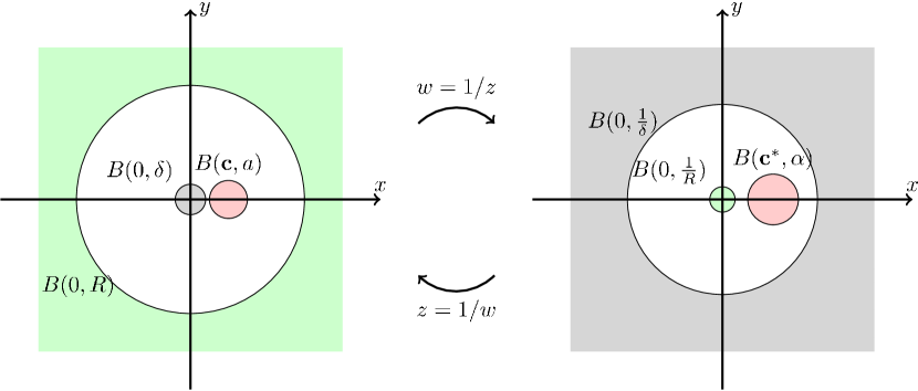
Figure 3: The regions of Theorem 2.1 (left) and their transforms under the Kelvin or inversion transformation (right). The device field is harmonic everywhere except in the gray areas, is close to minus the incident field in the red region and is close to zero in the green region.

Theorem 2.1

Let $a$, ${\bf c}$, $R$ and $\delta$ satisfy (22), then for any $\epsilon>0$ and any harmonic potential $u_{0}$, there exists a function $g_{0}:\mathbb{R}^{2}\to\mathbb{R}$ and a potential $u:\mathbb{R}^{2}\to\mathbb{R}$, satisfying

$$\left\{\begin{aligned} \varDelta u&=0,~{}\text{in $\mathbb{R}^{2}\setminus\overline{B(0,\delta)}$,}\\ u&=g_{0},~{}\text{on $\partial B(0,\delta)$,}\\ |u|&<\epsilon~{}\text{in $\mathbb{R}^{2}\setminus B(0,R)$,}\\ |u+u_{0}|&<\epsilon~{}\text{in $\overline{B({\bf c},a)}$.}\end{aligned}\right.$$ (23)

Proof

By applying the inversion (or Kelvin) transformation $\displaystyle w\doteq 1/z$, the geometry of problem (23) transforms as follows,

• $\mathbb{R}^{2}\setminus B(0,\delta)$ transforms to $B(0,1/\delta)$,

• $\mathbb{R}^{2}\setminus B(0,R)$ transforms to $B(0,1/R)$,

• $B({\bf c},a)$ transforms to $B({\bf c}^{*},\alpha)$, with

  $$\alpha=\frac{a}{|p^{2}-a^{2}|},~{}~{}{\bf c}^{*}=(\beta,0),~{}~{}\text{and}~{}~{}\beta=\frac{p}{p^{2}-a^{2}}.$$

The different regions and their transforms are illustrated in Fig. 3. Thus the problem (23) is equivalent to finding $\widetilde{g}_{0}$ and $\widetilde{u}$ such that

$$\left\{\begin{aligned} \varDelta\widetilde{u}&=0,~{}\text{in $B(0,1/\delta)$},\\ \widetilde{u}&=\widetilde{g}_{0},~{}\text{on $\partial B(0,1/\delta)$},\\ |\widetilde{u}|&<\epsilon,~{}\text{in $\overline{B(0,{1/R})}$},\\ |\widetilde{u}+\widetilde{u}_{0}|&<\epsilon,~{}\text{in $\overline{B({\bf c}^{*},\alpha)}$.}\end{aligned}\right.$$ (24)

Relating to the functions $g_{0}$ and $u_{0}$ from (23), we get $\widetilde{g}_{0}(z)=g_{0}(1/z)$ and $\widetilde{u}_{0}(z)=u_{0}(1/z)$, so that $\widetilde{u}_{0}$ is harmonic in the whole space except the origin. Next, we observe that the inversion transforms the necessary conditions (22) to

$$\frac{1}{R} <\beta-\alpha,~{}\text{the two balls $B(0,1/R)$ and $B({\bf c}^{*},\alpha)$ do not touch},$$ (25)

$$\beta+\alpha <\frac{1}{\delta},~{}\text{the two balls $B(0,1/\delta)$ and $B({\bf c}^{*},\alpha)$ do not touch}.$$

Let $\widetilde{U}_{0}$ be the analytic extension of $\widetilde{u}_{0}$ in $B({\bf c}^{*},\alpha)$, obtained with the harmonic conjugate such that $\widetilde{u}_{0}$ is the real part of $\widetilde{U}_{0}$. Because of analyticity of $\widetilde{U}_{0}$, we can approximate $\widetilde{U}_{0}$ with a polynomial $Q_{0}$ (e.g. by truncating the series expansion of $\widetilde{U}_{0}$) such that

$$|\widetilde{U}_{0}-Q_{0}|<\frac{\epsilon}{2}~{}\text{in $\overline{B({\bf c}^{*},\alpha)}$}.$$ (26)

This immediately yields the approximation for $\widetilde{u}_{0}$

$$|\widetilde{u}_{0}-q_{0}|<\frac{\epsilon}{2}~{}\text{in $\overline{B({\bf c}^{*},\alpha)}$},$$ (27)

where $q_{0}\doteq\Re(Q_{0})$, i.e., the real part of $Q_{0}$. Since $\widetilde{U}_{0}$ can be approximated arbitrarily well by a polynomial, it is enough to consider (24) when $\widetilde{u}_{0}$ is the real part of a polynomial, i.e.

$$\left\{\begin{aligned} \varDelta\widetilde{u}&=0,~{}\text{in $B(0,1/\delta)$},\\ \widetilde{u}&=\widetilde{g}_{0},~{}\text{on $\partial B(0,1/\delta)$},\\ |\widetilde{u}|&<\epsilon,~{}\text{in $\overline{B(0,1/R)}$},\\ |\widetilde{u}+q_{0}|&<\epsilon/2,~{}\text{in $\overline{B({\bf c}^{*},\alpha)})$}.\end{aligned}\right.$$ (28)

In other words, problem (28) is equivalent to finding a function $\widetilde{u}$, harmonic inside $B(0,1/\delta)$ that approximates $q_{0}$ well inside $B({\bf c}^{*},\alpha)$ but is practically zero in $B(0,1/R)$.

Let us now recall a classic result in harmonic approximation theory due to Walsh (see Gardiner (1995), page 8).

Lemma 1 (Walsh)

Let $K$ be a compact set in $\mathbb{R}^{2}$ such that $\mathbb{R}^{2}\setminus K$ is connected. Then for each function $w$, harmonic on an open set containing $K$, and for each $d>0$, there is a harmonic polynomial $q$ such that $|w-q|<d$ on $K$.

Walsh’s lemma implies the existence of a harmonic solution to problem (28). Indeed, from the design requirements (25) there exists $0<\xi\ll 1$ such that

$$\frac{1}{R}+\xi<\beta-\alpha-\xi.$$ (29)

Then applying Lemma 1 with $K=\overline{B(0,1/R)}\cup\overline{B({\bf c}^{*},\alpha)}$, we obtain that for an arbitrary small parameter $0<d\ll 1$ and for the function $w$ satisfying

$$w=\begin{cases}0&\text{ in $B(0,\frac{1}{R}+\xi)$},\\ -q_{0}&\text{ in $B({\bf c}^{*},\alpha+\xi)$},\end{cases}$$ (30)

there exists a harmonic polynomial $q$ such that $|q-w|<d$ on $K$. We conclude that there exists a harmonic solution to problem (28), which implies the statement of Theorem 2.1. ∎

2.3 Explicit polynomial solution in the
zero frequency regime

Although mathematically rigorous, the existence result of Theorem 2.1 (which follows from Walsh’s lemma) does not give an explicit expression for the required potential at the active device (antenna). In Guevara Vasquez et al (2009a) (see also Guevara Vasquez et al (2011c)) we give a polynomial solution to problem (24). Unfortunately the radius $a$ of the cloaked region in the polynomial solution of Guevara Vasquez et al (2009a, 2011c) is limited by the distance from the origin $p$ according to $a<(2+2\sqrt{2})^{-1}p$. Thus in Guevara Vasquez et al (2009a, 2011c) we can only cloak large objects if they are sufficiently far from the origin. Here we state a conjecture that extends our previous results Guevara Vasquez et al (2009a, 2011c) and that gives more freedom on the choice of the cloaked region location and size. This is supported by numerical evidence (see Figs. 4 and 5).

Conjecture 1

Let ${\bf c}^{*}=(\beta,0)$ be as in the proof of Theorem 2.1. For any $L>0$, any disk $S_{1}$ in the connected component containing the origin of the set

$$D_{\beta,L}\doteq\left\{{z\in\mathbb{C},~{}|z-\beta|^{L}|z|<\frac{\beta^{L+1}L^{L}}{(L+1)^{L+1}}}\right\},$$ (31)

any disk $S_{2}$ in the connected component of the set $D_{\beta,L}$ containing the point ${\bf c}^{*}$ and any $\epsilon>0$, there exists two positive integers $s$ and $n$ such that $|s/n-L|<\epsilon$ and the polynomial $P_{n,s}:\mathbb{C}\to\mathbb{C}$ defined by

$$P_{n,s}(z)=\left({1-\frac{z}{\beta}}\right)^{s}~{}\sum_{j=0}^{n-1}\left({\frac{z}{\beta}}\right)^{j}{s+j-1\choose j},$$ (32)

satisfies

$$|P_{n,s}-1|<\epsilon~{}\text{on $\partial S_{1}$}~{}~{}\text{and}~{}~{}|P_{n,s}|<\epsilon~{}\text{ on $\partial S_{2}$.}$$ (33)

Moreover the approximation property (33) is not satisfied when either $S_{1}$ or $S_{2}$ is not contained in $D_{\beta,L}$.

Remark 4

To see why we expect that the polynomial $P_{n,s}$ satisfies (33), notice that $z=\beta$ is a root of multiplicity $s$ of the polynomial $P_{n,s}$. From the Taylor expansion of $P_{n,s}$ around $z=\beta$, we can expect that $P_{n,s}\approx 0$ in a sufficiently small disk around $\beta$. (The symbol $\approx$ denotes an approximation with respect to the supremum norm.) Now the function

$$g(z)=\left[{\sum_{j=0}^{n-1}\left({\frac{z}{\beta}}\right)^{j}{s+j-1\choose j}}\right]-\left({1-\frac{z}{\beta}}\right)^{-s},$$

has a root of multiplicity $n$ at $z=0$, i.e. $g^{(k)}(0)=0$ for $k=0,\ldots,n-1$. This is because the sum in the definition of $g(z)$ corresponds to the first $n$ terms in the Taylor expansion around $z=0$ of $(1-z/\beta)^{-s}$. Thus by Leibniz rule, $z=0$ is a root of multiplicity $n$ of the polynomial $P_{n,s}-1=(1-z/\beta)^{s}g(z)$, and we can expect $P_{n,s}\approx 1$ in a sufficiently small disk around the origin. This suggests an alternative definition of $P_{n,s}$ as the unique Hermite interpolation polynomial (see e.g. Stoer and Bulirsch (2002)) satisfying:

$$P_{n,s}(0) =1,$$

$$P_{n,s}^{(k)}(0) =0,~{}~{}\text{for $k=1,\ldots,n-1$},$$

$$P_{n,s}^{(k)}(\beta) =0,~{}~{}\text{for $k=0,\ldots,s-1$}.$$

Remark 5

To motivate our belief that the region $D_{\beta,L}$ is the region of convergence of $P_{n,s}$ as $n\to\infty$ and $s\to\infty$ with $s/n\to L$, consider the special case where $L>0$ is an integer and $s=nL$. Then the last term in the sum (32) defining $P_{n,nL}(z)$ is

$$\left({1-\frac{z}{\beta}}\right)^{nL}\left({\frac{z}{\beta}}\right)^{n-1}{n(L+1)-1\choose n-1},$$

which diverges outside of $D_{\beta,L}$ as $n\to\infty$ because

$${n(L+1)-1\choose n-1}^{\frac{1}{n-1}}\to\frac{(L+1)^{L+1}}{L^{L}},~{}\text{as $n\to\infty$},$$

which follows from Stirling’s formula, see e.g. (Olver et al, 2010, §5.11). Therefore the region of divergence of $P_{n,Ln}$ contains the complement of $D_{\beta,L}$.

For some polynomial $Q_{0}$ we can deduce from (33) that

$$Q_{0}P_{n,s}-Q_{0}\approx 0~{}\text{on $\partial S_{1}$}~{}~{}\text{and}~{}~{}Q_{0}P_{n,s}-Q_{0}\approx-Q_{0}~{}\text{ on $\partial S_{2}$,}$$ (34)

Thus, by construction, the real part of $W=Q_{0}P_{n,s}-Q_{0}$ is a solution of (28) with $S_{1}=B(0,1/R)$ and $S_{2}=B({\bf c}^{*},\alpha)$. In the particular case when $n=s$ (i.e. $L=1$), Conjecture 1 was proved in Guevara Vasquez et al (2011c), see also Guevara Vasquez et al (2009a).

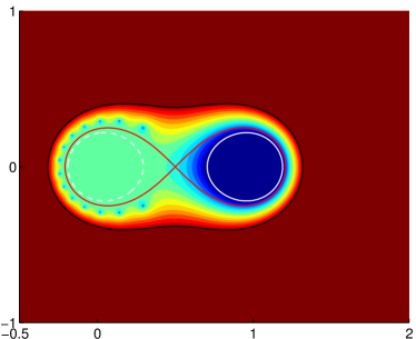
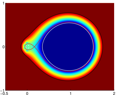
(a) $n=s=15$	(b) $n=5$, $s=25$

Figure 4: Contour plot for the polynomial $P_{n,s}$ with $\beta=1$. The solid white line is the level-set $|P_{n,s}(z)|=10^{-2}$, thus the cloaked region could be any disk inside this level-set. The dashed white line is the level-set $|P_{n,s}(z)-1|=10^{-2}$. The device field is small in any circle inside this level-set. The red curve is the boundary of $D_{\beta,L}$, the conjectured region of convergence of $P_{n,s}$ as both $n\to\infty$ and $s\to\infty$ with $s/n=1$ and $5$, respectively. (This is proved in the case $n=s$ in Guevara Vasquez et al (2011c).) The color scale is logarithmic from 0.01 (dark blue) to 100 (dark red), with light green representing 1.

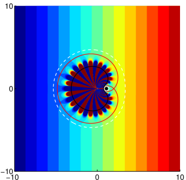
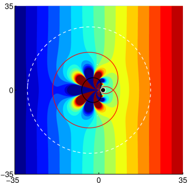
(a) $n=s=15$	(b) $n=5$, $s=25$

Figure 5: Real part of the total field with the cloaking device active, incident field $u_{0}(x,y)=x$ and $\beta=1$. The solid white, dashed white and red lines are the inversion (Kelvin) transforms of their counterparts in Fig. 4. The small black scatterer inside the cloaked region is an almost resonant disk centered at $(p,0)$ with radius $r$ and dielectric constant $\epsilon$ given by: (a) $p=1.1$, $r=0.2$ and $\epsilon=-0.99$; (b) $p=1.7$, $r=0.9$ and $\epsilon=-0.998$. In (a) the color scale is linear from -10 (dark blue) to 10 (dark red). In (b) the scale is linear from -35 to 35.

In Fig. 4 we present a contour plot of the polynomial $P_{n,s}$ when $\beta=1$ for different values of $n$ and $s$. The region bounded by the peanut shaped red curve represents the conjectured domain of convergence $D_{\beta,L}$ of the functions $P_{n,s}$ when $n\rightarrow\infty$, $s\rightarrow\infty$ and $s/n\rightarrow L$. In the left side of $D_{\beta,L}$, $P_{n,s}$ is conjectured to converge to one, while in the right side of $D_{\beta,L}$, $P_{n,s}$ is conjectured to converge to zero. The area within the solid white circle on the right represents the region to be cloaked and the area within the dashed white circle in the left represents the location of the observer. We now present an active cloak design based on Conjecture 1.

Remark 6

Let $u_{0}$ be an a priori determined incoming harmonic potential. Let $n$ and $s$ be such that the real part of $W=Q_{0}P_{n,s}-Q_{0}$ is a solution of (28) (recall $Q_{0}$ is a polynomial approximation of $\widetilde{U}_{0}$ in $B({\bf c}^{*},\alpha)$). Let $S$ be a bounded region in the complex plane compactly including the two disks $S_{1}=B(0,{\frac{1}{R}})$ and $S_{2}=B({\bf c}^{*},\alpha)$. Then, the cloaking strategy we propose consists of an active device (antenna) located inside $B(0,\delta)$ and capable of generating a potential equal to the real part of $W({1\over z})$ on the set $\{z\in\mathbb{C},{1\over z}\in\partial S\}$. By (27), the total potential in the original physical configuration (the field from the antenna plus $u_{0}$) is well approximated by the real part of $(W+Q_{0})(1/z)$ which ensures an almost zero field region in $B({\bf c},a)$ with negligible perturbations on the field outside $B(0,R)$.

Fig. 5 illustrates how the cloaking device (represented by the solid black curve) works after applying the back-inversion to the configurations presented in Fig. 4. Here the incident field is $u_{0}(x,y)=x$ and the objects we want to hide are almost resonant disks. Clearly, the active device generates the necessary field to cancel the field in the cloaked region while having a very small effect in the far field (outside the white dashed circle). With a polynomial of the same degree, when $s=5n$ (Fig. 5(b)) we can hide an object roughly four times larger than when $s=n$ (Fig. 5(a)). Thus using the polynomials $P_{n,s}$ allows us to cloak large objects without restrictions on the distance from the origin $\beta$ as was the case in Guevara Vasquez et al (2009a, 2011c). The disadvantage is that cloaking is enforced on $\partial B(0,R)$ (dotted white line in Fig. 5) with a larger $R$ in the asymmetric $L>1$ case than in the symmetric $L=1$ case. For example to get a device field such that $|u|<10^{-2}$, $R$ needs to be roughly five times larger when $s=5n$ (Fig. 5(b)) than when $s=n$ (Fig. 5(a)).

2.4 Extensions and applications

We now extend the previous results to the case of an incoming field having sources in $\mathbb{R}^{2}\setminus\overline{B(0,R)}$.

Remark 7

The case studied in Theorem 2.1 (with an explicit solution in Conjecture 1) corresponds to an incoming field $u_{0}$ generated by a source located at infinity. The more general case corresponding to an incoming field having sources in $\mathbb{R}^{2}\setminus\overline{B(0,R)}$ can be treated similarly. Indeed, the problem remains to find $g_{0}$ and $u$ satisfying (23), or equivalently $\widetilde{g}_{0}$ and $\widetilde{u}$ satisfying (24) where inside $B(0,{1/R})$, $\widetilde{u}_{0}(z)=u_{0}(1/z)$ is harmonic. We can still approximate its analytic extension $\widetilde{U}_{0}$ by a polynomial in $B({\bf c}^{*},\alpha)$ and the proof goes as in Theorem 2.1.

Although our main focus here is cloaking, the same ideas can be applied to illusion optics, where one wants to conceal an object by imitating the response (scattering) of a completely different object.

Remark 8

Let $u_{1}$ be the response of an object we wish to imitate, i.e. an arbitrary potential harmonic in a set $D_{1}\subset\mathbb{R}^{2}$ such that $\mathbb{R}^{2}\setminus B(0,R)\Subset D_{1}$. Assuming the same notations as before, for any (known a priori) probing field $u_{0}$, harmonic in $\mathbb{R}^{2}$, there exists a function $g\in C(\partial B(0,\delta))$ so that the field $u$ generated by the active device (antenna) located in $B(0,\delta)$ satisfies:

1. The total field $u+u_{0}$ is very small in the cloaked region $B({\bf c},a)$.

2. The device field $u$ is close to $u_{1}$ in $\mathbb{R}^{2}\setminus B(0,R)$.

Remark 8 follows from the inversion (Kelvin) transform and Lemma 1 by using an argument similar to the proof of Theorem 2.1. Using ideas similar to those in Remark 7, the result of Remark 8 can be generalized to the case of an incoming field with sources in $\mathbb{R}^{2}\setminus\overline{B(0,R)}$.

To illustrate Remark 8 assume that the field $u_{1}$ is chosen to be the response field of an inhomogeneity ${\cal I}$ when probed with the incident field $u_{0}$. Then Remark 8 means that when probing with the field $u_{0}$, an observer located in the far field detects the inhomogeneity ${\cal I}$ regardless of the inclusion inside $B({\bf c},a)$ and without detecting the active illusion device. This creates the illusion that the object inside $B({\bf c},a)$ is the inhomogeneity ${\cal I}$.

3 Active exterior cloaking for the Helmholtz equation in
three dimensions

Previously in Guevara Vasquez et al (2009a, b) we designed cloaking devices generating fields close to minus the incident field in the region to be cloaked and vanishing far away from the devices. Miller Miller (2006) proposed an active cloak based on Green’s identities: a single and double layer potential is applied to the boundary of the cloaked region to cancel out the incident field inside the cloaked region, while not radiating waves. The idea of using Green’s identities to cancel out waves in a region is well known in acoustics (see e.g. Ffowcs Williams (1984); Malyuzhinets (1964); Jessel and Mangiante (1972)). Jessel and Mangiante Jessel and Mangiante (1972) showed that it is possible to achieve a similar effect to Green’s identities (and thus cloaking) by replacing the single and double layer potentials on a surface by a source distribution in a neighborhood of the surface. What makes our approach different is that the cloaking devices are multipolar sources exterior to the cloaked region and thus do not completely enclose the cloaked region. In Guevara Vasquez et al (2009a, b) the cloaking devices are determined by solving numerically a least-squares problem with linear constraints. Our cloaking approach easily generalizes to several frequencies Guevara Vasquez et al (2009b) but requires a priori knowledge of the incident field. Zheng, Xiao, Lai and Chan Zheng et al (2010) used the same principle to achieve illusion optics Lai et al (2009) with active devices, i.e. making an object appear as another one. Then in Guevara Vasquez et al (2011b) we showed Green’s identity can be used to design devices which can cloak or give the illusion of another object, i.e. achieving an effect similar to the active devices in Guevara Vasquez et al (2009a, b); Zheng et al (2010). The single and double layer potential needed to reproduce a smooth field inside a region while being zero outside is given by Green’s identity and can be replaced by a few multipolar sources using addition formulas for spherical outgoing waves. If in addition we want to imitate the scattered field from an object as in Zheng et al (2010), a similar procedure applies.

The active cloaking devices we designed in Guevara Vasquez et al (2009a, b, 2011b) are two dimensional. Here we extend the result in Guevara Vasquez et al (2011b) to the Helmholtz equation in three dimensions. The wave pressure field $u({\bf x})$ solves the Helmholtz equation,

$$\varDelta u+k^{2}u=0,~{}~{}\text{for ${\bf x}\in\mathbb{R}^{3}$},$$

where $k=2\pi/\lambda$ is the wavenumber, $\lambda=2\pi c/\omega$ is the wavelength, $c$ is the wave propagation speed (assumed to be constant) and $\omega$ is the angular frequency. Recall for future reference that the radiating Green’s function for the Helmholtz equation in three dimensions is

$$G({\bf x},{\bf y})=\frac{\exp[ik\left|{{\bf x}-{\bf y}}\right|]}{4\pi\left|{{\bf x}-{\bf y}}\right|}$$ (35)

Another underlying assumption is that the frequency $\omega$ is not a resonant frequency of the scatterer we wish to hide.

3.1 Green’s formula cloak

As pointed out by Miller Miller (2006) it is possible to cloak an object inside a bounded region $D\in\mathbb{R}^{3}$ from an incident wave (probing field) $u_{i}$ by generating a cloaking device field using monopole and dipole sources (single and double layer potential) on $\partial D$. The device field $u_{d}$ can be defined using Green’s formula

$$u_{d}({\bf x}) =\int_{\partial D}\mathrm{d}S_{\bf y}\left\{{-({\bf n}({\bf y})\cdot\nabla_{\bf y}u_{i}({\bf y}))G({\bf x},{\bf y})+u_{i}({\bf y}){\bf n}({\bf y})\cdot\nabla_{\bf y}G({\bf x},{\bf y})}\right\}$$ (36)

$$=\begin{cases}-u_{i}({\bf x}),&\text{if ${\bf x}\in D$}\\ 0,&\text{otherwise},\end{cases}$$

so that the total field $u_{i}+u_{d}$ is a solution to Helmholtz equation for ${\bf x}\notin\partial D$ that vanishes inside $D$ while being indistinguishable form $u_{i}$ outside $D$. Since the waves reaching a scatterer inside the cloaked region $D$ are practically zero, the resulting scattered field is also practically zero. For clarity we assume the region $D$ is a polyhedron. The arguments we give here can be easily modified for other domains with Lipschitz boundary, as Green’s identity (36) is valid for these domains Evans and Gariepy (1992).

Remark 9

The Green representation formula (36) requires that $u_{i}$ be a $C^{2}$ solution to the Helmholtz equation inside $D$. A similar identity holds when $u_{i}$ is a $C^{2}$ radiating solution to the Helmholtz equation outside $D$. In this case, the device field $u_{d}$ vanishes inside $D$ and is identical to $-u_{i}$ outside $D$. The exterior cloak we present here can in principle be used to conceal a known active source and possibly accompanying scatterers inside $D$. If the radiating wave $u_{i}$ is taken to be the scattered field from a known object, the same principle can be used for illusion optics Lai et al (2009); Zheng et al (2010).

3.2 Active exterior cloak

The main idea here is to achieve a similar effect to the Green’s identity cloak but without completely surrounding the cloaked region by monopoles and dipoles on $\partial D$. We “open the cloak” by replacing the single and double layer potential on each face $\partial D_{l}$ of $\partial D$ by a corresponding multipolar device located at some point ${\bf x}_{l}$. Each device produces a linear combination of outgoing spherical waves of the form

$$u_{d}({\bf x})=\sum_{l=1}^{n_{dev}}\sum_{n=0}^{\infty}\sum_{m=-n}^{n}b_{l,n,m}V_{n}^{m}({\bf x}-{\bf x}_{l}),$$ (37)

where $n_{dev}$ is the number of devices (or faces of $\partial D$) and $V_{n}^{m}({\bf x})$ is a radiating, spherical wave defined for ${\bf x}\neq 0$ by

$$V_{n}^{m}({\bf x})=h_{n}^{(1)}(k|{\bf x}|)Y_{n}^{m}(\widehat{{\bf x}}).$$

Here $h_{n}^{(1)}(t)$ is a spherical Hankel function of the first kind (see e.g. (Olver et al, 2010, §10.47)) and $Y_{n}^{m}(\widehat{{\bf x}})$ is a spherical harmonic evaluated at the point $\widehat{{\bf x}}\equiv{\bf x}/\left|{{\bf x}}\right|$ of the unit sphere $S(0,1)$. In spherical coordinates, the spherical harmonics we use are defined as in (Colton and Kress, 1998, §2.3) by

$$Y_{n}^{m}(\theta,\phi)=\sqrt{\frac{2n+1}{4\pi}\frac{(n-\left|{m}\right|)!}{(n+\left|{m}\right|)!}}P_{n}^{\left|{m}\right|}(\cos\theta)e^{im\phi},$$ (38)

where the elevation angle is $\theta\in[0,\pi]$ and the azimuth angle is $\phi\in[0,2\pi]$. Here $P_{n}^{\left|{m}\right|}(t)$ are the associated Legendre functions

$$P_{n}^{m}(t)=(1-t^{2})^{m/2}\frac{d^{m}P_{n}(t)}{dt^{m}},$$

defined for $n=0,1,2,\ldots$ and $m=0,1,\ldots,n$ in terms of the Legendre polynomials $P_{n}$ of degree $n$ with normalization $P_{n}(1)=1$. The definition (38) ensures that the spherical harmonics $Y_{n}^{m}$ have unit $L^{2}(S(0,1))$ norm.

The main tool to replace the fields generated by a face is the addition formula (see e.g. Theorem 2.10 in Colton and Kress (1998))

$$G({\bf x},{\bf y})=ik\sum_{n=0}^{\infty}\sum_{m=-n}^{n}V_{n}^{m}({\bf x})\overline{U_{n}^{m}({\bf y})}$$ (39)

which means we can mimic a point source located at ${\bf y}$ by a multipolar source located at the origin. The coefficients in the multipolar expansion are values of entire spherical waves

$$U_{n}^{m}({\bf x})=j_{n}(k|{\bf x}|)Y_{n}^{m}(\widehat{{\bf x}}),$$

where $j_{n}(t)$ are spherical Bessel functions (Olver et al, 2010, §10.47). The series in the multipolar expansion (39) converges uniformly on compact sets of $|{\bf x}|>|{\bf y}|$.

We are now ready to state the main result of this section.

Theorem 3.1

Multipolar sources located at the points ${\bf x}_{l}\notin\partial D$, $l=1,\ldots,n_{dev}$ can be used to reproduce the Green’s formula cloak outside of the region

$$A=\bigcup_{l=1}^{n_{dev}}B\left({{\bf x}_{l},\sup_{{\bf y}\in\partial D_{l}}|{\bf y}-{\bf x}_{l}|}\right),$$

where $B({\bf x},r)$ is the closed ball of radius $r$ centered at ${\bf x}$. The coefficients $b_{l,n,m}$ in (37) such that $u_{d}^{(ext)}({\bf x})=u_{d}({\bf x})$ for ${\bf x}\notin A$ are

$$b_{l,n,m}=ik\int_{\partial D_{l}}\mathrm{d}S_{\bf y}\Bigl{\{} (-{\bf n}({\bf y})\cdot\nabla_{\bf y}u_{i}({\bf y}))\overline{U_{n}^{m}({\bf y}-{\bf x}_{l})}$$ (40)

$$+u_{i}({\bf y}){\bf n}({\bf y})\cdot\nabla_{\bf y}\overline{U_{n}^{m}({\bf y}-{\bf x}_{l})}\Bigr{\}}.$$

Moreover the convergence of (37) is uniform on compact sets outside $A$.

Proof

Splitting the integral in (36) into integrals over each of the faces $\partial D_{l}$ of the polyhedron $\partial D$ and applying the addition theorem (39) with center at the corresponding ${\bf x}_{l}$ we obtain:

$$u_{d}({\bf x})=ik\sum_{l=1}^{n_{dev}}\int_{\partial D_{l}}\mathrm{d}S_{\bf y} (-{\bf n}({\bf y})\cdot\nabla_{\bf y}u_{i}({\bf y}))\sum_{n=0}^{\infty}\sum_{m=-n}^{n}V_{n}^{m}({\bf x}-{\bf x}_{l})\overline{U_{n}^{m}({\bf y}-{\bf x}_{l})}$$ (41)

$$+u_{i}({\bf y}){\bf n}({\bf y})\cdot\nabla_{\bf y}\sum_{n=0}^{\infty}\sum_{m=-n}^{n}V_{n}^{m}({\bf x}-{\bf x}_{l})\overline{U_{n}^{m}({\bf y}-{\bf x}_{l})}.$$

The result (40) follows for ${\bf x}\notin A$ by switching the order of the sum and the integral in (41). For the first term in the integrand of (41), this switch is justified by the uniform convergence of the series (39) (for all devices) in compact sets outside of $A$.

For the second term in the integrand of (41), we shall show that the series converges uniformly on compact sets outside $A$, so it is also valid to switch the integral and the series in (41). To see the uniform convergence, it is useful to split the products $V_{n}^{m}({\bf x}-{\bf x}_{l})\nabla_{\bf y}\overline{U_{n}^{m}({\bf y}-{\bf x}_{l})}$ into two terms corresponding to the two terms in the gradient

$$\nabla_{\bf y}U_{n}^{m}({\bf y}) =k\widehat{{\bf y}}j_{n}^{\prime}(k\left|{{\bf y}}\right|)Y_{n}^{m}(\widehat{{\bf y}}) +j_{n}(k\left|{{\bf y}}\right|)\frac{\left|{{\bf y}}\right|^{2}I-{\bf y}{\bf y}^{T}}{\left|{{\bf y}}\right|^{3}}(\nabla Y_{n}^{m})(\widehat{{\bf y}})$$ (42)

$$=g^{(1)}_{n,m}({\bf y}) +g^{(2)}_{n,m}({\bf y}),$$

where $I$ is the $3\times 3$ identity matrix.

For the series involving the first term in the gradient (42) we bound with the triangle and Cauchy-Schwarz inequalities:

$$\left|{\sum_{m=-n}^{n}V_{n}^{m}({\bf x}-{\bf x}_{l})\overline{g^{(1)}_{n,m}({\bf y}-{\bf x}_{l})}}\right|$$

$$\leq k\left|{h_{n}^{(1)}(k\left|{{\bf x}-{\bf x}_{l}}\right|)j^{\prime}_{n}(k\left|{{\bf y}-{\bf x}_{l}}\right|)}\right|\left({\sum_{m=-n}^{n}\left|{Y_{n}^{m}(\widehat{{\bf x}-{\bf x}_{l}})}\right|^{2}}\right)^{\frac{1}{2}}\left({\sum_{m=-n}^{n}\left|{Y_{n}^{m}(\widehat{{\bf y}-{\bf x}_{l}})}\right|^{2}}\right)^{\frac{1}{2}}.$$

Using the summation theorem for spherical harmonics (see e.g. Theorem 2.8 in Colton and Kress (1998))

$$\sum_{m=-n}^{n}\left|{Y_{n}^{m}(\widehat{{\bf y}})}\right|^{2}=\frac{2n+1}{4\pi},\text{for any $\widehat{{\bf y}}\in S(0,1)$ and $n=0,1,\ldots$,}$$ (43)

we get the estimate:

$$\left|{\sum_{m=-n}^{n}V_{n}^{m}({\bf x}-{\bf x}_{l})\overline{g^{(1)}_{n,m}({\bf y}-{\bf x}_{l})}}\right|$$ (44)

$$\leq k\left|{h_{n}^{(1)}(k\left|{{\bf x}-{\bf x}_{l}}\right|)j^{\prime}_{n}(k\left|{{\bf y}-{\bf x}_{l}}\right|)}\right|\frac{2n+1}{4\pi}$$

$$={\cal O}\left({\frac{\left|{{\bf y}-{\bf x}_{l}}\right|^{n-1}}{\left|{{\bf x}-{\bf x}_{l}}\right|^{n+1}}}\right),$$

for large $n\to\infty$. The last equality comes from the asymptotic expansion of Bessel functions for fixed $t>0$ and large order $n$, (see e.g. (Olver et al, 2010, §10.19))

$$\left|{j_{n}^{\prime}(t)}\right|={\cal O}(t^{n-1})~{}~{}\text{and}~{}~{}\left|{h_{n}^{(1)}(t)}\right|={\cal O}(t^{-n-1}).$$

For the series involving the second term in the gradient (42) we bound the sums

$$\left|{\sum_{m=-n}^{n}V_{n}^{m}({\bf x}-{\bf x}_{l})\overline{g^{(2)}_{n,m}({\bf y}-{\bf x}_{l})}}\right|$$

$$\leq 2\left|{h_{n}^{(1)}(k\left|{{\bf x}-{\bf x}_{l}}\right|)\frac{j_{n}(k\left|{{\bf y}-{\bf x}_{l}}\right|)}{\left|{{\bf y}-{\bf x}_{l}}\right|}}\right|\left({\sum_{m=-n}^{n}\left|{Y_{n}^{m}(\widehat{{\bf x}-{\bf x}_{l}})}\right|^{2}}\right)^{\frac{1}{2}}\left({\sum_{m=-n}^{n}\left|{(\nabla Y_{n}^{m})(\widehat{{\bf y}-{\bf x}_{l}})}\right|^{2}}\right)^{\frac{1}{2}}.$$

Using the summation theorem for spherical harmonics (43) and their gradients (see e.g. (6.56) in Colton and Kress (1998)),

$$\sum_{m=-n}^{n}\left|{(\nabla Y_{n}^{m})(\widehat{{\bf y}})}\right|^{2}=\frac{n(n+1)(2n+1)}{4\pi},~{}~{}\text{for any $\widehat{{\bf y}}\in S(0,1)$},$$ (45)

we get the asymptotic

$$\left|{\sum_{m=-n}^{n}V_{n}^{m}({\bf x}-{\bf x}_{l})\overline{g^{(2)}_{n,m}({\bf y}-{\bf x}_{l})}}\right|$$ (46)

$$\leq 2\left|{h_{n}^{(1)}(k\left|{{\bf x}-{\bf x}_{l}}\right|)\frac{j_{n}(k\left|{{\bf y}-{\bf x}_{l}}\right|)}{\left|{{\bf y}-{\bf x}_{l}}\right|}}\right|\left({\frac{2n+1}{4\pi}}\right)^{\frac{1}{2}}\left({\frac{n(n+1)(2n+1)}{4\pi}}\right)^{\frac{1}{2}}$$

$$={\cal O}\left({\frac{\left|{{\bf y}-{\bf x}_{l}}\right|^{n-1}}{\left|{{\bf x}-{\bf x}_{l}}\right|^{n+1}}}\right).$$

Here we have used that for $t>0$ fixed and as $n\to\infty$, (see e.g. (Olver et al, 2010, §10.19))

$$\left|{j_{n}(t)}\right|={\cal O}(t^{n})~{}~{}\text{and}~{}~{}\left|{h_{n}^{(1)}(t)}\right|={\cal O}(t^{-n-1}).$$

The estimates (44) and (46) give uniformly convergent majorants for the series in the second term of (41), since when ${\bf x}\notin A$ we have $\left|{{\bf y}-{\bf x}_{l}}\right|<\left|{{\bf x}-{\bf x}_{l}}\right|$, for $l=1,\ldots,n_{dev}$. The proof is now completed. ∎

3.3 A family of exterior cloaks with four devices

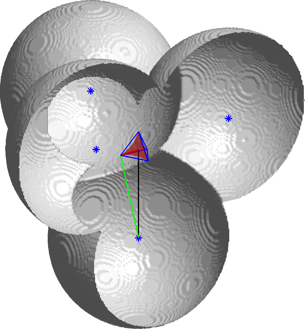
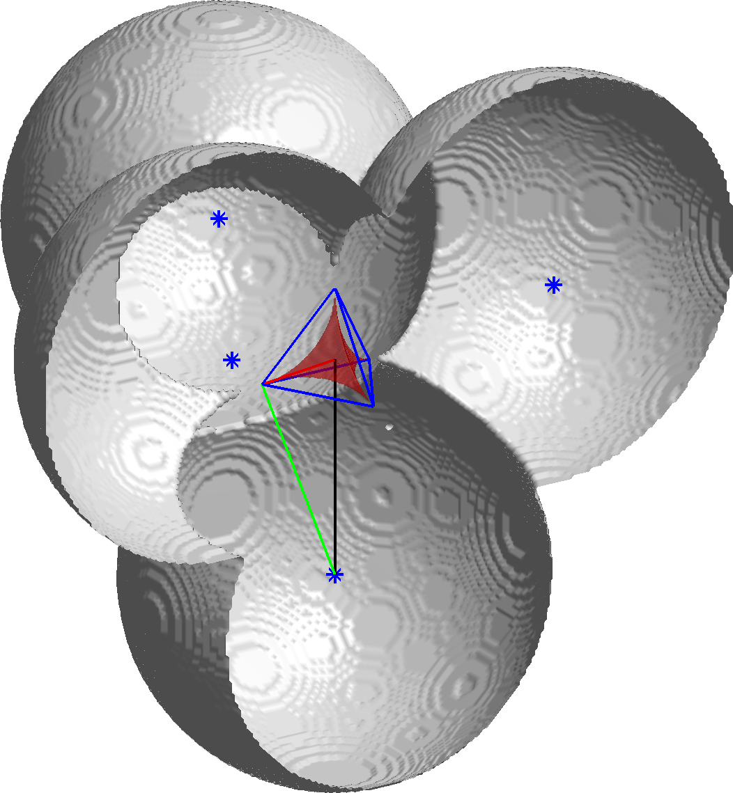
(a) suboptimal, $\sigma=\delta/5$	(b) optimal, $\sigma=\delta/3$

Figure 6: The configuration for the tetrahedron based cloak of Sect. 3.3. The distance in red is the radius $\sigma$ of the circumsphere to the tetrahedron $D$. The distance in black is the distance $\delta$ from the origin to a device. The distance $r(\sigma,\delta)$ (in green) is the distance from a device to the closest vertex of $D$. The exterior surface of the region $A$ of Theorem 3.1 is in grey and has been cut to reveal the cloaked region $D\setminus A$ in red. The four devices are shown with stars.

Nothing in Theorem 3.1 guarantees that the cloaked region $D\setminus A$ is non-empty. We show here how to construct a family of cloaks with non-empty $D\setminus A$ based on Green’s identities applied to a regular tetrahedron $D$. We also determine what is the position of the devices that gives the largest cloaked region within this family.

Consider a regular tetrahedron with circumsphere $S(0,\sigma)$ and vertices ${\bf a}_{1},\ldots,{\bf a}_{4}$. We locate the devices ${\bf x}_{1},\ldots,{\bf x}_{4}$ on $S(0,\delta)$, with $\delta>\sigma$, such that ${\bf x}_{l}$ replaces the face opposite to vertex ${\bf a}_{l}$, that is ${\bf x}_{l}$ and ${\bf a}_{l}$ are on opposite sides of the plane formed by the face of the tetrahedron not containing ${\bf a}_{l}$. For simplicity we also require that ${\bf x}_{l}-{\bf a}_{l}$ is normal to this plane. The configuration is sketched in Fig. 6. Simple geometric arguments show that the radii of the balls that define the region $A$ are all equal to

$$r(\sigma,\delta)=\left({\left({\sigma-\frac{\delta}{3}}\right)^{2}+\frac{8}{9}\delta^{2}}\right)^{\frac{1}{2}}.$$ (47)

Moreover the radius of the largest sphere fitting inside the cloaked region is

$$r_{\text{eff}}(\sigma,\delta)=\delta-r(\sigma,\delta).$$ (48)

For fixed $\delta$, the largest possible cloaked region is obtained when $\sigma=\delta/3$ which corresponds to the case when every triplet of balls in the definition of region $A$ touch at a vertex ${\bf a}_{l}$ of the tetrahedron. Thus for fixed $\delta$, the largest sphere we can fit inside the cloaked region has radius,

$$r_{\text{eff}}^{*}=\left({1-\frac{2\sqrt{2}}{3}}\right)\delta\approx 0.057\delta.$$ (49)

3.4 Numerical experiments

We report in Fig. 7 simulations of this cloaking method with the setup described in Sect. 3.3. The incident field we take is the plane wave $u_{i}({\bf x})=\exp[ik\widehat{{\bf k}}\cdot{\bf x}]$ with direction vector $\widehat{{\bf k}}=[1,1,1]/\sqrt{3}$. We first compute the device field of Theorem 3.1 by truncating the sum in $n$ of (37) to $n\leq N$. Throughout our numerical experiments we determine $N$ with the heuristic (found by numerical experimentation)

$$N(\delta)=\lceil{1.5k\delta}\rceil,$$ (50)

where $\lceil{x}\rceil$ is the smallest integer larger than or equal to $x$. The integrals in (40) were evaluated with a simple quadrature rule that is exact for piecewise linear functions on a uniform triangulation of the faces of the tetrahedron $D$, we chose the number of quadrature points so that there are at least eight points per wavelength. The scattered field by a ball was computed by first evaluating the incident field (or device field depending on the case) on a grid with equal number of points in $\phi$ and $\theta$ and then finding its first few spherical harmonic decomposition coefficients using the sampling theorem Driscoll and Healy (1994).

As can be seen in the first row of Fig. 7 the device field $u_{d}$ is virtually zero far from $A$ while being close to the incident field in the cloaked region $D\setminus A$. In the second and third rows of Fig. 7 we display the total field in the presence of a sound-soft (homogeneous Dirichlet boundary condition) ball centered at the origin and of radius $3r_{\text{eff}}^{*}(\delta)$ (i.e. a larger scatterer than what we expected from Sect. 3.3). The scattered field from the ball reveals the ball’s position when the devices are inactive (third row). The scattered field is essentially suppressed when the cloaking devices are active (second row), as the field is indistinguishable from a plane wave far from $A$.

Since as $t\to 0$, $h_{n}^{(1)}(t)={\cal O}(t^{-n-1})$ (see e.g. (Olver et al, 2010, §10.52)), we expect the device field $u_{d}$ to blow up as we get close to the device locations ${\bf x}_{l}$. This blow up corresponds to the “urchins” in the first and second rows of Fig. 7 where even with the truncation of the series (37), we observe very large wave amplitudes which would be hard to realize in practice. Fortunately we can enclose the regions with very large fields by a surface and apply Green’s formula (36) to replace these large fields by (hopefully) more manageable single and double layer potentials on the surface of some “extended” cloaking devices.

We illustrate these “extended” devices in Fig. 8 where we display the level sets where the device field amplitude is 5 (or 100) times the amplitude of the incident field. At least for the particular configuration ($\delta=6\lambda$) considered in Fig. 8, these surfaces resemble spheres surrounding each device location ${\bf x}_{l}$. The “extended” devices still leave the cloaked region (in red in Fig. 8) communicating (connected) with the background medium. This is why we call our cloaking method “exterior cloaking”.

We also consider the extended devices for larger values of $\delta$ in Fig. 9. Here we look at the cross-section of the extended devices on $S(0,\sigma)$, which in the construction of Sect. 3.3 is the circumsphere to the tetrahedron $D$. In the optimal case $\delta=3\sigma$, the predicted cloaked region $D\setminus A$ and the exterior $\mathbb{R}^{3}\setminus A$ meet on $S(0,\sigma)$ at the vertices of the tetrahedron $D$. We see that the extended devices (in black in Fig. 9) grow as $\delta$ increases, and leave gorges communicating the cloaked region with the exterior. The centers of the gorges appear to agree with the vertices of the tetrahedron $D$. The percentage area of $S(0,\sigma)$ that is not covered by the cross-section of the extended devices on $S(0,\sigma)$ is also quantified in Fig. 10(b). Since the relative area of the openings appears to decrease monotonically with $\delta/\lambda$, Fig. 10(b) suggests the gorges close for large enough $\delta/\lambda$. Further investigation is needed to find out whether the shrinking openings in the cloak is due to our choice of $N$ with heuristic (50).

Finally we give in Fig. 10(a) quantitative measures of the cloak performance for different values of $\delta$. These measures show that the device field is close to minus the incident field inside the cloaked region and that it is very small outside of the cloaked region.

	$z=-2\sigma$	$z=-\sigma$	$z=0$	$z=\sigma$	$z=2\sigma$
$u_{d}$
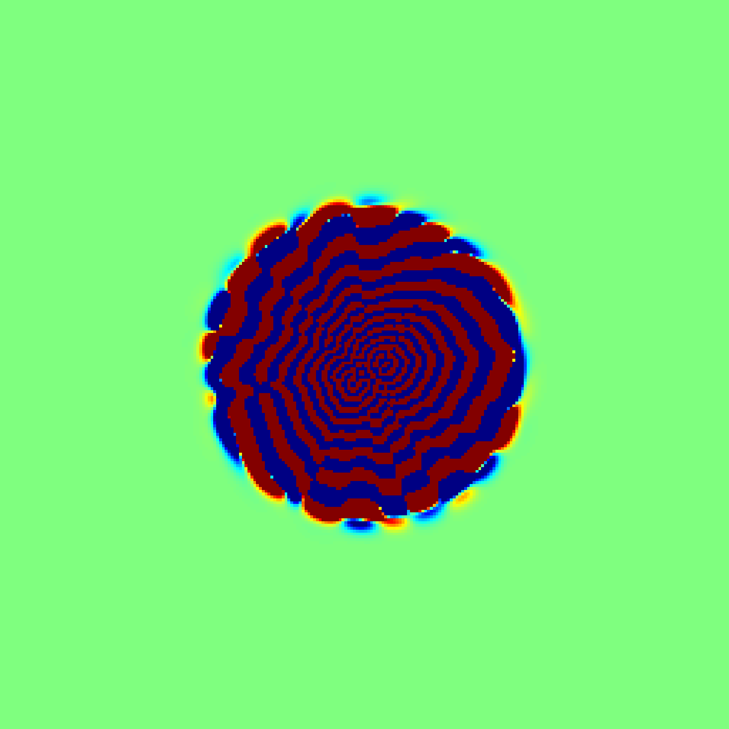
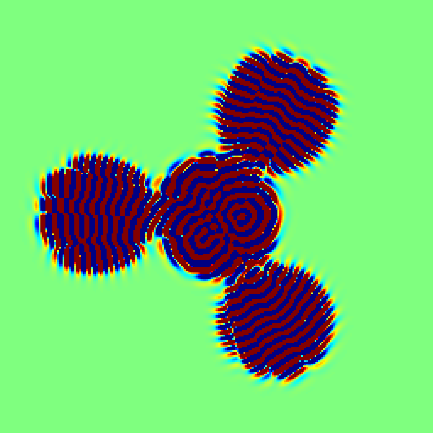
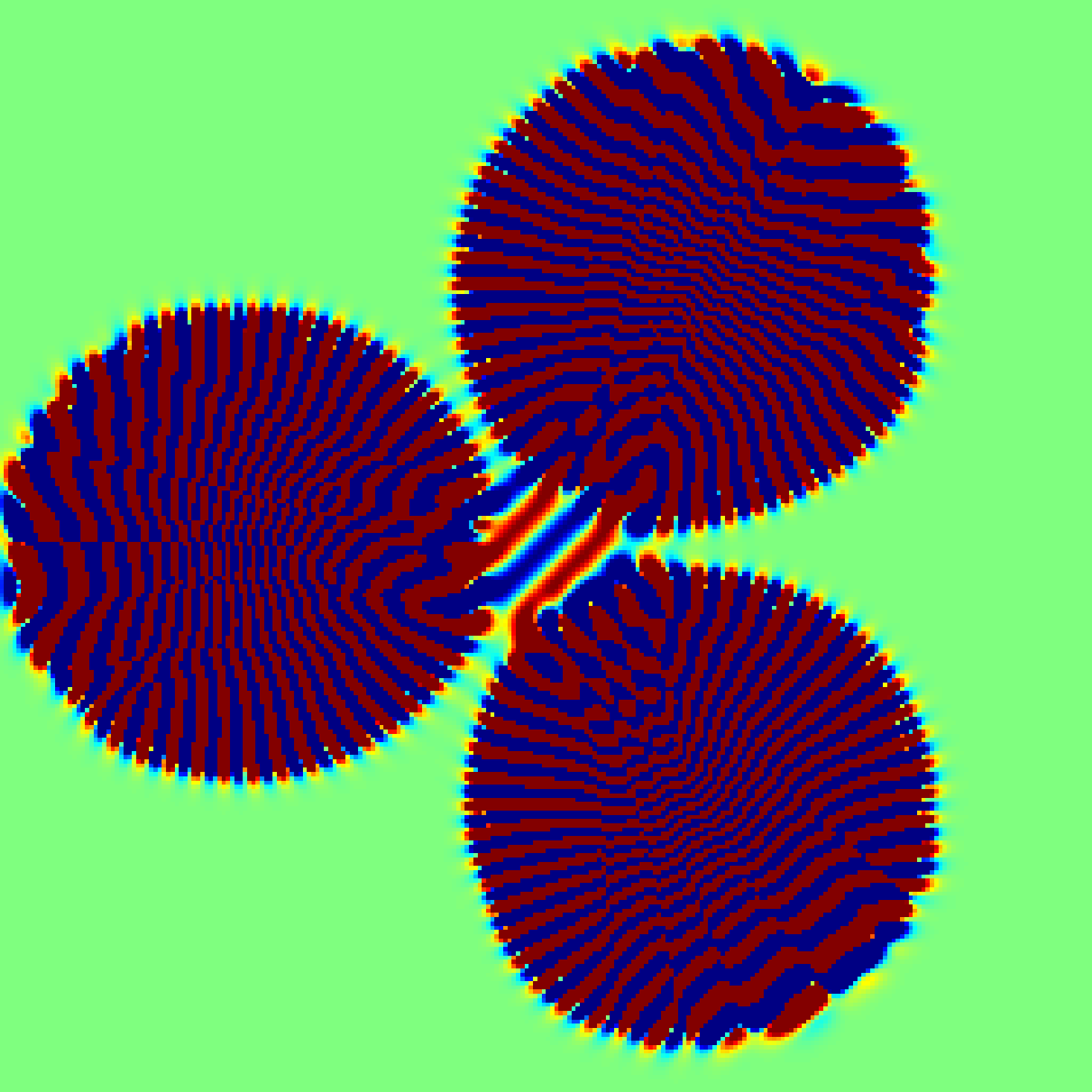
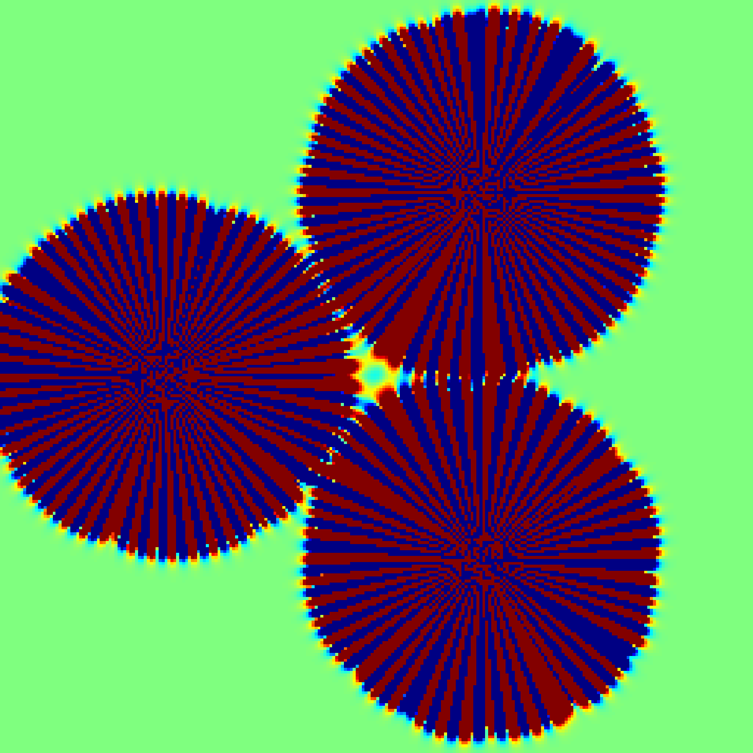
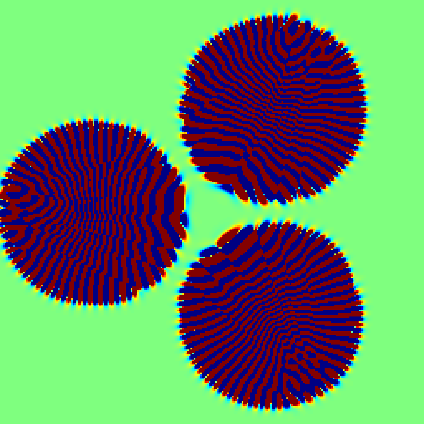
$u_{tot}$ (active)
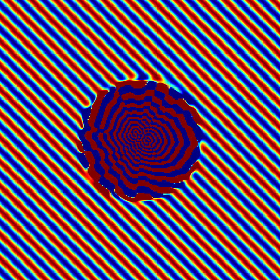
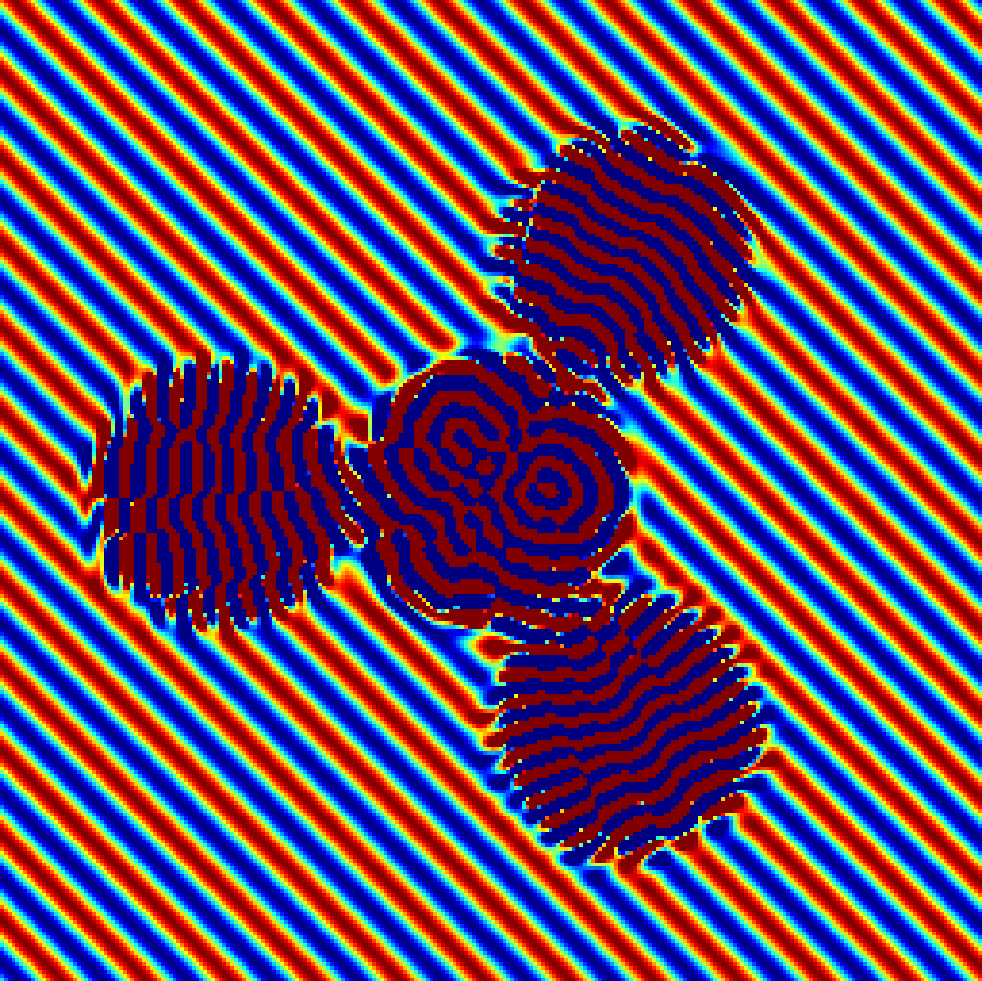
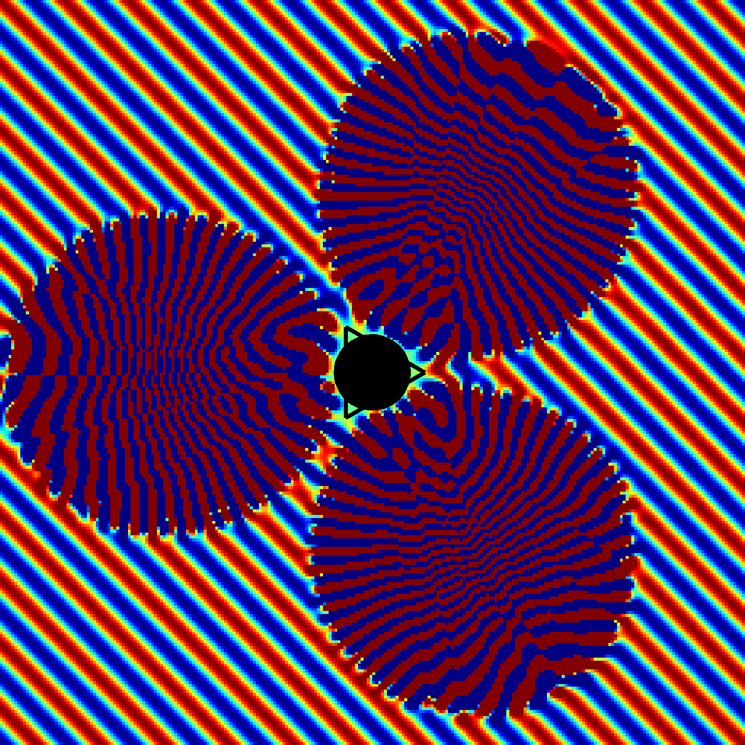
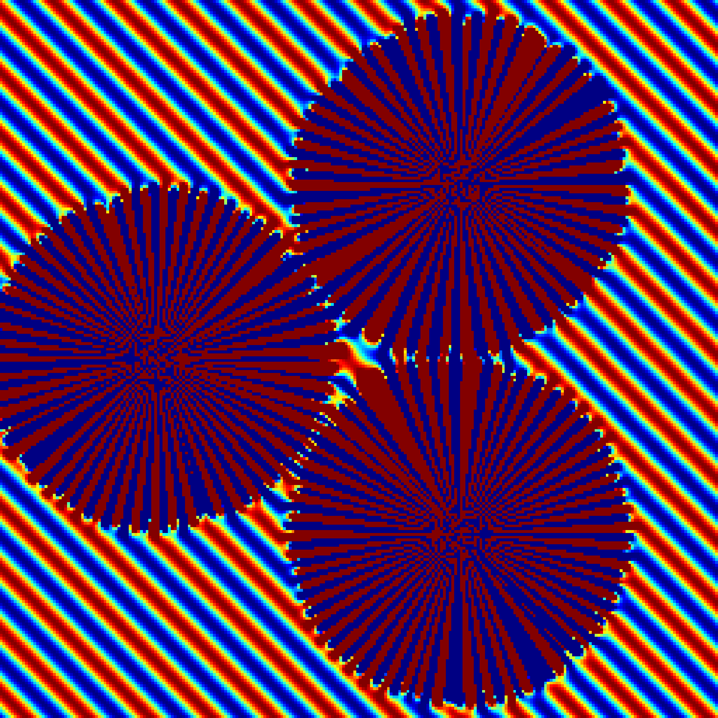
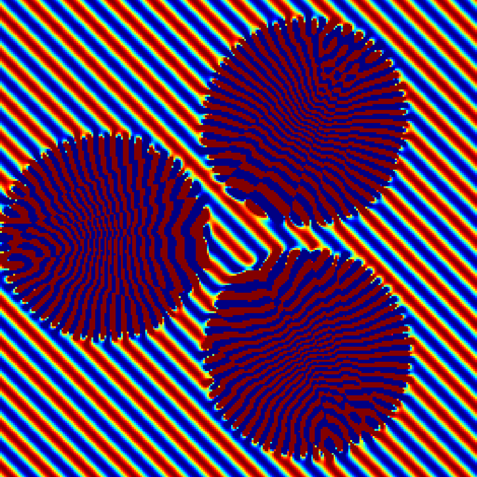
$u_{tot}$ (inactive)

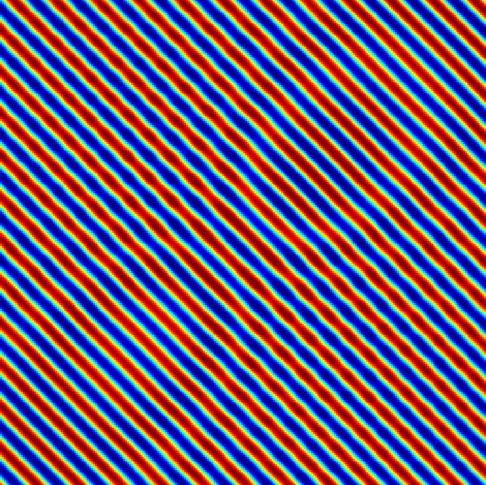
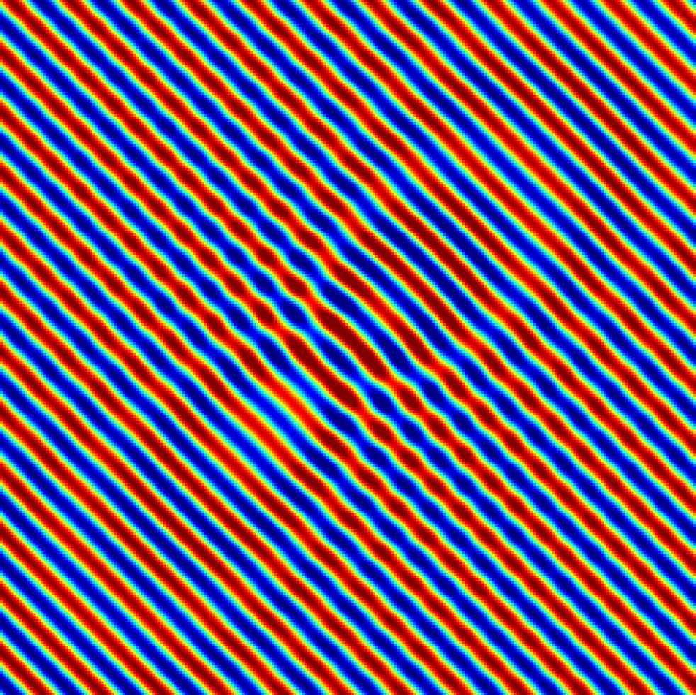
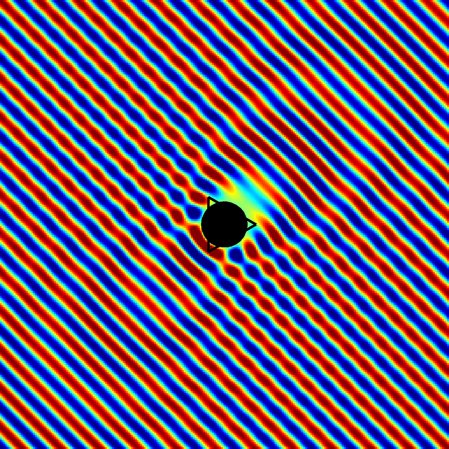
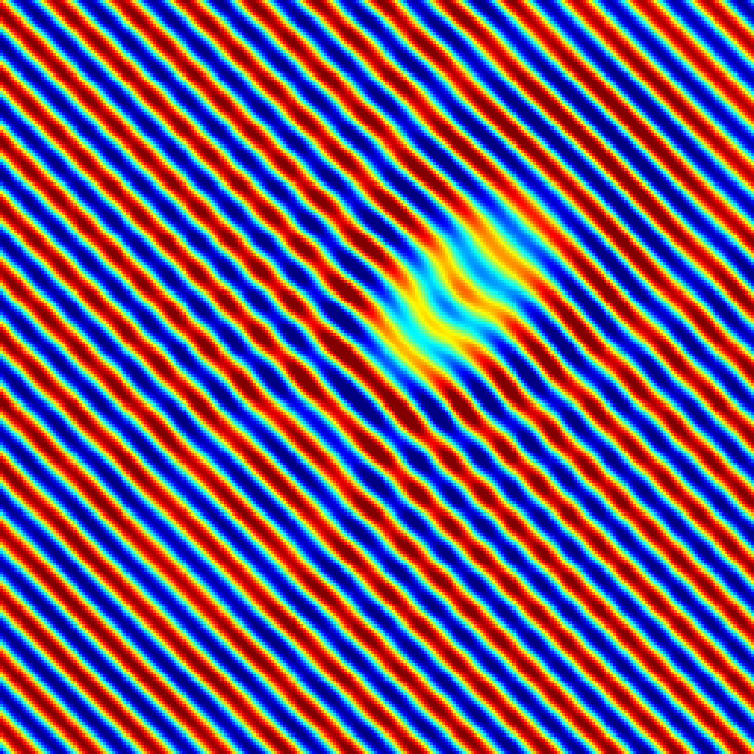
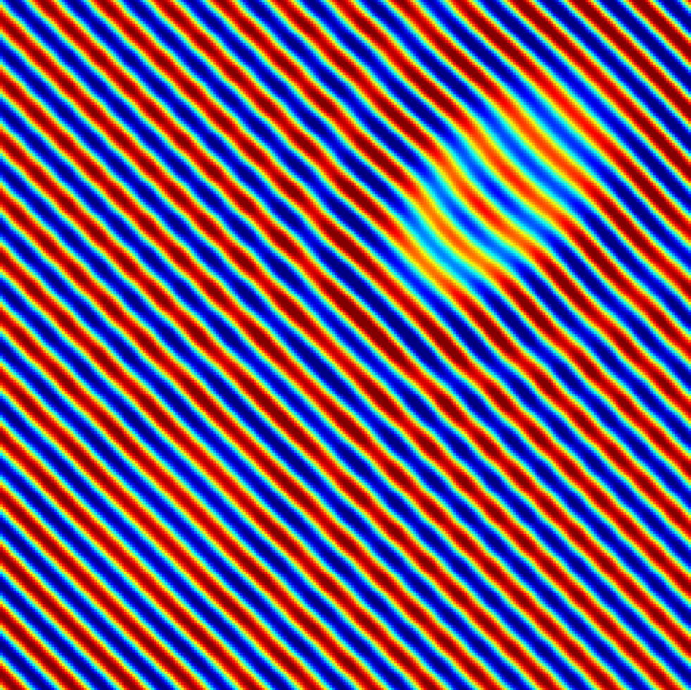
Figure 7: Constant $z$ slices of the real part of different fields, for the optimal case $\delta=3\sigma$ and with $\delta=6\lambda$. The first row shows the device field $u_{d}$ which is close to zero far from the devices and close to $-u_{i}$ in a small region close to the origin. The second and third rows show the total field when the devices are active and inactive in the presence of a scatterer. The scatterer is a sound-soft ball centered at the origin and of radius $3r_{\text{eff}}^{*}(\delta)$. Even though this ball is not completely contained inside the tetrahedron $D$, the scattered field is greatly suppressed when the devices are active, making the ball harder to detect far from the devices. The color scale is linear from -1 (dark blue) to 1 (dark red) and each box is $10\lambda\times 10\lambda$, with the $z-$axis at the center.

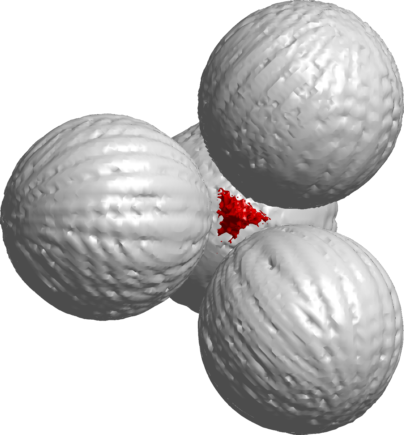
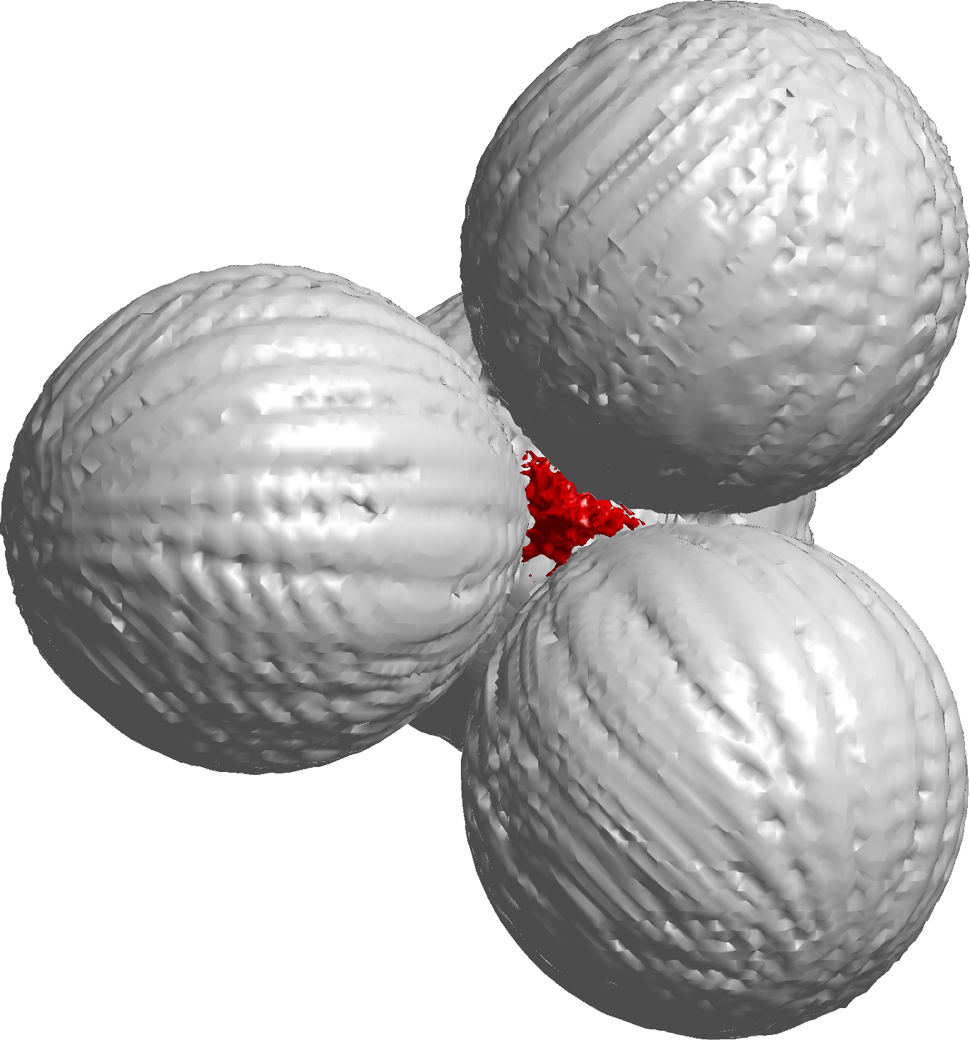
(a) $|u_{d}|=100$	(b) $|u_{d}|=5$

Figure 8: Contours of $|u_{d}|$ (gray) and $|u_{d}+u_{i}|=10^{-2}$ (red). Here the vector $(0,0,1)$ is perpendicular to plane of the page. By Green’s identity it is possible to replace the large fields inside the gray surfaces by a single and double layer potential at the gray surfaces. These “extended devices” need only to generate fields that are at most the fields on the contours that we plot and they cloak the red region without completely surrounding it.

$\delta=6\lambda$	$\delta=12\lambda$
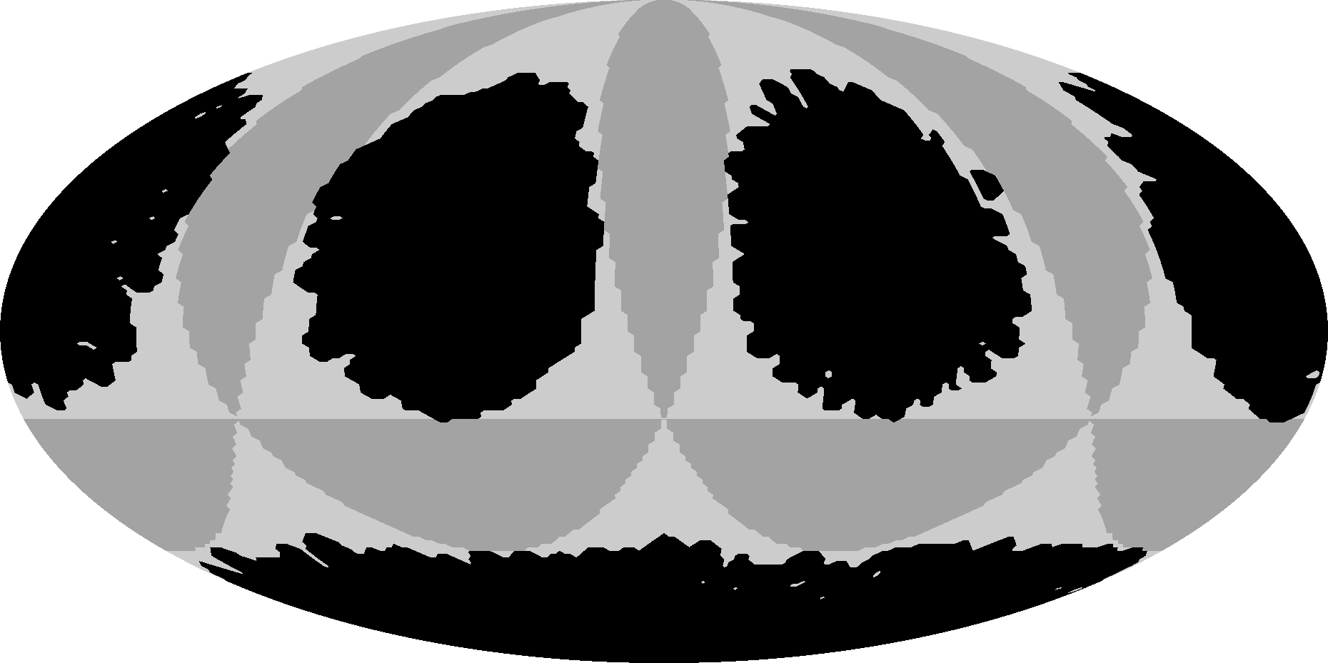
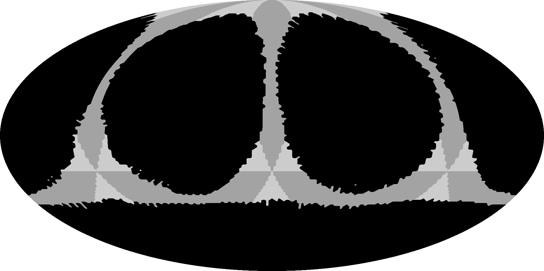
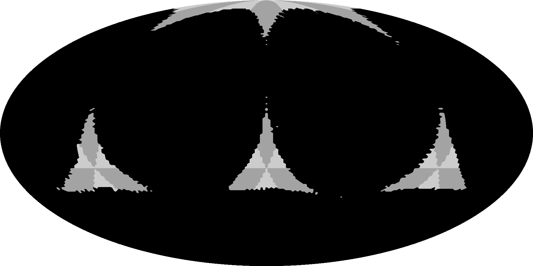
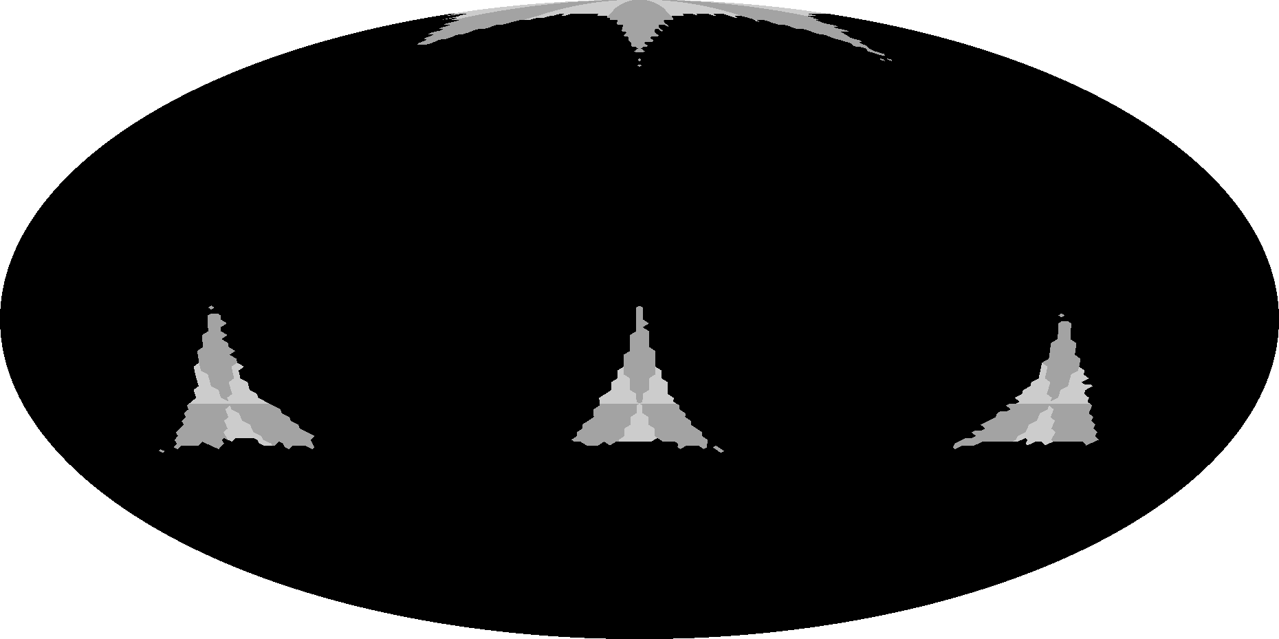
$\delta=18\lambda$	$\delta=24\lambda$

Figure 9: Cross-section of level set $|u_{d}|\geq 10^{2}$ (black) and of the region $A$ (shades of gray) on the sphere $|{\bf x}|=\sigma$ for the optimal $\sigma=\delta/3$. Here we used the equal area Mollweide projection (see e.g. Feeman (2002)). In the optimal case, each triplet out of the four balls forming $A$ meets at a single point which is a vertex of the tetrahedron $D$. Note that for the cases in the first row there are four distinct extended devices. The leftmost and rightmost spots correspond to one single device split in two by the projection.

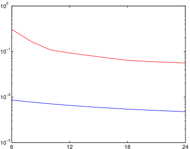
(percent)	(percent)
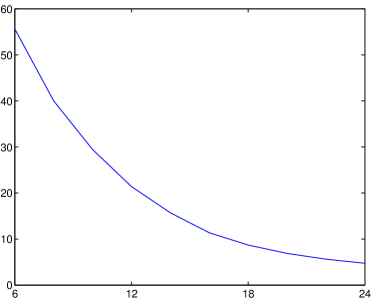
(a: $\delta/\lambda$)	(b: $\delta/\lambda$)

Figure 10: (a) Cloak performance. In red: $\|u_{i}+u_{d}\|/\|u_{i}\|$, where the norm is the $L^{2}(S(0,r_{\text{eff}}^{*}(\delta))$ norm, which measures how well we approximate the incident field inside the cloaked region. In blue: $\|u_{d}\|/\|u_{i}\|$, where the norm is the $L^{2}(S(0,2\delta))$ norm, which measures how small is the device field far away from the devices. (b) Percentage of the area outside the cross-section of the extended devices on the sphere $S(0,\sigma=\delta/3)$ for different values of $\delta$.