Intermittence of the Map of Kinetic Sunyaev-Zel’dovich Effect and Turbulence of IGM

Abstract

We investigate the possibility of detecting the turbulent state of the IGM with the kinetic Sunyaev-Zel’dovich (kSZ) effect. Being sensitive to the divergence-free component of the momentum field of the IGM, the kSZ effect might be used to probe the vorticity of the turbulent IGM. With cosmological hydrodynamical simulation in the concordance $\Lambda$CDM universe, we find that the structure functions of 2D kSZ maps show strong intermittence, and the intermittent exponents follow a law similar to the She-Leveque scaling formula of fully developed turbulence. We also find that the intermittence is weak in the maps of thermal Sunyaev-Zel’dovich (tSZ) effect. Nevertheless, the superposition of the kSZ and tSZ effects still contain significant intermittence. We conclude that the turbulent behavior of the IGM may be revealed by the observation of SZ effect on angular scales equal to or less than 0.5 arcminute, corresponding to the multipole parameter $l\geq 2\times 10^{4}$.

1 Introduction

The nonlinearly evolved cosmic baryon fluid is probably in the state of fully developed turbulence in the scale free range. With hydrodynamical simulation in the concordance $\Lambda$CDM model, the scaling exponents of the velocity structure functions of the intergalactic medium(IGM) are found to follow the She-Leveque scaling law(She & Leveque 1994) from $\sim 10h^{-1}$Mpc down to the dissipation scale (He et al. 2006; Fang & Zhu, 2011). The density field of the IGM is in good agreement with the log-Poisson hierarchy model(Liu & Fang 2008), which characterizes the statistical features of fully developed turbulence (Dubrulle 1994; She & Waymire 1995; Benzi et al. 1996). The intermittent behavior of the transmitted flux of moderate and high redshifts QSO’s Ly$\alpha$ absorption can also be well explained with the log-Poisson hierarchy cascade (Lu et al. 2009,2010).

Recently, it is further found that the IGM flow is not potential, but consists of vorticity, $\omega=\nabla\times{\bf v}$, on scales from hundreds kpc to a few Mpc at $z\sim 0$(Zhu et al. 2010). The power spectra of the vorticity field $P_{\omega}(k)$ and the velocity field $P_{v}$ satisfy the relation $P_{\omega}(k)=k^{2}P_{v}(k)$ on scales from $0.2$ to about $3h^{-1}$ Mpc, indicating that the velocity field of the IGM is dominated by vorticity on this scale range.

These results motivate us to study the imprints of the turbulent IGM in the kinetic Sunyaev-Zel’dovich (kSZ) effect. The kSZ effect is the CMB temperature fluctuations due to the scattering of CMB photon by the bulk motion of free electrons in the IGM with radial peculiar velocity field ${\bf v}(t,{\bf r})$ (Sunyaev & Zel’dovich 1972,1980). It can be given by an integral along a line of sight $s$ as

$$\Delta T(\hat{\bf n})/T=b(\hat{\bf n})=-\int\sigma_{T}\left(\frac{n_{e}{\bf v}\cdot\hat{\bf n}}{c}\right)ds$$ (1)

where $\sigma_{T}$ is the Thompson scattering cross section. The quantity $n_{e}$ is the number density of electrons, and ${\bf n}$ is the unit vector in the direction of the line of sight. It has been pointed out that the kSZ effect is largely contributed by the divergence-free component of the momentum density field $n_{e}{\bf v}$. The kSZ effect would grow fast when the velocity field transits from a gradient, or curl-free field to curl-dominant one (Vishiniac 1987; Ma et al. 2002; Zhang et al 2004). In other words, the kSZ effect is sensitive to the vorticity of the IGM velocity field.

Many studies on the kSZ effect have been done with semi-analytical method or hydrodynamical simulation (e.g. Springel et al. 2001; da Silva et al. 2001; Zhang et al. 2002, 2004; Roncarelli et al. 2007; Atrio-Barandela et al 2006, 2008; Cunnama et al 2009). Most of these works mainly focused on the one-point probability density function distributions, the power spectrum, and their difference with the corresponding results of the tSZ effect. The tSZ effect, usually in terms of $y({\bf n})$, is calculated by a line integral of the pressure of the IGM (Sunyaev & Zeldovich, 1980). In this letter, we use structure functions to extract the non-Gaussian features of two-dimensional kSZ and tSZ maps composed from hydrodynamical simulation in the $\Lambda$CDM framework. We find that the kSZ maps are highly intermittent, and the intermittent exponents are consistent with model of fully developed turbulence. While for the tSZ maps the intermittence is relatively weak. For the maps given by the superposition of the kSZ and tSZ effects, the intermittent features are still significant on angular scale $l\sim 2\times 10^{4}$. The kSZ effect provides a useful tool to probe the turbulent state of the IGM.

2 Map making and power spectrum

1. Cosmological simulation and map making. We perform our cosmological simulation using the WIGEON code (Feng et al. 2004), which is a hybrid cosmological hydrodynamic/N-body code based on weighted essentially non-oscillatory (WENO) method. It has been used to study the tSZ effect(Cao et al. 2007), Ly$\alpha$ forests (Lu et al 2009, 2010), the vorticity of the IGM (Zhu et al 2010) and the effect of IGM turbulence on the baryon fraction (Zhu et al. 2011). The simulation is evolved from $z=99$ to $z=0$ in a periodic box of side length 25 $h^{-1}$ Mpc with a $512^{3}$ grid and an equal number of dark matter particles. The box size 25 $h^{-1}$ Mpc is reasonable, as it is much larger than the typical scales of vortices. To test the convergence, we also run a comparison simulation in a larger box of 100 $h^{-1}$ Mpc with the number of grid and particles remain $512^{3}$. The cosmological parameters adopted here are $(\Omega_{m},\Omega_{\Lambda},h,\sigma_{8},\Omega_{b},n_{s})=(0.274,0.726,0.705,0.812,0.0456,0.96)$ (Komatsu et al., 2009). Radiative cooling and heating are the same as Theuns et al. (1998) with a primordial composition of $X=0.76,Y=0.24$, and star formation and its feedback are not included.

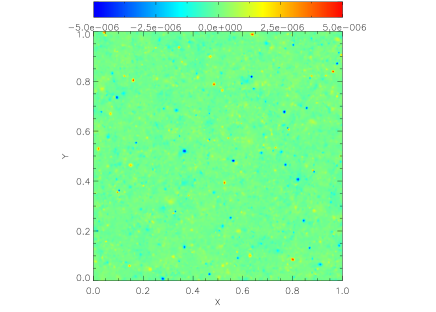
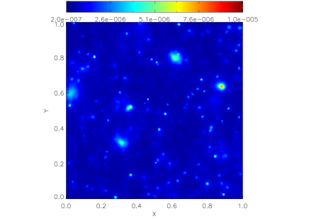
Figure 1: Maps of the kSZ effect (left) and the tSZ effect(right),showing the $b$, $y$ parameter in a $15^{\prime}\times 15^{\prime}$ patch, respectively.

We produce two-dimensional maps of the kSZ and tSZ effects using a conventional method, e.g., refer to Gnedin & Jaffe(2001), or Zhang et al(2002). During the cosmological simulation, two-dimensional projections of the kSZ and tSZ effects through the whole simulation box along the x-, y- and z-directions are stored as sectional maps at different redshifts since $z=6$, as both the kSZ and tSZ effects are dominated by contributions from $z=6$ to $z=0$(Roncarelli et al. 2007). The redshift intervals between the successive outputs are given by the light-crossing time through the box. We have 240 and 60 outputs for the 25 $h^{-1}$ Mpc and 100 $h^{-1}$ Mpc simulation run respectively. We then stack sectional maps, one at each outstored redshift, to make a single kSZ or tSZ map. Each sectional map is randomly selected from one of the three box projections along different axes direction at the corresponding redshift. To reduce the artificial replication effect in the simulated periodic universe (Gnedin & Jaffe 2001), we randomly place the center of the selected 2-D sectional map, and then rotate and flip it around any of the six box edge. We compose $50$ maps of the kSZ and tSZ effects respectively in size of $15^{\prime}$ on a side, corresponding to the angle the box extended at z=6, with pixel resolution $512\times 512$, and $1024\times 1024$ for the 25 $h^{-1}$ Mpc run. We also produce 50 maps of the kSZ and tSZ effects in size of $1^{\circ}$ respectively with pixel resolution $1024\times 1024$ for the 100 $h^{-1}$ Mpc run. Figure 1 demonstrates an example of the kSZ and tSZ maps obtained from the 25 $h^{-1}$ Mpc run. Although the kSZ effect is smaller than the tSZ effect in magnitude at center region of dense halos, it is comparable to, and even larger than the tSZ effect in their outskirts.

2. Power spectrum. The power spectra of the kSZ(b) and tSZ(y) effects are shown in the left panel of Figure 2, which are obtained by averaging over 50 maps of the 25 $h^{-1}$ Mpc run respectively under the small-angle approximation. The power spectrum of the kSZ effect grows rapidly when the multipole parameter $l>10^{4}$, and exceeds the tSZ power spectrum at around $l\sim 2\times 10^{4}$, corresponding to the angular scales $\leq 0^{\prime}.5$. This behavior is basically consistent with result given by the lognormal model of the IGM (Astro-Barandela et al. 2008) and similar to those in Zhang et al.(2004) and Roncarelli et al.(2007). We also present the power spectrum of the kSZ and tSZ maps integrated from $z=6$ to 4, 2, and 1 in Fig. 2. It shows that the kSZ power spectrum is mostly contributed by the electron motion in the redshift range of $z\sim 1-2$. This redshift dependence can be interpreted in term of the development history of the IGM turbulence in the expanding universe recognized recently by Zhu et al. (2010). Turbulence and vorticity, i.e., the curl part of velocity, in the IGM remains weak till $z\sim 4$, and thereby the level of the power spectrum of the kSZ effect would be low at $z>4$. After $z\sim 1$, both the covered scale range and intensity of turbulence and vorticity will grow continuously. However, the number density of electrons $n_{e}$ in the outskirts of collapsed halos decreases with the cosmic expansion, the integrated kSZ effect gains most of its weight in the redshift range $z\sim 2-1$. In the same redshift range, the velocity field of IGM is in the state of fully developed turbulence between $0.2h^{-1}$ Mpc and $0.8h^{-1}$ Mpc, corresponding to the angle scale range of $0^{\prime}.2-1^{\prime}.0$, i.e.,$10^{4}<l<5\times 10^{4}$, within which the peak of the kSZ power spectrum appears.

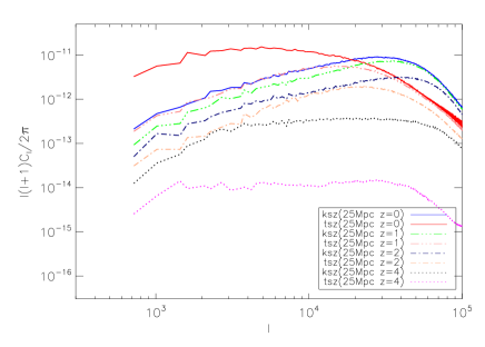
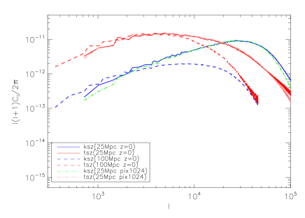
Figure 2: Left: the power spectrum of the kSZ (solid blue) and tSZ (solid red) effects integrated from $z=6$ to 0 and averaged over 50 samples produced by 25$h^{-1}$ simulation with pixel resolution $512^{2}$; also the results that integrated from $z=6$ to $z=4$, 2, 1 are shown .Right: Comparison to the power spectrum integrated from $z=6$ to $z=0$ for samples of 25 $h^{-1}$ Mpc simulation with pixel resolution $1024\times 1024$(dash), and 100 $h^{-1}$ Mpc simulation with pixel resolution $1024\times 1024$ (dash dotted).

To check the numerical convergence, we compare the power spectrum of the kSZ and tSZ effects generated with different pixel resolutions or simulation box size in the right panel of Figure 2. Obviously, once the simulation resolution is given, the resolution of SZ maps has a small impact on the result. The 25 $h^{-1}$ Mpc run may underestimate the power spectrum of the kSZ and tSZ effects due to the lack of large scale perturbations. However, we find that this effect is mildly weak on scales $l\geq 10^{3}$ . Although the lack of perturbations large than the box size may affect the power spectrum on scales $l<10^{3}$, the primary temperature fluctuations will dominate over the tSZ and kSZ effects(Springel et al. 2001; Zhang et al. 2004; Roncarelliet al. 2007). The statistical features in that scale range are out the scope of this letter. On the side of small scales, $l\geq 10^{4}$, the power spectrum of the 100 $h^{-1}$Mpc simulation run falls rapidly, and is significantly lower than the 25 $h^{-1}$Mpc run. This feature has been addressed in previous works (Gnedin & Jaffe 2001; Zhang et al. 2004), which should result from the poor resolution of the 100 $h^{-1}$Mpc simulation.

3 Intermittence of the tSZ and tSZ maps

1. Structure functions. To identify the intermittence of the kSZ maps, we use the dimensionless structure functions defined by

$$S_{p}(\theta)=\frac{\langle(\delta b_{\theta})^{p}\rangle}{\langle(\delta b_{\theta})^{2}\rangle^{p/2}},$$ (2)

where $b_{\theta}\equiv b(\hat{\bf n})-b(\hat{\bf n^{\prime}})$. $\theta$ is the angle between two directions $\hat{\bf n}$ and $\hat{\bf n^{\prime}}$. For a Gaussian field, $S_{p}(\theta)$ is independent of $\theta$ and equals to $(p-1)!!$, here $p$ is even integer (Pando et al 2002). The structure functions of the tSZ maps can be calculated by replacing $b(\hat{\bf n})$ with $y(\hat{\bf n})$ in eq(2).

The intermittence of the velocity field ${\bf v}$ in fully developed turbulence is characterized by $\langle(\delta v_{r})^{p}\rangle\sim r^{\zeta(p)}$, where the intermittent exponents $\zeta(p)$ are given by the SL scaling law(She & Leveque 1994, She et al. 2001). If the kSZ maps contains signatures of the intermittence caused by the fully developed turbulence in the IGM, the structure functions should follow a power law

$$S_{p}(\theta)\propto\theta^{-\xi(p)}.$$ (3)

According to the SL scaling law, the intermittent exponents are given by

$$\xi(p)=(p/2)\zeta(2)-\zeta(p)=\alpha(1+\beta)[p-2(1-\beta^{p})/(1-\beta^{2})],$$ (4)

where $\alpha$ and $\beta$ are free parameters, and $\xi(2)=0$. The non-Gaussianity is typically measured by parameter $\beta$ (Liu & Fang 2008). In a Gaussian field, $\beta=1$, while in a intermittent field $\beta<1$. The basic features of the intermittent exponents $\xi(p)$ are 1.) when $p$ is small, $\xi(p)$ is a nonlinear function of $p$, and has $d^{2}\xi(p)/dp^{2}>0$; 2.) when $p$ is large, $\xi(p)$ has to be a straight line with slope $\alpha(1+\beta)$ as $\beta<1$;

The non-Gaussianity of the kSZ maps is affected by two major factors. First, the kSZ effect is given by an integral of the momentum density of the electrons, $n_{e}{\bf v}$ along the line of sight. The non-Gaussian behavior of $n_{e}{\bf v}$ will be developed significantly by intermittence either in the velocity field ${\bf v}$ or the electrons density field $n_{e}$. If both of these two fields are intermittent, the multiplication will lead to enhancement of the non-Gaussianity in the momentum density field. Second, the maps of $b({\bf n})$ are given by the summation of the momentum field $n_{e}{\bf v}$ in successive redshifts intervals, therefore the non-Gaussianity might be reduced according to the central limit theorem. However, the statistical behaviors governed by the central limit theorem will be remarkably retarded by the development history of the IGM turbulence. As mentioned in §2, the integrated kSZ effect will be dominated by such turbulent flows fully developed in the range $z\sim 1-2$. Moreover, for intermittent fields in which large deviation events always occur, the central limit theorem acts slowly (Jamkhedkar et al 2003, Fujisaka & Inoue 1987; Frisch 1996). In theory, the kSZ maps generated by eq.(1) may still contain the signatures of the non-Gaussian statistical properties of turbulence. The case with the tSZ effect is different as its non-Gaussianity is mainly given by the electrons’ density and temperature field.

3. Intermittent exponents. Figure 3 presents the structure functions of the kSZ maps in the angular range $0^{\prime}.05-1^{\prime}.5$. As a comparison, we also plot the structure functions of the tSZ and total SZ effects, the latter is the superposition of the kSZ and tSZ effects.

A remarkable feature displayed in Figure 3 is that the structure functions of the kSZ, tSZ and total SZ maps are in agreement with the power law in eq.(3). It indicates that all the maps are essentially non-Gaussian. In addition, the correlation between $\ln S_{p}(\theta)$ and $\ln\theta$ of the kSZ effect is much stronger than that of the tSZ effect, suggesting that the non-Gaussianity of the kSZ maps is much significant.

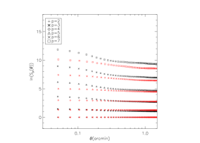
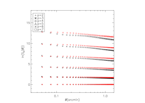
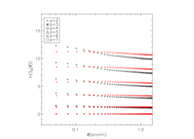
Figure 3: $\log S_{p}(\theta)$ vs. $\theta$ of the maps of the kSZ (left), tSZ (middle) and total SZ (kSZ + tSZ) (right) effects. They are averaged over 50 samples. Black and red curves represent the samples of 25 $h^{-1}$ and 100 $h^{-1}$ Mpc respectively.

Figure 3 shows that on scales $\theta>0.5$ arcmins the logarithmic structure function $\log S_{p}(\theta)$ of the kSZ effect obtained in the 25 $h^{-1}$ and 100 $h^{-1}$ Mpc simulations remain the same till $p=5$, and the deviations on 6th and 7th orders are visible, but still less than 10%. On small scales $\theta<0.5$ arcmins, the logarithmic structure functions of the kSZ effect in the 100 $h^{-1}$ Mpc run are clearly lower than the 25 $h^{-1}$ Mpc run. However, for the tSZ effect, we do not see any significant difference between these two simulations in overall angular range $0^{\prime}.05-1^{\prime}.5$. This feature is most likely caused by the velocity field having stronger dependence on the simulation resolution than the temperature field, which has been actually recognized by the power spectrum comparison. It indicates that the kSZ is more sensitive to the non-Gaussianity of the turbulence, namely, the non-Gaussianity of the total SZ maps should be largely attributed to the kSZ effect.

The intermittent exponents $\xi(p)$ as a function of the order $p$ are plotted in Figure 4. For the samples produced in the 25 $h^{-1}$ Mpc simulation, the intermittent exponents $\xi(p)$ display a tight linear relation with the order parameter $p$ in the kSZ maps, but is relatively weak for the tSZ maps. The intermittent exponents $\xi(p)$ can be best fitted as a function of $p$ by eq.(4) with $\alpha=0.18,\ \beta=0.25$, $\alpha=0.08,\ \beta=0.7$ and $\alpha=0.11,\ \beta=0.41$ for the kSZ, tSZ and total SZ effects, respectively.

In comparison, the right panel of Figure 4 presents the intermittent exponents $\xi(p)$ measured in the 100 $h^{-1}$ Mpc simulation. Clearly, they have a weaker dependence on $p$. The least-square fitting gives $\beta=0.85$, $\beta=0.95$ and $\beta=0.92$ for the kSZ, tSZ and total SZ effects respectively. It implies that, the non-Gaussianity characterized by the parameter $\beta$ of samples produced by 100 $h^{-1}$ Mpc simulation is much weaker than the 25 $h^{-1}$ Mpc simulation. It can be concluded that the nonlinear development of the velocity field at small scales can produce stronger non-Gaussianity.

Figure 4: The intermittent exponents of the maps of kSZ, tSZ and (kSZ+tSZ) in 25 Mpc(left) and 100 Mpc(right) simulation box.

4 Discussions and Conclusions

With cosmological hydrodynamical simulation in the concordance $\Lambda$CDM model, the turbulent cosmic baryon fluid is found to yield intermittence in the second order CMB temperature fluctuation due to the kSZ effect, which can be described in term of the structure functions. The structure functions can be applied to identify the types of the non-Gaussianity (Pando et al 2002). We demonstrate that the structure functions of the kSZ maps possess the typical behavior of fully developed turbulence, i.e. the intermittent exponents follow a law similar to the She-Leveque universal scaling. Although the weakly intermittent tSZ effect will be dominant over the kSZ effect in the center regions of virialized halos, the total SZ effect still displays significant intermittence. Therefore, it is expected that the intermittence of the kSZ effect would remain detectable on angular scales $0^{\prime}.05\sim 1^{\prime}.0$ in noisy maps, if the noises from foreground and others sources are not stronger than the tSZ effect.

Star formation and its feedback on the IGM has not been included in the simulation. Even though the SZ effect is strong in massive collapsed objects with hot gas, the intermittent exponents would not be dominated by the hot collapsed objects, because $S_{p}$ is given by the ratio of the fluctuations of the SZ effect [eq.(2)]. Accordingly, it is concluded that the turbulent behavior of the IGM may be detectable by high quality observation of CMB temperature fluctuations on angular scales $\leq 1^{\prime}.0$, i.e., the multipole parameters $l\geq 2\times 10^{4}$, which, however, is below the detection limit of current observational projects.

References

- (1)
- (2) Atro-Barandela, & F., Mücket, 2006, ApJ, 643, 1
- (3)
- (4) Atro-Barandela, F., Mücket, & G’enova-Santos, 2008, ApJ, 674, L61
- (5)
- (6) Benzi, R., Biferale, L. & Trovatore, E., 1996, Phys. Rev. Lett. 77, 3114
- (7)
- (8) Bi, H. G., Boerner, G., & Chu, Y., 1992, A&A, 266, 1
- (9)
- (10) Cao, L., Liu, J.R. & Fang, L.Z. 2007, ApJ, 661, 641
- (11)
- (12) Cunnama, D., Faltenbacher, A., Cress, C. & Passmoor, S. 2009, MNRAS, 397, L41
- (13)
- (14) da Silva, A. C., Barbosa D., Liddle A. R., & Thomas P. A., 2001, MNRAS, 326, 155
- (15)
- (16) Dubrulle, B. 1994, Phys. Rev. Lett. 73, 959
- (17)
- (18) Fang, L. Z., Bi, H. G., Xiang, S.P., & Boerner, G., 1993, ApJ, 413, 477
- (19)
- (20) Fang, L. Z. & Zhu, W.S., 2011, Advances in Astronomy, 2011, Artcle ID 492480
- (21)
- (22) Frisch, U. 1996, Turbulence, (Cambridge Press)
- (23)
- (24) Fujisaka, H., & Inoue, M., 1987, Prog. Theor. Phys. 77, 1334
- (25)
- (26) Gnedin N. Y., Jaffe A., 2001, ApJ, 551, 3
- (27)
- (28) He, P., Liu, J., Feng, L.L., Shu, C.-W., & Fang, L.Z. 2006, Phys. Rev. Lett, 96, 051302
- (29)
- (30) Jamkhedkar, P., Feng, L.L., Zhange, W., Kirkman, D. Tytler, D. & Fang, L.Z. 2003, MNRAS, 343, 1110
- (31)
- (32) Komatsu, E., et al. 2009, ApJS, 180, 330
- (33)
- (34) Liu, J.R., & Fang, L.Z. 2008, ApJ, 672, 11
- (35)
- (36) Lu, Y., Chu, Y.Q., & Fang, L.Z. 2009, ApJ, 691, 43
- (37)
- (38) Lu, Y., Zhu, W.S., Chu, Y.Q., Feng, L.L. & Fang, L.Z. 2010, MNRAS, 408, 452
- (39)
- (40) Ma, C. P., & Fry, J. N., 2002, Phys. Rev. Lett, 88, 211301
- (41)
- (42) Pando, J., Feng, L.L., Jamkhedkar, P., Zheng, W., Kirkman, D., Tytler, D. and Fang, L.Z. 2002 ApJ, 574, 575
- (43)
- (44) Roncarelli, M., Moscardini, L., Borgani, S., & Dolag, K., 2007, MNRAS, 378, 1259
- (45)
- (46) She, Z.S., & Leveque, E. 1994, Phys. Rev. Lett. , 72, 336
- (47)
- (48) She, Z.S. & Waymire, E.C., 1995, Phys. Rev. Lett. 74, 262
- (49)
- (50) She, Z. S., Ren, K., Lewis, G. S., & Swinney, H. L., 2001, Phys. Rev. E, 64, 016308
- (51)
- (52) Springel, V., White, M. & Hernquist, L., 2001, ApJ, 549, 681
- (53)
- (54) Vishiniac, E.T. 1987, ApJ, 322, 597
- (55)
- (56) Sunyaev, R., & Zeldovich, Y.B., 1972, Commun. Astrophys. Space Phys., 4, 173
- (57)
- (58) Sunyaev, R., & Zeldovich, Y.B., 1980, ARA&A, 18, 537
- (59)
- (60) Theuns, T., Leonard, A., Efstathiou, G. ,Pearce, F. R., & Thomas, P. A. 1998, MNRAS, 301, 478
- (61)
- (62) Zhang, P.J., Pen, U. L., & Wang, B., 2002, ApJ, 577, 555
- (63)
- (64) Zhang, P.J., Pen, U.-L., & Trac, H. 2004, MNRAS, 347, 1224
- (65)
- (66) Zhu, W. S., Feng, L. L., & Fang, L. Z., 2010, ApJ, 712, 1
- (67)
- (68) Zhu, W. S., Feng, L. L., & Fang, L. Z., 2011, MNRAS, in press, arXiv:1103.1058