Fano effect and nonuniversal phase lapses in mesoscopic regime of transport

Abstract

The transmission probability and phase through a few-electron quantum dot are studied within a resonance theory for the strong coupling regime to the conducting leads. We find that the interaction between overlapping resonances leads to their separation in the complex energy plane and to the decoherent dephasing of the resonant modes. The appearance of the Fano effect is conditioned not only by the induced dephasing generally associated with a phase lapse, but also by a favorable parity of the resonant modes. To identify the contribution of each resonance to the transmission, we propose, in the case of overlapping resonances, a decomposition of the scattering matrix in resonant terms and a background. The resonant contributions are approximated by Fano lines with complex asymmetry parameters and the background by a constant. The conductance and the transmission phase calculated within this approach reproduce the generic features of the experimental data.

I Introduction

The Fano effectFano (1961); Fano and Rau (1986); Miroshnichenko et al. (2010), responsible for the asymmetric peaks in the absorption or transmission spectra through quantum systems, is nowadays one of the most studied phenomena. This effect was experimentally observed for a large variety of quantum systems, in the neutron scatteringAdair et al. (1949), atomic photoionizationFano (1961); Fano and Rau (1986), Raman scatteringCedeira et al. (1973), optical absorptionFaist et al. (1997) and, recently, in transport through semiconductor quantum dotsGöres et al. (2000); Kobayashi et al. (2002, 2003). The universal presence of the Fano effect attests the fact that it directly follows from the principles of the quantum mechanics. According to these principles, the measurements done on a quantum system necessarily perturb it. There exists a coupling between the quantum system and environment and this coupling causes an indirect transfer, i.e. by dint of a continuum of states, between two eigenstates of the system. This process accompanies the direct transition between states and the two pathways - the direct and the indirect ones - interfere. This is essentially the mechanism that undergoes the Fano effect. In a recent studyKroner et al. (2008) even the nonlinear Fano effect has been observed in experiments done on semiconductor quantum dots. In the nonlinear regime, the direct transition between two eigenstates of the quantum system saturates and, after that, in the presence of a continuum of states, the indirect transitions become more and more important leading to a pronounced asymmetry of the line shape in the absorption cross-section.

The notable technological progress in the last decade has enabled the experimental observation of the Fano effect in mesoscopic systems and an interesting domain for the theoretical studies has been opened. There are two categories of experiments dedicated to this issue. The first one was proposed by Göres et al.Göres et al. (2000) in 2000. A quantum dot strongly coupled to the contacts was defined, by means of top gates, in a two dimensional electron gas (2DEG) and broad and asymmetric profiles were observed in conductance. They are the signature of the Fano effect but in this case one can not define two spatially separated interfering pathways. The complex asymmetry parameter necessary for fitting the experimental data reflects the open character of the system, i.e. a quantum system without time reversal symmetryO.Entin-Wohlman et al. (2002). In 2002 Kobayashi et al.Kobayashi et al. (2002) have proposed a system in which the two interfering pathways are spatially separated. A quantum dot with well separated energy levels is placed in one arm of an Aharonov-Bohm ring and the other arm is unperturbed. The electrons travel from the source to the drain contact along the two pathways and the line shapes of the transmission peaks become broad and asymmetricKobayashi et al. (2002, 2003); Nakanishi et al. (2004), certifying the presence of the Fano effect. These two experiments were followed by many experimentalKobayashi et al. (2002, 2003, 2004); Sato et al. (2005); Avinun-Kalish et al. (2005); Kroner et al. (2008) and theoreticalNöckel and Stone (1994, 1995); Clerk et al. (2001); Racec and Wulf (2001); Racec et al. (2002); O.Entin-Wohlman et al. (2002); Magunov et al. (2003); Nakanishi et al. (2004); Johnson et al. (2004); Moldoveanu et al. (2005); Satanin and Joe (2005); Mendoza et al. (2008) studies dedicated to the Fano effect in mesoscopic systems.

For understanding the interference process in mesoscopic systems some considerations about the transport mechanism through these systems are needed. In transmission experiments an electron is transfered from a state at the Fermi energy in the source contact to a state at the Fermi energy in the drain contact through a quantum system, usually a quantum dot. If the quantum system is separated from the contacts by high barriers the electron has a nonzero probability to tunnel the barriers and reaches the drain contact. This probability is significant if an energy level of the quantum system matches the Fermi energy. In this case a resonant tunneling takes place and the total transmission shows a thin and quasi-symmetric maximum, i.e. a Coulomb blockade peakK.Ferry et al. (2009). If the confinement barriers are lowered, the energy levels of the quantum dot become broad. As long as they do not overlap the mechanism described above works further. The transmission peaks become also broad and slight asymmetricRacec and Wulf (2001) and their widths correspond to the width of the resonances supported by the open quantum system. The asymmetry of the Fano profile in transmission has at the origin the existence of many resonances; A narrow resonance with the real energy around the Fermi energy intermediates the direct electron transfer through the quantum system, while the other resonances define indirect pathways that lead to interference and, consequently, to the Fano effectRacec et al. (2010). To increase further the asymmetry of the Fano profile and therefore to amplify the Fano effect in nanostructures, one needs overlapping resonances. They are supported by scattering potentials that couple the conducting channels due to their nonseparable character. In Ref. Racec et al., 2010 we showed that the channel mixing yields pairs of resonances very close in energy, but with different widths. They are ideal for interference and are responsible for strong asymmetric peaks and dips in conductance through a quantum dot. A competing process that increases the separation of the resonance energies is the Coulomb interaction. In Ref. Karrasch et al., 2007a is reported that the renormalization effects induced by the local Coulomb interaction lead to narrow and broad resonant levels that overlap. Each time a narrow level crosses the Fermi energy and the broad level, a Fano-type antiresonance accompanied by a phase lapse occursKarrasch et al. (2007b). Thus, not only the line shape of the transmission probability through quantum systems is a fingerprint of the Fano effect, but also the phase evolution.

For a systematic analysis of the Fano effect in open quantum systems, we investigate in this paper a quantum dot strongly coupled to the conducting leads via quantum point contacts and compute the transmission probabilities and phases through the system. Similar to the effective one-dimensional caseRacec and Wulf (2001), the peaks and dips in the total transmission are approximated as Fano functions with a complex asymmetry parameter. Each peak and dip can be associated with a resonance or a set of overlapping resonances. In the frame of our resonance theoryRacec and Wulf (2001); Racec et al. (2010), we give a method to compute the Fano asymmetry parameters for an arbitrary potential landscape within the quantum system. Based on the discussion in Ref. Oreg, 2007, we analyze further the relation between the asymmetry parameter and the phase evolution of the electrons transfered to the quantum dot. The phase of the transmission probability through open quantum dots is still an open problem in the mesoscopic physics, intensively studied experimentallyYacoby et al. (1995); Schuster et al. (1997); Avinun-Kalish et al. (2005); Katsumoto (2007) and theoretically Hackenbroich and Weidenmüller (1996); Oreg and Gefen (1997); Lee (1999); Levy and Büttiker (2000); Silva et al. (2002); Golosov and Gefen (2006); Karrasch et al. (2007b, a); Oreg (2007); Bertoni and Goldoni (2007); Müller and Rotter (2009); Hecht et al. (2009); Ţolea et al. (2010) in the last years. In contrast to the universal behavior, specific for high populated quantum dots, for the few-electron quantum dot studied here, we show, as expected, mesoscopic features of the transmission phases.

II The model

The transmission phenomena through weakly confined quantum dots Göres et al. (2000); Avinun-Kalish et al. (2005); Goldhaber-Gordon et al. (1998); Kobayashi et al. (2002, 2003) are still a puzzling problem because the limit of the strong coupling is quite similar to a vanishing couplingO.Entin-Wohlman et al. (2002). Trying to decode this puzzle, we have proposed in Ref. Racec et al., 2010 a model for the scattering in a nonseparable, low confining potential inside a quantum wire tailored in 2DEG. While the positions of the barriers inside the quantum wire, Fig. 1, are given by the top gates (see SEM micrograph of the device in Refs. Göres et al., 2000 and Avinun-Kalish et al., 2005), their heights are the only free parameters in our model. The two point contacts shown in Fig. 1 ensure the nonseparable character of the scattering potential.

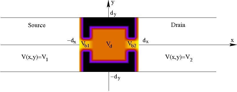
Figure 1: The geometry of a quantum dot embedded inside a quantum wire: $2d_{x}=2d_{y}=175$ nm, the barrier width is $d_{b}\simeq 35$ nm, and the point contact regions are about 35 nm $\times$ 35 nm. Potential energy $V(x,y)$ in the quantum wire (dark corresponds to high values and bright to low ones): $V_{b0}=100$ meV, $V_{b1}=V_{b2}=2.5$ meV and $V_{1}=V_{2}=0$. The potential energy felt by the electrons inside the dot is $V_{d}$. At each interface between two domains the potential energy varies linearly within a distance of 10 nm. Outside the quantum wire there is a hard wall potential. The density of 2DEG inside which the quantum dot is defined is $N_{S}=8.1\times 10^{11}$ cm^-2 and the Fermi energy is $E_{F}=29,6$ meV.

The confinement potential of the dot and especially the quantum well inside which the electrons are localized are shallow Avinun-Kalish et al. (2005). The quantum dot created in this way is quite strongly coupled to the contacts and the open character becomes dominant determining the transport properties through the quantum system. In the strong coupling regimeGöres et al. (2000); Avinun-Kalish et al. (2005); Goldhaber-Gordon et al. (1998); Kobayashi et al. (2002, 2003), the two quantum point contacts act as deep quantum wells ($V_{b1}=V_{b2}\ll V_{b0}$) in the lateral direction.

II.1 Scattering matrix

In Ref. Racec et al., 2010 we provide a description in detail of the scattering process in a 2D nonseparable potential in terms of resonances. The 2D Schrödinger equation for the localized scattering potential $V(x,y)$ is solved directly using the scattering theory and the R-matrix formalism.

The scattering functions, the most appropriate solutions of the 2D Schrödinger equation in the case of a localized scatterer, are given in terms of the generalized scattering matrix ${\mathbf{\cal{S}}}$. Outside the scattering region, i.e. the dot region, they have the expressions Racec et al. (2010)

$$\psi_{n}^{(s)}(E;x,y)=\frac{\theta[N_{s}(E)-n]}{\sqrt{2\pi}}\begin{cases}\delta_{s1}\exp{[i\;k_{1n}\;(x+d_{x})]}\;\phi_{n}(y)+\sum_{n^{\prime}=1}^{\infty}\limits\mbox{${\mathbf{\cal{S}}}$}^{T}_{sn,1n^{\prime}}(E)\exp{[-i\;k_{1n^{\prime}}\;(x+d_{x})]}\;\phi_{n^{\prime}}(y),&x\leq-d_{x}\cr\delta_{s2}\exp{[-i\;k_{2n}\;(x-d_{x})]}\;\phi_{n}(y)+\sum_{n^{\prime}=1}^{\infty}\limits\mbox{${\mathbf{\cal{S}}}$}^{T}_{sn,2n^{\prime}}(E)\exp{[i\;k_{2n^{\prime}}\;(x-d_{x})]}\;\phi_{n^{\prime}}(y),&x\geq d_{x}\end{cases}$$ (1)

with $s=1$ for the source contact and $s=2$ for the drain contact. The eigenfunctions

$$\phi_{n}(y)=\frac{1}{\sqrt{d_{y}}}\sin\left[\frac{n\pi}{2d_{y}}(x+d_{y})\right],$$ (2)

associated with the lateral problem in contacts satisfy Dirichlet boundary conditions imposed by the isolated quantum wire and their quantum number $n\geq 1$ defines the scattering energy channelsRacec et al. (2010). The wave vectors have the expression $k_{sn}(E)=k_{0}\sqrt{(E-E_{\perp n}-V_{s})/u_{0}}$ with $k_{0}=\pi/2d_{x}$, $u_{0}=\hbar^{2}k_{0}^{2}/2m^{*}$ and $E_{\perp n}=n^{2}u_{0}d_{x}^{2}/d_{y}^{2}$. The Heaviside function $\theta$ in Eq. (1) cuts the solutions without physical meaning; The number of conducting channels for the energy $E$, $N_{s}(E)$, is the greatest value of $n$ for which $k_{sn}$ is real and allows for incoming plane waves, $s=1,2$. The rest of channels, $n>N_{s}(E)$, are nonconducting or evanescent onesRacec et al. (2009). For the structure tailored in a 2DEG the potential well has no attractive character and the nonconducting channels become important for the transport only for a very low electron density in the contacts.

The current scattering matrix ${\tilde{\mbox{${\mathbf{\cal{S}}}$}}}$, simply called scattering matrix, is related to ${\mathbf{\cal{S}}}$ by the definition

$${\tilde{\mbox{${\mathbf{\cal{S}}}$}}}=\mathbf{K}^{1/2}\mathbf{\Theta}\mbox{${\mathbf{\cal{S}}}$}\mathbf{K}^{-1/2},$$ (3)

where the wave vector matrix $\mathbf{K}$ is a diagonal one, $\mathbf{K}_{sn,s^{\prime}n^{\prime}}(E)=k_{sn}(E)\,\delta_{nn^{\prime}}\delta_{ss^{\prime}}/k_{0}$. Due to the matrix $\Theta$ with $\mathbf{\Theta}_{sn,s^{\prime}n^{\prime}}(E)=\theta[N_{s}(E)-n]\,\delta_{ss^{\prime}}\,\delta_{nn^{\prime}}$ only the matrix elements of ${\tilde{\mbox{${\mathbf{\cal{S}}}$}}}$ corresponding to conducting channels are nonzero. So that, for a given confining potential $V(x,y)$ of the open quantum dot, the transport properties through the dot are determined as a function of the scattering matrix ${\tilde{\mbox{${\mathbf{\cal{S}}}$}}}$.

In the frame of the R-matrix formalismRacec et al. (2010) the current scattering matrix is given by

$${\tilde{\mbox{${\mathbf{\cal{S}}}$}}}=\mathbf{\Theta}\left[\mathbf{1}-2(\mathbf{1}+i\mathbf{\Omega})^{-1}\right]\mathbf{\Theta},$$ (4)

with the symmetrical infinite matrix

$$\mathbf{\Omega}(E)=u_{0}\sum_{l=1}^{\infty}\frac{\vec{\alpha}_{l}\,\vec{\alpha}^{T}_{l}}{E-E_{l}},$$ (5)

and the column vector

$$(\vec{\alpha}_{l})_{sn}=\frac{k_{sn}}{k_{0}\sqrt{k_{0}}}\int_{-d_{y}}^{d_{y}}dy\;\chi_{l}[(-1)^{s}d_{x},y]\phi_{n}(y)$$ (6)

expressed in terms of the Wigner-Eisenbud functions $\chi_{l}(x,y)$ and energies $E_{l}$, $l\geq 1$. They are solutions of the Wigner-Eisenbud problem

$$\left[-\frac{\hbar^{2}}{2m^{*}}\left(\frac{\partial^{2}}{\partial x^{2}}+\frac{\partial^{2}}{\partial y^{2}}\right)+V(x,y)\right]\;\chi_{l}(x,y)=E_{l}\;\chi_{l}(x,y),$$ (7)

defined within the scattering area, $-d_{x}\leq x\leq d_{x}$ and $-d_{y}<y<d_{y}$. The functions $\chi_{l}$ satisfy homogeneous Neumann boundary conditions at the interfaces between dot and contacts, $\left.\partial\chi_{l}/\partial x\right|_{x=\pm d_{x}}=0$, and Dirichlet boundary conditions on the surfaces perpendicular to the transport direction, $\chi_{l}(x,\pm d_{y})=0$. The Wigner-Eisenbud functions and energies are real as long as no magnetic field acts on the scattering area.

The current scattering matrix gives directly the reflection and transmission probabilities through the quantum dot. The probability of an electron incident from the contact $s=1,2$ on the channel $n$ to be transmitted into the contact $s^{\prime}\neq s$ on the channel $n^{\prime}$ is defined as

$$T_{nn^{\prime}}(E)=\left|\mbox{\boldmath$\sigma$}_{n^{\prime}n}(E)\right|^{2}=\left|\mbox{\boldmath$\sigma$}_{nn^{\prime}}(E)\right|^{2},$$ (8)

where $\sigma$ is the part of $\tilde{\mbox{${\mathbf{\cal{S}}}$}}$ that contains the transmission amplitudes,

$$\mbox{\boldmath$\sigma$}_{nn^{\prime}}(E)=\tilde{\mbox{${\mathbf{\cal{S}}}$}}_{2n^{\prime},1n}(E),$$ (9)

$n,n^{\prime}\geq 1$. Per construction the matrix $\sigma$ is symmetric. For the nonconducting channels the transmission probabilities are zero, $T_{nn^{\prime}}=0$ for $n>N_{1}(E)$ or $n^{\prime}>N_{2}(E)$. The sum of all transmission coefficients defines the total transmission through the quantum system

$$T(E)=\sum_{n=1}^{N_{1}(E)}\sum_{n^{\prime}=1}^{N_{2}(E)}T_{nn^{\prime}}(E).$$ (10)

The restriction of the $\tilde{\mbox{${\mathbf{\cal{S}}}$}}$-matrix to the conducting channels, ${\bf S}_{sn,s^{\prime}n^{\prime}}=\tilde{\mbox{${\mathbf{\cal{S}}}$}}_{sn,s^{\prime}n^{\prime}}$, $s,s^{\prime}=1,2$, $n=\overline{1,N_{s}}$, $n^{\prime}=\overline{1,N_{s^{\prime}}}$, is the well known unitary current transmission matrix Wulf et al. (1998); Racec and Wulf (2001); Racec et al. (2009) commonly used in the Landauer-Büttiker formalism, $\mathbf{S}\mathbf{S}^{\dagger}=\mathbf{S}^{\dagger}\mathbf{S}={\mbox{1}}$, where $\mathbf{S}^{\dagger}$ denotes the adjoint matrix.

Based on the relation (4) the scattering matrix is immediately constructed using the Wigner-Eisenbud functions and energies. The R-matrix method does not require a numerical solution of an eigenvalue problem for every energy and this peculiarity leads to a high numerical efficiency of the method.

Besides the transmission probability through an open quantum system, Eq. (8), the phase of the transmission amplitudeAvinun-Kalish et al. (2005),

$$\varphi_{nn^{\prime}}(E)=\arg[\mbox{\boldmath$\sigma$}_{nn^{\prime}}(E)],$$ (11)

provides complementary information about the transport properties. In Fig. 2 some transmission phases $\varphi_{nn^{\prime}}$ are plotted as a function of energy around $E_{F}$, were $N_{s}(E_{F})=N_{F}=12$, $s=1,2$ for the considered quantum system. The potential energy in the dot region $V_{d}$ has the value $V_{0}^{(1,2)}$ for which two overlapping resonances $E_{0}^{(1,2)}$ and $E_{0}^{(2,1)}$ lie around the Fermi energyRacec et al. (2010).

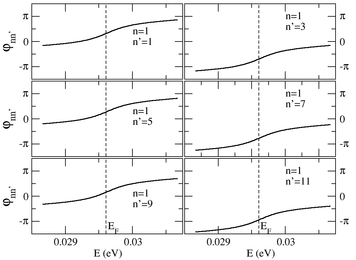
(a) (b)

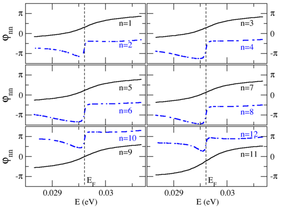
Figure 2: (Color online) Transmission phases between scattering channels with the same parity (solid black lines for odd channels and dot-dashed blue lines for the even ones): (a) $n=1$, $n^{\prime}=\overline{1,N_{F}}$ and (b) $n=n^{\prime}=\overline{1,N_{F}}$. The potential energy in the dot region is $V_{d}=V_{0}^{(1,2)}$ for which $E_{0}^{(1,2)}\simeq E_{F}$.

The phases associated with the odd scattering channels, $\varphi_{nn^{\prime}}$ with $n,n^{\prime}=1,3,...,11$, change slowly by $\pi$ in an energy interval comparable to the width of the resonance $(2,1)$, $\Gamma^{(2,1)}=6\cdot 10^{-4}$ eV, while for the even channels, the transmission phases show a total different evolution through the resonance $(1,2)$. They decrease slowly by approximatively $0.9\pi$ and increase after that abruptly to the initial value, similar to a phase lapseAvinun-Kalish et al. (2005); Oreg and Gefen (1997); Karrasch et al. (2007b); Oreg (2007) . For symmetry reasons the transmissions between odd and even scattering channels are forbidden.

Two conclusions are drawn from the plots in Fig. 2: i) the channel parity given by the parity of the function $\phi_{n}(y)$, Eq. (2), plays a decisive role in the transmission processes through an open quantum system and ii) the transmission phases between channels with the same parity show similar energy dependence in the energy domain of a resonance. So that, for a qualitative characterization of the phase variation through a resonance it is enough to analyze the phases $\varphi_{11}$ and $\varphi_{22}$. The measured transmission phase through the quantum system, a linear combination of all phases $\varphi_{nn^{\prime}}$, should be approximatively obtained as a linear combination of $\varphi_{11}$ and $\varphi_{22}$.

II.2 Resonances

The transport through an open quantum dot strongly coupled to the conducting leads is dominated by resonances. When the quantum system becomes open, the corresponding Hamilton operator becomes non-Hermitian Müller and Rotter (2009); Rotter (2009) and the eigenstates $E_{\lambda}$ of the closed dot become resonances with the complex energies $\bar{E}_{0\lambda}=E_{0\lambda}-i\Gamma_{\lambda}/2$, $\lambda\geq 1$. They are simple poles of the current scattering matrix ${\tilde{\mbox{${\mathbf{\cal{S}}}$}}}$, solutions of the equation $\det[{\bf 1}+i{\mathbf{\Omega}}]=0.$ As shown in Ref. Racec et al., 2010, the R-matrix formalism allows for a decomposition of ${\tilde{\mbox{${\mathbf{\cal{S}}}$}}}$ around $E_{\lambda}$ in which the resonant and the background parts are separated,

$${\tilde{\mbox{${\mathbf{\cal{S}}}$}}}(E)=2iu_{0}\frac{\mathbf{\Theta}\,\vec{\beta}_{\lambda}\,\vec{\beta}^{T}_{\lambda}\,\mathbf{\Theta}}{E-E_{\lambda}-\bar{\cal{E}}_{\lambda}(E)}+{\tilde{\mbox{${\mathbf{\cal{S}}}$}}}_{\lambda}(E),$$ (12)

where $\vec{\beta}_{\lambda}(E)=(\mathbf{1}+i\mathbf{\Omega}_{\lambda})^{-1}\vec{\alpha}_{\lambda}$ is an infinite column vector that characterizes the resonance $\lambda$, $\bar{\cal{E}}_{\lambda}(E)=-i\vec{\beta}^{T}_{\lambda}\cdot\vec{\alpha}_{\lambda}$ is a complex function which ensures the analyticity of the current scattering matrix for every real energy $E$ and the matrix $\mathbf{\Omega}_{\lambda}$ is obtained from $\mathbf{\Omega}$ taking out the $\lambda$ term, $\mathbf{\Omega}_{\lambda}=\mathbf{\Omega}-u_{0}\frac{\vec{\alpha}_{\lambda}\,\vec{\alpha}^{T}_{\lambda}}{E-E_{\lambda}}$. The background matrix

$${\tilde{\mbox{${\mathbf{\cal{S}}}$}}}_{\lambda}(E)=\mathbf{\Theta}\left[\mathbf{1}-2(\mathbf{1}+i\mathbf{\Omega}_{\lambda})^{-1}\right]\mathbf{\Theta}$$ (13)

has a similar expression to the scattering matrix $\tilde{\mbox{${\mathbf{\cal{S}}}$}}$, Eq. (4), and gives rise to a further decomposition in a resonant and a background term if a second resonance exists around the Fermi energy.

The position of the resonance $\bar{E}_{0\lambda}$ in the complex energy plane is determined as a solution of the equation

$$\bar{E}_{0\lambda}-E_{\lambda}-\bar{\cal{E}}_{\lambda}(\bar{E}_{0\lambda})=0.$$ (14)

There exists a resonance energy associated with every Wigner-Eisenbud energy and the above equation is solved numerically using an iterative procedure starting with $\bar{E}=E_{\lambda}$. This method gives all resonances supported by the open quantum system, even the very narrow ones associated with quasi-bound states mainly localized within the dot region or the very broad ones associated with modes mainly localized in the point contact regions, i.e. aperture modesRacec et al. (2010). Based on the analogy between the scattering functions at the resonance energy, $|\psi_{n}^{(s)}(E_{0\lambda};x,y)|^{2}$, and the eigenfunctions of the corresponding closed quantum dot, we associate a pair of quantum numbers $(n_{x},n_{y})$ with each resonance $\lambda$; $n_{x}$ denotes the number of the maxima of $|\psi_{n}^{(s)}(E_{0\lambda};x,y)|^{2}$ in the $x$-direction and $n_{y}$ the number of the maxima in the $y$-direction and $(x,y)$ are points in the dot region. As discussed in Ref. Racec et al., 2010, the index $\lambda$ of a resonance energy is only technically relevant, but has no physical meaning.

II.3 Fano Approximation

Based on the decomposition, Eq. (12), of the $\tilde{\mbox{${\mathbf{\cal{S}}}$}}$ matrix, the transmission probability between the channel $n$ in the source contact and the channel $n^{\prime}$ in the drain contact can be written as a sum of a resonant contribution and a background,

$$T_{nn^{\prime}}(E)=T_{res}^{(nn^{\prime})}(E)+T_{bg}^{(nn^{\prime})}(E)$$ (15)

for energies around a given resonance energy $E_{0\lambda}$. The first contribution to the transmission probability contains a resonant term singular at $E=\bar{E}_{0\lambda}$,

$$T_{res}^{(nn^{\prime})}(E)=\left|\frac{2i{\cal{Z}}_{1\lambda}^{(nn^{\prime})}(E)}{E-E_{\lambda}-\bar{\cal{E}}_{\lambda}(E)}+{\cal{Z}}_{2\lambda}^{(nn^{\prime})}(E)\right|^{2}-\left|{\cal{Z}}_{2\lambda}^{(nn^{\prime})}(E)\right|^{2}$$ (16)

and the slowly varying functions of energy in this term are defined as

$${\cal{Z}}_{1\lambda}^{(nn^{\prime})}(E)=\left|(\vec{\beta}_{\lambda})_{1n}\right|\left|(\vec{\beta}_{\lambda})_{2n^{\prime}}\right|$$ (17)

and

$${\cal{Z}}_{2\lambda}^{(nn^{\prime})}(E)=(\vec{\beta}^{*}_{\lambda})_{1n}(\mbox{\boldmath$\sigma$}_{\lambda})_{nn^{\prime}}(\vec{\beta}^{*}_{\lambda})_{2n^{\prime}}/{\cal{Z}}_{1\lambda}^{(nn^{\prime})}(E),$$ (18)

where $\mbox{\boldmath$\sigma$}_{\lambda}$ is the part of $\tilde{\mbox{${\mathbf{\cal{S}}}$}}_{\lambda}$ that contains the transmission amplitudes, $(\mbox{\boldmath$\sigma$}_{\lambda})_{nn^{\prime}}(E)=(\tilde{\mbox{${\mathbf{\cal{S}}}$}}_{\lambda})_{2n^{\prime},1n}(E)$; $\vec{\beta}^{*}_{\lambda}$ denotes the complex conjugate of $\vec{\beta}_{\lambda}$. The background term

$$T_{bg}^{(nn^{\prime})}(E)=\left|(\mbox{\boldmath$\sigma$}_{\lambda})_{nn^{\prime}}(E)\right|^{2}$$ (19)

is also a slowly varying function of energy around $E_{0\lambda}$, if a second resonance does not exist in the energy domain of the resonance $\lambda$.

As shown in Appendix A, the contribution of the resonance $\bar{E}_{0\lambda}$ to the transmission probability $T_{nn^{\prime}}$ can be approximated as a Fano line

$$T^{(nn^{\prime})}_{res}(E)\simeq T_{1nn^{\prime}}\left|\frac{1}{e_{\lambda}+i}+\frac{1}{q_{Fnn^{\prime}}}\right|^{2}-T_{2nn^{\prime}},$$ (20)

with a complex asymmetry parameter $q_{Fnn^{\prime}}$, where $e_{\lambda}=2(E-E_{0\lambda})/\Gamma_{\lambda}$. The constants $T_{1nn^{\prime}}$, $T_{2nn^{\prime}}$ and $q_{Fnn^{\prime}}$, computed using Eqs. (40), (41) and (42) respectively, depend actually on $\lambda$, but this index was omitted for simplicity. For an isolated resonance the background contribution to the conductance is approximated as a constant, $T_{bg}^{(nn^{\prime})}(E)\simeq T_{bg}^{(nn^{\prime})}(E_{0\lambda})$.

The Fano line is defined as the absolute value of an energy dependent complex function and, as presented in Appendix B, one can associate a phase

$$\varphi_{Fnn^{\prime}}=\arg\left(\frac{1}{e_{\lambda}+i}+\frac{1}{q_{Fnn^{\prime}}}\right),$$ (21)

with each Fano line. The Fano phase, $\varphi_{Fnn^{\prime}}$ is an energy dependent function that provides a good approximation for the phase of the transmission amplitude around a resonance,

$$\varphi_{nn^{\prime}}\simeq\varphi_{Fnn^{\prime}}+\varphi^{(0)}_{nn^{\prime}}.$$ (22)

The constant phase $\varphi^{(0)}_{nn^{\prime}}$ can not be determined in the limits of the considered approach, because the Fano line gives only a satisfactory description on the peak, without the information about the background. In Appendix B we have analyzed the Fano lines and the associated Fano phases for different values of the complex asymmetry parameter $q_{F}=(q_{r},q_{i})$. The phase evolution through a peak, Fig. 12, shows typical mesoscopic features as observed experimentally by Avinun-Kalish et al., Ref. Avinun-Kalish et al., 2005. For an asymmetry parameter $q_{F}$ with $q_{i}<-1$ the phase increases monotonically by $2\pi$, while for $q_{i}>-1$ there is no global variation of the phase through the Fano peak; The phase has a maximum and a minimum in the peak region and reaches the initial value far away from the peak. In the case $|q_{r}|\gg|q_{i}|$ typical phase lapses of $\pi$ occur, while for $|q_{i}|>|q_{r}|$ the maxima and minima are approximatively equal in amplitude and generally smaller than $\pi$. This last type of phase variation through a resonance is also reported by Avinun-Kalish et al., see Figs. 4(b) and 5(b) in Ref. Avinun-Kalish et al., 2005, and gives a direct experimental proof of the complex nature of the Fano asymmetry parameter. In the limit $q_{i}\rightarrow 0$, i.e. neglecting the breaking of the time reversal symmetry in open systems, the existence of the phase lapses can be explainedOreg (2007), but the whole variety of profiles in the phase evolution observed experimentally in the mesoscopic regime can not be obtained.

The analysis of the complex Fano function in Appendix B proves that the Fano phase is more sensitive to the value of the asymmetry parameter than the well-known real Fano function. If the phase evolution in the transmission peak region is known, the domain in the complex plane where the Fano asymmetry parameter takes values is considerably restricted and it can be more precisely computed as a fit parameter for the transmission probability. The Fano parameter contains information about the processes that accompany the scattering through the open quantum dot and a possible exact value of it leads to a better characterization of the transport properties through the system. A strong asymmetry of the Fano line ($|1/q_{F}|>1$) indicates a strong interaction between overlapping resonances due to channel mixingRacec et al. (2010). The quantum interference becomes dominant in this type of open systems that can not be anymore described in the frame of an effective one dimensional modelRacec et al. (2010). Supplementary, the imaginary part of the Fano asymmetry parameter reflects the decoherence processes induced in an open quantum system by the interaction with the conducting leadsClerk et al. (2001); Bärnthaler et al. (2010). Even for systems for which the dissipation can be neglected, the coupling of the quantum system to the environment allows for a decoherent dephasing in the limits of an unitary evolutionBärnthaler et al. (2010).

III Conductance and transmission phases

In the frame of a noninteracting model and for low temperatures the conductanceRacec et al. (2010) through an open quantum system is directly related to the total transmission, Eq. (10), at the Fermi energy,

$$G(V_{d})=\frac{e^{2}}{h}\,T(E_{F};V_{d}),$$ (23)

where $V_{d}$ is the potential energy experienced by the electrons within the quantum system. The transmission coefficients are determined, as shown in Sec. II, for a fixed value of $V_{d}$. In the case of a quantum dot confined within a very shallow quantum well , i.e. for a low occupancy of the dot, the conductance, Figs. 3 and 4, shows typical mesoscopic features: asymmetrical peaks and dips whose widths do not increase monotonically with the distance to the bottom of the quantum dot, $E_{F}-V_{d}$. They are associated with isolated resonances or with sets of overlapping resonancesRacec et al. (2010). For each such a peak and dip we define the potential energy $V_{0\lambda}=V_{0}^{(n_{x},n_{y})}$ for which the main resonance of the set participates to the conductance, i.e. the resonance energy matches the Fermi energy, $E_{0\lambda}=E_{0}^{(n_{x},n_{y})}\simeq E_{F}$. The main resonance, denoted by $\lambda$, is the thinnest one of the set of overlapping resonances at the Fermi energy. The other resonances of the set are indexed according to their widths by $\lambda^{\prime}$, $\lambda^{\prime\prime}$ and so on.

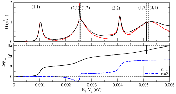
Figure 3: Upper part: Conductance (solid black line) and its Fano approximation (dashed red line) on each peak as a function of the potential energy in the dot region. Lower part: Phases of the transmission amplitudes between the scattering channels (1,n) and (2,n) with $n=1$ (black solid line) and $n=2$ (dot-dashed blue line). The phases for $V_{d}=E_{F}$ are set to $0$ in order to make evidently the phase variations of $\pi$.

To connect the peaks in the conductance to the resonances and to the scattering phases, one needs a functional dependence of the scattering matrix on $V_{d}$ around $V_{0}$; Here the index $\lambda$ is omitted for simplicity. A small variation $\delta V=V_{d}-V_{0}$ of the potential energy felt by the electron in the dot region can be approximately seen as a shift of the potential energy in the whole scattering area and, in turn, the conductance around $V_{0}$ becomesRacec et al. (2010)

$$G(V_{0}+\delta V)\simeq G_{res}(E_{F}-\delta V;V_{0})+G_{bg}(E_{F}-\delta V;V_{0}),$$ (24)

where the energy dependent functions $G_{res}$ and $G_{bg}$, given as

$$G_{res}(E)=\frac{e^{2}}{h}\left[\left|\frac{2i{\cal{Z}}_{1\lambda}(E)}{E-E_{\lambda}-\bar{\cal{E}}_{\lambda}(E)}+{\cal{Z}}_{2\lambda}(E)\right|^{2}-\left|{\cal{Z}}_{2\lambda}(E)\right|^{2}\right],$$ (25)

and

$$G_{bg}(E)=\frac{e^{2}}{h}\mbox{Tr}[\mathbf{\sigma}_{\lambda}(E)\mathbf{\sigma}_{\lambda}^{\dagger}(E)],$$ (26)

respectively, are exact expressions obtained from Eq. (12) without any approximation. The functions

$${\cal{Z}}_{1\lambda}(E)=\left|\vec{\beta}_{1\lambda}\right|\left|\vec{\beta}_{2\lambda}\right|$$ (27)

and

$${\cal{Z}}_{2\lambda}(E)=\vec{\beta}_{1\lambda}^{\dagger}\mathbf{\sigma}_{\lambda}\vec{\beta}_{2\lambda}^{*}/{\cal{Z}}_{1\lambda}(E)$$ (28)

are generally slowly varying in the energy domain of the resonance $\lambda$; $(\vec{\beta}_{1\lambda})_{n}=(\vec{\beta}_{\lambda})_{1n}$, $(\vec{\beta}_{2\lambda})_{n}=(\vec{\beta}_{\lambda})_{2n}$, and $({\mathbf{\sigma}}_{\lambda})_{nn^{\prime}}=({\tilde{\mathbf{\cal{S}}}}_{\lambda})_{1n,2n^{\prime}}$, $n\leq N_{1}(E_{F})$, $n^{\prime}\leq N_{2}(E_{F})$. Thus, the first contribution to the conductance, $G_{res}$, contains a resonant term singular at $E=\bar{E}_{0\lambda}$ and a term, ${\cal{Z}}_{2\lambda}(E)$, that describes the coupling of the resonance $\lambda$ characterized by the vector $\vec{\beta}_{\lambda}$ to the other resonances characterized by the background matrix $\mbox{\boldmath$\sigma$}_{\lambda}$. The second contribution to the conductance, $G_{bg}$, is given only by the background matrix $\mbox{\boldmath$\sigma$}_{\lambda}$ and it is approximatively constant in the case of an isolated resonance.

In the presence of the second resonance $\lambda^{\prime}\neq\lambda$ around the Fermi energy, the background contribution to the conductance, $G_{bg}$, has an energy dependence that can not be neglected anymore. The background term $\tilde{\mbox{${\mathbf{\cal{S}}}$}}_{\lambda}$ in $\tilde{\mbox{${\mathbf{\cal{S}}}$}}$, Eq. (12), can be further decomposedRacec et al. (2010) into a resonant term corresponding to the resonance $\lambda^{\prime}$ and a second background $\tilde{\mbox{${\mathbf{\cal{S}}}$}}^{\prime}_{\lambda}$ . Consequently, the term $G_{bg}$ in the expression Eq. (26) of the conductance is written as a sum of two contributions,

$$G_{bg}(E_{F}-\delta V;V_{0})=G^{\prime}_{res}(E_{F}-\delta V;V_{0})+G^{\prime}_{bg}(E_{F}-\delta V;V_{0}),$$ (29)

a resonant one,

$$G^{\prime}_{res}(E)=\frac{e^{2}}{h}\left[\left|\frac{2i{\cal{Z}}^{\prime}_{1\lambda}(E)}{E-E_{\lambda^{\prime}}-\bar{\cal{E}}^{\prime}_{\lambda}(E)}+{\cal{Z}}^{\prime}_{2\lambda}(E)\right|^{2}-\left|{\cal{Z}}^{\prime}_{2\lambda}(E)\right|^{2}\right],$$ (30)

and a second background

$$G^{\prime}_{bg}(E)=\frac{e^{2}}{h}\mbox{Tr}[\mathbf{\sigma}^{\prime}_{\lambda}(E)\mathbf{\sigma}_{\lambda}^{{}^{\prime}\dagger}(E)],$$ (31)

slowly varying with the energy if a third resonance does not exist around $E_{F}$, where $(\mbox{\boldmath$\sigma$}^{\prime}_{\lambda})_{nn^{\prime}}=(\tilde{\mbox{${\mathbf{\cal{S}}}$}}^{\prime}_{\lambda})_{2n,1n^{\prime}}$, $n,n^{\prime}\geq 1$. The functions ${\cal{Z}}^{\prime}_{1\lambda}$, ${\cal{Z}}^{\prime}_{2\lambda}$, and $\bar{\cal{E}}^{\prime}_{\lambda}$ are obtained from ${\cal{Z}}_{1\lambda}$, ${\cal{Z}}_{2\lambda}$, and $\bar{\cal{E}}_{\lambda}$ by replacing $\vec{\alpha}_{\lambda}$ by $\vec{\alpha}_{\lambda^{\prime}}$ and $\mathbf{\Omega}_{\lambda}$ by $\mathbf{\Omega}^{\prime}_{\lambda}=\mathbf{\Omega}_{\lambda}-u_{0}\frac{\vec{\alpha}_{\lambda^{\prime}}\,\vec{\alpha}^{T}_{\lambda^{\prime}}}{E-E_{\lambda^{\prime}}}$. In Eq. (29) the potential energy $V_{0}$ denotes $V_{0\lambda}$ corresponding to the thinest resonance of the set.

The expression Eq. (31) of the resonant contribution to the conductance allows for a new split up of this term in the case of three interacting resonances around the Fermi energy. The successive decomposition of the scattering matrix and, in turn, of the conductance, presented in this section is relevant as long as it is performed hierarchically, from the thinnest resonance to the broadest one and can be used for an arbitrary number of overlapping resonances.

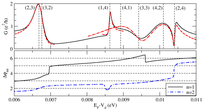
Figure 4: Upper part: Conductance (solid black line) and its Fano approximation (dashed red line) on each peak as a function of the potential energy in the dot region. Lower part: Phases of the transmission amplitudes between the scattering channels (1,n) and (2,n) with $n=1$ (solid black line) and $n=2$ (dot-dashed blue line). The phases for $V_{d}=E_{F}$ are set to $0$ in order to make evidently the phase variations of $\pi$.

III.1 Isolated resonances

In the case of an isolated resonanceRacec et al. (2010) around the Fermi energy, $\bar{E}_{0\lambda}\simeq E_{F}$, the contribution $G_{res}$ to the conductance, Eq. (25), is singular at $E=\bar{E}_{0\lambda}$ and yields always a peak mainly localized in the resonance domain. Following the method presented in Appendix A, this contribution can be approximated as a Fano line with the complex asymmetry parameter $q_{F\lambda}$,

$$G_{res}(E_{F}-\delta V) \simeq G_{1\lambda}\left|\frac{1}{v_{\lambda}+i}+\frac{1}{q_{F\lambda}}\right|^{2}-G_{2\lambda}$$ (32)

$$= G_{F}(E_{F}-\delta V),$$

where $v_{\lambda}=-2\delta V/\Gamma_{\lambda}$. The constants $G_{1\lambda}$ and $G_{2\lambda}$ as well as the Fano parameter $q_{F\lambda}$ are computed using Eqs. (41), (42) and (40), respectively. The background contribution to the conductance is approximated by a constant,

$$G_{bg}(E_{F}-\delta V)\simeq G_{bg}(E_{F})=G_{0}.$$ (33)

According to Eq. (32) the lowest approximation for a resonant peak in conductance through an open quantum dot is a Fano line with a complex asymmetry parameter. For huge values of this parameter, i.e. in the limit $|1/q_{F\lambda}|\ll 1$, the line shape becomes quasi Breit-Wigner. From the mathematical point of view, this situation corresponds to a very slow variation with the energy of the functions ${\cal{Z}}_{1\lambda}$ and $\bar{\cal{E}}_{\lambda}$. The condition is fulfilled only for an almost constant rest matrix ${\tilde{\mbox{${\mathbf{\cal{S}}}$}}}_{\lambda}$ in the energy domain of the resonance $\lambda$, i.e. if and only if the other resonances are far enough from the considered one. Supplementary, ${\tilde{\mbox{${\mathbf{\cal{S}}}$}}}_{\lambda}$ should have small values comparatively to the singular term in Eq. (12). In the presence of a weak interaction with other resonances $|1/q_{F\lambda}|$ increases and the corresponding line in the total transmission through the quantum dot becomes asymmetric.

Resonance	$q_{F}$	$q_{F11}$	$q_{F22}$
(1,1)	$9.399-1.003\,i$	$9.411-1.06\,i$	-
(1,2)	$50.45-1.013\,i$	-	$15.3+17.1\,i$
(2,1)	$13.38-1.049\,i$	$12.33-5.04\,i$	-
(2,2)	$144.7-1.052\,i$	-	$-0.47-21.1\,i$
(1,3)	$-0.23-1.0002\,i$	$-0.23-0.98\,i$	-
(3,1)	$11.29-1.248\,i$	$9.386-5.93\,i$	-
(2,3)	$-1.22-0.999\,i$	$-1.25-1.19\,i$	-
(3,2)	$-67.7-1.196\,i$	-	$-24.19+18.8\,i$
(1,4)	$3.144-1.001\,i$	-	$3.361-0.64\,i$
(4,1)	$9.78-1.197\,i$	$7.44-4.36\,i$	-
(3,3)	$-0.27-0.995\,i$	$-0.27-0.99\,i$	-
(2,4)	$0.52-1.003\,i$	-	$0.5-1.059\,i$
(4,2)	$-12.01-0.883\,i$	-	$-5.84-6.12\,i$

Table 1: Asymmetry parameters of the Fano profiles in conductance and in the transmission probabilities $T_{11}$ and $T_{22}$ for the indicated resonances.

The proposed approach works very well for the conductance peaks associated with isolated resonances like the first peak in Fig. 3. For the resonance (1,1) the function $G_{F}+G_{0}$, red dashed line in Fig. 3, computed for $V_{d}=V_{0}^{(1,1)}$ for which $E_{0}^{(1,1)}\simeq E_{F}$, provides an excellent approximation of the conductance on the peak. The Fano parameter of the function $G_{F}$, given in Tab. 1, corresponds to a slight asymmetry of the line shape. This behaviour is expected for an isolated resonance that interacts very weakly with the neighbor resonances and for which the Fano type interference is negligible.

The profile of the peak (1,1) and the climb by $\pi$ of the phase $\varphi_{11}$ in the energy domain of this peak, Fig. 3, could suggest that an approach by means of a Lorentzian is actually enough for describing isolated resonances. But the nonzero imaginary part of the asymmetry parameter $q_{F}$ requires a detailed analysis of the phases $\varphi_{11}$ and $\varphi_{F11}$, Eqs. (11) and (21), respectively. Around the resonance (1,1) the energy dependence of $\varphi_{F11}$ is similar to that plotted in Fig. 12 for $q_{r}=-50$ and $q_{i}=1.2$. However, around the maximum $(1,1)$, where the Fano approximation for the total transmission $T(E)$ works well, only one of the two variations of $\pi$ in the transmission phase occurs. The second step in $\varphi_{F11}$ is outside the plotted interval.

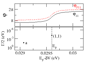
Figure 5: (Color online) Upper part: Transmission phase $\varphi_{11}$ (black full line) around the resonance $(1,1)$ and its Fano approximation $\varphi_{F11}$ (dashed red line). The difference between the two curves gives the constant phase $\varphi^{(0)}_{11}$. Lower part: Poles and position of the Fermi level in the complex energy plane for $V_{d}=V_{0}^{(1,1)}$.

As illustrated in Fig. 5, for the resonance (1,1) the Fano phase $\varphi_{F11}$ approximates excellently the transmission phase $\varphi_{11}$; The initial phase $\varphi_{11}^{(0)}$, Eq. (22), can not be determined, but it is not really relevant.

Around the resonance (1,1) the transmission phase $\varphi_{22}$ is practically constant, see Fig. 3, and this behaviour certifies also the odd parity of the resonant mode (1,1). In contrast, for the resonance (2,2), which is also an isolated one, the transmission phase $\varphi_{11}$ remains almost constant in the resonance domain and $\varphi_{22}$ increases by $\pi$. The slow variation of $\varphi_{11}$ around the resonance (2,2) is determined by the influence of the mode (3,1) that is very broad. Due to the symmetry reasons the modes (2,2) can not couple to the neighbor modes (2,1) and (3,1) and the resonance (2,2) shows the typical features of an isolated resonance.

III.2 Overlapping resonances

In the case of two overlapping resonances, $\bar{E}_{0\lambda}$ and $\bar{E}_{0\lambda^{\prime}}$ with $\Gamma_{\lambda^{\prime}}>\Gamma_{\lambda}$, around the Fermi energy, each of them yields a resonant contribution to the conductance, $G_{res}$ and $G^{\prime}_{res}$, Eqs. (25) and (30), respectively. The peak in the total transmissionRacec et al. (2010), a superposition of $G_{res}$ and $G^{\prime}_{res}$, has an asymmetric line shape and a maximum value different from 1. Similar to $G_{res}$, Eq. (32), the contribution $G^{\prime}_{res}$ of the second resonance can be also approximated as a Fano line

$$G^{\prime}_{res}(E_{F}-\delta V) \simeq G^{\prime}_{1\lambda}\left|\frac{1}{v^{\prime}_{\lambda}+i}+\frac{1}{q^{\prime}_{F\lambda}}\right|^{2}-G^{\prime}_{2\lambda}$$ (34)

$$= G^{\prime}_{F}(E_{F}-\delta V)$$

with $v^{\prime}_{\lambda}=2(E_{F}-\delta V-E_{0\lambda^{\prime}})/\Gamma_{\lambda^{\prime}}$. The complex asymmetry parameter $q^{\prime}_{F\lambda}$ of this line is obtained from Eq. (40) and the constants $G^{\prime}_{1\lambda}$ and $G^{\prime}_{2\lambda}$ from Eqs. (41) and (42), respectively. In the case of only two overlapping resonances, the second background contribution to the conductance is approximatively a constant,

$$G^{\prime}_{bg}(E_{F}-\delta V)\simeq G^{\prime}_{bg}(E_{F})=G^{\prime}_{0}.$$ (35)

The broader resonance $\lambda^{\prime}$ around the resonance $\lambda$ influences not only the background term $G_{bg}$ in the conductance, Eq. (24), but also the Fano asymmetry parameter $q_{F\lambda}$ associated with the first resonant term $G_{res}$, Eq. (32). The function ${\cal{Z}}_{2\lambda}$, Eq. (28), that enters $q_{F\lambda}$, Eq. (40), describes the interaction between resonances and can be also decomposed in a resonant term singular at $E=\bar{E}_{0\lambda^{\prime}}$ and a background term,

$${\cal{Z}}_{2\lambda}(E)=\frac{1}{{\cal{Z}}_{1\lambda}(E)}\left[\frac{\vec{\beta}_{1\lambda}^{\dagger}\cdot\vec{\beta}_{1\lambda^{\prime}}\,\vec{\beta}_{2\lambda}^{\dagger}\cdot\vec{\beta}_{2\lambda^{\prime}}}{E-E_{\lambda^{\prime}}-\bar{\cal{E}}^{\prime}_{\lambda}}+\vec{\beta}_{1\lambda}^{\dagger}\mbox{\boldmath$\sigma$}^{\prime}_{\lambda}\vec{\beta}_{2\lambda}^{*}\right].$$ (36)

The vector $\vec{\beta}_{\lambda}$ characterizes the resonance $\lambda$, $\vec{\beta}_{\lambda^{\prime}}$ the resonance $\lambda^{\prime}$ and $\mbox{\boldmath$\sigma$}^{\prime}_{\lambda}$ the other ones. The strength of the coupling between the two overlapping resonances is indicated by the scalar products $\vec{\beta}_{1\lambda}^{\dagger}\cdot\vec{\beta}_{1\lambda^{\prime}}$ and $\vec{\beta}_{2\lambda}^{\dagger}\cdot\vec{\beta}_{2\lambda^{\prime}}$; For resonant modes with the same symmetry the two vectors are approximatively parallel to each other, while for different symmetries they are quasi-orthogonal to each other. The resonant term in ${\cal{Z}}_{2\lambda}$ is dominant only for the same parity. If this condition is fulfilled $|1/q_{F\lambda}|$ becomes large and the transmission shows a strong asymmetric line shape or a dip. Thus, by a favorable parity two overlapping resonances define two interfering pathways responsible for the Fano effect. In the opposite situation, for resonant states $\lambda$ and $\lambda^{\prime}$ with different parities, the value of $|1/q_{F\lambda}|$ is quite small and the Fano line is almost symmetric. Therefore, the quantum interference of the two pathways plays a minimal role. However, the interference with other resonant pathways belonging to the background is not excluded.

If we perform further a drastic approximation in $1/q_{F\lambda}$, neglecting the derivatives of the first order of ${\cal{Z}}_{1\lambda}$ and $\bar{\cal{E}}_{\lambda}$, which are slowly varying functions of energy, we find

$$\frac{1}{q_{F\lambda}}\simeq-i\frac{i\Gamma_{\lambda}/2}{E_{0\lambda}-E_{0\lambda^{\prime}}+i\Gamma_{\lambda^{\prime}}/2}\left.\frac{\vec{\beta}_{1\lambda}^{\dagger}\cdot\vec{\beta}_{1\lambda^{\prime}}\,\vec{\beta}_{2\lambda}^{\dagger}\cdot\vec{\beta}_{2\lambda^{\prime}}}{\vec{\beta}_{1\lambda}^{\dagger}\cdot\vec{\beta}_{1\lambda}\,\vec{\beta}_{2\lambda}^{\dagger}\cdot\vec{\beta}_{2\lambda}}\right|_{E=E_{0\lambda}}.$$ (37)

In the case of a favorable symmetry the second fraction is approximatively 1 and the relative position of the two overlapping resonances in the complex energy plane determines the value of the asymmetry parameter $1/q_{F\lambda}$. For two resonances very close in energy, $E_{0\lambda}\simeq E_{0\lambda^{\prime}}$, the Fano parameter is a complex number with a large imaginary part comparatively to the real one. This property of the asymmetry parameter is the fingerprint of an unitary dephasing in a quantum system coupled to the environmentClerk et al. (2001); Bärnthaler et al. (2010) and can be directly seen in the phase of the Fano function. For different values of the Fano asymmetry parameter the phase shift is analyzed in Appendix B. Thus, based on a very simple model for the Fano asymmetry parameter, we can associate dephasing effects to overlapping resonances that interact strongly due to the same symmetry of the resonant modes.

Further we analyze different types of overlapping resonances and try to answer the question if the coupling between resonances always induces a decoherent dephasing or not. Is the absence of the Fano effect, i.e. a quasi symmetrical peak in the total transmission, an unambiguous proof of the phase coherence?

III.2.1 Weak interacting regime

In the weak coupling regime each resonance contributes to the conductance with a Fano line with a slight ($|1/q_{F}|\ll 1$) up to an intermediate ($|1/q_{F}|\simeq 1$) asymmetry, as plotted in Fig. 6(a) for the resonances (1,2) and (2,1). The Fano parameters of these lines, see Tab. 1, reflect the weak coupling of the resonances to each other and to the neighbor onesRacec et al. (2010). Because of its symmetry the resonant mode (1,2) is quasi isolated and the corresponding Fano line shows practically a Breit-Wigner profile. The parity of the resonant modes suppresses in this case the Fano effect. In contrast, the second mode, (2,1), interacts with the resonant mode (1,1) as well as with the very broad resonance (3,1). Its Fano line is slight asymmetric with $|1/q_{F}^{(2,1)}|>|1/q_{F}^{(1,2)}|$. Even in the case of a partial overlapping, a favorable parity of the resonant modes allows for quantum interference directly reflected by the asymmetry of the transmission peak.

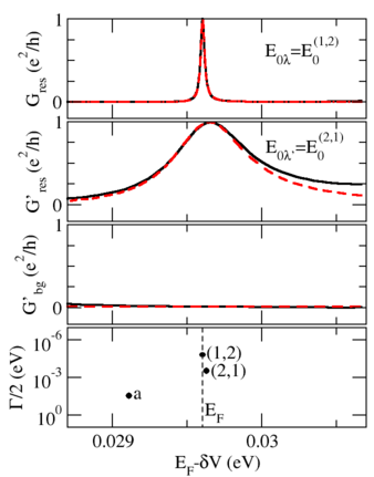
(a) (b)

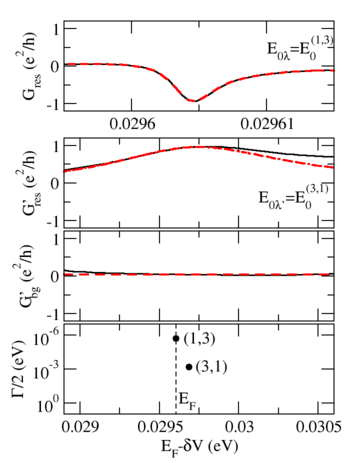
Figure 6: (Color online) Upper parts: Resonant contributions to the conductance $G_{res}$ and $G^{\prime}_{res}$ (solid black lines) and the corresponding Fano lines $G_{F}$ and $G^{\prime}_{F}$ (dashed red lines); Middle parts: Background contribution to the conductance $G^{\prime}_{bg}$ (solid black lines) and its constant approximation $G^{\prime}_{0}$ (dashed red lines). Lower parts: Poles and position of the Fermi level in the complex energy plane. The potential energy in the dot region is constant, (a) $V_{d}=V_{0}^{(1,2)}$ and (b) $V_{d}=V_{0}^{(1,3)}$.

Although the first Fano line is quasi-symmetric, the interaction between the resonances (1,2) and (2,1) is present and leads to their separation on the imaginary axisRacec et al. (2010). A second manifestation of this interaction is the decoherent dephasing of the resonant mode (1,2), directly observed in the transmission phase $\varphi_{22}$ plotted in Fig. 7(a). This phase presents a drop of about $\pi/2$ followed by a climb of $\pi$ through the resonance (1,2), while the phase $\varphi_{11}$ increases monotonically by $\pi$ through the resonance (2,1).

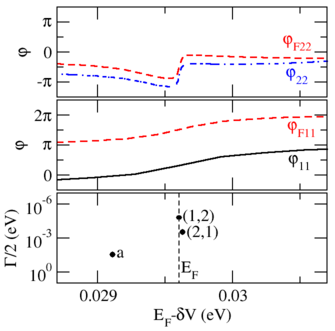
(a) (b)

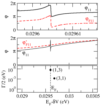
Figure 7: (Color online) Upper parts: Transmission phases $\varphi_{nn}$, (solid black lines for $n=1$ and dot-dashed blue line for $n=2$) and the Fano phases $\varphi_{Fnn}$ (red dashed lines) for the resonances (1,2) and (2,1) in (a) and (1,3) and (3,1) in (b). Lower parts: Poles and position of the Fermi level in the complex energy plane. The potential energy in the dot region is constant, (a) $V_{d}=V_{0}^{(1,2)}$ and (b) $V_{d}=V_{0}^{(1,3)}$.

To prove that the interaction of the overlapping resonances is responsible for dephasing, we analyze the imaginary part of the Fano asymmetry parameter associated with the transmission probability $T_{22}$, see Tab. 1. The value of this parameter, $|1/q_{F22}|\simeq 0.04$, corresponds to a quasi symmetric profile in $T_{22}$, similar to $G_{res}$ in Fig. 6(a), but the imaginary part of $q_{F22}$ is larger than the real one. According to the analysis in Appendix B the corresponding Fano phase $\varphi_{F22}$ shows a dip and not a monotonically increasing by $\pi$ as could be expected for a quasi Breit-Wigner line. The Fano phase $q_{F22}$ describes accurately the phase evolution through the resonance (1,2) as illustrated in Fig. 7(a). Also in the case of the resonance (2,1) the phase defined in the frame of the Fano approximation, $\varphi_{F11}$, describes very well the transmission phase $\varphi_{11}$; the associated asymmetry parameter is given in Tab. 1.

Here we have to remark, that, for some resonances, there is a difference between the Fano parameter $q_{F}$ associated with $T$ and the parameters $q_{F11}$ or $q_{F22}$ associated with $T_{11}$ or $T_{22}$, respectively. The total transmission $T$ describes a global effect, containing contributions from all scattering channels while $T_{11}$ and $T_{22}$ correspond only to the transmission between a pair of channels. As reported in Ref. Nakanishi et al., 2004, the global Fano parameter is given as a linear combination of the asymmetry parameters for each pair of scattering channels. Thus, the corresponding profiles in the transmission differ slightly from channel to channel and also from the total transmission.

A similar phase shift across the second peak in the conductance is observed experimentally by Kalish et al.Avinun-Kalish et al. (2005). They reported a dip in the transmission phase that always occurs in front of the second conductance maximum, i.e. before the entry of the second electron for the setup in that experiment. The drop of about $\pi/2$ is followed by a phase antilapseSilva et al. (2002) and these phase variations survive the changes in the system parameters. The experimental findings are especially interesting if we consider that the quantum dot used by Kalish et al. Avinun-Kalish et al. (2005) and the dot modelled by us have similar geometries but different electron densities. We can conclude that the phase antilapse associated with the overlapping resonances (1,2) and (2,1) is a general finding and it occurs independently of the quantum system parameters. Responsible for this phase evolution can be only the dephasing process induced by the interaction of the two overlapping resonances. While this interaction leads to the quantum interference and consequently to asymmetric Fano line in the total transmission only in the case of a favorable parity of the resonant modes, the dephasing is present even for the weak coupling regime of the overlapping resonances.

A second antilapse in the transmission phase, also a so-called nonuniversal oneBaksmaty et al. (2008), occurs in the energy domain of the resonance (1,4), as plotted in Fig. 8. For this resonance the Fano asymmetry parameter $q_{F22}$, Tab. 1, indicates a slight asymmetry of the transmission line $T_{22}$ and an approximative symmetrical dip of about $3\pi/4$ in the transmission phase $\varphi_{F22}$. Also in this case the decoherent dephasing of the resonant modes (1,4) and (4,1) occurs as an effect of the interaction between resonances, accompanied by the separation of the two resonances on the imaginary axisRacec et al. (2010).

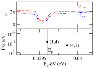
Figure 8: (Color online) Upper part: Transmission phase $\varphi_{22}$ (dot-dashed blue line) and the Fano phase $\varphi_{F22}$ (red dashed line). Lower parts: Poles and position of the Fermi level in the complex energy plane. The potential energy in the dot region is constant, $V_{d}=V_{0}^{(1,4)}$.

In contrast, the weakly interacting resonances (2,3) and (3,2) yield an asymmetric peak in conductance, but no phase lapse or antilapse in the energy domain of this peak, see Fig. 4. The reason is the relative large width of the resonance (3,2) that leads to a broad maximum in the transmission phase from which only a part is included in the energy domain of the transmission peak, as plotted in Fig. 9. The Fano approximation for the total transmission and for the transmission phases works also in this case very well.

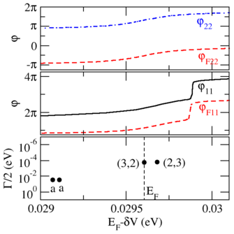
Figure 9: (Color online) Upper parts: Transmission phases $\varphi_{22}$ (dot-dashed blue line) and $\varphi_{11}$ (solid black line) and the Fano phases $\varphi_{F11}$ and $\varphi_{F22}$ (red dashed lines). Lower part: Poles and position of the Fermi level in the complex energy plane. The potential energy in the dot region is constant, $V_{d}=V_{0}^{(3,2)}$.

III.2.2 Strong interacting regime

Opposite to the weak interaction regime, the strong interaction between overlapping resonances requires the same parity in the lateral direction of the corresponding resonant modes. As analyzed in Ref. Racec et al., 2010, the strong resonance coupling leads to the hybridization of the resonant modes and to a strong repulsion of the resonances in the complex energy plane, i.e. a resonance trappingRotter (2009); Müller and Rotter (2009). In turn, strong localized resonant states, i.e. quasi-bound states, occur accompanied by broad ones, all of them with probability distribution densities in the dot region without correspondent between the eigenstates of an isolated dotRacec et al. (2010). The conductance peak associated with two strong interacting resonances is generally the superposition of a thin dip and a broad slight asymmetric maximum, as plotted in Fig. 6(b) for the resonances (1,3) and (3,1). The dip in conductance corresponding to the resonance (1,3) is characterized by a large absolute value of $|1/q_{F}|$, Tab. 1, reflecting the presence of the quantum interference. The real energies of the resonances (1,3) and (3,1) are very close and they define two interfering pathways for the transmission through the quantum system. The first path corresponds to the narrow resonance, while the second one is associated with a continuum of states in the energy domain of the second broad resonance. For this reason we can speak about a Fano type interference in open quantum systems strongly coupled to the environment.

A second effect associated with interacting resonances is the nondissipative dephasing induced on the resonant modes. As illustrated in the upper part of Fig. 7(b), in the energy domain of the resonance (1,3) the transmission phase $\varphi_{11}$ increases by $\sim\pi/2$, shows after that a phase lapse of $-\pi$ and increases again to the initial value. The phase variation of $\varphi_{11}$ is excellently described by the Fano phase. The imaginary part of the asymmetry parameter $q_{F11}$, Tab. 1, exceeds the real one and this peculiarity indicates the presence of the dephasing process in the case of interacting resonances, irrespective of the coupling strength between them. The value of the complex asymmetry parameter $q_{F11}$ for the resonance (1,3) corresponds to a lapse in the phase $\varphi_{F11}$ with a mesoscopic character. In contrast to the universal phase lapses, the nonuniversal ones depend on the dot occupancy.

The broad resonance (3,1) yields a supplementary variation of the phase $\varphi_{11}$ by $\pi$ within a much larger energy interval than the energy domain of the resonance (1,3). The phase $\varphi^{\prime}_{F11}$, Fig. 7(b) middle part, approximates also well the second slowly variation in $\varphi_{11}$. Opposite to the case of weakly interacting resonances, in the strong coupling regime both resonances determine variations of the same transmission phase. Thus, for the resonances (1,3) and (3,1) the transmission coefficients between odd scattering channels show phase variations, while in the case of the resonances (2,4) and (4,2) only for the even channels the phase is shifted through the overlapping resonances.

In Ref. Racec et al., 2010 we have already shown, that the overlapping resonances (2,4) and (4,2) interact strongly to each other and they are associated with typical hybrid resonant modes. But each effort to decompose the conductance in only two resonant contributions and a background was unavailing. Increasing the dot occupancy, increases also the resonant level density around the Fermi energy and there are more than two resonances that overlap and interact. For $V_{d}=V_{0}^{(2,4)}$ the four resonances that overlap are plotted in the lower part of Fig. 10.

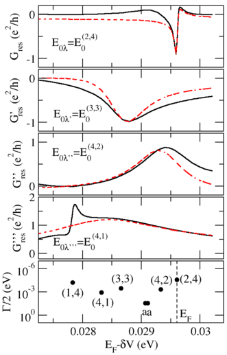
Figure 10: (Color online) Upper parts: Resonant contributions to the conductance $G_{res}$, $G^{\prime}_{res}$, $G^{\prime\prime}_{res}$ and $G^{\prime\prime\prime}_{res}$ (solid black lines) and the corresponding Fano lines $G_{F}$, $G^{\prime}_{F}$, $G^{\prime\prime}_{F}$ and $G^{\prime\prime\prime}_{F}$ (dashed red lines); The background contribution is $G^{\prime\prime\prime}_{0}=0.36\,e^{2}/h$. Lower part: Poles and position of the Fermi level in the complex energy plane for $V_{d}=V_{0}^{(2,4)}$.

The first contribution to the conductance is given by the resonance (2,4). This is the thinest one, followed by the resonances (3,3), (4,2) and (4,1) with $\Gamma^{(2,4)}<\Gamma^{(3,3)}<\Gamma^{(4,2)}<\Gamma^{(4,1)}$. This arrangement is determined by the existence of two pairs of strongly interacting resonances: (2,4) and (4,2) and (3,3) and (4,1), respectively. Corresponding to the strong interactions the first two contribution to the conductance, $G_{res}$ and $G^{\prime}_{res}$, are minima described by Fano lines. They are plotted in the upper parts of Fig. 10. Comparatively to the pair of strong interacting resonances (1,3) and (3,1), Fig. 6(b), in this case the first dip in conductance is broader because the strong interaction between the resonances (2,4) and (4,2) is perturbed by their weak coupling to the resonance (3,3). The other two contributions to the conductance, $G^{\prime\prime}_{res}$ and $G^{\prime\prime\prime}_{res}$ in Fig. 10, are broad maxima described also by Fano lines. The conductance is obtained in this case as a superposition of four Fano lines and a constant background. The asymmetry parameters of the Fano lines are given in Tab. 1. As illustrated in Fig. 4, the Fano approximation is satisfactory even in the case of four overlapping resonances and validates the description of the open quantum systems in terms of resonances. Due to the mutual interactions, the overlapping resonances are spread out into the complex energy plane so that there exists always a hierarchy of the resonances and the decomposition in successive Fano lines can be done. The asymmetry parameter of each line gives information about the coupling strength of the associated resonance to the other ones and, implicitly, about the presence or not of the quantum interference.

In the case of the four overlapping resonances analyzed above, the transmission phase $\varphi_{11}$ associated with odd channels as well as the phase $\varphi_{22}$ associated with the even ones show variations around the Fermi energy.

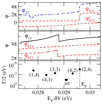
Figure 11: (Color online) Upper parts: Transmission phases $\varphi_{22}$ (dot-dashed blue line) and $\varphi_{11}$ (solid black line) and the Fano phases $\varphi_{F11}$, $\varphi_{F22}$, $\varphi^{\prime}_{F22}$ and $\varphi^{\prime}_{F11}$ (dashed red lines) associated with the resonances (2,4), (3,3), (4,2) and (4,1), respectively. Lower part: Poles and position of the Fermi level in the complex energy plane for $V_{d}=V_{0}^{(2,4)}$.

The Fano phase $\varphi_{F22}$ determined by the asymmetry parameter $q_{F22}$ corresponding to the resonance (2,4), Tab. 1, approximates very well the abrupt jump of $2\pi$ in the transmission phase $\varphi_{22}$. The second slow variation of $\pi$ in $\varphi_{22}$, superimposed on the jump, is determined by the resonance (4,2). This shift is also well described in the frame of the Fano approximation, as illustrated in the upper part of Fig. 11. The strongly interacting resonances (3,3) and (4,1) determine in $\varphi_{11}$ a nonuniversal phase lapse superimposed also on a slowly variation of $\pi$ associated with the broader resonance, see middle part of Fig. 11. The Fano asymmetry parameters corresponding to the resonances (3,3) and (4,1) are given in Tab. 1. The Fano phases $\varphi_{F11}$ and $\varphi^{\prime}_{F11}$ associated with these parameters approximate well the phase shift of $\varphi_{11}$.

IV Conclusions

In this paper we study the transmission probabilities and phases of noninteracting spinless electrons transfered through an open quantum dot strongly coupled to the conducting leads. The mechanism that governs the transport properties in the strong coupling regime is the interaction between overlapping resonances. Due the coupling of the quantum system to the environment, a degenerate or quasi-degenerate energy level evolves to two overlapping resonances that interact. As a consequence of the interaction the two resonances are separated in the complex energy plane and the corresponding resonant modes are dephased with respect to each other. The induced dephasing is the necessary condition for the quantum interference, but this condition is not sufficiently. The Fano effect requires supplementary a favorable parity of the resonant modes.

Using a model based on the scattering theory and the R-matrix formalism, we propose a successive decomposition of the total transmission in contributions corresponding to each resonance of the overlapping ones. Each contribution is approximated as a Fano line with a complex asymmetry parameter. The imaginary part of the Fano parameter gives information about the dephasing degree of the corresponding resonant modes, while its modulus characterizes the quantum interference with the other resonant modes.

The effects of the interaction between resonances can be directly seen in the measurable quantities conductance and transmission phases through the open quantum dot. In the frame of the Fano approximation we provide a very good description of the dips in conductance superimposed on broad maxima and accompanied by nonuniversal lapses in the transmission phases. We analyze mainly the mesoscopic regime characterized by a low occupancy of the quantum dot for which only two resonances interact. We associate the strong coupling between resonances with the Fano effect, while in the weak coupling regime only the shift of the transmission phases indicates the presence of their interaction. By increasing further the dot occupancy a set of many overlapping resonances lies around the Fermi energy and participates to the transport. The resonances interact with each other and determine complex line shapes in conductance and many transmission phase lapses. We can speak about the crossover regime between the mesoscopic and the universal oneAvinun-Kalish et al. (2005). For a proper characterization of this regime we have also to consider the Coulomb interaction that becomes nonnegligible by increasing the number of the electrons within the dot region. This subject will be studied in the future.

Appendix A Laurent expansion of the resonant term around the pole

We consider the general form of the resonant term in transmission as a complex function

$$f(E)=\frac{2iz_{1\lambda}(E)}{E-E_{\lambda}-\bar{e}_{\lambda}(E)}-z_{2\lambda}(E),$$ (38)

with a simple pole at $E=\bar{E}_{0\lambda}$ and with $\bar{e}_{\lambda}$, $z_{1\lambda}$ and $z_{2\lambda}$ slowly varying functions in the energy domain of the resonance $\lambda$.

To obtain the line shape of the total transmission, $F(E)=|f(E)|^{2}$, around the considered resonance, we extend the function $f(E)$ by analytic continuation in the lower part of the complex energy plane and employ a formal expansion of it in a Laurent series around the pole. The slow variation with the energy of the functions $\bar{e}_{\lambda}$, $z_{1\lambda}$ and $z_{2\lambda}$ around the resonance $\lambda$ allows to neglect their derivatives at the resonance energy up to the second orderRacec and Wulf (2001). Thus, for energy around $E_{0\lambda}$, the function $F(E)$ can be approximated as a Fano line

$$F(E)\simeq F_{1\lambda}\left|\frac{1}{e_{\lambda}+i}+\frac{1}{q_{F\lambda}}\right|^{2}-F_{2\lambda},$$ (39)

where $e_{\lambda}=2(E-E_{0\lambda})/\Gamma_{\lambda}$. The Fano asymmetry parameter $q_{F\lambda}$ is a complex number defined as

$$\frac{1}{q_{F\lambda}}=i\left.\left[\frac{dz_{1\lambda}}{dE}-i\frac{z_{2\lambda}}{2}\left(1-\frac{d\bar{e}_{\lambda}}{dE}\right)\right]\left[\frac{dz_{1\lambda}}{dE}+i\frac{z_{1\lambda}}{\Gamma_{\lambda}/2}\right]^{-1}\right|_{E=E_{0\lambda}}$$ (40)

and the constants $F_{1\lambda}$ and $F_{2\lambda}$ have the expressions

$$F_{1\lambda}=\left.\left|\frac{dz_{1\lambda}}{dE}+i\frac{z_{1\lambda}}{\Gamma_{\lambda}/2}\right|^{2}\left|1-\frac{d\bar{e}_{\lambda}}{dE}\right|^{-2}\right|_{E=E_{0\lambda}}$$ (41)

and

$$F_{2\lambda}=\left|z_{2\lambda}(\bar{E}_{0\lambda})\right|^{2},$$ (42)

respectively.

We have already used this approach to determine the conductance around an isolated resonance in the case of a separable confinement potential in the dot region, i.e. for an effective 1D systemRacec and Wulf (2001). But for the 2D case, the complex function $\bar{\cal{E}}_{\lambda}(E)$, which assures the analyticity of the resonant term, Eq. (12), becomes a product of two infinite vectors $\vec{\alpha}_{\lambda}$ and $\vec{\alpha}_{\lambda}^{T}$ with the infinite matrix $(1+i\mathbf{\Omega_{\lambda}})^{-1}$. For the numerical calculations we have to cut $\vec{\alpha}_{\lambda}$ and $\mathbf{\Omega_{\lambda}}$. The confinement potential of the quantum dot analyzed here has no attractive characterSimon (1976) and the influence of the evanescent channels can be neglected in this caseRacec et al. (2009). As usually done in the Landauer-Büttiker formalismBüttiker et al. (1985); Büttiker (1986), we have considered only the contributions of the open channels, i.e. a $2N_{F}$ vector $\vec{\alpha}_{\lambda}$ and a $2N_{F}\times 2N_{F}$ $\mathbf{\Omega_{\lambda}}$ matrix, where $N_{F}=N_{1}(E_{F})=N_{2}(E_{F})$.

Appendix B Fano functions

The complex Fano function is defined as

$$f_{c}(e)=\frac{1}{e+i}+\frac{1}{q_{F}}=\frac{1}{|q_{F}|}\,\sqrt{f(e)}\,e^{i\varphi_{F}},$$ (43)

where $q_{F}=(q_{r},q_{i})$ is a nonzero complex number usually called asymmetry parameter. This parameter is responsible for the asymmetry of the real Fano functionFano (1961); Fano and Rau (1986)

$$f(e)=\frac{|e+q|^{2}}{e^{2}+1},$$ (44)

with $q=q_{F}+i$. For each value of the parameter $q_{F}$ the function $f(e)$ has a maximum and a minimum,

$$M=1+\frac{q_{r}}{e_{M}}=f(e_{M})\quad\text{and}\quad m=1+\frac{q_{r}}{e_{m}}=f(e_{m})$$

respectively, for

$$e_{M,m}=-\frac{1}{2q_{r}}\left[2q_{i}+|q_{F}|^{2}\mp\sqrt{(2q_{i}+|q_{F}|^{2})^{2}+4q_{r}^{2}}\right].$$ (45)

In the limit $|1/q_{F}|\rightarrow 0$ the function $f(e)$ reduces to the Breit-Wigner form with a maximum at the origin, $e_{M}\rightarrow 0$, and a minimum at infinity, $e_{m}\rightarrow\infty$.

The phase of the complex Fano function is determined from the equation

$$\tan(\varphi_{F})=-\frac{q_{i}(e^{2}+1)+|q_{F}|^{2}}{q_{r}(e^{2}+1)+|q_{F}|^{2}e}$$ (46)

in which $q_{F}$ enters as a parameter. As plotted in Fig. 12, the phase dependence on $e$ varies strongly with the value of the Fano asymmetry parameter. Further we provide a systematic analysis of the function $\tan(\varphi_{F})$ in order to predict the phase evolution in the domain of a Fano line for a given value of $q_{F}$. From symmetry reasons $\tan[\varphi_{F}(e;q_{r},q_{i})]=-\tan[\varphi_{F}(-e;-q_{r},q_{i})]$ and we have plotted only the curves for $q_{r}<0$.

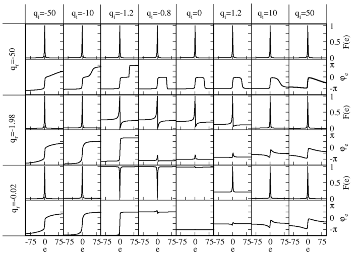
Figure 12: Fano function $F(e)=f(e)/M$ and the phase $\varphi_{F}$ of the complex Fano function, Eq. (43), for different values of the Fano asymmetry parameter $q_{F}=(q_{r},q_{i})$.

According to Eq. (46), $\lim_{e\rightarrow\pm\infty}\tan(\varphi_{F})=-q_{i}/q_{r}=\tan(\varphi_{\infty})$ and, consequently, the phase $\varphi_{F}$ has equal values at $e\rightarrow\pm\infty$ or shows a global variation of $2m\pi$, $m\geq 1$ along the $e$ axis. Because the function $\tan(\varphi_{F})$ has only two zeros at $e_{z\pm}=\pm\sqrt{-|q_{F}|^{2}/q_{i}-1}$ for

$$q_{F}\in\{(q_{r},q_{i})\in{\bf C},\,q_{r}^{2}+(q_{i}+1/2)^{2}>1/4\},$$ (47)

and only two poles at $e_{p\pm}=-(|q_{F}|^{2}\mp\sqrt{|q_{F}|^{4}-4q_{r}^{2}})/2q_{r}$ for

$$q_{F}\in\{(q_{r},q_{i})\in{\bf C},\,(1-|q_{r}|)^{2}+q_{i}^{2}>1\}$$ (48)

the phase shift can not exceed $2\pi$. To differentiate further between the cases that correspond to a global variation of $2\pi$ in $\varphi_{F}$ and the cases for which $\lim_{e\rightarrow-\infty}(\varphi_{F})\simeq\lim_{e\rightarrow\infty}(\varphi_{e})$, it is necessary to analyze the monotonicity of $\tan(\varphi_{F})$. For

$$q_{F}\in\{(q_{r},q_{i})\in{\bf C},\,q_{i}>-1\},$$ (49)

the first derivative of $\tan(\varphi_{F})$ has two zeros at $e_{m\pm}=\left[q_{r}\mp\sqrt{(1+q_{i})|q_{F}|^{2}}\right]/q_{i}$ and they correspond to a minimum and a maximum of this function, $\tan[\varphi_{F}(e_{m\pm})]=2q_{r}e_{m\pm}\tan(\varphi_{\infty})/(2q_{r}e_{m\pm}+|q_{F}|^{2})$. The phase variation between the maximum and the minimum values, Fig.12, depends strongly on $q_{F}$, but it can not exceed $\pi$. The limit value is obtained for $|q_{F}|\gg 1$. In the case $q_{i}\ll|q_{r}|$, $|q_{r}|\gg 1$ the phase increases from $0$ to $\pi$, has a plateau and decreases approximatively to $0$, while in the case $|q_{r}|\ll q_{i}$, $q_{i}\gg 1$ the phase decreases from $-\pi/2$ to $-\pi$, increases after that to $0$ and decreases further to $-\pi/2$. For smaller values of the Fano parameter for which the asymmetry of the Fano line is strong, $|q_{F}|\leq 1$, the phase does not vary strongly.

Opposite to this situation is the phase variation for $q_{i}<-1$. In this case $d\tan(\varphi_{F})/de$ has no zeros and, in turn, $\tan(\varphi_{F})$ increases monotonically with $e$. The phase shows a global variation of $2\pi$. Depending on the values of the Fano asymmetry parameter $|q_{F}|$, there is a jump of $2\pi$ or two steps of $\pi$ centered on $e_{p+}$ and $e_{p-}$. Actually the first case is a limit of the second one for a very small distance between $e_{p+}$ and $e_{p-}$.

The systematic analysis of the complex Fano function, Eq. (43), has shown that the phase of this function changes strongly by relative small variation of the real or the imaginary part of the asymmetry parameter. Even in the case of quasi-symmetrical Fano lines, $|1/q_{F}|\ll 1$, the quotient $q_{i}/q_{r}$ and the sign of $q_{i}$ yield a large variety of profiles in the phase evolution.

References

- Fano (1961) U. Fano, Phys. Rev. 124, 1866 (1961).
- Fano and Rau (1986) U. Fano and A. P. Rau, Atomic Collisions and Spectra (Academic Press, Orland, 1986).
- Miroshnichenko et al. (2010) A. E. Miroshnichenko, S. Flach, and Y. S. Kivshar, Rev. Mod. Phys. 82, 2257 (2010).
- Adair et al. (1949) R. K. Adair, C. K. Bockelman, and R. E. Peterson, Phys. Rev. 76, 308 (1949).
- Cedeira et al. (1973) F. Cedeira, T. A. Fjeldly, and M. Cardona, Phys. Rev. B 8, 4734 (1973).
- Faist et al. (1997) J. Faist, F. Capasso, C. Sirtori, K. W. West, and L. N. Pfeiffer, Nature (London) 390, 589 (1997).
- Göres et al. (2000) J. Göres, D. Goldhaber-Gordon, S. Heemeyer, M. A. Kastner, H. Shtrikman, D. Mahalu, and U. Meirav, Phys. Rev. B 62, 2188 (2000).
- Kobayashi et al. (2002) K. Kobayashi, H. Aikawa, S. Katsumoto, and Y. Iye, Phys. Rev. Lett. 88, 256806 (2002).
- Kobayashi et al. (2003) K. Kobayashi, H. Aikawa, S. Katsumoto, and Y. Iye, Phys. Rev. B 68, 235304 (2003).
- Kroner et al. (2008) M. Kroner, A. O. Govorov, S. Remi, B. Biedermann, S. Seidl, A. Badolato, P. M. Petroff, W. Zhang, R. Barbour, B. D. Gerardot, et al., Nature 451, 311 (2008).
- O.Entin-Wohlman et al. (2002) O.Entin-Wohlman, A.Aharony, Y.Imry, and Y. Levinson, J. Low. Temp. Phys. 126, 1251 (2002).
- Nakanishi et al. (2004) T. Nakanishi, K. Terakura, and T. Ando, Phys. Rew. B 69, 115307 (2004).
- Kobayashi et al. (2004) K. Kobayashi, H. Aikawa, A. Sano, S. Katsumoto, and Y. Iye, Phys. Rev. B 70, 035319 (2004).
- Sato et al. (2005) M. Sato, H. Aikawa, K. Kobayashi, S. Katsumoto, and Y. Iye, Phys. Rev. Lett. 95, 066801 (2005).
- Avinun-Kalish et al. (2005) M. Avinun-Kalish, M. Heilblum, O. Zarchin, D. Mahalu, and V. Umansky, Nature 436, 529 (2005).
- Nöckel and Stone (1994) J. U. Nöckel and A. D. Stone, Phys. Rev. B 50, 17415 (1994).
- Nöckel and Stone (1995) J. U. Nöckel and A. D. Stone, Phys. Rev. B 51, 17219 (1995).
- Clerk et al. (2001) A. A. Clerk, X. Waintal, and P. W. Brouwer, Phys. Rev. Lett. 86, 4636 (2001).
- Racec and Wulf (2001) E. R. Racec and U. Wulf, Phys. Rev. B 64, 115318 (2001).
- Racec et al. (2002) P. N. Racec, E. R. Racec, and U. Wulf, Phys. Rev. B 65, 193314 (2002).
- Magunov et al. (2003) A. I. Magunov, I. Rotter, and S. I. Strakhova, Phys. Rev. B 68, 245305 (2003).
- Johnson et al. (2004) A. C. Johnson, C. M. Marcus, M. P. Hanson, and A. C. Gossard, Phys. Rev. Lett. 93, 106803 (2004).
- Moldoveanu et al. (2005) V. Moldoveanu, M. Ţolea, V. Gudmundsson, and A. Manolescu, Phys. Rev. B 72, 085338 (2005).
- Satanin and Joe (2005) A. M. Satanin and Y. S. Joe, Phys. Rev. B 71, 205417 (2005).
- Mendoza et al. (2008) M. Mendoza, P. A. Schulz, R. O. Vallejos, and C. H. Lewenkopf, Phys. Rev. B 77, 155307 (2008).
- K.Ferry et al. (2009) D. K.Ferry, S. M. Goodnick, and J. Bird, Transport in Nanostructures (Cambridge University Press, Cambridge, 2009).
- Racec et al. (2010) E. R. Racec, U. Wulf, and P. N. Racec, Phys. Rev. B 82, 085313 (2010).
- Karrasch et al. (2007a) C. Karrasch, T. Hecht, A. Weichselbaum, Y. Oreg, J. von Delft, and V. Meden, New J. Phys. 9, 123 (2007a).
- Karrasch et al. (2007b) C. Karrasch, T. Hecht, A. Weichselbaum, Y. Oreg, J. von Delft, and V. Meden, Phys. Rev. Lett. 98, 186802 (2007b).
- Oreg (2007) Y. Oreg, New J. Phys. 9, 122 (2007).
- Yacoby et al. (1995) A. Yacoby, M. Heiblum, D. Mahalu, and H. Shtrikman, Phys. Rev. Lett. 74, 4047 (1995).
- Schuster et al. (1997) R. Schuster, E. Buks, M. Heilblum, D. Mahalu, V. Umansky, and H. Shtrikman, Nature 385, 417 (1997).
- Katsumoto (2007) S. Katsumoto, J. Phys.: Condens. Matter 19, 233201 (2007).
- Hackenbroich and Weidenmüller (1996) G. Hackenbroich and H. A. Weidenmüller, Phys. Rev. Lett. 76, 110 (1996).
- Oreg and Gefen (1997) Y. Oreg and Y. Gefen, Phys. Rev. B 55, 13726 (1997).
- Lee (1999) H.-W. Lee, Phys. Rev. Lett. 82, 2358 (1999).
- Levy and Büttiker (2000) Y. A. Levy and M. Büttiker, Phys. Rev. B 62, 7307 (2000).
- Silva et al. (2002) A. Silva, Y. Oreg, and Y. Gefen, Phys. Rev. B 66, 195316 (2002).
- Golosov and Gefen (2006) D. I. Golosov and Y. Gefen, Phys. Rev. B 74, 205316 (2006).
- Bertoni and Goldoni (2007) A. Bertoni and G. Goldoni, Phys. Rev. B 75, 235318 (2007).
- Müller and Rotter (2009) M. Müller and I. Rotter, Phys. Rev. A 80, 042705 (2009).
- Hecht et al. (2009) T. Hecht, A. Weichselbaum, Y. Oreg, and J. von Delft, Phys. Rev. B 80, 115330 (2009).
- Ţolea et al. (2010) M. Ţolea, M. Niţa, and A. Aldea, Physica E 42, 2231 (2010).
- Goldhaber-Gordon et al. (1998) D. Goldhaber-Gordon, H. Shtrikman, D. Mahalu, D. Abusch-Magder, U. Meirav, and M. Kastner, Nature 391, 156 (1998).
- Racec et al. (2009) P. N. Racec, E. R. Racec, and H. Neidhardt, Phys. Rev. B 79, 155305 (2009).
- Wulf et al. (1998) U. Wulf, J. Kučera, P. N. Racec, and E. Sigmund, Phys. Rev. B 58, 16209 (1998).
- Rotter (2009) I. Rotter, J. Phys. A: Math. Theor. 42, 153001 (2009).
- Bärnthaler et al. (2010) A. Bärnthaler, S. Rotter, F. Libisch, J. Burgdörfer, S. Gehler, U. Kuhl, and H.-J. Stöckmann, Phys. Rev. Lett. 105, 056801 (2010).
- Baksmaty et al. (2008) L. O. Baksmaty, C. Yannouleas, and U. Landman, Phys. Rev. Lett. 101, 136803 (2008).
- Simon (1976) B. Simon, Ann. Physics 97, 279 (1976).
- Büttiker et al. (1985) M. Büttiker, Y. Imry, R. Landauer, and S. Pinhas, Phys. Rev. B 31, 6207 (1985).
- Büttiker (1986) M. Büttiker, Phys. Rev. Lett. 57, 1761 (1986).