Pairing Fluctuations and Anomalous Transport Above the BCS-BEC Crossover
in the Two Dimensional Attractive Hubbard Model

Abstract

A Fermi liquid with weak attractive interaction undergoes a BCS transition to a superconductor with reducing temperature. With increasing interaction strength, the thermal transition is progressively modified as the high temperature ‘metallic’ phase develops a pseudogap due to pairing fluctuations and the resistivity above $T_{c}$ shows insulating behaviour. The crossover to insulating character occurs much before the system can be considered to be in the BEC regime of preformed fermion pairs. We use a new Monte Carlo tool to map out the BCS-BEC crossover in the attractive Hubbard model on large two dimensional lattices and explicitly compute the resistivity to demonstrate how the metal to superconductor (MS) thermal transition at weak coupling crosses over to an insulator to superconductor (IS) transition at intermediate coupling. Our high resolution access to the single particle and optical spectrum at finite temperature allows us to completely describe the transport crossover in this longstanding problem.

The BCS-BEC crossover in attractive fermion systems has been a topic of interest bcs-bec-rev for several decades. With increasing interaction, the ground state of a weak coupling ‘BCS superconductor’, with pair size $\xi$ much larger than the interparticle separation $\sim k_{F}^{-1}$ (where $k_{F}$ is the Fermi wavevector) evolves smoothly eagles ; leggett ; noz ; micnas ; rand-rev into a ‘Bose-Einstein condensate’ (BEC) of preformed fermion pairs with $\xi\lesssim k_{F}^{-1}$. The ‘high temperature’ normal state changes from a conventional Fermi liquid at weak coupling to a gapped phase at strong coupling. While the pairing gap increases with coupling strength, the superconducting $T_{c}$ in lattice models reaches a maximum at intermediate coupling and falls thereafter. A striking consequence of the separation of pairing and superconducting scales is the emergence of a (pseudo)gapped normal phase, with preformed fermion pairs but no superconductivity due to strong phase fluctuations.

The early work of Leggett leggett and Nozieres and Schmitt-Rink noz provided the intuitive basis for understanding this problem. It has since been followed up by extensive quantum Monte Carlo (QMC) work qmc-scal1 ; qmc-moreo1 ; qmc-moreo2 ; sc-spingap ; sc-nfl , powerful semi-analytic schemes t-matrix1 ; t-matrix2 ; t-matrix3 , and most recently dynamical mean field theory (DMFT) dmft1 ; dmft2 . The efforts have established the presence of a pseudogap qmc-moreo2 in the single particle spectrum beyond moderate coupling and temperature $T>T_{c}$, and also a gap in the spin excitation spectrum sc-spingap . While these indicate a breakdown of the Fermi liquid picture, the crucial transport properties in the normal state remain obscure.

For example, given the ‘gapped’ normal state at strong coupling, is it insulating? If so, down to what coupling does this extend? There seem to be various options: (i) the insulating state arises only when the single particle density of states (DOS) at $T>T_{c}$ has a ‘hard gap’, or (ii) metallic conduction survives even in the hard gap state due to transport by ‘bosonic’ carriers, or (iii) the normal state becomes insulating, due to strong ‘pairing disorder’, even without a hard gap in the spectrum. QMC calculations, which set the benchmark in the field, unfortunately do not have access to real frequency information or the system size that can resolve this issue.

We use a new Monte Carlo method, involving a Hubbard-Stratonovich (HS) decomposition solms of the attractive Hubbard model in terms of pairing fields, in two dimensions (2D). We ignore the time fluctuations of the (bosonic) pairing field treating it as classical dubi , but fully retain the spatial fluctuations of its amplitude and phase. Our principal results are the following: (1). We benchmark the $T_{c}$ obtained by our method with the most recent QMC results, demonstrating the accuracy of our method at temperatures of interest. (2). We obtain the resistivity $\rho(T)$ over the entire coupling range, and observe that the high temperature phase goes insulating at $U/t\gtrsim 3$, in the nominally ‘BCS regime’ and much before the occurence of preformed pairs. (3). The single particle DOS reproduces features previously inferred from QMC, but the optical spectrum behaves very differently from the single particle DOS, ‘filling up’ at a much lower temperature at strong coupling.

We study the attractive Hubbard model in 2D.

$$H=-t\sum_{\langle ij\rangle\sigma}c_{i\sigma}^{\dagger}c_{j\sigma}-\mu\sum_{i\sigma}n_{i\sigma}-|U|\sum_{i}n_{i\uparrow}n_{i\downarrow}$$ (1)

$t$ denotes the nearest neighbour tunneling amplitude, $U>0$ is the strength of onsite attraction, and $\mu$ the chemical potential. We will study the range $1\leq U/t\leq 10$, going across the BCS-BEC crossover, and set $\mu$ so that the particle density remains at $n\approx 0.9$.

The model is known to have a superconducting (S) ground state for all $n\neq 1$, while at $n=1$ there is the coexistence of superconducting and density wave (DW) correlations in the ground state. For $n\neq 1$ the ground state evolves from a BCS state at $U/t\ll 1$ to a BEC of ‘molecular pairs’ at $U/t\gg 1$. The pairing amplitude and gap at $T=0$ can be reasonably accessed within mean field theory or simple variational wavefunctions.

Mean field theory, however, assumes that the electrons are subject to a spatially uniform self-consistent pairing amplitude $\langle\langle c^{\dagger}_{i\uparrow}c^{\dagger}_{i\downarrow}\rangle\rangle$. At small $U/t$ this vanishes when $k_{B}T\sim te^{-t/U}$, but at large $U/t$ it vanishes only when $k_{B}T\sim U$. The actual $T_{c}$ at large $U$ is controlled by phase correlation of the local order parameter, rather than finite pairing amplitude, and occurs at $k_{B}T_{c}\sim f(n)t^{2}/U$, where $f(n)$ is a function of the density. The wide temperature window, between the ‘pair formation’ scale $k_{B}T_{f}\sim U$ and $k_{B}T_{c}$ corresponds to equilibrium between unpaired fermions and hardcore bosons (paired fermions). QMC calculations have suggested a single particle pseudogap and a gap in the spin (NMR) excitation spectrum for $U/t\gtrsim 4$ and $T>T_{c}$. None of the calculations, however, seem to have addressed the simplest measurable property, i.e, normal state charge transport. This is probably due to ‘analytic continuation’ problems in QMC data or the severe finite size effects in exact diagonalisation based schemes.

We use a strategy used earlier to access the superconductor to insulator transition in the disordered attractive Hubbard model dubi , and models of $d-wave$ pairing dag , augmented now by a Monte Carlo technique that allows access to system size upto $\sim 40\times 40$, much larger than the coherence length for the chosen $U\geq 2$. We decouple the Hubbard term in the pairing channel by using the HS transformation and treat the HS field in the static approximation. This gives qualitatively correct answers at all $n\neq 1$, and surprisingly accurate $T_{c}$ values when compared to full QMC vnand .

The static HS approach leads to the effective model:

$$H_{eff}=H_{0}+\sum_{i}(\Delta_{i}c_{i\uparrow}^{\dagger}c_{i\downarrow}^{\dagger}+\Delta_{i}^{\star}c_{i\downarrow}c_{i\uparrow})+\sum_{i}\frac{|\Delta_{i}|^{2}}{U}$$ (2)

where $H_{0}=-t\sum_{\langle ij\rangle\sigma}c_{i\sigma}^{\dagger}c_{j\sigma}-\mu\sum_{i\sigma}n_{i\sigma}$ and $\Delta_{i}=|\Delta_{i}|e^{i\theta_{i}}$ is a complex scalar classical field. This model allows fluctuations in both the amplitude and phase of the HS variable, and the fermions propagate typically in an inhomogeneous background defined by $\Delta_{i}$.

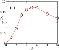
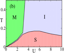
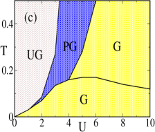
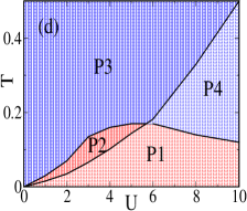
Figure 1: Colour online: (a). The transition temperature $T_{c}(U)$. (b). Superconductor-metal-insulator (S-M-I) character. The superconductor has $\rho_{dc}=0$, the M and I have $\rho_{dc}$ finite, with $d\rho_{dc}/dT>0$ for $M$ and $d\rho_{dc}/dT<0$ for $I$. (c). ‘Phases’ according to single particle DOS near Fermi level: UG is ungapped (Fermi liquid), PG is pseudo-gapped, and G is gapped. By this criteria the superconductor and $T>T_{c}$ insulator are similar. (d). Classification according to low frequency optical spectrum, i.e, the presence of the superfluid $\delta$ function, and a continuous weight extending to $\omega=0$. Both P1 and P2 are in the superfluid region but also have low frequency optical spectral weight (except at $T=0$). The distinction between P1 and P2 is quantitative, P2 has much larger low $\omega$ weight. P3 and P4 are both ‘normal’ i.e, without a superfluid peak, and also have low $\omega$ weight. Again, the P3, P4 distinction is quantitative, the low $\omega$ weight is exponentially small in P4.

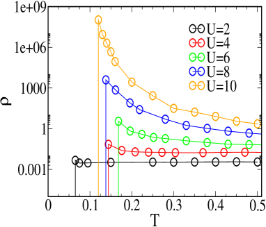
Figure 2: Colour online: The resistivity $\rho(T)$ for various interaction strengths. There is a region with $d\rho/dT<0$ above $T_{c}$ at all $U$, including the weak $U$ systems. Note that the $y$ axis spans 12 orders of magnitude.

To obtain the ground state, and in general configurations $\{|\Delta_{i}|,\theta_{i}\}$ that follow the distribution $P\{|\Delta_{i}|,\theta_{i}\}\propto e^{-\beta H_{eff}}$, we use the Metropolis algorithm to update the $|\Delta|$ and $\theta$ variables. This involves solution of the Bogoliubov-de Gennes (BdG) equation bdg for each attempted update. For equilibriation we use a ‘traveling cluster’ algorithm tca , diagonalising the BdG equation on a $8\times 8$ cluster around the update site. Global properties like pairing field correlation, DOS, etc, are computed via solution of the BdG equation on the full system. All results in this paper are for system size $32\times 32$.

If $\epsilon^{\alpha}_{n}$ are the BdG eigenvalues in some equilibrium configuration $\alpha$, the quasiparticle DOS is computed as $N(\omega)=\langle\sum_{n}\delta(\omega-\epsilon^{\alpha}_{n})\rangle$, where the angular brackets indicate averaging over $\alpha$. The quasiparticle (QP) gap is the minimum of $\epsilon^{\alpha}_{n}$ over all $\alpha,n$ at a given $T$. Similarly, the optical conductivity in an equilibrium background is formally $\sigma(\omega)=-\omega^{-1}Im(\Lambda_{xx}(q=0,\omega))$ where the current-current correlation function is defined by

$$\Lambda_{xx}(q=0,\omega)=\frac{1}{\cal{Z}}\sum_{n,m}|\langle n|j_{xx}|m\rangle|^{2}\frac{e^{-\beta E_{n}}-e^{-\beta E_{m}}}{\omega+E_{n}-E_{m}+i\delta}$$

The $|n\rangle$, $|m\rangle$ are multiparticle states of the system. We have suppressed the $\alpha$ labels above. We will discuss the simplification of this expression elsewhere. For the continuous part of $\sigma(\omega)$, i.e, excluding the superfluid response, it leads to:

$$\sigma(\omega) = \sum_{a,b}F_{1}(a,b)\frac{(n(\epsilon_{a})+n(\epsilon_{b})-1)}{\epsilon_{a}+\epsilon_{b}}\delta(\omega-\epsilon_{a}-\epsilon_{b})$$

$$~{}+\sum_{a,b}F_{2}(a,b)\frac{(n(\epsilon_{a})-n(\epsilon_{b}))}{\epsilon_{a}-\epsilon_{b}}\delta(\omega-\epsilon_{b}+\epsilon_{a})$$

where, now, the $\epsilon_{\alpha},\epsilon_{\beta}>0$, etc, are single particle eigenvalues of the BdG equations, the $n(\epsilon_{a})$, etc., are Fermi functions, and the $F$’s are current matrix elements computed from the BdG eigenfunctions. We will call the two contributions above, $\sigma_{1}(\omega)$ and $\sigma_{2}(\omega)$. The averaging of $\sigma(\omega)$ over equilibrium configurations of $\Delta_{i}$ at a given $T$ is implied. The dc resistivity $\rho={\omega_{0}}^{-1}\int_{0}^{\omega_{0}}\sigma(\omega)d\omega$, where $\omega_{0}\sim 0.1t$.

Phase diagram: Fig.1.(a) shows our result on $T_{c}(U)$, at $n=0.9$. We compute the thermally averaged pairing field correlation $S({\bf q})={1\over N^{2}}\langle\sum_{ij}|\Delta_{i}||\Delta_{j}|cos(\theta_{i}-\theta_{j})e^{i{\bf q}.{(\bf r}_{i}-{\bf r}_{j})}\rangle$ at ${\bf q}=\{0,0\}$. This is like the ‘ferromagnetic’ correlation between the $\Delta_{i}$, treating them as two dimensional moments. If the ${\bf q}=\{0,0\}$ component, $S(0)$, is ${\cal O}(1)$ it implies that the pairing field has a non-zero spatial average and would in turn induce long range order in the thermal and quantum averaged correlation $M_{ij}=\langle\langle c^{\dagger}_{i\uparrow}c^{\dagger}_{i\downarrow}c_{j\downarrow}c_{j\uparrow}\rangle\rangle$. We locate the superconducting transition from the rise in $S(0,T)$ as the system is cooled. The results are not reliable below $U/t\lesssim 1$, since $\xi$ becomes comparable to our system size, but compare very well with available QMC data for $U/t\gtrsim 2$.

Fig.1.(b) shows the basic classification of the $U-T$ space in terms of metal (M), insulator (I) and superconductor (S), the M and I regions determined from the slope $d\rho/dT$ (see Fig.2). The remarkable feature is that for $U/t\gtrsim 3$ the system is insulating, way before one can invoke a ‘hard’ gap in the spectrum due to ‘preformed pairs’. Fig.1.(c) highlights the low energy behaviour in the quasiparticle density of states (DOS). The superconducting phase has a gap for all $U$ and $T<T_{c}$. So does the large $U$ normal state, as indicated. The low $U$ system has a band like DOS for $T>T_{c}$ and the most intriguing behaviour occurs for $2\lesssim U/t\lesssim 5$, where the $T>T_{c}$ phase has a ‘dip’ in the low energy DOS, i.e, a pseudogap.

   

   

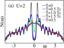
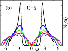
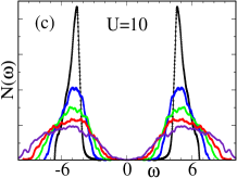
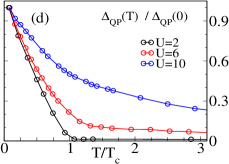
Figure 3: Colour online: Temperature dependence of the QP DOS, $N(\omega)$ at different couplings. Panels (a)-(c) have the same legends. (a). Weak coupling, $U/t=2$, (b). intermediate coupling, $U/t=6$, and (c). strong coupling, $U/t=10$. The oscillations in the DOS in panel (a) are finite size artifacts (even on a $32\times 32$ lattice). At $U/t=2$ the gap essentially vanishes at $T\sim T_{c}$, while at $U/t=6$ a small ‘hard gap’ persists to $T_{c}$ and above, although lorentzian broadening gives the impression of a pseudogap at the highest $T$. For $U/t=10$ a ‘hard gap’ persists to $T\sim 0.5$ although with a clear reduction with increasing temperature. Panel (d). shows the variation in the gap, normalised by its $T=0$ value, for the three couplings. The gap is inferred directly from the eigenvalue spectrum while the DOS has a lorentzian broadening.

Fig.1.(d) shows how the optical spectrum varies for changing $U$ and $T$. As the expression for $\sigma(\omega)$ reveals, except at $T=0$, there is in principle always low frequency spectral weight in the optical conductivity at any $U$ and $T$. This arises from thermally excited quasiparticles, and is exponentially small when $\Delta_{QP}/k_{B}T\gg 1$, i.e, broadly in the lower right part of the $U/T$ plane (the P1, P4 regions). Following the same argument, P1 and P3 have significant low frequency weight. P1 and P2 of course also have a superfluid $\delta$ function feature which P3 and P4 do not have.

Resistivity: Let us shift to the resistivity, Fig.2. From the expression for $\sigma(\omega)$ it is obvious that as long as there is a gap in the QP spectrum, the $\sigma_{1}$ term cannot contribute to the dc conductivity (it has a lower cutoff $2\Delta_{QP}$). We tried a crude model to analyse the $\rho(T)$ result. We assumed $\Delta_{i}$ configurations such that $|\Delta_{i}|$ is same at every site and is set to the $T=0$ mean field value appropriate to the $\mu$ and $U$. The phases $\theta_{i}$ are assumed to be completely random and uncorrelated between sites. Solving the BdG equations that results from these configurations, and introducing $T$ only as in the Fermi factors, leads to a result that is remarkably similar to Fig.2 for $T\gtrsim 0.3$. This suggests that the detailed $T$ dependent distributions of $|\Delta_{i}|$ and the spatial correlations in $\theta_{i}$ are not essential for a first understanding. The $\rho(T)$ for $U\gtrsim 6$ is mainly controlled by QP activation across the $T>T_{c}$ gap, while for $U\lesssim 6$ we observed a pseudogap in the spectrum generated by the toy $\{\Delta_{i}\}$ and the $\rho(T)$ behaviour is affected mainly by the scattering effect due to the random $\theta$. The M-I transition, with growing $U$ at $T>T_{c}$, is mainly due to the scattering induced by pairing (angular) disorder, rather than the opening of a clean gap in the QP spectrum.

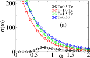
Figure 4: Colour online: Temperature dependence of the optical conductivity, $\sigma(\omega)$ in different coupling regimes. (a). For ‘weak’ coupling: $U/t=2$, the low $\omega$ region fills up rapidly and $\sigma(\omega)$ is almost $T$ independent for $T>T_{c}$. (b). For intermediate coupling, $U/t=6$, the suppressed low $\omega$ weight persists to $T\gtrsim T_{c}$, and the overall weight in the $T>T_{c}$ spectra is moderately $T$ dependent. (c). For $U/t=10$ the suppression of low $\omega$ weight persists to $T\sim 0.5$ and the integrated weight seems to increase slowly for $T>T_{c}$.

Density of states: The DOS has been investigated earlier too, and we confirm the known trends albeit with much higher resolution. Panels (a)-(c) in Fig.3 show the DOS at $U=2,~{}6,~{}10$, respectively to the left of peak, peak $T_{c}$, and right of peak, on the $T_{c}(U)$ curve. At $T=0$ all plots have the usual coherence peak at the gap edges. These diminish rapidly with $T$ and the gap begins to fill up. The fate of the gap is shown in Fig.3.(d), where $U=6$ and $10$ have a gap for $T\gg T_{c}$ (and the $U=10$ gap is strongly $T$ dependent) while the $U=2$ gap closes at $T\sim T_{c}$. This confirms that $U\sim 3$, where the M-I crossover occurs, will not have a clean gap for $T>T_{c}$.

Optics: Fig.4 shows the optical conductivity at $U=2,~{}6,~{}10$. We have not shown the $\delta$ function at $T<T_{c}$ for clarity (at $T=0$, within this calculation, the entire weight would be in the $\delta$ function). The response at $U=2$ does not have any finite $\omega$ peak but $U=6$ and $U=10$ have a $2\Delta_{QP}$ peak, arising from $\sigma_{1}(\omega)$, that show up at $T\sim 0.5T_{c}$, and grow with increasing $T$. The filling up of the low $\omega$ part is however due to thermally excited QP’s contributing via $\sigma_{2}(\omega)$. For $T>T_{c}$ the optical spectral weight weakly $T$ dependent.

In conclusion, we have studied the attractive 2D Hubbard model via a new Monte Carlo technique on large lattices. Our results on $T_{c}$ and density of states correspond to available QMC results, but our access to real frequency conductivity data allows the first determination of the metal-insulator transition in the normal state, and its relation to the single particle spectrum.

Acknowledgments: We acknowledge use of the High Performance Computing Cluster at HRI. PM acknowledges support from a DAE-SRC Outstanding Research Investigator Award, and the DST India (Athena).

References

- (1) For a recent review, see Q. Chen, J. Stajic, S. Tan and K. Levin, Phys. Repts. 412, 1 (2005).
- (2) D. M Eagles, Phys. Rev. 186, 456 (1969).
- (3) A. J. Leggett in Modern Trends in the Theory of Condensed Matter, Springer-Verlag, Berlin.
- (4) P. Nozieres and S. Schmitt-Rink, J. Low. Temp. Phys. 59, 195 (1985).
- (5) For an early review, see R. Micnas, et al., Rev. Mod. Phys. 62, 113 (1990).
- (6) M. Randeria in Bose-Einstein Condensation, Cambridge University Press (1995).
- (7) R. T. Scalettar, et al., Phys. Rev. Lett. 62, 1407 (1989).
- (8) A. Moreo and D. J. Scalapino, Phys. Rev. Lett. 66, 946 (1991).
- (9) A. Moreo, et al., Phys. Rev. B45, 7544 (1992).
- (10) M. Randeria, et al., Phys. Rev. Lett. 69, 2001 (1992).
- (11) N. Trivedi and M. Randeria, Phys. Rev. Lett. 75, 312 (1995).
- (12) B. Kyung, et al., Phys. Rev. B64, 075116 (2001).
- (13) H. Tamaki, et al., Phys. Rev. A77, 063616 (2008).
- (14) J. J. Deisz, et al., Phys. Rev. B66, 014539 (2002).
- (15) M. Keller, et al., Phys. Rev. Lett. 86, 4612 (2001).
- (16) M. Capone, et al., Phys. Rev. Lett. 88, 126403 (2002).
- (17) F. Solms, et al., Phys. Rev. B49, 15945 (1994).
- (18) Y. Dubi, et al., Nature, 449, 876 (2007).
- (19) M. Mayr, et al., Phys. Rev. Lett. 94, 217001 (2005).
- (20) V. Singh, et al., arXiv:1104.4912.
- (21) P. G. de Gennes, Superconductivity of metals and alloys, Addison Wesley (1989).
- (22) S. Kumar and P. Majumdar, Eur. Phys. J. B, 50, 571 (2006).