On the Superradiant Phase in Field-Matter Interactions

Abstract

We show that semi-classical states adapted to the symmetry of the Hamiltonian are an excellent approximation to the exact quantum solution of the ground and first excited states of the Dicke model. Their overlap to the exact quantum states is very close to $1$ except in a close vicinity of the quantum phase transition. Furthermore, they have analytic forms in terms of the model parameters and allow us to calculate analytically the expectation values of field and matter observables. Some of these differ considerably from results obtained via the standard coherent states, and by means of Holstein-Primakoff series expansion of the Dicke Hamiltonian. Comparison with exact solutions obtained numerically support our results. In particular, it is shown that the expectation values of the number of photons and of the number of excited atoms have no singularities at the phase transition. We comment on why other authors have previously found otherwise.

I Introduction

The field-matter interaction is commonly described by the Dicke Hamiltonian dicke , which considers $N$ two-level atoms with energy separation equal to $\hbar\tilde{\omega}_{A}$ immersed in an external one-mode electromagnetic field of frequency $\tilde{\omega}_{F}$ inside a cavity. This Hamiltonian comes from the standard quantization of the multipolar form of many atoms interacting with classical radiation power in the long wave approximation. The Dicke model was established exploiting the analogy with the spin. It is considered a multiatom generalization of the Jaynes–Cummings model jaynes , a completely soluble quantum Hamiltonian of a two-level atom in a one mode electromagnetic field. The Tavis–Cummings model tavis is also a many body extension of the Jaynes–Cummings model, which considers the rotating-wave approximation.

A very important feature of the Dicke Hamiltonian discovered by Hepp and Lieb hepp is the presence of a phase transition from the normal to the superradiant behaviour. The latter, introduced by Dicke to describe coherent radiation, is a collective effect involving all $N$ atoms in the sample, where the decay rate is proportional to $N^{2}$ instead of $N$, the expected result for independent atom emission. While this transition to the superradiant phase has been much debated in the literature wodk ; birula ; siva ; casta3 , due to the smallness of the field-matter coupling strength, recent experimental results indicate that it can actually be observed dimer ; baumann ; nagy .

In this contribution we use the tensorial product of $SU(2)$- and $HW(1)$-coherent states as a trial state to calculate the expectation value of the Hamiltonian and construct its energy surface. This is a function that depends on four variables $(q,p,\theta,\phi)$ which define the coherent states, and two essential parameters $(\omega_{A},\gamma)$ which are associated to the energy separation of the two-level atoms and the coupling strength between the atoms and the field, respectively. By studying the stability properties of the critical points of this energy surface we obtain the best variational wavefunction and a separatrix which divides the parameter space in two regions: normal and superradiant behaviour, according to $\gamma<\gamma_{c}$ or $\gamma>\gamma_{c}$, respectively, with $\gamma_{c}=\sqrt{\omega_{A}/4}$.

The Dicke Hamiltonian is invariant under transformations of the cyclic group $C_{2}$, a symmetry which is not preserved by the trial state. The symmetry can be restored by acting with the projectors of the symmetric and antisymmetric representations of the cyclic group $C_{2}$. We determine the statistical properties of field and matter observables in the restored variational states $|\Psi_{P}\rangle$ in the superradiant region. The comparison with the same observables evaluated from the exact diagonalization of the Hamiltonian at finite number of atoms $N$ exhibits an excellent agreement between them, which improves as $N$ becomes larger rapcom . The fidelity between both types of states is also evaluated; we establish that the fidelity in the superradiant regime is very close to unity, dropping fast in a small neighbourhood of the separatrix. The great advantage of working with the restored-symmetry states is that they allow us to write down analytic expressions for all the expectation values of field and matter observables, as well as with important mathematical relations. These analytic expressions are exact in the thermodynamic limit, when the number of particles goes to infinity.

The Dicke Hamiltonian has been studied thoroughly by Emary and Brandes emary with a variational procedure in terms of two $HW(1)$-coherent states. One of them is related to the radiation field degrees of freedom and the other arises from a Holstein-Primakoff (H-P) realization of the $SU(2)$ generators holstein . They obtain the appropriate relation between the parameters of the Dicke Hamiltonian to describe the phase transition, as well as a description for the normal phase in the thermodynamic limit. However, they consider in the superradiant region, an approximated Dicke Hamiltonian coming from a series expansion of the H-P realization truncated to second order in terms of the ratio between the number of excited atoms over the total number of atoms, assuming that is a very small quantity. Under this assumption Nagy et al. nagy found singularities at $\gamma=\gamma_{c}$ in the expectation values of the number of photons and the number of excited atoms, and related them with the divergences in their corresponding fluctuations emary .

In this contribution we extend and provide details of the calculations presented in rapcom . The expectation values of the mentioned observables are calculated by means of the symmetry adapted variational states and find that there is in fact a divergence of the expectation values, but that this remains throughout the superradiant region, contrary to the published results: there is no singularity. The expectation value of the number of photons $\langle\hat{a}^{\dagger}\hat{a}\rangle$ and the squared fluctuation of the first quadrature of the electromagnetic field $(\Delta\hat{q})^{2}$ are proportional to the number of atoms at the phase transition and in the superradiant regime, while the squared fluctuation $(\Delta\hat{J}_{x})^{2}$ is proportional to $N^{2}$ in the same region. Comparison with the exact numerical solution supports our results. This could have consequences in studies of entanglement and chaos in the superradiant region.

II Dicke Hamiltonian and Symmetry Adapted States

The Dicke Hamiltonian involves the collective interaction of $N$ two-level atoms with energy separation $\hbar\tilde{\omega}_{A}$ with a one-mode radiation field of frequency $\tilde{\omega}_{F}$ in the long wavelenght limit. It has the form

$$H_{D}=\hat{a}^{\dagger}\hat{a}+\omega_{A}\hat{J}_{z}+\frac{\gamma}{\sqrt{N}}\left(\hat{a}^{\dagger}+\hat{a}\right)\left(\hat{J}_{+}+\hat{J}_{-}\right)\ ,$$ (1)

where $\omega_{A}\equiv\tilde{\omega}_{A}/\tilde{\omega}_{F}$ is given in units of the frequency of the field, and $\gamma=\tilde{\gamma}/\tilde{\omega}_{F}=\sqrt{(2\pi\varrho/\hbar\,\tilde{\omega}_{F})}\,\vec{d}_{ba}\cdot\vec{e}_{P}$, is the coupling parameter between the matter and field. The $\varrho$ denotes the density of atoms in the quantization volume, $\vec{d}_{ba}$ is the excitation matrix element of the electric dipole operator of a single atom, and $\vec{e}_{P}$ the polarization vector. The operators $\hat{a}^{\dagger},\,\hat{a}$ denote the one-mode creation and annihilation photon operators; $\hat{J}_{z}$ the atomic relative population operator; and $\hat{J}_{\pm}$ the atomic transition operators. We will consider completely symmetric states for which we have $N=2\,j$.

Later we will find it convenient to divide the Dicke Hamiltonian by the total number of particles, having in this way an intensive Hamiltonian operator. In order to study the thermodynamic limit one would take $N\rightarrow\infty$.

To find the symmetries of the Hamiltonian, one considers the unitary transformation $\hat{U}=\exp\left(i\phi_{0}\hat{\Lambda}\right)$ with $\hat{\Lambda}=\hat{a}^{\dagger}\hat{a}+\hat{J}_{z}+\sqrt{\hat{\vec{J}}^{2}+1/4}-1/2$ denoting the excitation number operator. One can show that

$$\hat{U}\,\hat{a}\,\hat{U}^{\dagger}=e^{-i\phi_{0}}\,\hat{a}\ ,\qquad\hat{U}\,\hat{J}_{+}\,\hat{U}^{\dagger}=e^{-i\phi_{0}}\,\hat{J}_{+}\ ,$$ (2)

with the corresponding hermitean conjugated relations. Substituting these results into the expression for the Dicke Hamiltonian one has

$$\hat{U}\,H_{D}\,\hat{U}^{\dagger}=\hat{a}^{\dagger}\hat{a}+\omega_{A}\hat{J}_{z}+\frac{\gamma}{\sqrt{N}}\left(\hat{a}^{\dagger}\,\hat{J}_{-}+\hat{a}\,\hat{J}_{+}\right)+\frac{\gamma}{\sqrt{N}}\left(e^{-2i\phi_{0}}\,\hat{a}^{\dagger}\,\hat{J}_{+}+e^{2i\phi_{0}}\,\hat{a}\,\hat{J}_{-}\right)\ .$$ (3)

If the counter-rotating term (last term of the expression) is neglected, one recovers the Tavis-Cummings model and it is immediate that it is invariant under any rotation with arbitrary $\phi_{0}$. Their symmetrized solutions have been thoroughly studied in ocasta1 ; ocasta2 . For the Dicke Hamiltonian, it is necessary to restrict to rotations by an angle $\phi_{0}=0,\,\pi$ for the Hamiltonian to remain invariant. Thus the invariance group for the Dicke model is ${\cal C}_{2}=\left\{I,\,\hbox{\normalsize e}^{i\,\pi\,\hat{\Lambda}}\right\}$.

The projection operators for this group are

$$\hat{P}_{\pm}=\frac{1}{2}\left(I\pm\hbox{\normalsize e}^{i\,\pi\,\hat{\Lambda}}\right)\ ,$$ (4)

which allow us to write the eigenfunctions of the Hamiltonian displaying its symmetry explicitly. In terms of the eigenstates $|\nu\rangle$ of the photon number operator, and the square of the angular momentum and its projection in the z-axis $|j,\,m\rangle$, they may be expressed as

$$|\phi^{k}_{j;\pm}\rangle=\sum_{\lambda=0}^{\infty}\ \sum_{\nu=\max\{0,\lambda-2j\}}^{\lambda}\tfrac{\left(1\pm(-1)^{\lambda}\right)}{2}\ c^{k}_{\lambda,\,\nu}\ |\nu\rangle\otimes|j,\,\lambda-j-\nu\rangle\ ,$$ (5)

where $|\phi^{k}_{j;+}\rangle$ contains only even values of $\lambda=\nu+j+m$, the eigenvalues of $\hat{\Lambda}$, while $|\phi^{k}_{j;-}\rangle$ contains the odd ones. The index $k$ denotes the state number of the even and odd solutions. In practice one uses a maximum value for $\lambda$ which guaranteed the convergence in the energy eigenvalues of the ground and first excited states. The coefficients $c^{k}_{\lambda,\,\nu}$ can be obtained from the diagonalization of the Hamiltonian matrix, whose dimension is

$$d=\left\{\begin{array}[]{r@{\quad,\qquad}l}\frac{1}{2}\left(\lambda_{\max}+1\right)\left(\lambda_{\max}+2\right)&\lambda_{\max}\leq 2j\ ;\\ \left(2j+1\right)\left(\lambda_{\max}-j+1\right)&\lambda_{\max}\geq 2j\ ,\end{array}\right.$$

in the basis states without definite parity of $\lambda$. This matrix, in the symmetry adapted basis states, breaks into two pieces of even and odd parity respectively. For $\lambda\geq 2j$, the dimensions of the matrices are

$$d_{+}=(j+1)^{2}+(2j+1)(s_{+}-j)\,,\quad d_{-}=j(j+1)+(2j+1)(s_{-}-j)\,,$$

for integer $j$, with $s_{+}=\lfloor\lambda_{max}/2\rfloor$ and $s_{-}=\lfloor(\lambda_{max}+1)/2\rfloor$. For $\lambda<2j$, they are $d_{+}=(s_{+}+1)^{2}$ and $d_{-}=s_{-}(s_{-}+1)$. Similar expressions can be obtained for half integer $j$.

III Energy Surface and Critical Points

The energy surface is found by taking the expectation value of the Dicke Hamiltonian with respect to the tensorial product of coherent states of Heisenberg–Weyl and $SU(2)$ groups $|\alpha\rangle\otimes|\zeta\rangle\$, given by hecht ; gilmore1972

$$|\alpha\rangle = \exp\left(-\left|\alpha\right|^{2}/2\right)\,\sum_{\nu=0}^{\infty}\frac{\alpha^{\nu}}{\sqrt{\nu!}}\,|\nu\rangle\ ,$$

$$|\zeta\rangle = \frac{1}{\left(1+\left|\zeta\right|^{2}\right)^{j}}\,\sum_{m=-j}^{j}\binom{2j}{j+m}^{1/2}\,\zeta^{j+m}\,|j,\,m\rangle\ ,$$

where the parameters $\alpha$ and $\zeta$ are complex numbers. Using the Ritz variational principle one may find the best variational approximation to the ground state energy of the system and its corresponding eigenstate.

To calculate the expectation values of the field and matter observables it is convenient to find the representation of the angular momentum and Weyl generators with respect to the tensorial product $|\alpha\rangle\otimes|\zeta\rangle\$ hecht . For example, for the annihilation photon operator we consider the matrix element

$$\langle\alpha|\hat{a}|\psi\rangle = \hbox{\normalsize e}^{-\tfrac{|\alpha|^{2}}{2}}\,\langle 0|\hbox{\normalsize e}^{\alpha^{*}\,\hat{a}}\ \hat{a}|\psi\rangle$$ (6)

$$= \left(\frac{\partial\ \ }{\partial\alpha^{*}}+\frac{\alpha}{2}\right)\,\langle\alpha|\psi\rangle\ ,$$

where $|\psi\rangle$ denotes an arbitrary state. We proceed in a similar form for the other observables. The representations of the annihilation and creation photon operators are thus given by

$$\hat{a}\rightarrow\frac{\partial\ \ }{\partial\alpha^{*}}+\frac{\alpha}{2}\,,\quad\hat{a}^{\dagger}\rightarrow\alpha^{*}\,,$$

and for the matter observables we have

$$\hat{J}_{z} \rightarrow -\frac{j}{1+|\zeta|^{2}}+\zeta^{*}\,\frac{\partial\ \ }{\partial\zeta^{*}}\,,$$

$$\hat{J}_{+} \rightarrow j\,\zeta^{*}\frac{2+|\zeta|^{2}}{1+|\zeta|^{2}}+(\zeta^{*})^{2}\,\frac{\partial\ \ }{\partial\zeta^{*}}\,,$$

$$\hat{J}_{-} \rightarrow \frac{j\,\zeta}{1+|\zeta|^{2}}+\frac{\partial\ \ }{\partial\zeta^{*}}\,.$$

The energy surface can be then calculated straightforwardly ocasta1 ; ocasta2

$${\cal H}(\alpha,\,\zeta) \equiv \langle\alpha|\otimes\langle\zeta|H_{D}|\alpha\rangle\otimes|\zeta\rangle$$ (7)

$$= \frac{1}{2}\left(p^{2}+q^{2}\right)-j\,\omega_{A}\,\cos\theta+2\sqrt{j}\gamma\,q\,\sin\theta\,\cos\phi\ .$$

In this expression we take the harmonic oscillator realization for the field part and the stereographic projection for the angular momentum part,

$$\alpha=\frac{1}{\sqrt{2}}\left(q+i\,p\right)\ ,\qquad\zeta=\hbox{\normalsize e}^{-i\,\phi}\,\tan\frac{\theta}{2}\ ,$$ (8)

where $(q,p)$ correspond to the expectation values of the quadratures of the field, and $(\theta,\phi)$ determine a point on the Bloch sphere.

The minima and degenerate critical points are obtained by means of the catastrophe formalism gilmore3 . By calculating the Hessian of the energy surface, we see that when $\gamma_{c}^{2}=\omega_{A}/4$ the critical points degenerate and, for that value of the field-matter coupling, the phase transition from the normal to the superradiant behaviour of the atoms takes place.

The critical points which minimize ${\cal H}$ are given by

$$\begin{array}[]{lllll}\theta_{c}=0\,,&q_{c}=0\,,&p_{c}=0\,,&\hbox{ for }|\gamma|<\gamma_{c}\,,\\ \theta_{c}=\arccos(\gamma_{c}/\gamma)^{2}\,,&q_{c}=-2\,\sqrt{j}\,\gamma\,\sqrt{1-(\gamma_{c}/\gamma)^{4}}\cos{\phi_{c}}\,,&p_{c}=0\,,&\hbox{ for }|\gamma|>\gamma_{c}\ .\end{array}$$ (9)

The last column of this array shows the conditions in parameter space to guarantee that they constitute a minimum of the energy surface. The first row describes the minimum critical points for the normal phase, while the second row describes those for the superradiant regime. In this last case one has $\phi_{c}=0,\,\pi$. (If one were to consider a case in which $\omega_{A}<0$, we would then have $\gamma_{c}^{2}=-\omega_{A}/4$ and the critical points for the normal phase would be $\theta_{c}=\pi,\ q_{c}=0,\ p_{c}=0$, for $|\gamma|<\gamma_{c}$). It is convenient to work with the variable $x=\gamma/\gamma_{c}$ in terms of which the energy values for the minima just described are

$$E_{\hbox{normal}}=-2N\,\gamma_{c}^{2}\ ,\quad E_{\hbox{superradiant}}=-N\,\gamma_{c}^{2}\,x^{2}\,\left(1+x^{-4}\right)\ .$$ (10)

In a similar form, the expectation values of $\hat{\Lambda}$ at the minima are

$$\lambda_{\hbox{normal}}=0\,,\quad\lambda_{\hbox{superradiant}}=\tfrac{N}{2}\,\left[1-x^{-2}+2\,\gamma_{c}^{2}\,x^{2}\,\left(1-x^{-4}\right)\right]\ .$$ (11)

The fluctuations $\Delta\hat{\Lambda}$ are zero in the normal region, and in the superradiant phase take the form

$$\Delta\hat{\Lambda}=\sqrt{\tfrac{N}{2}\left(\tfrac{1}{2}+2\,\gamma^{2}_{c}\,x^{2}\right)\left(1-x^{-4}\right)}\ .$$ (12)

To study the statistical properties of the variational states in the superradiant regime we calculate the expectation values of linear matter and field observables with respect to the tensorial product of coherent states, as well as their fluctuations. The results are given in the left side of Table 1. Notice that we have introduced the quadratures operators $\hat{q}$ and $\hat{p}$ of the electromagnetic field and they can be written in terms of the creation and annihilation photon operators.

IV Symmetry-Adapted Coherent States

To build variational states which preserve the symmetry of the Dicke Hamiltonian we apply the projectors of even and odd parity (4) to the coherent states $|\alpha\rangle\otimes|\zeta\rangle$, to obtain

$$|\alpha,\,\zeta\rangle_{\pm}={\cal N}_{\pm}\Big{(}|\alpha\rangle\otimes|\zeta\rangle\pm\ |-\alpha\rangle\otimes|-\zeta\rangle\Big{)}\ ,$$ (13)

where the normalization factors ${\cal N}_{\pm}$ are given by

$${\cal N}_{\pm}^{-2}=2\,\left(1\pm\exp\left(-2\,|\alpha|^{2}\right)\left(\frac{1-|\zeta|^{2}}{1+|\zeta|^{2}}\right)^{N}\right)\ .$$ (14)

The expression (13) is useful because it allows us to calculate the expectation values of the relevant operators in closed form, in particular the expectation value of the Hamiltonian. Evaluating the energy surface with respect to the symmetry adapted states, one obtains

$$\langle H\rangle_{\pm} = \pm\frac{1}{2}\left(p^{2}+q^{2}\right)\left\{1-\frac{2}{1\pm e^{\pm(p^{2}+q^{2})}(\cos\theta)^{\mp N}}\right\}$$ (15)

$$- \frac{N}{2}\,\omega_{A}\left\{(\cos\theta)^{\pm 1}\pm\frac{\tan^{2}\theta\,\cos\theta}{1\pm e^{\pm(p^{2}+q^{2})}(\cos\theta)^{\mp N}}\right\}$$

$$+ \sqrt{2\,N}\,\gamma\left\{\frac{\pm p\,\tan\theta\,\sin\phi+q\,e^{p^{2}+q^{2}}\sin\theta\,\cos\phi\,(\cos\theta)^{-N}}{e^{p^{2}+q^{2}}(\cos\theta)^{-N}\pm 1}\right\}\,.$$

In the limit $N\rightarrow\infty$, $\langle H\rangle_{+}$ reduces to Eq.(7), when $|\cos\theta|\neq 1$. However, it is important to stress that the analysis can be carried out for any value of $N$, and in this contribution we work at finite $N$.

The traditional approach in many-body physics is to use the critical points in Eq.(9) of the original energy surface, in order to obtain the trial state which approximates the two lowest energy states, and in which to evaluate the expectation values of the observables. Formally, one should calculate the critical points of (15), instead of that, we use the critical points associated to Eq.(7). However all of their critical points also are extreme values for (15), except in a small vicinity of the separatrix, as shown in Fig.(1). In that figure, the derivatives of the energy surface, given in (15), with respect to $q$ and $\theta$, evaluated at the critical points $q_{c}$ and $\theta_{c}$, are plotted against $\gamma$. (The derivatives with respect to the other two variables, $p$ and $\phi$, are identically zero). The neighborhood around the separatrix, where they differ, diminishes as $j$ increases (cf. Fig.(2)). For the superradiant region in which the points are critical , they are also minima. The stability analysis of the energy surface (15) and the study of their behaviour in the near-neighborhood of the separatrix will be reported elsewhere castanos2011_03 .

By substituting the critical points $p_{c}=0$, $q_{c}=-2\,\sqrt{j}\,\gamma_{c}\,x\,\sqrt{1-x^{-4}}\,\cos\phi_{c}$, and $\cos\theta_{c}=x^{-2}$ in (15), the energy surface associated to the superradiant regime takes the form

$$\langle H\rangle_{\pm}=-N\gamma_{c}^{2}x^{2}\,\left[2-(1-x^{-4})\,\frac{1\mp F}{1\pm F}\right]\ ,$$ (16)

where we have defined

$$x=\gamma/\gamma_{c}\ ,\qquad F=x^{-2N}\,\hbox{\normalsize e}^{-2N\,\gamma_{c}^{2}\,x^{2}\left(1-x^{-4}\right)}\ .$$ (17)

The overlap between the ordinary coherent states and our symmetry-adapted states can be written as

$$|\langle\alpha_{c}\,\zeta_{c}\,|\,\alpha_{c}\,\zeta_{c}\rangle_{\pm}\,|^{2}=\frac{1}{2}\,(1\pm F)\ .$$ (18)

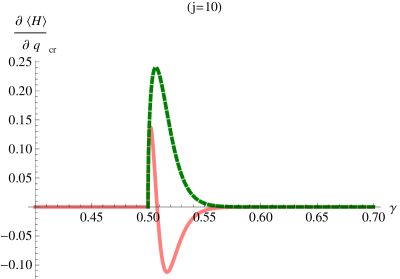
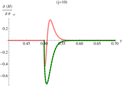
Figure 1: Derivatives of the energy surface of the symmetry-adapted states, evaluated at the critical points $q_{c}$ and $\theta_{c}$, are plotted as a function of the interaction strength $\gamma$. We use the frequency $\omega_{A}=1$ and $N=20$ atoms. Continuous lines refer to the ground state while dashed lines to the first excited state.

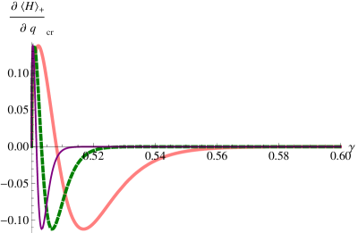
Figure 2: Derivative of the energy surface of the adapted-symmetry states, calculated at $q_{c}$ and $\theta_{c}$, is displayed as a function of the interaction strength $\gamma$, for different number of atoms. The plots correspond to $N=20,\,50,\,100$ atoms. It can be seen that the neighborhood of discrepancy from zero diminishes as $N$ increases. In all cases $\omega_{A}=1$.

In Fig. (3) the energy surfaces for the even and odd parities of $\lambda$ are shown together with those for the exact solution, showing a remarkable agreement between them in spite of having considered a small number of atoms $N=20$. For the odd parity case, we have proposed, in the normal region ($|\gamma|<\gamma_{c}$), a combination of states with $\lambda=1$:

$$|\phi_{1}\rangle=\cos\Omega\,|0\rangle\otimes|j,\,-j+1\rangle-\frac{\gamma}{|\gamma|}\,\sin\Omega\,|1\rangle\otimes|j,\,-j\rangle\ ,$$ (19)

and minimized the expectation value of the Hamiltonian with respect to $\Omega$. One finds $\tan(2\,\Omega_{c})=2\,|\gamma|/(1-\omega_{A})$. This gives, for the resonant case, $\Omega_{c}=\pi/4$.

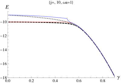
Figure 3: Energies of the ground and first excited states of the Dicke Hamiltonian as a function of the interaction strength $\gamma$, for the frequency $\omega_{A}=1$ and $N=20$ atoms. The thin and thick continuous lines show the ground and first excited energies, respectively, evaluated with the projected variational states, while the dashed and dotted lines correspond to the ground and first excited energies calculated through the diagonalization of the matrix Hamiltonian.

V Statistical Properties

V.1 Expectation values

One can calculate the expectation values of the matter and field main operators in the superradiant regime with respect to the symmetry adapted states. The results are collected in Table 1 together with those associated to the coherent states. Both are evaluated at the critical points for the energy surface, and are given in terms of $x$ and $F$.

Table 1: Expectation values and fluctuations of matter and field observables for the coherent and symmetry-adapted states in the superradiant regime. The mean-field behaviour obtained in the normal region can be recovered by taking the limit $x\rightarrow 1$.

	Coherent	Symmetry Adapted
$\langle\hat{q}\rangle$	$-\sqrt{2N}\,\gamma_{c}\,x\,\sqrt{1-x^{-4}}$	$0$
$\langle\hat{p}\rangle$	$0$	$0$
$\langle\hat{J}_{x}\rangle$	$\frac{N}{2}\,\sqrt{1-x^{-4}}$	$0$
$\langle\hat{J}_{y}\rangle$	$0$	$0$
$\langle\hat{J}_{z}\rangle$	$-\frac{N}{2}\,x^{-2}$	$-\frac{N}{2}\,x^{2}\left(1-\frac{1-x^{-4}}{1\pm F}\right)$
$\langle\hat{a}^{\dagger}\hat{a}\rangle$	$N\,\gamma_{c}^{2}\,x^{2}\,\left(1-x^{-4}\right)$	$N\,\gamma_{c}^{2}\,x^{2}\,\left(1-x^{-4}\right)\left(\frac{1\mp F}{1\pm F}\right)$
$\langle\hat{\Lambda}\rangle$	$\frac{N}{2}\left(1-x^{-2}+2\,\gamma_{c}^{2}\,x^{2}\,\left(1-x^{-4}\right)\right)$	$\frac{N}{2}\left(\frac{1-x^{-2}}{1\pm F}\right)\Big{\{}x^{2}+2\,\gamma_{c}^{2}\,x^{2}\,\left(1+x^{2}\right)$ pittsburg
		$\phantom{pittsburgh}\mp\left(x^{4}+2\,\gamma_{c}^{2}\,x^{2}\,\left(1+x^{2}\right)\right)\,F\Big{\}}$
$\mathbf{(\Delta\hat{q})^{2}}$	$\frac{1}{2}$	$\frac{1}{2}+2N\,\gamma_{c}^{2}\,x^{2}\,\left(\frac{1-x^{-4}}{1\pm F}\right)$
$(\Delta\hat{p})^{2}$	$\frac{1}{2}$	$\frac{1}{2}\mp 2N\,\gamma_{c}^{2}\,x^{2}\,\left(\frac{1-x^{-4}}{1\pm F}\right)\,F$
$\mathbf{(\Delta\hat{J}_{x})^{2}}$	$\frac{N}{4}\,x^{-4}$	$\frac{N}{4}\left(1+\frac{\left(N-1\right)\left(1-x^{-4}\right)}{1\pm F}\right)$
$(\Delta\hat{J}_{y})^{2}$	$\frac{N}{4}$	$\frac{N}{4}\left(1\pm\frac{\left(N-1\right)\left(1-x^{4}\right)F}{1\pm F}\right)$
$(\Delta\hat{J}_{z})^{2}$	$\frac{N}{4}\,\left(1-x^{-4}\right)$	$\frac{N}{4}\,\frac{\left(1-x^{-4}\right)}{\left(1\pm F\right)^{2}}\,\left[1\mp\left(N-1\right)\left(1-x^{4}\right)\,F-x^{4}F^{2}\right]$
$(\Delta\,\hat{a}^{\dagger}\hat{a})^{2}$	$N\,\gamma_{c}^{2}\,x^{2}\,\left(1-x^{-4}\right)$	$N\,\gamma_{c}^{2}\,x^{2}\,\bigg{\{}N\,\gamma_{c}^{2}\,x^{-6}\,\left(1-x^{4}\right)\left(\frac{1\mp F}{1\pm F}\right)^{2}$luisoctaviosfmal
		$+\left(1-x^{-4}\right)\left[N\,\gamma_{c}^{2}\,x^{2}\,\left(1-x^{-4}\right)+\frac{1\mp F}{1\pm F}\right]\bigg{\}}$
$\langle\hat{J}_{z}\,\hat{a}^{\dagger}\hat{a}\rangle$	$-N\,\gamma_{c}^{2}\,\left(1-x^{-4}\right)$	$-N\,\gamma_{c}^{2}\,x^{4}\left(1-x^{-4}\right)\left(\frac{x^{-4}\mp F}{1\pm F}\right)$
$\langle\hat{J}_{x}\,\hat{q}\rangle\rangle$	$-\sqrt{\frac{N^{3}}{2}}\,\gamma_{c}\,x\,\left(1-x^{-4}\right)$	$-\sqrt{\frac{N^{3}}{2}}\,\gamma_{c}\,x\,\frac{1-x^{-4}}{1\pm F}$

Observe that, for expectation values different from zero in the symmetry adapted states, the coherent state results can be obtained from the former by letting $F$ go to zero, with the exception of $(\Delta\hat{q})^{2}$ and $(\Delta\hat{J}_{x})^{2}$. These two exceptions arise because $\langle\hat{q}\rangle=\langle\hat{J}_{x}\rangle=0$ for the former but not for the latter. That $F$ tends very quickly to zero as a function of $\gamma$ (or $x$) can be seen in Fig. (4), especially for large $N$. This is why coherent states have been so successful in the past as trial functions. It can be seen that the quantities which differ the most are some fluctuations of matter and field observables. To assess this difference we evaluated the fluctuation of the atomic transition operator $\hat{J}_{x}$ and of the first quadrature of the electromagnetic field, $\hat{q}$.

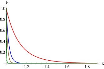
Figure 4: The behavior of $F$ as a function of $x$ is presented for a number of atoms in the cavity equal to $N=2,10,20$ and $100$. We use $\gamma_{c}=0.5$ (in resonance).

V.2 Fluctuations $\Delta\hat{J}_{x}$ and $\Delta\hat{q}$

In Fig. (5) we show the fluctuation of the transition operator $(\Delta\hat{J}_{x})^{2}$ for the ground and first excited states of the Dicke model with $N=10$ atoms and $\omega_{A}=1$, calculated for the symmetry adapted states and the coherent states. While $(\Delta\hat{J}_{x})^{2}/N^{2}$ tends erroneously to zero for the coherent state, as $x$ increases, the results for the symmetry-adapted states show the appropriate quadratic dependence in $N$, asymptotically reaching $(\Delta\hat{J}_{x})^{2}\approx N^{2}/4$. In Fig. (6) we show $(\Delta\hat{q})^{2}$ for the ground and first excited states of the Dicke model with $N=10$ atoms and $\omega_{A}=1$ calculated for the symmetry-adapted states and the coherent states. While for the coherent state the result is a constant $1/2$, for the symmetry adapted states one has a linear dependence in the number of atoms. Additionally, in both cases one can see that the symmetry-adapted states compare really well with the exact result obtained from the diagonalization of Hamiltonian for the even and odd parity states, except in the close vicinity of the separatrix of the physical system rapcom . These results show clearly the benefit of using the symmetry-adapted states over the coherent ones.

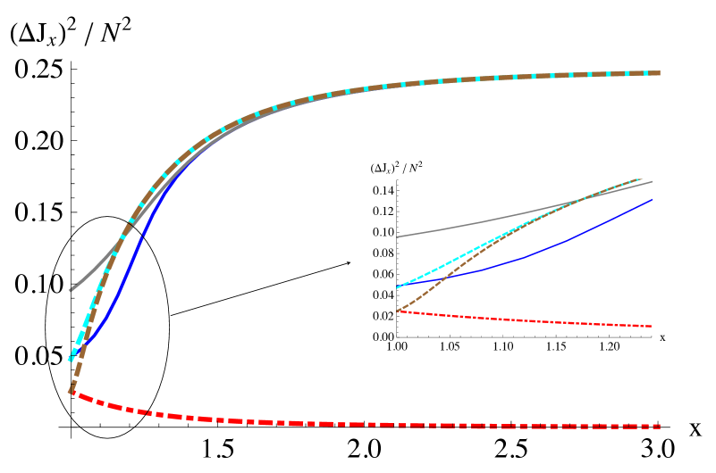
Figure 5: Fluctuation of the atomic transition operator $\hat{J}_{x}$ evaluated for the ground and first excited states of the Dicke Hamiltonian as a function of the interaction strength $\gamma$, for the frequency $\omega_{A}=1$ and $N=10$ atoms. The dashed dark and light lines show the fluctuations for the ground and first excited states, respectively, evaluated with the projected variational states, while the continuous lines describe the correspodning fluctuations calculated through the diagonalization of the matrix Hamiltonian. The result for the coherent state is shown in the dashed-dotted line.(Color online.)

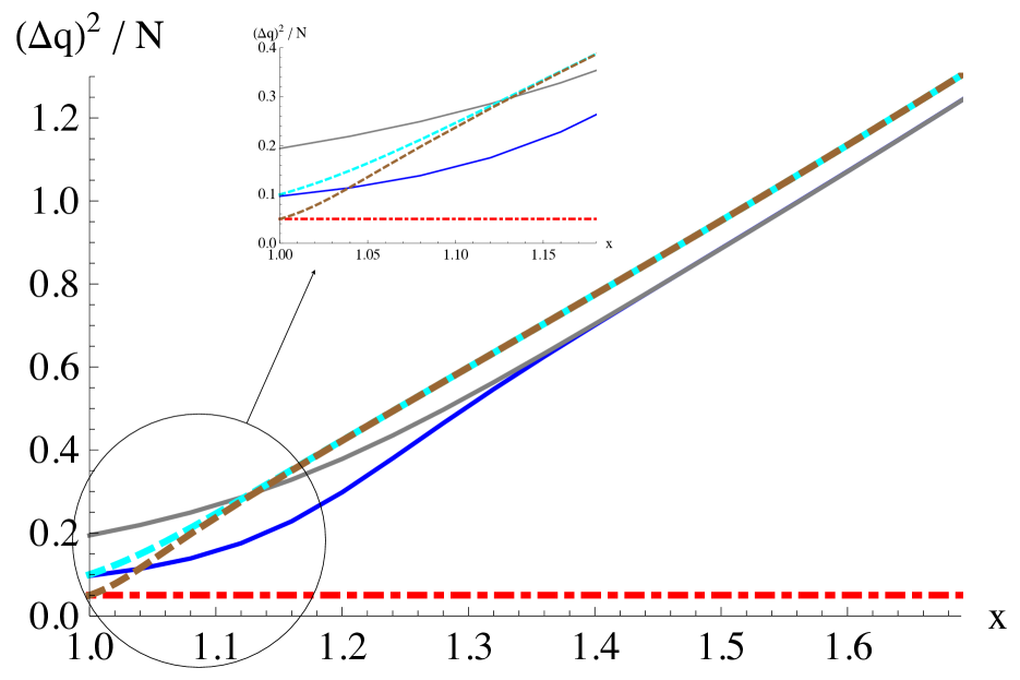
Figure 6: Fluctuation of the electromagnetic field first quadrature operator $\hat{q}$ evaluated for the ground and first excited states of the Dicke Hamiltonian as a function of the interaction strength $\gamma$, for the frequency $\omega_{A}=1$ and $N=10$ atoms. The dashed dark and light lines show the fluctuations of the ground and first excited states, respectively, evaluated with the projected variational states, while the continuous lines display the fluctuations of the ground and first excited states calculated through the diagonalization of the matrix Hamiltonian. The result for the coherent state is shown in the dashed-dotted line.(Color online.)

V.3 Joint probability distribution function

The joint probability of finding $\nu$ photons and $n_{e}=j+m$ excited atoms, for even and odd parity states, is obtained by taking the modulus square of the scalar product of the Fock and angular momentum states $|\nu\rangle\otimes|N,\,n_{e}\rangle$ with the symmetry-adapted states. The result depends on the values of $N$, $\gamma_{c}$, and $x$, and it is given by

$${\cal P}_{\pm}(\nu,\,n_{e}) = \left[1\pm\left(-1\right)^{\nu+n_{e}}\right]\,\frac{1}{\nu!}\left[N\,\gamma_{c}^{2}\,x^{2}\,\left(1-x^{-4}\right)\right]^{\nu}$$ (20)

$$\times\binom{N}{n_{e}}\left(\frac{1-x^{-2}}{2}\right)^{n_{e}}\left(\frac{1+x^{-2}}{2}\right)^{N-n_{e}}\,x^{N}\,\frac{\sqrt{F}}{1\pm F}\ .$$

The joint probability distribution functions, for the even- and odd-parity states, are shown in Figs. (7, 8) for a system of $N=10$ atoms and in resonance, i.e., $\omega_{A}=1$. In Fig. (7), we consider $\gamma=0.55$ and in Fig. (8), $\gamma=1.0$. It is clear that there are holes in the distributions of each plot, corresponding to the forbidden values (odd or even) of the sum $\nu+n_{e}$. Note that the Poissonian distribution when near the separatrix ($\gamma=0.55$) turns into a quasi-normal distribution as we move away ($\gamma=1$). While very few photons and excited atoms contribute to the state in the first case, many more contribute in the second case, as is to be expected.

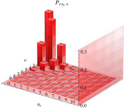
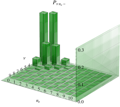
Figure 7: The joint probability distribution function of photons and excited atoms is shown, for $\gamma_{c}=0.5$, $\gamma=0.55$, and $N=10$ atoms. At the left, we plot the result for the even parity states while at the right we indicate the distribution for the odd ones.

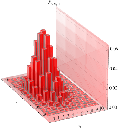
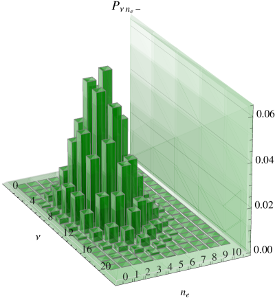
Figure 8: The joint probability distribution function of photons and excited atoms is shown, for $\gamma_{c}=0.5$, $\gamma=1.0$, and $N=10$ atoms. At the left, we plot the result for the even parity states while at the right we indicate the distribution for the odd ones.

By summing over the number of photons $\nu$ or the excited atoms $n_{e}$, one determines the corresponding marginal distributions. For the distribution of the number of photons one has

$${\cal P}_{\pm}(\nu)=\frac{1}{\nu!}\left[N\,\gamma_{c}^{2}\,x^{2}\,\left(1-x^{-4}\right)\right]^{\nu}\,\left[x^{N}\pm\left(-1\right)^{\nu}x^{-N}\right]\,\frac{\sqrt{F}}{1\pm F}\ ,$$ (21)

while for the distribution of the number of excited atoms the result is

$${\cal P}_{\pm}(n_{e})=\binom{N}{n_{e}}\,\left(\frac{1-x^{-2}}{2}\right)^{n_{e}}\,\left(\frac{1+x^{-2}}{2}\right)^{N-n_{e}}\,\frac{1\pm\left(-1\right)^{n_{e}}x^{2N}F}{1\pm F}\ .$$ (22)

The behavior of these probability distribution functions for even and odd parity states is shown in Figs. (9) and  (10) for values of $\gamma$ close to ($x=1.1$) and far from ($x=2.0$ ) the separatrix. For $x=1.1$, they are different, while for $x=2$, they cannot be distinguished. We notice that the binomial and Poissonian distributions become quasi-normal as we move away from the separatrix. This is to be expected, since, from the results given in Table 1, it is immediate that the distribution function of photons, Eq. (21), can be rewritten as

$${\cal P}_{\pm}(\nu) = \frac{1}{\nu!}\mu^{\nu}\hbox{\normalsize e}^{-\mu}\left[\frac{1\pm(-1)^{\nu}x^{-2N}}{1\pm\hbox{\normalsize e}^{-2\mu}x^{-2N}}\right]\ ,$$ (23)

where $\mu=\langle\hat{a}^{\dagger}\hat{a}\rangle$ is the expectation value of the photon number operator in the coherent state. For large values of $N$ this distribution becomes a Poisson distribution, which in this limit is equivalent to the normal distribution

$${\cal P}_{\pm}(\nu) \approx \frac{1}{\sqrt{2\pi\mu}}\exp\left[-\frac{\left(\nu-\mu\right)^{2}}{2\mu}\right]\ .$$ (24)

In Fig. (9), the distribution of the number of excited atoms for the even- and odd-parity states are shown. For $x=1.1$, close to the separatrix, they are different, while for $x=2$, we can not distinguish them.

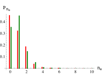
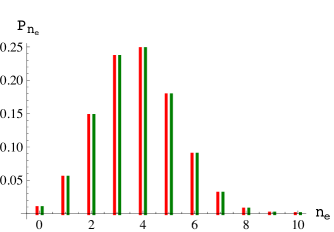
Figure 9: The probability distribution of excited atoms is shown, for $\gamma_{c}=0.5$ and $N=10$ atoms. At left we plot the result for $\gamma=0.55$, while at the right for $\gamma=1$. In both cases the red bar (left) indicates the distribution of the even parity states and the green bar (right) the result for the odd ones.

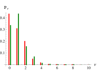
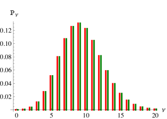
Figure 10: The probability distribution of photons is shown, for $\gamma_{c}=0.5$ and $N=10$ atoms. At left we plot the result for $\gamma=0.55$, while at the right for $\gamma=1$. In both cases the red bar (left) indicates the distribution of the even parity states and the green bar (right) the result for the odd ones.

For the distribution function of the excited number of atoms, in the limit when $N\gg 1$ one has

$${\cal P}_{\pm}(n_{e}) \approx \frac{1}{\sqrt{\pi\left(1-x^{-4}\right)N/2}}\exp\left[-\frac{\left(n_{e}-\left(1-x^{-2}\right)N/2\right)^{2}}{\left(1-x^{-4}\right)N/2}\right]\ ,$$ (25)

which for large values of $x$ also gives a normal distribution:

$${\cal P}_{\pm}(n_{e}) \approx \frac{1}{\sqrt{\pi N/2}}\exp\left[-\frac{\left(n_{e}-N/2\right)^{2}}{N/2}\right]\ .$$ (26)

VI Projected States vs. Exact Solution

By substituting the critical points of the superradiant phase into the symmetry adapted variational states (13, 14), we obtain

$$|\alpha_{sr},\zeta_{sr}\rangle_{\pm} = \frac{\pm 1}{\sqrt{2^{N+1}\left(1\pm F\right)}}\,\exp\left[-\tfrac{N}{2}\gamma_{c}^{2}\,x^{2}\,\left(1-x^{-4}\right)\right]\,\sum_{\nu,\,n_{e}}\left(1\pm(-1)^{\nu+n_{e}}\right)\,\frac{\left(\sqrt{N}\,\gamma_{c}\,x\right)^{\nu}}{\sqrt{\nu!}}\,$$ (27)

$$\times \binom{N}{n_{e}}^{1/2}\,\left(1-x^{-2}\right)^{(\nu+n_{e})/2}\,\left(1+x^{-2}\right)^{(N+\nu-n_{e})/2}\,|\nu\rangle\otimes|\tfrac{N}{2},\,n_{e}-\tfrac{N}{2}\rangle\ .$$

In the limit $x\gg 1$ we have $F\rightarrow 0$, $\alpha_{sr}\rightarrow\sqrt{N}\,\gamma_{c}\,x$, and $\zeta_{sr}\rightarrow 1$. This implies that each matter coherent state goes to an eigenfunction of $J_{x}$, i.e., a rotation by ${\pi\over 2}$ acting on the state $|j,\,-j\rangle$. In that limit the Dicke model becomes completely integrable rapcom .

A good measure of the distance between quantum mechanical states is given by the fidelity; for pure quantum states it measures their distinguishability in the sense of statistical distance wooters , but it is customary to use the fidelity as a transition probability regardless of whether the states are pure or not.

In this contribution we calculate the fidelity of the exact ground and first excited states with respect to the corresponding symmetry adapted states

$${\mathcal{F}}=\left|\langle\psi_{P}|\psi_{\hbox{exact}}\rangle\right|^{2}\ .$$ (28)

In both cases the fidelity gives a result very close to 1, except in the vicinity of the quantum phase transition. In Fig.(11), the fidelity is shown as a function of $\gamma$ for $N=10,\,20,\,40$ and $50$. For increasing $N$ the fidelity rises more sharply to $1$ as we move away from the phase transition, located at $\gamma_{c}=0.5$. Note that (cf. Eq.(18)), had we used the coherent states as trial functions, we would at best obtain a fidelity $\mathcal{F}$ close to $1/2$, in the limit of large $\gamma.$

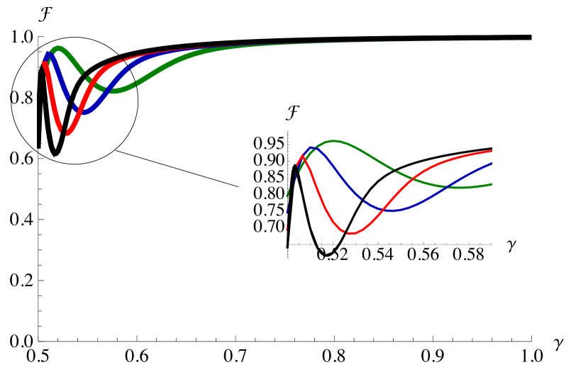
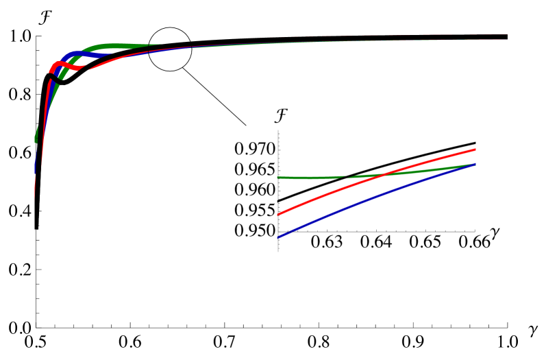
Figure 11: Fidelity between the symmetry-adapted and exact quantum states, as a function of the interaction strength $\gamma$, shown for the ground state (even parity, left) and the first excited state (odd parity, right). In both cases, the plots show that for increasing $N=10,\,20,\,40$ and $50$ the fidelity rises more sharply to $1$ as we move away from the phase transition (at $\gamma_{c}=0.5$). In all cases $\omega_{A}=1$. (Color online.)

VII Discussion and Conclusions

By means of the symmetry properties of the Dicke Hamiltonian, we found analytic expressions for the ground and first excited states, which allows also to determine in closed form the expectation values of matter and field observables. The procedure was the following: we calculated the expectation value of the Hamiltonian with respect to the tensorial product of Weyl and SU(2) coherent states. This expectation value defines a function called energy surface depending on phase space variables and parameters. We then determine the degenerate and minimum critical points of the energy surface. The minimum critical points yield the expressions (10) which give the mimimum energy of the system together with information about the quantum phase transition present in the Dicke Hamiltonian. This quantum phase transition occurs when $\tilde{\omega}_{A}\,\tilde{\omega}_{F}=4\tilde{\gamma}^{2}$. Afterwards we restore the symmetry exhibited for the Dicke Hamiltonian by means of the projection of the states to definite parity of the excitation number operator. These symmetry considerations lead to determine the ground and first excited states together with important differences from the mean field results for some fluctuations of the matter and field observables. Additionally they provide us with the joint probability distribution functions of the number of photons and excited atoms.

The condition to transit from the normal to the superradiant regimes is very difficult to satisfy for optical systems because the available dipole coupling strengths are usually smaller than the transition frequency. Some proposals to overcome these problems have been discussed in nagy , where it is stated that the quantum motion of a Bose-Einstein condensate trapped in an optical cavity can be used to realize the Dicke model. Indeed, this has been reported in baumann , where the Dicke Hamiltonian has been physically realized in a superfluid gas moving in an optical cavity. However, the feasibility of reaching the superradiant phase of the field-matter interaction is still under debate nataf ; viehman .

The predicted $\sqrt{N}$–behaviour for the collective $N$–atom interaction strength of the model has been observed experimentally in circuit QED for up to $5$ qubits fink .

In this work we have shown that semi-classical states adapted to the symmetry of the Hamiltonian are an excellent approximation to the exact quantum solution of the ground and first excited states of the Dicke model in the superradiant phase. Their overlap to the exact quantum states is very close to $1$ except in a close vicinity of the quantum phase transition (cf. Fig.(11)), whereas that of the ordinary coherent states would be at best equal to $1/2$ (cf. Eq.(18)). Our projected states have analytical forms in terms of the model parameters and allow us to calculate analytically the expectation values of field and matter observables. We have found that in the superradiant regime the fluctuation $(\Delta\hat{q})^{2}$ of the first quadrature of the electromagnetic field is different from the results obtained via the standard coherent states and its value grows as a linear function of $N$. Something similar happens for the fluctuation in the dipole transition operator $(\Delta\hat{J}_{x})^{2}$, where one finds a quadratic dependence in the number of atoms. Both these results contradict those obtained previously emary . The expectation values of the number of photons and of the number of excited atoms were also studied, finding that there are no singularities at the phase transition. Those found previously nagy are an artifact of an inappropriate truncation of the Hamiltonian. The joint probability distribution functions for the ground and first excited states were shown, which may be used to characterize the states of atoms in a cavity according to whether $n_{e}+\nu$ has an even or odd value.

In a future contribution, we will evaluate other properties like the entanglement entropy between field and matter, and the squeezing parameter for the electromagnetic field and atomic components, which has been the subject of much interest citevidal.

Finally we want to remark that the present formalism allows for a simplification of the exact quantum calculation by considering an expansion of Dicke and photon number states running from a minimum value $\lambda_{min}$ to $\lambda_{max}$, where these values can be estimated from $\lambda_{c}$ and its corresponding fluctuations $\delta\lambda_{c}$ as functions of $\gamma$, the coupling parameter between the field and matter. The same simplification can immediately be done in the proposed state (13) without changing the obtained results for all the expectation values and probability distributions.

VIII Acknowledgments

This work was partially supported by CONACyT-México (project-101541), FONCICYT (project-94142), and DGAPA-UNAM.

References

- (1) R. H. Dicke, Phys. Rev. 93, 99 (1954).
- (2) E. A. Power and S. Zineau, Philos. Trans. R. Soc. A 251, 427 (1959).
- (3) E. T. Jaynes and F. W. Cummings, Proc. IEEE 51, 89 (1963).
- (4) M. Tavis and F. W. Cummings, Phys Rev. 170, 379 (1968).
- (5) K. Hepp and E. H. Lieb, Phys. Rev. A 8, 2517 (1973).
- (6) K. Rzazewski, K. Wodkiewicz, and M. Zacowicz, Phys. Rev. Lett. 35 (1975) 432; K. Rzazewski and K. Wodkiewicz, Phys. Rev. A 13, 13 (1976).
- (7) I. Bialynicki-Birula and K. Rzazewski, Phys. Rev. A 19, 301 (1979).
- (8) S. Sivasubramanian, A. Widom, and Y. N. Sivrastava, Physica A 301, 241 (2001).
- (9) O. Castaños, E. Nahmad-Achar, R. López-Peña, and J.G. Hirsch in Symmetries in Nature AIP Conference Proceedings 1323, p. 40-59 Eds. L. Benet, P.O. Hess, J.M. Torres, K.B. Wolf (Melville, New York, 2010).
- (10) F. Dimer, B. Estienne, A.S. Parkins, and H.J. Carmichael, Phys. Rev. A 75, 013804 (2007).
- (11) D. Nagy, G. Konya, G. Szirmani, and P. Domokos, Phys. Rev. Lett. 1047, 130401 (2010).
- (12) K. Bauman, C. Guerlin, F. Brennecke, and T. Esslinger, Nature 464, 1301 (2010).
- (13) O. Castaños, E. Nahmad-Achar, R. López-Peña, and J.G. Hirsch, Phys. Rev. A (in press).
- (14) C. Emary and T. Brandes, Phys. Rev. E 67, 066203 (2003); C. Emary and T. Brandes, Phys. Rev. Lett. 90, 044101 (2003); N. Lambert, C. Emary and T. Brandes, Phys. Rev. Lett. 92, 073602 (2004).
- (15) T. Holstein and H. Primakoff, Phys. Rev. 58, 1098 - 1113 (1940).
- (16) O. Castaños, R. López-Peña, E. Nahmad-Achar, J.G. Hirsch, E. López-Moreno, and J. E. Vitela, Phys. Scr. 79, 065405 (2009).
- (17) O. Castaños, E. Nahmad-Achar, R. López-Peña, and J.G. Hirsch, Phys. Scr. 80, 055401 (2009).
- (18) K.T. Hecht, The Vector Coherent State Method and Its Applications to Problems of Higher Symmetries (Springer, Berlin 1987).
- (19) F.T. Arecchi, E. Courtens, R. Gilmore, and H. Thomas, Phys. Rev. A6, 2211 (1972).
- (20) R. Gilmore, Catastrophe Theory for scientists and engineers, (Wiley, New York, 1981).
- (21) O. Castaños, E. Nahmad-Achar, R. López-Peña, and J.G. Hirsch, work in progress.
- (22) W.K. Wooters, Phys. Rev. D 23, 357 (1981).
- (23) P. Nataf and C. Ciuti, Nature Comm. 1:72 (2010).
- (24) O. Viehmann, J. von Delft, F. Marquardt, arXiv:1103.4639.
- (25) J. M. Fink et al., Phys. Rev. Letters 103, 083601 (2009).
- (26) J. Vidal, S.Dusuel, T. Barthel, J. Stat. Mech, P01015 (2007).