Investigations of three, four, and five-particle exit channels of levels in light nuclei created using a ⁹C beam

Abstract

The interactions of a $E/A$=70-MeV ⁹C beam with a Be target was used to populate levels in Be, B, and C isotopes which undergo decay into many-particle exit channels. The decay products were detected in the HiRA array and the level energies were identified from their invariant mass. Correlations between the decay products were examined to deduce the nature of the decays, specifically to what extent all the fragments were created in one prompt step or whether the disintegration proceeded in a sequential fashion through long-lived intermediate states. In the latter case, information on the spin of the level was also obtained. Of particular interest is the 5-body decay of the ⁸C ground state which was found to disintegrate in two steps of two-proton decay passing through the ⁶Be_g.s. intermediate state. The isobaric analog of ⁸C_g.s. in ⁸B was also found to undergo two-proton decay to the isobaric analog of ⁶Be_g.s. in ⁶Li. A 9.69-MeV state in ¹⁰C was found to undergo prompt 4-body decay to the 2p+2$\alpha$ exit channel. The two protons were found to have a strong enhancement in the diproton region and the relative energies of all four p-$\alpha$ pairs were consistent with the ⁵Li_g.s. resonance.

I INTRODUCTION

The ground and excited states of many light proton-rich nuclei decay by the emission of protons and other charged particles. A number of these states disintegrate into just protons and alpha particles and other very light fragments. Well known examples are the ground states of ⁶Be and ⁹B which decay to the 2p+$\alpha$ and the p+2$\alpha$ exit channels. Such states can be studied with resonance decay spectroscopy where all of the decay fragments are detected. The excitation energy of the parent state can be determined from the invariant mass of the detected decay products. For exit channels with more than two fragments, the angular and energy correlations between the fragments can provide information on the spin of the state and the nature of its decay, i.e., whether the decay proceeds through a series of sequential 2-body decay steps or via a more prompt process.

In this work we have utilized a ⁹C beam to study a number of such states which were formed via nucleon knockout and more complicated reactions. Of particular interest is the ground state of ⁸C which is known to be unstable to the 5-body exit channel 4p+$\alpha$. Information about ⁸C is rather sparse and the 5-body exit channel has never been observed experimentally. A particular question for ⁸C disintegration and other many-particle exit channels detected in this work is whether the final particles were created in one fast process or in a series of sequential steps with the creation of long-lived intermediate states? Of course there is not always a clear demarcation between such processes. If the lifetime of the intermediate states becomes too short, does it make sense to still describe the decay as two or more sequential steps?

One situation that is particularly clear is the two-proton decay described by Goldansky Goldansky60 where no intermediate state can be energetically accessed. Examples of this are the two-proton decays of ⁴⁵Fe Miernik07 and ⁵⁴ZnBlank05 . In cases where this condition is not reached, Bochkarev et al. considered a distinction in the decay type based on the width of the potential intermediate state. For a 3-body exit channel, if the potential intermediate state has a width $\Gamma_{I}$ which is of the same magnitude as the kinetic energy $E_{k}^{1}$ released in the decay to this state, then its decay was deemed democratic, i.e., all energy scales in the subsystems and the three-body systems are comparable. We have constructed the ratio

$$R_{E}=\frac{\Gamma_{I}}{E_{k}^{1}}$$ (1)

to quantify this. Thus if $R_{E}\ll$ 1, the decay is sequential, where as if $R_{E}\geq$ 1, then the decay is democratic. Large values of $\Gamma_{I}$ and thus of $R_{E}$ imply a short-lived intermediate state and thus a difficulty in distinguishing the two decay steps. Another way to quantify this is to estimate the separation $d_{E}$ of the fragments from the first step at average time of the second decay step, i.e., the decay of the the intermediate state. This separation is

$$d_{E}=\sqrt{\frac{2E_{k}^{1}}{\mu}}\frac{\hbar}{\Gamma_{I}},$$ (2)

where $\mu$ is the reduced mass of products produced in the first decay step. If $d_{E}$ is much larger than the typical nuclear diameter ($\sim$5 fm), then the two decay steps are well separated and cannot influence each other through nuclear processes.

Again we emphasize that the quantities $R_{E}$ and $d_{E}$ do not provide sharp distinctions between prompt and sequential processes. For intermediate values of these quantities, one may consider a decay process that is basically sequential, but where final-state interactions between the products from the different decay steps are still important. If these final-state interactions do not washout sequential signals such as the invariant mass of the intermediate state deduced from its decay products, or the angular correlations between the sequential decay steps, then one might still claim that the decay has a strong sequential character. However detailed predictions for the correlations may require a many-body calculation.

The angular correlations in sequential decay are a consequence that the system passes through an intermediate state of well defined spin. Not all potential sequential decay scenarios have such correlations, for example if the intermediate state is $J$=0, or the orbital angular momentum removed in either step is zero. Thus the search for these correlations cannot be performed for all cases.

An example of a truly sequential process is the decay of the ground state of ⁹B to the p+2$\alpha$ exit channel. The decay begins by a proton emission to the ground state of ⁸Be which has a very small width ($\Gamma_{I}$=6.8 eV). Here, $R_{E}$=3.6$\times$10^-5 and $d_{E}$=6.1$\times$10⁵ fm which indicates that there are no significant interactions between the proton from the first step and the $\alpha$ particles from the second step.

The nucleus ⁶Be_g.s. which decays to the 2p+$\alpha$ channel provides an example of democratic decay. The possible intermediate state ⁵Li_g.s. is very wide ($\Gamma_{E}$=1.23 MeV), but most of the strength associated with this state is energetically inaccessible in ⁶Be_g.s. decay (see Fig. 3). Sequential decay is only possible through the low-energy tail of this resonance. Thus ⁶Be_g.s. is thus almost a Goldansky-type decay. In a sequential scenario, the mean energy released in the first step can be determined in an R-matrix approximation (Sec. III) as $E_{k}^{1}$=0.64 MeV and this gives $R_{E}$=1.92 and $d_{E}$=6.5 fm, which is not in the realm of a truly sequential decay. Experimental studies show no evidence of the angular correlations expected in a sequential scenario Geesaman77 (see also Sec. IV.1) and a good description of the decay correlations, the decay energy and its width can be obtained with a 3-body cluster model Grigorenko09 .

In this work we report on an experimental investigation of particle-unstable states in Be, B, and C isotopes all of which undergo disintegration into 3 or more final fragments. In each case, we have measured correlations between these fragments to deduce the nature of the decay and to determine to what extent sequential and prompt many-body processes are involved. The states reported on were all created as projectile-like fragments after the interaction of a secondary $E/A$=70 MeV ⁹C beam with a Be target. One case of particular interest is the 4p+$\alpha$ decay of ⁸C_g.s. As ⁶Be_g.s. is a possible intermediate state in the decay of this level, we have obtained improved data for the ⁶Be system using a $E/A$=70 MeV ⁷Be secondary beam to help in the interpretation of the ⁸C data. Some of the ⁸C results have already been published in Ref. Charity10 . The details of the experiment are discussed in Sec. II. Results for each of the examined states are given in Sec. IV and the conclusions of this work are presented in Sec. V.

II EXPERIMENTAL METHOD

A primary beam of $E/A$=150-MeV ¹⁶O was extracted from the Coupled Cyclotron Facility at the National Superconducting Cyclotron Laboratory at Michigan State University with an intensity of 125 pnA. This beam bombarded a ⁹Be target producing $E/A$=70.0-MeV ⁹C and ⁷Be projectile-fragmentation products which were selected by the A1900 separator with a momentum acceptance of $\pm$0.5%. The ⁹C secondary beam had an intensity of 1.6$\times$10⁵ s^-1 with a purity of $\sim$65% with the main contaminant being ⁶Li. The ⁷Be beam had an intensity of 4$\times$10⁷ s^-1 with a purity of $\sim$90%.

The two secondary beams impinged on a 1-mm-thick target of ⁹Be. Charged particles produced in the reactions with this target were detected in the HiRA array Wallace07 . For this experiment, the array consisted of 14 $E$-$\Delta E$ [Si-CsI(Tl)] telescopes located at a distance 90 cm downstream from the target. The angular coverage of the array is illustrated in Fig. 1 and it subtended polar angles from 1.4^∘ to 13^∘. Each telescope consisted of a 1.5-mm thick, double-sided Si strip $\Delta E$ detector followed by a 4-cm thick, CsI(Tl) $E$ detector. The $\Delta E$ detectors are 6.4 cm$\times$6.4 cm in area with each of the faces divided into 32 strips. Each $E$ detector consisted of four separate CsI(Tl) elements each spanning a quadrant of the preceding Si detector. Signals produced in the 896 Si strips were processed with the HINP16C chip electronics Engel07 . For the ⁹C beam, the time of flight measured between a thin scintillator foil in the A1900 extended focal plane and the HiRA trigger was used in conjunction with the energy loss in this foil to reject most of the beam contaminants.

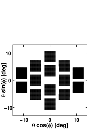
Figure 1: The angular coverage of the HiRA array used in this experiment.

The energy calibration of the Si detectors was obtained with a ²²⁸Th $\alpha$-particle source. The particle-dependent energy calibrations of the CsI detectors were achieved with cocktail beams selected with the A1900 separator. These include protons ($E/A$=60 and 80 MeV), $\alpha$-particles ($E/A$=60 and 80 MeV), deuterons ($E/A$=21 and 59 MeV), tritons ($E/A$=27 and 36 MeV), ³He ($E/A$=37 and 103 MeV) and ⁶Li ($E/A$=60 and 80 MeV) beams.

The HiRA telescopes have excellent isotope separation for the all of the light fragments of interest in this work and multiple fragments within a single telescope can be identified Charity07 . The gains for the Si amplifiers were setup for the detection of hydrogen and helium isotopes. Some information on lithium isotopes is used in this work, but lower-energy Li fragments saturated the Si shaping amplifiers and could not be identified (see later).

III Simulations

The effect of the detector acceptance and resolution is quite important when extracting decay widths, branching ratios and correlations between the fragments. These effects have been extensively studied using Monte Carlo simulations that include the angular acceptance and the angular and energy resolutions of the detectors, the energy loss Ziegler85 and small-angle scattering Anne88 of the fragments as they leave the target, and the beam-spot size. These simulations have proven quite reliable in past experiments with HiRA Charity07 ; Charity08 .

A number of different types of simulations are described in this work including both sequential and prompt decay processes. However, the predicted resolution of the excitation energy of a level was found to be mostly insensitive to the details of the decay process, but is largely determined from the detector properties.

In simulating sequential 3-body decays, where the width of the intermediate state is significant, we have used the R-matrix formalism Lane58 ; Barker99 to predict the distribution of $E_{T}$, the total kinetic energy released, and $E_{x}$=$E_{T}$-$E_{k}^{1}$, the kinetic energy released in the second step;

$$N(E_{T},E_{x})\sim\frac{\Gamma_{1}(E_{T},E_{x})}{[E_{T}-Q_{1}-\Delta_{tot}(E_{T})]^{2}+(1/4)\Gamma_{tot}^{2}(E_{T})}$$ (3)

where

$$\Gamma_{tot}(E_{T})=\int_{0}^{E_{T}}\Gamma_{1}(E_{T},E_{x})dE_{x},$$ (4)

$$\Delta_{tot}(E_{T})=\int_{0}^{\infty}\Delta_{1}(E_{T},E_{x})dE_{x},$$ (5)

$$\Gamma_{1}(E_{T},E_{x})=2\gamma_{1}^{2}P_{1\ell}(E_{T}-E_{x})\rho(E_{x}),$$ (6)

$$\Delta_{1}(E_{T},E_{x})=-\gamma_{1}^{2}[S_{1\ell}(E_{T}-E_{x})-S_{1\ell}(Q_{1}-E_{x})]\rho(E_{x}),$$ (7)

$$\rho(E_{x})=c\frac{\Gamma_{2}(E_{x})}{[E_{x}-Q_{2}-\Delta_{2}(E_{x})]^{2}+(1/4)\Gamma_{2}^{2}(E_{x})},$$ (8)

$$\int_{0}^{\infty}\rho(E_{x})dE_{x}=1,$$ (9)

$$\Gamma_{2}(E_{x})=2\gamma_{2}^{2}P_{2\ell}(E_{x}),$$ (10)

$$\Delta_{2}(E_{x})=-\gamma_{2}^{2}[S_{2\ell}(E_{x})-S_{2\ell}(Q_{2})],$$ (11)

$$P_{\ell}(E)=\frac{ka}{F_{\ell}(ka)^{2}+G_{\ell}(ka)^{2}},$$ (12)

$$S_{\ell}(E)=\frac{F^{\prime}_{\ell}(ka)F_{\ell}(ka)+G^{\prime}_{\ell}(ka)G_{\ell}(ka)}{F_{\ell}(ka)^{2}+G_{\ell}(ka)^{2}},$$ (13)

$$a=1.45\rm{fm}(A_{1}^{1/3}+A_{2}^{1/3}),$$ (14)

$F$ and $G$ are regular and irregulat Coulomb wavefunctions, $k$ is the wave number, $c$ is a normalization constant determined from Eq. (9), $\gamma_{1}^{2}$ and $\gamma_{2}^{2}$ are the reduced widths associated with the first and second decay steps, and $Q_{1}$ and $Q_{2}$ are the centroids associated with $E_{T}$ and $E_{x}$, respectively. Angular correlations in sequential decay are calculated from Refs. Biedenharn53 ; Frauenfelder53 .

The reduced width can be expressed as

$$\gamma^{2}=S\theta^{2}_{sp}\frac{\hbar^{2}}{\mu a^{2}}$$ (15)

where $S$ is the spectroscopic factor and $\theta^{2}_{sp}$, the single-particle dimensionless reduced width, is

$$\theta^{2}_{sp}=\frac{a}{2}\frac{u^{2}(a)}{\int_{0}^{a}u^{2}(r)dr}.$$ (16)

Here $u(r)/r$ is the single-particle radial wave function calculated with a Coulomb plus Wood-Saxon potential with standard parameters for radii and diffuseness ($r_{0}$=1.25 fm, $r_{C}$=1.3 fm, and $a$=0.65 fm) and the depth adjusted to fit the resonance energy.

IV RESULTS

The deduced properties of the levels investigated in this study are summarized in Table 1 including their centroids, widths, and decay modes. More detailed discussion for each case are contained in the rest of this section including comparison with the evaluated quantities from the ENSDF database ENSDF . Excitation energies are determined from the invariant mass method, i.e., the total kinetic energy of the fragments in their center-of-mass reference frame minus the decay Q value.

Table 1: The excitation energy, width, spin and isospin of states for which new information is determined.

nucleus	decay	branching	exit	$E^{*}$	$\Gamma$	$J^{\pi}$	$T$
		ratio	channel	[MeV]	[keV]
7B	p+6Beg.s.	81$\pm$10%	3p+$\alpha$	0.0	801$\pm$20		3/2
8B	p+7Be4.57		p+3He+$\alpha$	5.93$\pm$0.02	850$\pm$260	3, 4	1
8B	p+7Be6.73		p+3He+$\alpha$	8.15$\pm$0.20	950$\pm$320		1
8B	2p+6LiIAS	$\sim$97.5%	2p+6Li	10.619$\pm$0.009	$<$60	0+	2
	2p+6Li2.18	$\sim$1.0%	2p+d+$\alpha$
	2p+d+$\alpha$	$\sim$1.5%
8Be	p+7Li4.63		p+t+$\alpha$	22.96$\pm$.02	680$\pm$146	3, 4	1
8C	2p+6Beg.s.	100%	4p+$\alpha$	0.0	130$\pm$50	0+	2
9B	$\alpha$+5Li	97.2$\pm$0.5%	p+2$\alpha$	11.70$\pm$0.02	880$\pm$80	3/2-,5/2+,7/2-	1/2
	p+8Be3.03	2.8$\pm$0.5%	p+2$\alpha$
9B	p+8BeT=0+1		p+2$\alpha$	16.99$\pm$0.03	22$\pm$5	1/2-	3/2
9B	p+8Be19.069		2p+7Li	20.64$\pm$0.10	450$\pm$250
10C	p+9B2.345		2p+2$\alpha$	8.54$\pm$0.02	$<$200
10C	2p+2$\alpha$	48%	2p+2$\alpha$	9.69	490		1
	$\alpha$+6Be	35%	2p+2$\alpha$
	p+9B2.34	17%	2p+2$\alpha$
10C			2p+2$\alpha$	10.48$\pm$0.2	$<$200
10C			2p+2$\alpha$	11.44$\pm$0.2	$<$200

IV.1 ⁸C ground state

The ground state of ⁸C is unstable to disintegration into four protons and an $\alpha$ particle. The distribution of ⁸C excitation energy reconstructed from the 4p+$\alpha$ channel following neutron knockout of ⁹C beam particles is displayed in Fig. 2(a). The excitation energy was determined assuming the ⁸C mass excess of 35.094 MeV obtained from the 2003 mass evaluation of Ref. Audi03 . The mass excess is needed to calculate the decay Q value. The excitation-energy spectrum shows a strong peak located near zero excitation energy indicating that we have populated the ground state of ⁸C. The long-dashed curve shows the simulated shape, including detector response, based on the evaluated mass excess and the listed ⁸C decay width of 230 keV. This curve also contains a background contribution which is indicated by short-dashed curve. The simulated shape is both wider and shifted up in energy compared to the experimental peak suggesting that the evaluated mass excess and width used in the simulations are incorrect.

In order gain a better understanding of the magnitude of the experimental uncertainties associated with this measurement, we have investigated the line shape of the ⁶Be ground state formed in neutron knockout reactions from the ⁷Be beam. In the ⁹C and ⁷Be neutron knockout reactions, the beam velocities, target thickness, and detector apparatus were identical and thus systematic errors are expected to be the same. The reconstructed ⁶Be excitation-energy spectrum from the detected 2p+$\alpha$ events is displayed in Fig. 2(b). This spectrum contains a peak at zero energy associated with the ground state and a wider peak at $\sim$1.7 MeV associated with the first excited state. For the ground-state peak, the solid curve in this figure shows the simulated spectrum, again including a background contribution (including a contribution from the first excited state) which is indicated by the short-dashed curve. The tabulated ⁶Be mass excess and decay width were used in this simulation which reproduces the experimental result very well, strongly suggesting that the disagreement of the simulation with the data for ⁸C is not an experimental artifact. The experimental FWHM of the ⁶Be ground-state peak is 214$\pm$10 keV, significantly greater than its intrinsic width of $\Gamma$=92$\pm$6 keV. Thus the agreement between the ⁶Be_g.s. data and simulation indicates that we can correctly account for the experimental resolution.

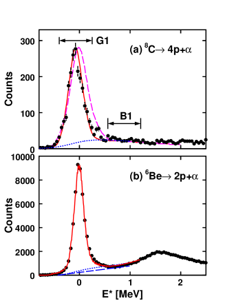
Figure 2: (Color online) Excitation-energy spectra for (a) ⁸C fragments produce in neutron knockout from the ⁹C beam and (b) ⁶Be fragments produced in neutron knockout from the ⁷Be beam. In both cases, the curves show simulated ground-state distributions (see text). The solid curve in (a) is a fit to the data with a background indicated by the dotted curve. The dashed curve is the simulated response based on the tabulated peak location and width. In dotted and dashed curves in (b) are the two possible background distribution considered in the text.

The solid curve in Fig. 2(a) shows the results of a simulation where both the ⁸C mass excess and its decay width were adjusted to best reproduce the experimental peak. The fitted mass excess is 35.030$\pm$0.030 MeV and the fitted width is 130$\pm$50 keV.

Previous measurements of the mass excess and decay width were made in Refs. Robertson74 ; Robertson76 ; Tribble76 using transfer reactions. Of these, only the 1976 work of Tribble et al. Tribble76 has more than a handful of ⁸C events. The reaction studied was ¹²C(⁴He,⁸He)⁸C and the ⁸He fragments were detected. The extracted mass excess was 35.10$\pm$0.03 and the decay width was 230$\pm$50 keV and 183$\pm$56 keV assuming Breit-Wigner and Gaussian intrinsic lines shapes, respectively. As in the present work, the experimental resolution was significant.

The ⁸C ground state is quite unusual in having a five-particle exit channel. It is of interest to determine whether this state disintegrates directly into five pieces or proceeds in a sequential process of two or more steps through intermediate states. Figure 3 shows the levels of possible interest in the decay. Of the possible intermediate states, the ⁶Be ground state is the narrowest (longest lived) and easiest to detect experimentally. In each detected 4p+$\alpha$ event, one can find 6 ways to reconstruct a ⁶Be decay as a 2p+$\alpha$ subset. For each of these ways, a ⁶Be excitation energy is determined. We use gate $G1$ in Fig. 2(a) to select out the ground-state events. The resulting excitation-energy spectrum of all these potential ⁶Be candidates is displayed in Fig. 4(a) as data points. As there can be at most only one ⁶Be ground-state fragment per event, at least 5/6 th of the spectrum corresponds to incorrectly reconstructed ⁶Be fragments and these form a background. The experimental spectrum clearly displays a peak centered near zero energy associated with the ⁶Be ground state on a background of approximately Gaussian shape.

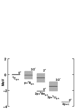
Figure 3: Levels of interest in the decay of the ⁸C and ⁷B ground states.

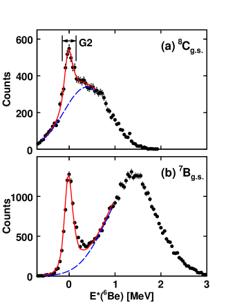
Figure 4: (Color online) The spectrum of all possible reconstructed ⁶Be excitation energies for events in the ground states of (a) ⁸C and (b) ⁷B. The data points are the experimental data, while the solid curves show fits to the ⁶Be ground-state region with the dashed curves showing the fitted background.

To determine what fraction of the ⁸C events decay through ⁶Be_g.s., we have fitted the spectrum in Fig. 4(a) with two components; a ⁶Be_g.s. component with shape taken from the experimental peak in Fig. 2(b) obtained with the ⁷Be beam and a background component taken to be Gaussian in the immediate vicinity of the ⁶B_g.s. peak. In order to use the experimental ⁶Be_g.s. line shape from Fig. 2(b), one has to first subtract the small background under this peak. The short and long-dashed curves in this figure show two possible backgrounds which were considered. The short-dashed curve is associated with the solid curve obtained using a symmetric Breit-Wigner line shape. The use of the long-dashed background curve would imply a slightly asymmetric ⁶Be_g.s. line shape which has an enhanced higher-energy tail. A small degree of asymmetry is not unreasonable.

The resulting fit (using the original ⁶Be background) is shown by the solid curve in Fig. 4(a) where the Gaussian background is indicated by the dashed curve. Taking into account both possible ⁶Be backgrounds, these fits imply that, on average, 1.01$\pm$0.05 ⁶Be_g.s. fragments are created in each ⁸C_g.s. decay, i.e. essentially all decays pass through ⁶Be_g.s..This number was corrected for the small background under the ⁸C_g.s. peak itself [dotted curve in Fig. 2(a)], using the the region $B1$ to estimate the ⁶Be probability associated with this background.

In many ways, the decay of ⁸C_g.s to 2p+⁶Be_g.s. is similar to the decay of ⁶Be_g.s. to 2p+$\alpha$. In each case, both the initial and final states are $J^{\pi}$=0⁺ and the possible intermediate states (⁷B_g.s. and ⁵Li_g.s) are $J^{\pi}$=3/2^-. These intermediates states are both wide, but only their low-energy tails are energetically accessible. Both decays are democratic; $R_{E}$=1.2 and 1.9 and $d_{E}$=8.8 and 6.5 fm for ⁸C and ⁶Be, respectively. Thus the disintegration of ⁸C_g.s. is novel having two sequential steps of democratic two-proton decay. To investigate this possibility, it is useful to separate out experimentally the protons from the first and second decay steps. However, it is not possible to do this with 100% certainty for all decays.

For a fraction of the events it is possible to make this separation with reasonable precision. To this end, we have selected events where one, and only one, of the 6 possible reconstructed ⁶Be fragments has an excitation energy associated with the ground-state peak indicated by the region $G2$ in Fig. 4(a). For the events which survive this criteria, the identities of the ⁶Be_g.s. decay products are obvious.

Some events from the tails of the ⁶Be_g.s. peak lie outside the $G2$ region and will be rejected. Also, and more importantly one can have the situation that the correct ⁶Be fragment is in the high or low-energy tail outside of the gate and an incorrectly identified ⁶Be fragment lies within the $G2$ gate. Such an event will not be rejected, but the identities of the protons from the first and second steps will be incorrect. Monte Carlo simulations were used to optimize the width of the $G2$ region so as to obtain the best compromise between event-rejection and mis-identification.

With the chosen gate width we select only 30% of the ⁸C_g.s. events and, of these, we estimate that a selected event is incorrectly identified 30% of the time. While this is significant, these misidentifications involve cases were the two protons assigned to one of the decay steps are actually from the two separate steps. As the two steps are separated by a ⁶Be_g.s. fragment with $J^{\pi}$=0⁺, there is no angular correlations between the protons from the two steps and these misidentified events will give rise only to smooth backgrounds in the correlation plots.

The energy and angular correlations between the particles produced in two-proton decay can be described by the hyperspherical Jacobi vectors $\mathbf{X}$ and $\mathbf{Y}$ and their conjugate momenta $\mathbf{k}_{x}$ and $\mathbf{k}_{y}$. There are two independent ways of defining the coordinates which are referred to as the “T” and “Y” systems. These are illustrated in Fig. 5 where the core (fragment 3 in the “T” system or fragment 2 in the “Y” system) is the ⁶Be_g.s. fragment in the first 2p decay and the $\alpha$ particle in the second 2p decay. In terms of the position vectors $\mathbf{r}_{i}$, momentum vectors $\mathbf{k}_{i}$ and masses $m_{i}$ ($i$=1, 2, and 3) the Jacobi coordinates are

$$\mathbf{X} = \mathbf{r}_{1}-\mathbf{r}_{2}\,,$$ (17a)

$$\mathbf{Y} = \frac{m_{1}\mathbf{r}_{1}+m_{2}\mathbf{r}_{2}}{m_{1}+m_{2}}-\mathbf{r}_{3}\,,$$ (17b)

$$\mathbf{k}_{x} = \frac{m_{2}\mathbf{k}_{1}-m_{1}\mathbf{k}_{2}}{m_{1}+m_{2}}\,,$$ (17c)

$$\mathbf{k}_{y} = \frac{m_{3}(\mathbf{k}_{1}+\mathbf{k}_{2})-(m_{1}+m_{2})\mathbf{k}_{3}}{m_{1}+m_{2}+m_{3}}.$$ (17d)

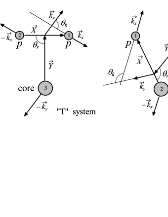
Figure 5: Independent “T” and “Y” Jacobi systems for the core+$N$+$N$ three-body system in coordinate and momentum spaces.

Of the six degrees of freedom required to define the $\mathbf{k}_{x}$ and $\mathbf{k}_{y}$ distributions, three describe the Euler rotation of the decay plane and one is constrained from energy conservation. Thus the complete correlation information can be described by two variables which we take as $E_{x}/E_{T}$ and $\theta_{k}$, where $E_{x}$ is the energy associated with the $X$ coordinate,

$$E_{x}=\frac{(m_{1}+m_{2})k_{x}^{2}}{2m_{1}m_{2}},$$ (18)

$E_{T}$ is the total three-body energy and $\theta_{k}$ is the angle between the Jacobi momenta,

$$\theta_{k}=\frac{\mathbf{k}_{x}\cdot\mathbf{k}_{y}}{k_{x}k_{y}}.$$ (19)

For each event, there are two ways of labeling the two protons and thus there are two possible values of the [$E_{x}/E_{T}$,$\cos(\theta_{k})$] coordinate, both of which are used to increment the correlation histograms. For the “T” system, this produces a symmetrization of the angular distributions about $\cos(\theta_{k})$=0.

Distributions constructed in the two Jacobi systems are just different representations of the same physical picture. Each Jacobi system can reveal different aspects of the correlations. The Jacobi “Y” system is particularly useful if the two protons are emitted sequentially through an intermediate state. In this case, $E_{x}$ is the kinetic energy released in the second step and $\theta_{k}$ is the angle between the two decay axes. The Jacobi “T” system can have a similar interpretation for a diproton decay with an intermediate ²He state.

The projected correlations in both the “T” and “Y” systems are plotted in Fig. 6 for the second decay step of ⁸C_g.s., i.e., the 2p decay of the ⁶Be_g.s. intermediate state. These can be compared to results from the ⁷Be beam in Fig. 7, where ⁶Be_g.s. is formed more directly following a neutron-knockout reaction. In this case, the statistical uncertainties are significantly smaller and there are no misidentified events. A consistency between the projected correlations in Fig. 6 and 7 is necessary if the ⁸C_g.s. level disintegrates through ⁶Be_g.s. and indeed the corresponding projected correlations are quite similar in the two figures.

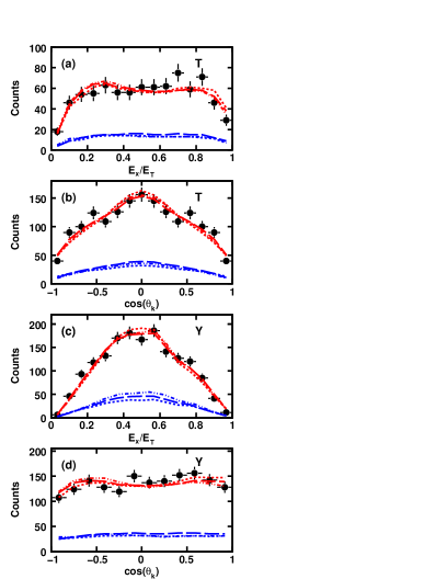
Figure 6: (Color online) Projected correlations in (a,b) “T” and (c,d) “Y” Jacobi systems for the three-body decay of ⁶Be formed in the second step of ⁸C_g.s. decay. Angular correlations are shown in (b) and (d) and energy correlations are shown in (a) and (c). The data points are the experimental data, while simulated results are indicated by the curves which pass through the data points. The lower curves are estimates of the “backgrounds” of incorrectly identified events. The short and long-dashed and solid curves are associated with simulations (A), (B) , and (C), respectively (see text).

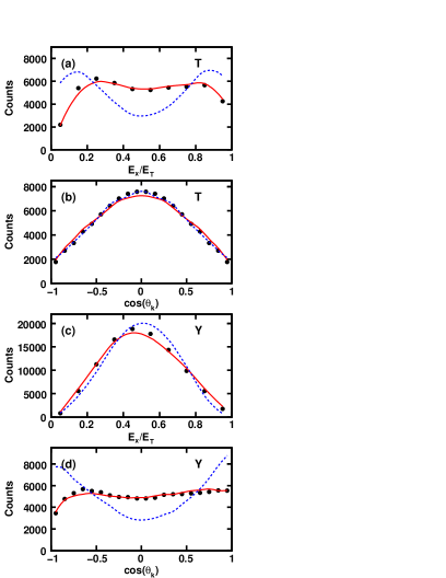
Figure 7: As for Fig. 6, but now for ⁶Be_g.s. events produced via neutron knockout from the ⁷Be beam. The solid and dashed curves show predictions of the 3-body cluster model and a sequential-decay calculation, respectively.

In order to make more detailed comparisons of the experimental ⁶Be correlations in Figs. 6 and 7, we have made extensive Monte-Carlo simulations including the effect of the detector response and the event selection requirements. The results from the ⁷Be beam in Fig. 7 are compared to simulations where the effect of the detector resolution and acceptance is considered with no misidentification or selection bias. The detector effects induce only small modifications to the projected correlations in this case. The solid curves are predicted distributions from the Quantum-Mechanical 3-body cluster model of Ref. Grigorenko09 (Calculation P2 in that reference). This model reproduces the experimental total energy $E_{T}$, $\Gamma$, and the experimental correlations in Fig. 7. These predicted correlations will therefore be used in the simulations in the disintegration of ⁸C.

The dashed curves in Fig. 7 are from an R-matrix approximation of sequential 2-proton emission from ⁶Be_g.s. through the ⁵Li_g.s. intermediate state as described in Sec. III. The angular correlations in this simulation are particularly strong and favor decays where the two sequential decay axes are collinear, i.e. $\cos(\theta_{k})=\pm$1 in the Jacobi “Y” system [see Fig. 7(d)]. This angular correlation is also responsible for the predicted broad minimum in the energy distribution in the Jacobi “T” system [Fig. 7(a)]. However, these features associated with the predicted angular correlation are lacking in the experimental data. This indicates that the decay of ⁶Be_g.s. does not pass through an intermediate state of well defined angular momentum ($J^{\pi}$=3/2^-). Similar conclusions have been made in other studies of ⁶Be_g.s. Geesaman77 ; Bochkarev89 .

Now let us return to ⁶Be_g.s. decay in the process of ⁸C_g.s. disintegration. In order to include the bias from the event selection and the contribution from misidentified events, it is necessary to simulate the first step of ⁸C_g.s. disintegration. For this first decay step, ⁸C$\rightarrow$2p+⁶Be_g.s., we have considered three quite different sets of simulated [$E_{x}/E_{t}$, $\cos(\theta_{k})$] correlations:

1. The momenta of the three fragments are chosen according to available phase-space volume.

2. The [$E_{x}/E_{t}$, $\cos(\theta_{k})$] correlations for the Jacobi “T” system is taken to be the same as for ⁶Be_g.s. decay. Note, as the core mass is different in the ⁸C_g.s. 2-proton decay, the Jacobi-“Y” distribution will not be exactly the same as for ⁶Be_g.s. decay.

3. The decay is treated in the R-matrix approximation as a sequential 2-proton decay through the ⁷B intermediate state in a similar manner as just described for the sequential-2 proton decay of ⁶Be_g.s.. The R-matrix parameters for ⁷B_g.s. are taken from Sec. IV.2.

The short-dashed, long-dashed, and the solid curves in Fig. 6 are the results for ⁶Be_g.s. decay in the second step of ⁸C_g.s. disintegration for simulations (A), (B), and (C), respectively. The curves, which pass through the data points in each panel, include the detector response, the selection bias and the contribution from the incorrectly identified events. The latter contributions are indicated by the lower curves in each panel. In all cases, the three curves from the different simulations almost overlap. Thus the simulated results for ⁶Be_g.s. decay show very little sensitively to the decay correlations in the first ⁸C$\rightarrow$2p+⁶Be_g.s. step. Our assertion that the distributions for the misidentified events show no strong structure is borne out and the simulations for all selected events reproduce the experimental data. Therefore within the statistical errors on the experimental data and uncertainty associated with extracting the data, that correlations in the second step of ⁸C disintegration is consistent with ⁶Be_g.s. decay.

For the first step (2p+⁶Be_g.s.) of ⁸C_g.s. decay, the projected $E_{x}/E_{t}$ and $\cos(\theta_{k})$ distributions for both the Jacobi “T” and “Y” systems are plotted in Fig. 8. The curves in each panel show the simulated distributions and backgrounds from the three simulations discussed above. Again these backgrounds are similar in all the simulations and show relatively smooth behaviors. Clearly, the phase-space simulation (short-dashed curve) is inconsistent with all the experimental projected correlations. Also the simulations using the theoretical ⁶Be correlations (long-dashed curves) does not fit the data in Figs. 8(a) and 8(d) indicating that two-proton correlations are different in the first and second steps.

The sequential decay simulations gives the best description to all the experimental distributions, however, it is clearly not perfect. The predicted angular correlations indicated by the solid curve in Fig. 8(d) show strong enhancements near $\cos(\theta_{k})$=$\pm$1. These angular correlations also cause the large structure predicted for the Jacobi “T” energy distribution of Fig. 8(a). The experimental data also show an enhancement near $\cos(\theta_{k})$=-1, sometimes called the diproton region, however, the corresponding enhancement near $\cos(\theta)$=1 is not evident. In the sequential scenario, $\cos(\theta)$=1 corresponds to the ⁶Be core from the second step being directed towards the proton from the first step. Coulomb final-state interactions may deflect the trajectories and thus suppress the yield near $\cos(\theta)$=1. Alternatively the enhancement near $\cos(\theta_{k})$=-1 may not be related to a sequential angular correlation but rather might be a signature of some “diproton” character of the decay similar to that observed for the 6.57-MeV state in ¹⁰C Charity09 .

The total decay width in the sequential scenario can be estimated as Lane58 ; Barker99

$$\Gamma^{0}=\frac{\Gamma_{tot}(Q_{1})}{1+\gamma_{1}^{2}\int_{0}^{\infty}\frac{dS_{1\ell}(E_{T}-E_{x}}{dEx}\big{)}_{Ex=Q_{1}}\rho(E_{x})dE_{x}}.$$ (20)

The p+⁷B_g.s. spectroscopic factor was calculated with CKI Hamiltonian Cohen65 ; *Cohen67 as $S$=3.20 (8/7) where (8/7) is the center of mass correction. With $\theta^{2}_{sp}$=0.44 from Eq. (16) we estimate $\gamma^{2}_{1}$=4.28 MeV and thus $\Gamma^{0}$=12 keV which is significantly less than the experimental value of 130$\pm$50 keV and thus is clear that this sequential decay scenario cannot provide a total description of the 2-proton decay of ⁸C_g.s..

Given the enhanced “diproton” character of the decay it is useful to consider the diproton decay model which can be treated in the R-matrix formulation of Barker Brown67 together with the diproton cluster decay model developed in Ref. Barker02 ; *Barker03. For the wavefunctions we use the p-shell basis with the CKI Hamiltonian Cohen65 ; *Cohen67.

The diproton decay spectroscopic factor is given as a product of the three terms as in Eq. (7) of Brown67 . For the ⁸C decay these are (8/6)² = 1.78 (the center of mass correction), $G^{2}(p)$=1/2 (the cluster overlap factor) and $C$=1.21 (the p-shell spectroscopic factor for $L$=$S$=0), to give $S_{62}$=1.08. The related single-particle dimensionless reduced width of $\theta^{2}_{sp}$=1.00 is also taken from Barker02 ; *Barker03. The diproton decay width obtained for the experimental decay energy of $Q_{1}$=2.077 MeV is $\Gamma$=88 keV. If we use the older $Q_{1}$ value of 2.147 MeV based on the tabulated masses, the width would be 100 keV. We have assumed a narrow ⁶Be final state. The change coming from a folding with its actual width is small. Our spectroscopic factor $S_{62}$ is a factor of five larger than given by Barker following Eq. (13) of Ref. Barker02 ; *Barker03. We do not know why, but assume that there was an error in Barker’s calculation.

The calculated diproton decay width of $\Gamma$=88 keV is consistent with the experimental value of 130$\pm$50 keV, supporting the interpretation of the enhancement at low $E_{x}$/$E_{T}$ in the Jacobi “T” system [Fig. 8(a)] as a diproton feature. However, the diproton model does not provide a complete description of the experimental correlations. For example in the diproton model, the Jacobi “T” angular distribution is just the distribution of the diproton decay angle, which should be isotropic as the diproton has $J^{\pi}$=0⁺. However the experimental distribution in Fig. 8(b) is not uniform and thus inconsistent with this notion.

We have also considered the diproton model for ⁶Be_g.s. decay. For the spectroscopic factor we obtain (6/4)² = 2.25 (the center of mass correction), $G^{2}(p)$=1/2 (the cluster overlap factor) and $C$=1.00 (the p-shell spectroscopic factor for $L$=$S$=0), to give $S_{42}$=1.12. With the single-particle dimensionless reduced width of $\theta^{2}_{sp}$=1.13 Barker02 ; *Barker03, the diproton decay width obtained for $Q_{1}$=1.371 MeV is $\Gamma$=98 keV again consistent with the tabulated value of 92$\pm$6 keV. However in this case the diproton nature of the experimental correlations (Fig. 7) is even less apparent. Clearly a complete understanding of ⁶Be_g.s. and ⁸C_g.s. requires a full three-body decay calculation.

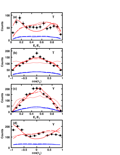
Figure 8: As for Fig. 6, but now the correlations are associated with the first step of ⁸C_g.s. decay forming 2p+⁶Be_g.s..

IV.2 ⁷B levels

The ⁷B excitation-energy spectrum determined from all detected 3p+$\alpha$ events is displayed in Fig. 9(a). The peak near zero excitation energy indicates that the ground state of ⁷B was produced in the reaction. There is a significant contamination in this spectrum from ⁸C_g.s. disintegrations where only 3 of the 4 protons were detected. To determine the contribution from this process, we have taken detected 4p+$\alpha$ events associated with ⁸C_g.s. and generated pseudo 3p+$\alpha$ events by alternatively removing one of the protons and determined the ⁷B excitation energy. The distribution of these excitation energies is labeled as ⁸C_g.s. in Fig. 9(a) and indicates that the incompletely detected ⁸C_g.s. events lead to an enhancement of the low-energy side of the ⁷B_g.s. peak. The Monte Carlo simulations were used to normalize the ⁸C_g.s. distribution to the expected number of incomplete detected events. The data points in Fig. 9(b) show the results for the ⁷B excitation-energy spectrum after this ⁸C_g.s. contamination was subtracted.

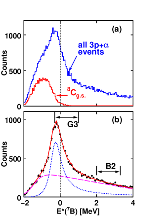
Figure 9: (Color online) (a) The excitation-energy spectra for ⁷B events determined from all detected 3p+$\alpha$ events and from ⁸C_g.s. 4p+$\alpha$ events where one of the protons was ignored. (b) The data points are the ⁷B excitation-energy spectrum after the ⁸C contamination was subtracted. The solid curve shows a fit to this data assuming an R-matrix line shape and including the detector response. The long-dashed curves indicate the background obtained from the fit and the raw R-matrix line shape is indicated by the dotted curve.

The subtracted distribution peaks at $E^{*}\sim$-100 keV rather than zero, suggesting that the evaluated mass excess from Ref. Audi03 used to calculate the Q value for this figure is incorrect. This evaluated mass excess of 27.94$\pm$0.10 MeV was derived from an average of two measurements; 27.80$\pm$0.10 MeV from the ⁷Li($\pi^{+}$,$\pi^{-}$)⁷B reaction and 27.94$\pm$0.10 MeV from the ¹⁰B(³He,⁶He)⁷B reaction McGrath67 .

As this is a rather wide level near threshold, the use of a Breit-Wigner line shape may not be appropriate. We have used R-matrix theory Lane58 assuming p+⁶Be_g.s. as the only open decay channel. The line shape is given by Eq. (8) where now $E_{x}$ is the energy above the p+⁶Be_g.s. threshold, and $Q_{2}$ is the resonance energy. Using $J^{\pi}$=3/2^- listed in the ENSDF database and $\ell$=1, the experimental spectrum was fit by adjusting $E_{2}$ and $\gamma_{2}^{2}$ and other parameters defining a smooth background under the peak. The effects of the detector acceptance and resolution was taken into account via the Monte Carlo simulations. The resulting fit is displayed as the solid curve in Fig. 9(b) and the fitted background is shown as the dashed curve. The dotted curve shows the fitted peak shape without the effects of the detector acceptance and resolution.

The fitted resonance energy is $Q_{2}$=2.013$\pm$0.025 MeV which implies a mass excess of 27.677$\pm$0.025 MeV. The error includes the effect in a 20% uncertainty in the magnitude of the subtracted ⁸C contamination. This mass excess is consistent with the previous measurement from the ⁷Li($\pi^{+}$,$\pi^{-}$)⁷B reaction, but is inconsistent with that from the ¹⁰B(³He,⁶He)⁷B reaction. The fitted reduced width is $\gamma_{2}^{2}$=1.32$\pm$0.02 MeV and thus the level widthLane58 ,

$$\Gamma^{0}=\frac{\Gamma(Q_{2})}{1+\gamma_{2}^{2}\,\frac{dS_{\ell}}{dE_{x}}\big{)}_{E_{x}=Q_{2}}},$$ (21)

is 0.80$\pm$0.02 MeV. The evaluated width in the ENDSF database is 1.4$\pm$0.2 MeV derived from the ¹⁰B(³He,⁶He)⁷B reaction McGrath67 . Again our results are inconsistent with this measurement.

In the above analysis of this level, we assumed ⁷B${}_{g.s.}\rightarrow$ p+⁶Be_g.s. sequential decay. We can check this by looking for a ⁶Be_g.s. fragment as described in Sec. IV.1. Here, there are only three ways to reconstruct a ⁶Be fragment from 3 protons and an $\alpha$ particle. The distribution of all three possible ⁶Be excitation energies is shown in Fig. 4(b) for the gate $G3$ in Fig. 9(b) on the ⁷B excitation energy. This gate does not cover the whole of the ⁷B_g.s. peak width, but avoids the lower energies where the ⁸C contamination is present. The ⁶Be excitation-energy spectrum displays a prominent peak at zero excitation energy indicating that ⁶Be_g.s. fragments were produced in the decay. The solid curve shows a fit to the data using the experimental ⁶Be_g.s. line shape [Fig. 2(b)] and a smooth Gaussian background (dashed curve) under this peak. From this fit we determine that, on average, there is a 54$\pm$6% probability of finding a ⁶Be_g.s. fragment in the $G3$ gate. However it is clear from Fig. 9(b) that there is a very significant background under this peak. Using gate $B2$ in Fig. 9(b) we estimate that the background has a 19$\pm$2% probability of containing a ⁶Be_g.s. fragment. Using this, we find that 81$\pm$10% of the ⁷B_g.s. events decay via p+⁶Be_g.s..

Shell-Model calculations for ⁷B_g.s. with the CKI Hamiltonian Cohen65 ; *Cohen67 give the spectroscopic factor for the p+⁶Be configuration as $S$=0.59(7/6) = 0.688. The p+⁶Be_1.67(2⁺) configuration is predicted to be $\sim$3 times stronger but decay to this channel is suppressed due to its significantly smaller barrier penetration factor. With $\theta^{2}_{sp}$=0.688 from Eq. (15), this gives us a predicted reduced width of 1.42 MeV [Eq. (16)]. Taking into account the 81% branching ratio, we estimate the experimental value to be $\gamma^{2}$=1.07$\pm$0.15 MeV which is quite similar to the predicted value confirming that the p+⁶B_g.s. is not the strongest configuration in ⁷B_g.s..

Although it is possible to consider a proton decay through the 1.670-MeV ($J^{\pi}$=2⁺) first-excited state of ⁶Be (see Fig. 3), this ⁶Be intermediate state is sufficiently wide that the disintegration is democratic. The average energy released in the first step is $E_{k}$=343 keV (determined from the differences in centroids of the two levels) which is very small compared to the width of the intermediate state, $\Gamma$=1.16 MeV. Alternatively, the distance traveled by the proton on average before the ⁶Be fragment decays is 2.0 fm which is small compared to the nuclear diameter. Thus this decay strength is probably best described as a 4-body decay.

IV.3 ⁸B levels

The ⁸B excited states studied in this work and their observed decay paths are illustrated in the level diagram of Fig. 10. We observed excited states in three detected exit channels; p+³He+$\alpha$, 2p+⁶Li, and 2p+d+$\alpha$. The p+⁷Be channel, which is probably the most important exit channel for many states, was not accessible in this work as Be fragments saturate the Si shaping amplifiers.

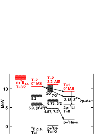
Figure 10: (Color online) Level scheme showing the levels of ⁸B discussed in this work and their decay paths.

IV.3.1 p+³He+$\alpha$ exit channel

The ⁸B excitation-energy spectrum derived from all detected p+³He+$\alpha$ events, shown in Fig. 11(a), displays wide peaks at 5.93 and 8.15 MeV. The ⁷Be excitation-energy distribution obtained from the ³He+$\alpha$ pairs associated with each of these events is shown in Fig. 11(b). A peak associated with the 4.57-MeV 7/2^- level is prominent. The total ⁸B excitation spectra is subdivided in Fig. 11(a) into those in coincidence with the ⁷Be peak [gate $G4$ in Fig. 11(b)] and those that are not. This subdivision separates the two ⁸B peaks. The 5.93-MeV peak is associated with proton decay to the 4.57-MeV state of ⁷Be and 8.15-MeV state does not decay by this path. Let us first concentrate on the 5.93-MeV peak.

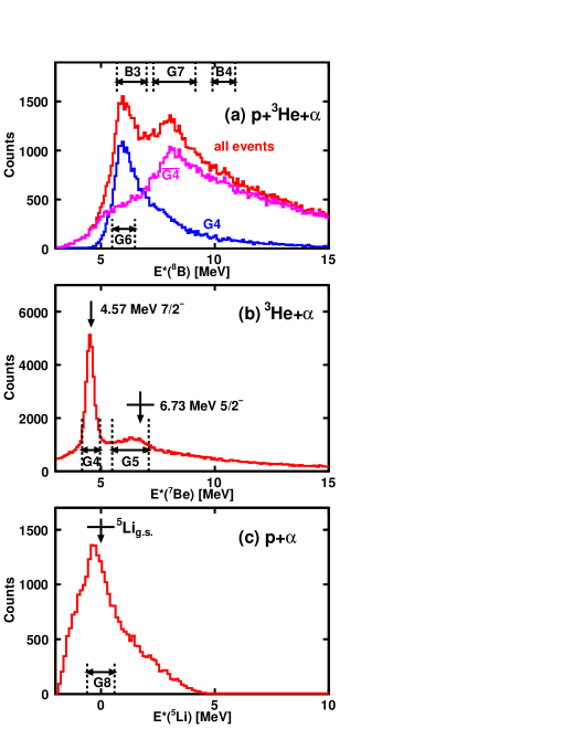
Figure 11: (Color online) Excitation-energy spectra determined from p+³He+$\alpha$ events. (a) The ⁸B excitation spectrum from all p+³He+$\alpha$ events and its decomposition into those associated with the 4.57-MeV ⁷Be intermediate state and those not. (b) The ⁷Be excitation spectrum obtained from the ³He-$\alpha$ pairs of all p+³He+$\alpha$ events. (c) Background-subtracted ⁵Li excitation-energy spectrum associated with the 8.15-MeV state in ⁸B. Vertical arrows locate known levels with their widths indicated by the error bars. The gates used in this work are also indicated by the dashed lines.

As there are only three fragments in the exit channel, the velocity vectors of the decay products are located in a plane in the ⁸B center-of-mass frame. To display the correlations between the decay fragments, we have projected these vectors onto that plane, and then within this plane, rotated all the vectors such that the locations of all the $\alpha$-particle velocities approximately coincide and at the same time the locations of all the ³He fragments velocities approximately coincide. This was achieved by requiring that the relative ³He-$\alpha$ velocity was parallel to the $V_{z}$ axis. A contour plot of the resulting distribution of p, ³He, and $\alpha$ velocities is displayed in Fig. 12. The ³He-$\alpha$ separation is constant as these fragments come from the decay of the 4.57-MeV ⁷Be state. The protons lie approximately on an arc centered at the origin (⁸B center of mass) as indicated by the dashed curve. Clearly the protons were emitted in the first step and the magnitude of their velocity is independent of their emission direction and the subsequent decay axis of the ⁷Be intermediate state.

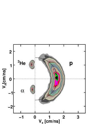
Figure 12: (Color online) Distributions of velocities of the three fragments for the p+³He+$\alpha$ exit channel associated with the 5.93-MeV ⁸B state. Events were selected using the $G4$ and $G6$ gates in Fig. 11. The distributions are projected onto the plane of the decay, with all ³He and all $\alpha$-particles locations forced to be approximately coincident.

The decay of this state is expected to be sequential with $R_{E}$=0.11 and $d_{E}$=60 fm, and thus the two decay steps are largely independent, apart from consideration of conservation laws. Angular momentum conservation gives rise to the angular correlations. Let us consider the relative angle $\theta_{12}$ between the two decay steps which is related to the angle $\theta_{k}$ in the Jacobi “Y” system. A $\theta_{12}$=0 corresponds to an event where the proton in the first step and the $\alpha$ in the second step are emitted in the same direction. The distribution of $\theta_{12}$ is shown as the data points in both panels of Fig. 13. The experimental distribution is symmetric about $\cos(\theta_{12})$=0 consistent with the expectation for a sequential decay scenario. The experimental distribution is clearly not isotropic (flat). The predicted correlations in a sequential decay depend of the initial spin $J$ and the total angular momentum removed by the proton $j_{p}$ in the first decay step. The predicted correlations do not depend on the parity of the initial state for these proton decays, but mixing between $j_{p}$ values should also considered, i.e., the angular correlation becomes

$$w(\theta_{12}) = \left|\alpha_{1}\right|^{2}w_{1}(\theta_{12})+\left|\alpha_{2}\right|^{2}w_{2}(\theta_{12})$$ (22)

$$+(\alpha_{1}\alpha_{2}^{*}+\alpha_{1}^{*}\alpha_{2})w_{inter}(\theta_{12}),$$

where $w_{1}$ and $w_{2}$ are the correlations associated with two pure values of $j_{p}$, $\alpha_{1}$ and $\alpha_{2}$ are their complex amplitudes and $w_{inter}$ is the interference term.

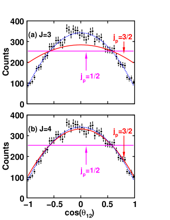
Figure 13: (Color online) Angular correlations for the 5.93-MeV state of ⁸B. Events were selected using both the $G4$ and $G6$ gates in Fig. 11. The angle $\theta_{12}$ in the relative angle between the initial proton decay axis and the subsequent ³He-$\alpha$ decay axis in the ⁸B center-of-mass frame. The proton and $\alpha$ particle are emitted in the same direction when $\theta_{12}$=0. The solid curves are predictions for pure values of $j_{p}$, while the dashed curves are for mixed values where the degree of mixing was chosen to best fit the data.

With this mixing, only two possible $J$ values were consistent with the experimental distributions. Figure 13(a) shows the results for $J$=3. The two solid curves show the predictions for two pure values of $j_{p}$; 1/2 and 3/2. These predictions have been normalized to the same number of events as in the experimental distribution and Monte Carlo simulations indicate that the distortions due to the angular acceptance and energy resolution of the detectors are minimal. Neither of these predictions fit the data at all. However, a mixed solution with relative amplitudes of $\alpha_{1}$=1 and $\alpha_{2}$=0.49$\pm$0.14 for the two $j_{p}$ values, respectively, fits the data very well [dashed curve in Fig. 13(a)].

The other solution was obtained for $J$=4 and is shown in Fig. 13(b). Again, pure $j_{p}$=1/2 and 3/2 predictions are shown by the solid curves. In this case the $j_{p}$=3/2 predictions fits the data reasonably well. If we allow for mixing, the best fit is obtained with relative amplitudes of $\alpha_{2}$=1 and $\alpha_{1}$=-0.07$\pm$0.10, however, the level of mixing is minimal. All told, the angular correlations indicate that the 5.91-MeV state is either $J$=3 or 4.

For the 8.15 MeV state in ⁸B, which does not proton decay to the 4.57-MeV ⁷Be state [Fig. 11(a)], it is difficult to clearly define its decay path due to the larger background under this peak and also because there are no possible narrow intermediate states through which it can decay. Sequential decay through a higher-lying ⁷Be state and through the ⁵Li ground state are possible. Apart from the narrow 4.57-MeV state, the ⁷Be excitation spectra in Fig. 11(b) shows a broad peak at $\sim$6.5 MeV, close to the location of the $E^{*}$=6.73-MeV, $J^{\pi}$=5/2^-, $\Gamma$=1.2-MeV state in ⁷Be, indicated by the arrow in the Fig. 11(b). For a wide intermediate state, the full width of the state is not always populated by sequential decay as the Coulomb barrier of the first step can suppress the higher excitation region. The peak at 6.5 MeV may be associated with the 6.73-MeV state and gating of this peak enhances the 8.15-MeV peak. However for all the p+³He+$\alpha$ events, only 30$\pm$6% of the kinetic energy, in the reconstructed ⁸B frame, is associated with the proton. Thus the ³He+$\alpha$ pair accounts for the remaining 70$\pm$6% and thus the ³He-$\alpha$ reconstructed excitation energy is strongly correlated to p+³He+$\alpha$ excitation energy suggesting that the 6.5-MeV peak in ⁷Be spectra in Fig. 11(b) is a reflection of the peak at 8.15 MeV in Fig. 11(a) due to this strong correlation and not associated with an intermediate state.

Also possible is the decay ⁸B${}^{*}\rightarrow^{3}$He+⁵Li_g.s. Figure 11(c) shows the reconstructed ⁵Li excitation-energy spectrum determined for the p-$\alpha$ pairs associated with the 8.15-MeV peak [gate $G7$ in Fig. 11(a)]). A rough background correction was made using gates $B3$ and $B4$ on either side of the 8.15-MeV peak. A broad peak at zero excitation energy is observed overlapping strongly with the ground state of ⁵Li. Angular correlations were constructed for both the two sequential decay scenarios, and after background subtractions, are shown in Fig. 14. In this figure $\theta_{12}$=0 for ³He+⁵Li_g.s. decay corresponds to the ³He and $\alpha$ being emitted in the same direction. The ³He-⁵Li_g.s. results is clearly asymmetric about $\cos(\theta_{12})$=0 and cannot be explained by sequential decay. For the p+⁷Be_6.73 case, although the distribution is symmetric about $\cos(\theta_{12})$=0, we were unable to fit it with the range of possible correlations expected for a 5/2^- intermediate state and thus there is no evidence for a sequential decay of this state which suggets the decay is 3-body in nature.

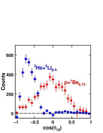
Figure 14: (Color online) Background-subtracted angular correlations associated with possible sequential-decay scenarios for the 8.15-MeV state of ⁸B. The 8-15-MeV peak was selected with gate $G7$ in Fig. 11 and the background was estimated from $B3\cup B4$. For proton decay to the 6.73-MeV state of ⁷Be, the extra gate $G5$ was applied and for ³He decay to the ground state of ⁵Li, the extra gate $G8$ was applied.

IV.3.2 2p+⁶Li exit channel

The excitation-energy spectrum derived from 2p+⁶Li events in Fig. 15 displays a very prominent peak at 7.06$\pm$0.02 MeV. The excitation energy in Fig. 15 was calculated based on the assumption that the ⁶Li fragments were created in their ground states and did not $\gamma$ decay. Only one ⁶Li excited state has a significant $\gamma$-decay branch, the 3.562-MeV, $J^{\pi}$=0⁺, $T$=1 level whose $\gamma$ branching ratio is practically 100%. Therefore the peak observed in Fig. 15 can correspond to a level of excitation energy of either 7.06$\pm$0.02 or 10.62$\pm$0.02 MeV.

The intrinsic width of this level is quite narrow as the experimental width is similar to the predicted instrumental resolution. If we assume a Breit-Wigner line shape, we can further constrain the width. The curves in Fig. 15 show Monte Carlo predictions including the detector response for intrinsic widths of 50, 75, and 100 keV normalized to the experimental peak height. The behavior in the region of the low-energy tail, where the uncertainty due to the background contribution is minimal, suggests an intrinsic width of less than 75 keV.

There are no previously known levels at $E^{*}$=7.06 MeV. From the mirror nucleus ⁸Li, we expect only one narrow state near this energy, the mirror of the 6.53-MeV $J^{\pi}$=4⁺, $\Gamma$=35 keV level. However, this ⁸Li state has a significant branch to the n+t+$\alpha$ exit channel passing through the 4.63-MeV ⁷Li Grigorenko02 . As the 7.06-MeV state is not observed is the mirror exit channel p+³He+$\alpha$ (see Fig. 11) is seems unlikely that it can be this $J^{\pi}$=4⁺ state.

On the other hand, if the peak in Fig. 15 corresponds to a 10.62-MeV state, then we can immediately identify it with the known 10.619$\pm$0.009 MeV $J^{\pi}$=0⁺ $T$=2 state in ⁸B with $\Gamma<$60 keV Robertson75 . The almost exact matching of the excitation energy and a consistent limit to the width strongly support this assignment.

With this assignment, the ⁸B state is thus the isobaric analog of ⁸C_g.s. discussed in Sec. IV.1 and its structure should be similar. It decays by the emission of two protons to the isobaric analog of ⁶Be_g.s. in ⁶Li. Such a decay can conserve isospin only if the two protons are emitted promptly in a $T$=1 configuration. Sequential two-proton decay does not conserve isospin as there are no energetically accessible $T$=3/2 states available in the ⁷Be intermediate nucleus (see Fig. 10). This is an isospin equivalent to the Goldansky two-proton decay, as the isospin allowed intermediate state is energetically forbidden.

Further elucidation of the nature of this two-proton decay may be obtained from the correlations between the fragments. Unfortunately in this experiment, most ⁶Li fragments were not identified due to a saturation of the Si amplifiers, thus most of the 2p+⁶Li events associated with this state were not observed except where the ⁶Li fragment had high kinetic energy (low $\Delta E$) strongly biasing any correlation measurement. A future experiment is planned to study this correlation.

Figure 15: (Color online) Excitation-energy spectra from 2p+⁶Li events. The curves show simulated distributions for Breit-Wigner line shapes with the indicated decay widths. The lower curve below the data, indicates the background which was included in the simulated distributions.

IV.3.3 2p+d+$\alpha$ exit channel

The ⁸B isobaric analog state also decays to the 2p+d+$\alpha$ exit channel. Here, the decay is isospin forbidden and the yield is much smaller than that obtained for the 2p+⁶Li channel (Table 1), further suggesting that the latter is an isospin-allowed decay. The excitation-energy spectrum extracted from these events is plotted in Fig. 16(a) and shows a narrow peak at the energy of the isobaric analog state (arrow). Possible narrow intermediate states are the ⁶Be ground state and the 2.18-MeV $J^{\pi}$=3^{+ 6}Li excited state, although we found no evidence that the former is associated with this peak and in fact used the ⁶Be ground state as a veto to reduce the background. The background was also reduced by gating on the reconstructed ⁸B velocity distribution associated with the IAS peak for the 2p+⁶Li events. The spectrum labeled “all events” contained these two background reducing gates. For “all events”, the reconstructed ⁶Li excitation spectra from the d-$\alpha$ pairs is shown in Fig. 16(b) where the 2.18-MeV state is quite prominent. Gating on this state [gate $G4$ in Fig. 11(b)], produces the excitation-energy spectrum shown in Fig. 16(a). The peak in this case contains only $\sim$50% of the strength of the “all events” peak. The origin of the remaining strength is not clear, possibly from 3 or 4-body decays, but certainly is not associated with sequential decay through a narrow state.

For the strength associated with the 2.18-MeV ⁶Li state, we were not able to identify any ⁷Be intermediate levels. Either the two protons are emitted in an initial 3-body decay or the ⁷Be intermediate state(s) are too wide to isolate experimentally. Because of the low yields, the statistical errors associated with the background-subtracted correlations are too large to extract any further information.

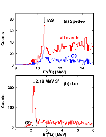
Figure 16: (Color online) (a) ⁸B excitation-energy spectra obtained from 2p+d+$\alpha$ events. (b) ⁶Li excitation-energy spectrum obtained from each d-$\alpha$ pair of each 2p+d+$\alpha$ event. The arrows indicate the locations of known states. The gate $G9$ in (b) is used to gate the spectrum in (a).

IV.4 ⁸Be levels

A high lying ⁸Be state is seen in the p+t+$\alpha$ excitation spectrum. The distribution from all detected events is displayed in Fig. 17(a)(“all events”). A broad peak is observed at 22.96 MeV. Such a peak was also observed previously following the fragmentation of a ¹²Be beam and was associated with proton decay to the 4.63-MeV $J^{\pi}$=7/2^{- 7}Li excited state Charity08 . This is confirmed in the present work. The excitation spectrum obtained from the t-$\alpha$ pairs is shown in Fig. 17(b) where the 4.63-MeV ⁷Li state is quite prominent. Gating on this peak [gate $G10$ in Fig. 17(b)] produced the “$G10$” spectrum in Fig. 17(a). The gate significantly reduced the background, but did not reduce the yield in the peak indicating that proton decay to the 4.63-MeV state is the dominant decay mode.

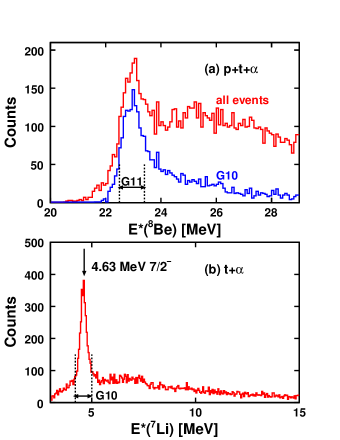
Figure 17: (Color online) (a) ⁸Be excitation-energy spectra from p+t+$\alpha$ events. (b)⁷Li excitation-energy spectrum from the t-$\alpha$ pairs in each p+t+$\alpha$ event.

This state has similarities to the 5.93-MeV state in ⁸B which proton decays to the 4.57-MeV state in ⁷Be, i.e., the mirror state to the 4.63-MeV in ⁷Li. Figure 18 compares the angular distributions of $\theta_{12}$ in the decay of these two states. Here the ⁷B data were scaled to the same number of total counts as the ⁷Be results. Within the statistical errors, the correlations are identical suggesting that the 22.96-MeV state in ⁸Be is the analog of the 5.93-MeV ⁸B state and thus would have the same possible spin assignments ($J$=3 or 4 ). The intrinsic widths of these two states are also comparable; 850$\pm$260 and 680$\pm$146 keV for ⁸B and ⁸Be, respectively.

In Fig. 19 we show these levels in an isobar diagram of $T$=1 levels. The relative excitation energies of these two levels is also consistent with their assignment to the same isospin triplet. The corresponding analog in the ⁸Li nucleus is not entirely clear. A 6.1-MeV ⁸Li state with $\Gamma\sim$1 MeV is a possibility; it has been tentatively assigned $J$=3.

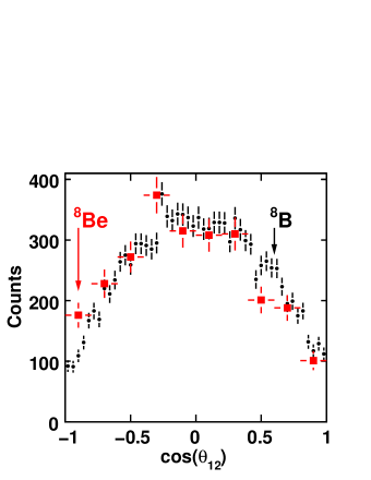
Figure 18: (Color online) Comparison of angular correlations obtained for the 5.92-MeV state in ⁸B and the 22.96-MeV state in ⁸Be. The correlations for the ⁸Be state were obtained using gates $G10$ and $G11$ in Fig. 17.

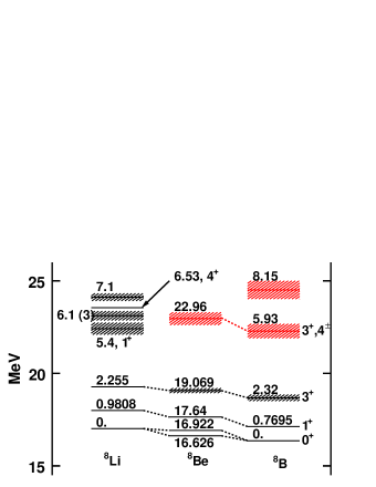
Figure 19: (Color online) Isobar level diagram of $T$=1 states for $A$=8. The levels discussed in this work are displayed in red. The energy scale on the y axis is with respect to the ⁸Be ground state.

IV.5 ⁹B

We observed ⁹B levels in the p+2$\alpha$ and 2p+⁷Li exit channels. Figure 20 shows a level diagram with the levels of interest and their decay paths.

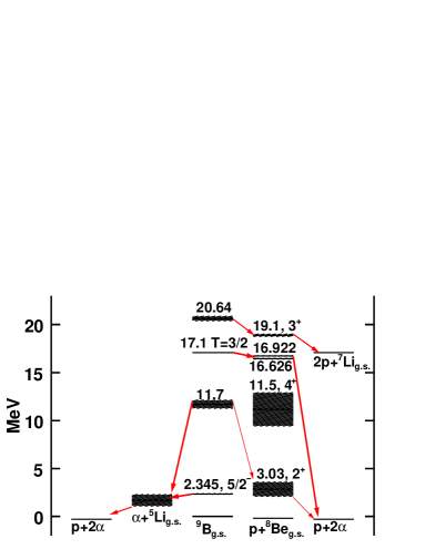
Figure 20: (Color online) Level diagram for ⁹B showing the levels discussed in this work and their decay paths. The energy scale on the y axis is with respect to the ⁹B ground state.

IV.5.1 p+2$\alpha$ exit channel

The ⁹B excitation-energy spectrum derived from p+2$\alpha$ events, displayed in Fig. 21(a), shows many peaks. The most prominent of these are the ground state and the 2.345-MeV $J^{\pi}$=5/2^- level. The spectrum above these two peaks has been scaled by a factor of three to show additional detail. Prominent peaks are also observed at 11.7 and 14.7 MeV. For the latter, two listed levels can contribute, the narrow 14.655-MeV isobaric analog state and the wider 14.70-MeV ($\Gamma$=1.35 MeV) state. Judging by the shape of the 14.7-MeV peak, it is likely that both levels are present. As it is impossible to separate the decay modes of these two levels, we will not report on any further analysis of this peak.

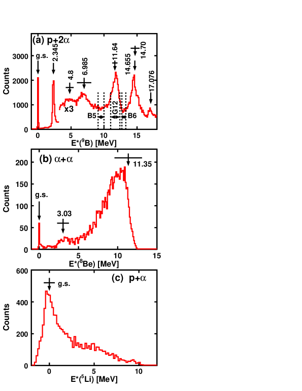
Figure 21: (Color online) (a) Excitation-energy spectra of ⁹B derived from p+2$\alpha$ events. (b) The ⁸Be excitation-energy spectra obtained from the $\alpha$-$\alpha$ pairs for events in the 11.7-MeV ⁹B ($G12$ gate), (c) Background subtracted ⁵Li excitation-energy spectra for events in the 11.7-MeV ⁹B peak. The arrows indicate the locations of known levels.

The peak at 11.7 MeV is close to a listed 11.640-MeV level with a tentative spin assignment of $J^{\pi}$=7/2^-. The width of this listed level (780$\pm$45 keV) is also close to the value of 880$\pm$80keV extracted from the peak after correction for the experimental resolution. For further analysis of the correlations associated with this peak, we use the gate $G12$ in Fig. 21(a) with the regions $B5$ and $B6$ on either side to estimate the background under the peak. The ⁸Be excitation-energy spectra from the $\alpha$-$\alpha$ pairs associated with each event in the $G12$ gate is plotted in Fig. 21(b). The “background” was not subtracted from this spectrum as the reconstructed ⁸Be ($\alpha$+$\alpha$) and ⁹B (p+$\alpha$+$\alpha$) excitation energies are highly correlated. This is similar to the strong correlation between the ³He+$\alpha$ and p+³He+$\alpha$ reconstructed excitation energies found in Sec. IV.3.1. Due to this correlation, the spectra from gates $B5$ and $B6$ are not good approximations to the background associated with gate $G12$ for the ⁸Be excitation energy. In Fig. 21(b), contributions from the ⁸Be ground state and the 3.03-MeV first excited state are clearly present. However, the ground-state contribution is essentially all background because when we gate on this peak and project the ⁹B excitation-energy distribution, no indication of the 11.7-MeV peak is seen. On the other hand, the 3.03 MeV peak is not all background. With a similar gating arrangement, we find $\sim$2.8% of the strength at 11.7 MeV is be associated with this ⁸Be intermediate state.

Most of the 11.7-MeV ⁹B peak is thus associated with the broad structure above $E^{*}(^{8}Be)$=5 MeV in Fig. 21(b). This structure overlaps with the wide 11.35-MeV $J^{\pi}$=4^{+ 8}Be level. The situation here is similar to the 8.15-MeV ⁸B state. The centroid of the structure in Fig. 21(b) is below the centroid for this level, possibly a consequence of sequential feeding. However the ⁸Be and ⁹B excitation energies are well correlated and thus the structure could just be a consequence of this correlation. The alternative intermediate state is ⁵Li. Fig. 21(c) shows the background-subtracted ⁵Li excitation-energy spectrum associated with the 11.7-MeV peak obtained from the p+$\alpha$ pairs. There are two possible p+$\alpha$ pairs from each p+2$\alpha$ event and both are included in this spectrum. A peak corresponding to the ground state of ⁵Li is clearly present indicating that $\alpha$+⁵Li_g.s. is an important decay branch.

The correlations associated with the decay of the 11.7-MeV state can be displayed in a manner similar to Fig. 12 where we projected the velocity vectors onto the decay plane. To localized the distribution of $\alpha$ particles, the $\alpha$-$\alpha$ relative velocity was made parallel to the $V_{z}$ axis, and as we cannot distinguish the two $\alpha$ particles, we have symmetrized the distributions about $V_{z}$=0. The velocity plot for the 11.7-MeV state is displayed in Fig. 22(a) and can be compared to the corresponding plot for the 2.345-MeV state in Fig. 22(c). Unlike Fig. 12 where the protons lie on an arc centered at the origin, the protons in Fig. 22(a) lie on two overlapping arcs each centered approximately near an $\alpha$ particle. These two arcs indicate that the protons are not emitted from the ⁹B center of mass, as expected for direct proton decay, but come predominantly from the decay of a ⁵Li intermediate fragment. Thus the broad peak in the $\alpha$-$\alpha$ excitation spectrum in Fig. 21(b) should not be interpreted as an ⁸Be excited state.

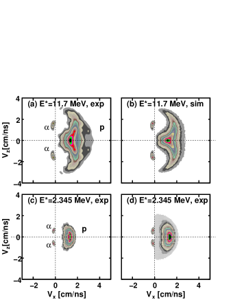
Figure 22: (Color online) Distributions of the velocities of the three fragments for the p+2$\alpha$ exit channel associated with (a,b) the 11.7-MeV and (c,d) the 2.345-MeV states of ⁹B. The distributions are projected on the plane of the decay with the two $\alpha$-particle velocities localized. The experimental distributions in (a,c) are compared to simulated distributions for $\alpha$-⁵Li_g.s. decay in (b,d).

The distributions in Figs. 22(b) and 22(d) show the results of simulations of a sequential disintegration initiated by an $\alpha$+⁵Li_g.s. decay. The 2.345-MeV level was previously identified as having strong $\alpha$+⁵Li_g.s. decay character Charity07 , however the two arcs are not separated as the two $\alpha$ particles are located too close together. In both simulations we have determined the emission energies in the two steps using the R-matrix formalism as described in Sec. III. Both simulations reproduce the experimental distribution reasonably well.

Information about the spin of the 11.7-MeV state can be determined from the angular correlations of the two decay steps. Unfortunately as the two arcs overlap, we cannot always identify which $\alpha$ particle is emitted in the first and second steps and thus we cannot uniquely determine $\theta_{12}$. Instead we have looked at the angle $\theta_{2\alpha-p}$ defined in Fig. 23. This is the angle between the relative velocity vectors of the two $\alpha$ particles ($V_{\alpha-\alpha}$) and the proton velocity ($V_{p}$) in the ⁹B center-of-mass frame. Background-subtracted distributions of this quantity are shown for both the 11.7 and 2.345-MeV states in Fig. 24. For an initial $\alpha$-particle decay, unlike proton decay, the angular correlations are sensitive to the parity of the initial level. Furthermore if we constrain ourselves to $\alpha$ decays with the lowest possible $\ell$ waves, there is no mixing to consider and each $J^{\pi}$ value has a unique correlation. The prediction obtained for the 2.345-MeV level with its known spin of 5/2^- is compared to the experimental data in Fig. 24(b). It fits the data extremely well and thus again is consistent with sequential decay initiated by an $\alpha$-⁵Li_g.s. decay. In Fig. 24(a) for the 11.7-MeV state, we show three predictions which fit the experimental data with $J^{\pi}$=3/2^-, 5/2⁺, and 7/2^-. Of these, the 3/2^- predictions gives the best fit with a $\chi^{2}/\nu$=1.7. The other two cases have $\chi^{2}/\nu$=2.6 and 3.0 respectively, so $J^{\pi}$=3/2^- is slightly preferred. We note, that the listed 11.64-MeV state in ⁹B has a tentative assignment as $J^{\pi}$=7/2^- which is the least likely of our three possible fits.

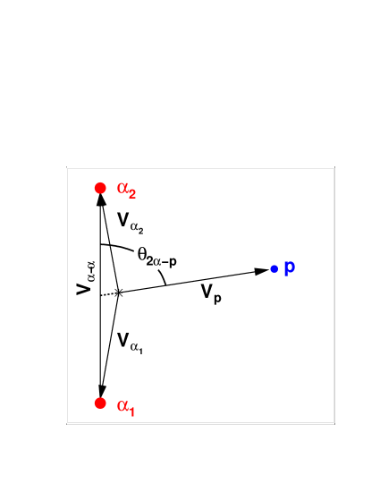
Figure 23: (Color online) Schematic showing the definition of the angle $\theta_{2\alpha-p}$.

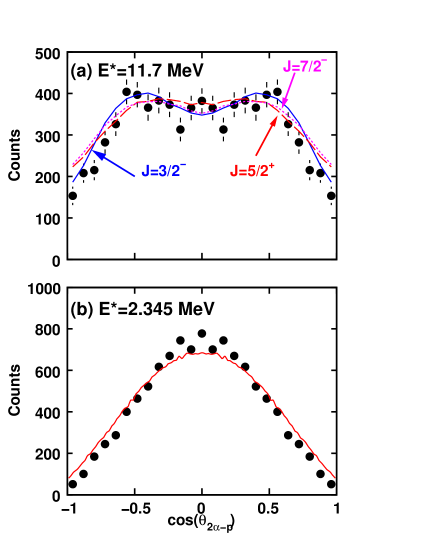
Figure 24: (Color online) Background-subtracted angular corrections measured in the decay of the (a) 11.7-MeV and (b) the 2.345-MeV states of ⁹B. The curves indicate calculated distributions assuming an initial $\alpha$-⁵Li_g.s. decay. In (a), the calculated results are given for a number of assumed spins for the 11.7-MeV state.

Figure 25 shows the energy correlations for the 11.7 and 2.345-MeV states in ⁹B. The correlations are presented in the Jacobi “Y” system where the “core” in Fig. 5 is now the proton and the “protons” in that figure are the $\alpha$ particles. The quantity $E_{x}$ is now the relative kinetic energy in the p-$\alpha$ subsystem and, for each event, the spectra are incremented twice, once for each the two p-$\alpha$ pairs. The curves are the R-matrix predictions using parameters for the ⁵Li_g.s. resonance from Ref. Woods88 . These sequential calculations reproduce the data quite well, further indicating a sequential character to these decays. The strong peak associated with the ⁵Li ground state is clearly resolved in Fig. 25(a) for the 11.7 MeV state.

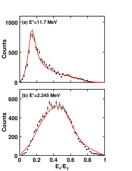
Figure 25: (Color online) Background-subtracted energy corrections in the Jacobi “Y” system measured in the decay of the (a) 11.7-MeV and (b) the 2.345-MeV states of ⁹B. The curves indicate calculated distributions assuming $\alpha$-⁵Li_g.s. decay in the R-matrix approximation.

The discussion of these ⁹B decays has ignored interactions between the two decay steps. For the 11.7-MeV level, the short life time of the ⁵Li_g.s. intermediate state is partially ameliorated by the large kinetic energy released in the first step ($E_{k}^{1}$=10 MeV). With this value we obtain $R_{E}$= 0.12 and $d_{E}$=16 fm for this decay. The products from the first step thus are separated by $\sim$6 nuclear radii, on average, before the second steps occurs. It is clear that in this case we would expect the sequential character of the decay to largely survive final-state interactions between the final fragments.

The sequential character of the 2.345-MeV state is more surprising. Here $E_{k}^{1}$ is much smaller and $R_{E}$=1.88 and $d_{E}$=4.0 fm and this should be a democratic decay. The value of $d_{E}$ is in fact one of the smallest values found in this work, even smaller than the value of 6.5 fm obtained for ⁶Be_g.s. decay.

Why does this state have such a strong sequential character, when ⁶Be_g.s. decay displays very little? Specifically we find that the angular correlations associated with sequential decay are found for the 2.345-MeV ⁹B state, but not for the ⁶Be_g.s.. A possible reason is that the ⁶Be_g.s. decay is approaching a Goldansky decay; most of the strength of the intermediate state is energetically inaccessible, whereas all the ⁵Li_g.s. strength is accessible for the 2.345-MeV state. Another consideration is that final state interactions between the products would be largest for $\cos(\theta_{2\alpha-p})$=$\pm$1, i.e., when one of the fragments from the second step is directed directly towards the $\alpha$ particle from the first step. However, the angular corrections are minimal for these cases and so the effect of final state interactions will also be minimized. Although the correlations do maintain a strong sequential character, the magnitude of the decay width cannot be explained from a R-matrix calculation (Sec. III). The R-matrix prediction by Barker was a factor of 4 too small Barker03a indicating the need for a three-body calculation.

One can also look for ⁹B levels which decay predominantly to ⁸Be states. The reconstructed ⁸Be excitation-energy spectrum from the $\alpha$-$\alpha$ pairs of each p+2$\alpha$ event is shown in Fig. 26(a). The ⁸Be ground state and a number of excited states indicated by the arrows are clearly present. The peak at $\sim$1.5 MeV is not a ⁸Be excited state, but rather is associated with the decay of the 2.345-MeV ⁹B excited state. Of particular interest is the strong peak associated with the 16.626 and 16.922-MeV mixed $T$=0+1 $J^{\pi}$=2⁺ states. These are narrow states, but the experimental resolution is not sufficient for their separation. The peak thus can contain contributions from both of these mixed-isospin states.

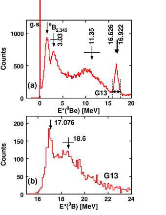
Figure 26: (Color online) (a) Excitation-energy distribution for ⁸Be fragments reconstructed from the $\alpha$-$\alpha$ pairs of all p+2$\alpha$ events. (b) The ⁹B excitation-energy distributions obtained with the $G13$ gate on the ⁸Be excitation energy.

The ⁹B excitation-energy spectrum obtained by gating of the $E^{*}\sim$17-MeV peak [gate $G13$ in Fig. 26(a)] is shown in Fig. 26(b). The peak at 16.99$\pm$0.04 MeV is clearly isolated although it was also present in the ungated spectrum of Fig. 21(a). This peak could correspond to a previously known level at 16.71$\pm$0.10 MeV or the 17.076$\pm$0.04-MeV $T$=3/2 level. Both decays satisfy isospin conservation and the former, if it has a significant d+⁷Be branching ratio, may be important in big-bang nucleosynthesis Chakraborty10 . The magnitude of the yield in the observed peak is consistent with that from the ungated spectrum in Fig. 21(a) indicating that this state predominantly decays to one or both of the ⁸Be $T$=0+1 levels. Presumably most of the decay is to the 16.626-MeV state as only the low-energy tail of the 16.922 MeV state is energetically accessible.

The 16.71-MeV level has only been observed before in one experimental study Dixit91 where it was suggested to be the mirror of the 16.67 MeV $J^{\pi}$=5/2⁺ state in ⁹Be. Experimental angular distributions in that work were consistent with this spin assignment. The spin of the 17.076-MeV state is not listed in the ENSDF database, however, it is probably the mirror of the 16.977-MeV $T$=3/2 ⁹Be state which has a spin of $J^{\pi}$=1/2^-. In the two cases we would thus expect the first step in the sequential decay would be dominated by $\ell$=0 and 1 decay, respectively, giving rise to different angular correlations.

We have extracted the angular correlation between the first proton emission step and the second 2$\alpha$ decay step for the events in the peak located at $\sim$17 MeV in Fig. 26(b). The higher-energy region directly adjacent in excitation energy was used for the background subtraction. The background-subtracted correlation is plotted in Fig. 27 and is compared to calculations for $J^{\pi}$=1/2^- ($\ell$=1) and $J^{\pi}$=5/2⁺ ($\ell$=0). Of these calculations, the data are in much better agreement with the $J^{\pi}$=1/2^- case, suggesting that the state observed is the $T$=3/2 state. The decay to the 16.626 MeV state is $R_{E}$=0.41 and $d_{E}$=45 fm, and the large value of the latter number suggests this is approaching a truly sequential decay.

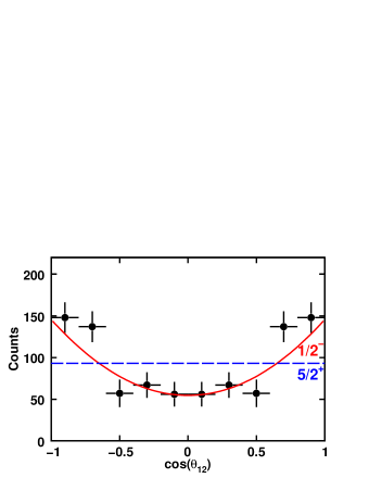
Figure 27: (Color online) Angular correlation for the 16.99 MeV state in ⁹B. Data points indicate the background-subtracted experimental results and the curves shows the results expected for the indicated level spins.

IV.5.2 2p+⁷Li exit channel

Due to the problem with the saturation of the amplifiers, only a small fraction of the ⁷Li fragments could be identified. However, there were sufficient statistics for the 2p+⁷Li exit channel to isolate a new level in ⁹B. The excitation-energy spectrum determined from 2p+⁷Li events is displayed in Fig. 28(a) and a peak at 20.64$\pm$0.10 MeV is evident with a width of $\Gamma$=450$\pm$250 keV. The large error is a consequence of an uncertainty of how to define the background when fitting this peak. We do not know whether the ⁷Li fragment was created in the ground state or the gamma-emitting 0.477-MeV excited state. The energy of the level could thus be either 20.64 or 21.12 MeV. We have attempted to see if the decay of this level could be associated with a sequential two-proton decay through a ⁸Be excited state. As there are two protons, we can reconstruct the two possible ⁸Be excitation energies from each 2p+⁷Li event. The background-subtracted distribution of both of these gated on the 20.64-MeV peak [gate G14 in Fig. 28(a) with background gates $B7$ and $B8$] is shown in Fig. 28(b). Again there is some uncertainty in the background subtraction, but the location of the peak was not affected by this. The peak can be identified with the 19.069 MeV, $\Gamma$=271 keV, $J^{\pi}$=3⁺ in ⁸Be. The curves in Fig. 28(b) show Monte Carlo simulations of the decay through this state. The long and short-dashed curves show the contributions from the correctly and incorrectly identified proton associated with ⁸Be decay, and the solid curve is the sum of these two. Both the correct and incorrect distributions have almost the same average energy, but the incorrect distribution is quite wide and the peak position is defined by the correctly identified proton which has a much narrower distribution. The simulation was performed assuming the second decay is to the ground state of ⁷Li. If we assumed the decay was to 0.477-MeV state, then the reconstructed ⁸Be peak energy would be at $\sim$19.5 MeV. No previously known ⁸Be excited state could be found at this energy but it is possible that decays occurs through an unknown ⁸Be excited state, however it seems more likely that the decay is to the ⁷Li ground state through the known 19.07-MeV state.

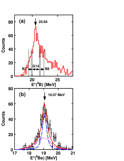
Figure 28: (Color online) (a) Excitation-energy distribution for ⁹B fragments reconstructed from 2p+⁷Li events. (b) The ⁸Be excitation-energy distributions obtained with the $G1$ gate on the ⁹Be excitation energy. The distributions contains contributions from both possible p-⁷Li combinations.

IV.6 ¹⁰C levels

Information on ¹⁰C states produced by neutron pickup and more complicated reactions was obtained from the 2p+2$\alpha$ exit channel. This is the only channel available for particle-decaying states with $E^{*}<$ 15 MeV. The excitation-energy spectrum from all of these events is displayed in Fig. 29(a) and is dominated by a peak at 9.69 MeV, although other smaller peaks are evident. In our previous work, levels for this exit channel were revealed by gating on the presence of various narrow intermediate states Charity09 . Figures 29(b), 29(c), and 29(d) show the ¹⁰C excitation-energy distribution gated on the ⁹B ground state, the ⁶Be ground state, and the 2.345-MeV ⁹B excited state, respectively.

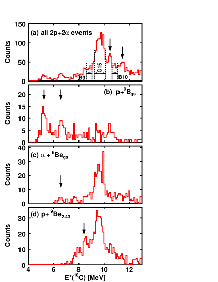
Figure 29: (Color online) Excitation-energy distributions for ¹⁰C fragments reconstructed from 2p+2$\alpha$ events. Panel (a) is for all events, while (b), (c) and (d) are gated on the presence of ⁹B_g.s., ⁶Be_g.s., and ⁹B_2.345 intermediate states. Arrows show the locations of the peaks discussed in this work. The gate $G15$ used to select the 9.69-MeV peak and the gates $B9$ and $B10$ used for background subtraction are indicted.

The arrows in Fig. 29(b) show the locations of two states (5.222 and 6.553 MeV) that were excited via the inelastic scattering of a ¹⁰C beam and which decay by proton emission to the ⁹B ground state Charity09 . These states dominated the total ¹⁰C excitation energy spectrum in inelastic scattering, but here they are weakly populated and require a gate by the ⁹B_g.s. to enhance them [see Fig. 29(b)]. As these states are expected to have 2$\alpha$ cluster structure Charity09 , then it is not surprising that a neutron-pickup by ⁹C (which does not have any 2$\alpha$ cluster structure) does not populate these states strongly.

The widths of these states also appear to be wider (by 50-70%) than we would expect based on the intrinsic widths given in Ref. Charity09 and the simulated experimental resolution. Possibly these peaks are actually doublets which would not be surprising as other levels near these energies are expected based on the mirror nucleus ⁹Be. At higher excitation energies in Fig. 29(b), there may also be indications of other states, though the statistical errors are large. We note the absence of any significant contribution from the 9.69-MeV level in this spectrum.

A 6.56-MeV state which decayed via the $\alpha$+⁶Be_g.s. channel was also observed in the inelastic excitation of a ¹⁰C beam Curtis08 ; *Curtis10; Charity09 . Its location is indicated by the arrow in Fig. 29(c). This state is also expected to have strong cluster structure and is clearly only weakly populated in the present experiment. In Fig. 29(c), the spectrum is again dominated by the 9.69-MeV peak, indicating that $\alpha$+⁶Be_g.s. is an important decay branch for this level.

The spectrum in Fig. 29(d) is also dominated by the 9.69-MeV level indicating that this level has a second decay branch (p+⁹B_2.345). Also a smaller peak appears at 8.5 MeV. The arrow in this figure shows the location of an 8.4 MeV state that was previously shown to decay through the 2.345-MeV ⁹B intermediate level. However, the intrinsic width of that state was $\sim$1 MeV, significantly wider than the present peak. The experimental width of the peak in this work ($\sim$300 keV) is consistent with the simulated resolution. Within the statistical uncertainties we estimate $\Gamma<$200 keV.

Other small peaks are also suggested in the total distribution in Fig. 29(a). The peaks at 10.48 and 11.44 MeV, indicated by the arrows in this figure, are previously unknown. Their widths are consistent with the experimental resolution. The decay of these states is not known; they do not feature prominently in the distributions gated by the long-live intermediates.

IV.6.1 9.69-MeV state

The strong 9.69-MeV state is wider than the other observed ¹⁰C states; from the simulation we estimate its intrinsic width is 490 keV. It was not observed via ¹⁰C inelastic scattering in Refs. Curtis08 ; *Curtis10; Charity09 suggesting that it does not have a strong cluster structure and maybe is more single-particle in nature. In any case we will show its decay modes are quite interesting. In the following we give an analysis of correlations associated with this peak using gate $G15$ and background gates $B9$ and $B10$ in Fig. 29(a). All the distributions discussed in the remainding of this section are background subtracted.

As we have observed in Fig. 29(c) and 29(d), the 9.69 MeV level has strength for decays into the $\alpha$+⁶Be_g.s. and p+⁹B_2.345 channels. Estimates of the branching ratios for these two channels are based on the ⁶Be and ⁹B excitation-energy spectra gated on the 9.69-MeV state displayed in Fig. 30. One can clearly see peaks associated with ⁶Be ground state [Fig. 30(b)] and the 2.345-MeV state [Fig. 30(a)] in ⁹B. The yield associated with the ground state of ⁹B is clearly minimal. The yield in the ⁶Be and ⁹B_2.345 peaks were fit with Gaussians with smooth backgrounds. From these yields and correcting for the detector efficiency, we determine branching ratios of 35% and 17% for $\alpha$+⁶Be_g.s. and p+⁹B_2.345 decay paths, respectively. Both of these decay branches are safely sequential with $d_{E}$=136 and 200 fm, respectively. The determination of the decay mechanism of the remaining $\sim$50% of the yield is more difficult and, to isolate this component, we have vetoed events associated with the ⁶Be_g.s. and ⁹B_2.435 peaks in the following analysis.

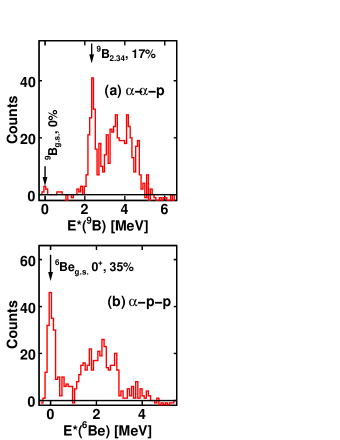
Figure 30: (Color online) Background-subtracted excitation-energy distributions for (a) ⁹B and (b) ⁶Be fragments produced in the decay of the 9.69-MeV level of ¹⁰C determined from p+2$\alpha$ and 2p+$\alpha$ triplets.

The distribution of $E_{pp}$, the relative kinetic energy between the two protons, is plotted in Fig. 31. This distribution shows a strong enhancement at small relative energies ($E_{pp}<$1.0 MeV), the diproton region, but also displays a tail to significantly higher values. Figures 32(a) and 32(b) show the distributions of ⁸Be and ⁵Li excitation energy determined from the detected $\alpha$-$\alpha$ pairs and all 4 combinations of p-$\alpha$ pairs. The total distributions (circular data points) have strong overlaps with the wide 3.03-MeV ⁸Be and the ⁵Li ground-state resonances, respectively. The distributions are rather insensitive to whether the events are associated with the diproton peak in Fig. 31 or associated with the higher-energy tail. To illustrate this, the squared data points in Fig. 32(a) and 32(b) show the distributions gated on the diproton peak ($E_{pp}<$1.0 MeV). Within the statistical uncertainties, they are the same shape as the ungated distributions.

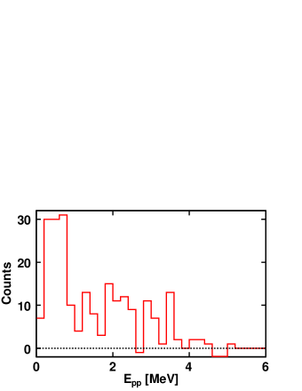
Figure 31: (Color online) Distribution of relative kinetic energy between the two protons for the 9.69-MeV level in ¹⁰C.

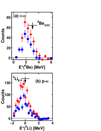
Figure 32: (Color online) Background-subtracted excitation-energy distributions for (a) ⁸Be and (b) ⁵Li fragments produced in the decay of the 9.69-MeV level of ¹⁰C determined from $\alpha$-$\alpha$ and p-$\alpha$ pairs. For the latter case, the distribution contains all four possible p-$\alpha$ pairs associated with each detected 2p+2$\alpha$ event. The distributions indicated by the circular data points have no restriction on the p-p relative energy, while for the squared-shaped data points $E_{pp}<$ 1.0 MeV. The arrows with error bars show the mean energy and width of the indicated resonances.

The strong overlap with the ⁵Li_g.s. resonance may initially suggest that the ¹⁰C fragment decays via the ⁵Li_g.s.+⁵Li_g.s. channel. However in such a case, the excitation energy reconstructed from an $\alpha$ particle and a proton originating from different ⁵Li fragments should populate the ⁵Li excitation energies significantly higher than ⁵Li_g.s. resonance region. However, the experimental data indicated that all four $\alpha$-p pairs are consistent with the ⁵Li_g.s. resonance. The decay thus appears to be four-body in nature and cannot be described by a sequential process. A possible interpretation is that all four p-$\alpha$ pairs are simultaneously in ⁵Li_g.s. resonances and some fraction of the p-p pairs are tightly correlated in a ”diproton”. Possibly, the $\alpha$-$\alpha$ pair may also be in a 3.03-MeV ⁸Be resonance. On the other hand, the overlap with the ⁵Li_g.s. and other resonances may just be coincidental. If all of these associations with resonances are correct, it is not clear that a configuration exists which would satisfy all of the implied angular momentum couplings. To display the correlations graphically, we note that each p+2$\alpha$ triplet in each 2p+2$\alpha$ event defines a plane in velocity space. With the two protons, we define two such planes in each event. The distribution of $\Delta\phi_{pp}$, the angle between these two planes is plotted in Fig. 33(a). This distribution resembles the relative-proton-energy distribution in Fig. 31 with a diproton region and a high-energy tail, and in fact the quantities $E_{pp}$ and $\Delta\phi_{pp}$ are strongly correlated.

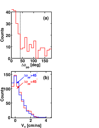
Figure 33: (Color online) Background-subtracted distributions associated with the decay of the 9.69-MeV state in ¹⁰C. (a) Distribution of the angle $\Delta\phi_{pp}$. This is the angle between the two planes in velocity space defined by the two $\alpha$ particles and each of the protons. (b) For the two indicated gates on $\Delta\phi_{pp}$, the distributions of the x component of the proton velocity (see text). For comparison purposes, the results for $\Delta\phi_{pp}>40^{\circ}$ have been normalized to the same number of counts as in the $\Delta\phi_{pp}<40^{\circ}$ distribution.

In order to help visualize the correlations between each proton and the two alpha particles, we have employed the procedure used to generate Fig. 12. For each p+2$\alpha$ triplet, the $\alpha$-particle and proton velocity vectors are projected into their decay plane. Subsequently they are rotated in this plane to align the locations of the $\alpha$ particles. The 2-dimensional velocity distributions are plotted in Fig. 34 for gates on the diproton region ($\Delta\phi_{pp}<40^{\circ}$) and the high-energy tail ($\Delta\phi_{pp}>40^{\circ}$).

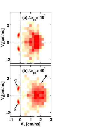
Figure 34: (Color online) Velocity distributions of $\alpha$ particles and protons produced in the decay of the 9.69-MeV state in ¹⁰C. For each 2$\alpha$+p triplet in each detected 2$\alpha$+2p event, the velocities have been projected onto the plane of the three fragments and rotated in this plane to align the locations of the $\alpha$ particles. The results are shown for (a) $\Delta\phi_{pp}<40^{\circ}$ and (b) $\Delta\phi_{pp}>40^{\circ}$ where the $\Delta\phi_{pp}$ is the angle between the two planes defined by the two protons.

Both distributions are quite similar and thus again there is little difference in the p-$\alpha$ correlations for the diproton and high-energy tail regions of the p-p relative energy. This is further illustrated in Fig. 33(b) where the projected $V_{x}$ distributions for these two regions are compared. Again we see very little difference in the results for the two gates. The average location of the two $\alpha$ particles and the proton form an isosceles triangle in their defining plane; i.e., the two p-$\alpha$ average relative velocities are identical and thus all p-$\alpha$ pairs can have the same reconstructed ⁵Li excitation energy.

V DISCUSSION AND CONCLUSIONS

This work highlights the wide range of many-particle decays of ground and excited states in light nuclei. It is not clear that there is a simple way of the predicting when the decays should be sequential or prompt. Certainly the presence of possible narrow intermediate states does not guarantee that the system will take advantage of them. For example the 9.69-MeV state in ¹⁰C has ⁶Be_g.s. and ⁹B_2.34 intermediate states with $\Gamma\sim$90 keV; yet 50% of the time it bypasses these and undergoes a 4-body decay. The 6.56 MeV state ¹⁰C also has competing prompt and sequential decay branches Charity09 . The nature of the decay is certainly related to the structure of the state and, in principle with suitable models, this information can be used to improve structure calculations. Presently there are only a few cases where prompt 3-body decay has been modeled in a sophisticated manner, as for example the quantum-mechanical cluster calculation Grigorenko09 , where comparisons to experimental correlations are useful. The prompt 4-body decay poses an even more difficult theoretical problem.

In this work we have studied many-particle exit channels associated with states formed following the interactions of an $E/A$=70 MeV ⁹C beam with a ⁹Be target. The decay products were detected in the HiRA array and the states were identified from the invariant mass of the detected fragments. Correlations between these fragments were used to deduce the nature of the decay and search for long-lived intermediate states associated with sequential decay processes. For such decays, angular correlations between the fragments provide information on the spin of the level.

The ground state of ⁸C disintegrates into four protons and an $\alpha$-particle. This decay was found to proceed through the ⁶Be_g.s. intermediate state, with two steps of 2-proton decay. The correlations between the protons in the first step exhibit a significant enhancement in a region of phase space where the two protons have small relative energy. The correlations in the second step were found to be consistent with ⁶Be_g.s. 2-proton decay obtained from an independent measurement using a ⁷Be beam.

Evidence suggests that the isobaric analog of this state in ⁸B, undergoes 2-proton decay to the isobaric analog of ⁶Be_g.s. in ⁶Li. This is the first case of two-proton decay between two isobaric analog states. The exact nature of the 2-proton decay awaits future measurements, but it may constitute a Goldansky-type decay with a single proton emission being energetically allowed but isospin forbidden.

A 9.69-MeV state of ¹⁰C was found, which $\sim$50% of the time, undergoes a prompt 4-body decay into the 2p+2$\alpha$ channel. There is a strong diproton-like correlation between the two protons, at the same time, all four possible p-$\alpha$ pairs have energies consistent with a ⁵Li_g.s. resonance. No sequential decay scenario is possible to produce 4 simultaneous ⁵Li_g.s. resonances.

Evidence for a prompt 3-body decay of the 8.15-MeV state of ⁸B was found. On the other hand, a number of states with three-body exit channels were observed that are well described as sequential decays through intermediate states. These include the isobaric pair, ⁸B_5.93 and ⁸Be_22.9, and the 11.7, 16.9 and 20.6 MeV states of ⁹B. The correlations in the decay of the 2.345-MeV state of ⁹B to the p + 2$\alpha$ channel were found to have strong sequential character associated with a ⁵Li intermediate, even though the lifetime of this intermediate state is very short and, at the very least, we would expect there to be very important final-state interactions.

Finally, new mass excesses and decay widths were obtained for the ground states of ⁷B and ⁸C.

- (1) V. I. Goldansky, Nuclear Physics 19, 482 (1960)
- (2) K. Miernik, W. Dominik, Z. Janas, M. Pfützner, L. Grigorenko, C. R. Bingham, H. Czyrkowski, M. Cwiok, I. G. Darby, R. Dkabrowski, T. Ginter, R. Grzywacz, M. Karny, A. Korgul, W. Kuśmierz, S. N. Liddick, M. Rajabali, K. Rykaczewski, and A. Stolz, Phys. Rev. Lett. 99, 192501 (2007)
- (3) B. Blank, A. Bey, G. Canchel, C. Dossat, A. Fleury, J. Giovinazzo, I. Matea, N. Adimi, F. De Oliveira, I. Stefan, G. Georgiev, S. Grévy, J. C. Thomas, C. Borcea, D. Cortina, M. Caamano, M. Stanoiu, F. Aksouh, B. A. Brown, F. C. Barker, and W. A. Richter, Phys. Rev. Lett. 94, 232501 (2005)
- (4) D. F. Geesaman, R. L. McGrath, P. M. S. Lesser, P. P. Urone, and B. VerWest, Phys. Rev. C 15, 1835 (1977)
- (5) L. V. Grigorenko, T. D. Wiser, K. Mercurio, R. J. Charity, R. Shane, L. G. Sobotka, J. M. Elson, A. H. Wuosmaa, A. Banu, M. McCleskey, L. Trache, R. E. Tribble, and M. V. Zhukov, Phys. Rev. C 80, 034602 (2009)
- (6) R. J. Charity, J. M. Elson, J. Manfredi, R. Shane, L. G. Sobotka, Z. Chajecki, D. Coupland, H. Iwasaki, M. Kilburn, J. Lee, W. G. Lynch, A. Sanetullaev, M. B. Tsang, J. Winkelbauer, M. Youngs, S. T. Marley, D. V. Shetty, A. H. Wuosmaa, T. K. Ghosh, and M. E. Howard, Phys. Rev. C 82, 041304 (2010)
- (7) M. S. Wallace, M. A. Famiano, M.-J. V. Goethem, A. M. Rogers, W. G. Lynch, J. Clifford, J. Lee, S. Labostov, M. Mocko, L. Morris, A. Moroni, B. E. Nett, D. J. Oostdyk, R. Krishnasamy, M. B. Tsang, R. D. de Souza, S. Hudan, L. G. Sobotka, R. J. Charity, J. Elson, and G. L. Engel, Nucl. Instrum. Methods A 583, 302 (2007)
- (8) G. L. Engel, M. Sadasivam, M. Nethi, J. M. Elson, L. G. Sobotka, and R. J. Charity, Nucl. Instrum. Methods A 573, 418 (2007)
- (9) R. J. Charity, S. A. Komarov, L. G. Sobotka, J. Clifford, D. Bazin, A. Gade, J. Lee, S. M. Lukyanov, W. G. Lynch, M. Mocko, S. P. Lobastov, A. M. Rogers, A. Sanetullaev, M. B. Tsang, M. S. Wallace, S. Hudan, C. Metelko, M. A. Famiano, A. H. Wuosmaa, and M. J. van Goethem, Phys. Rev. C 76, 064313 (2007)
- (10) J. F. Ziegler, J. P. Biersack, and U. Littmark, The Stopping and Range of Ions in Solids (Pergamon Press, New York, 1985) the code SRIM can be found at www.srim.org.
- (11) R. Anne, J. Herault, R. Bimbot, H. Gauvin, C. Bastin, and F. Hubert, Nucl. Instrum. Methods B 34, 295 (1988)
- (12) R. J. Charity, S. A. Komarov, L. G. Sobotka, J. Clifford, D. Bazin, A. Gade, J. Lee, S. M. Lukyanov, W. G. Lynch, M. Mocko, S. P. Lobastov, A. M. Rogers, A. Sanetullaev, M. B. Tsang, M. S. Wallace, R. G. T. Zegers, S. Hudan, C. Metelko, M. A. Famiano, A. H. Wuosmaa, and M. J. van Goethem, Phys. Rev. C 78, 054307 (2008)
- (13) A. M. Lane and R. G. Thomas, Rev. Mod. Phys. 30, 257 (1958)
- (14) F. C. Barker, Phys. Rev. C 59, 535 (1999)
- (15) L. C. Biedenharn and M. E. Rose, Rev. Mod. Phys. 25, 729 (1953)
- (16) H. Frauenfelder, Annu. Rev. Nucl. Sci. 2, 129 (1953)
- (17) Evaluated Nuclear Structure Data File (ENSDF), http://www.nndc.bnl.gov/ensdf/
- (18) G. Audi, A. H. Wapstra, and C. Thibault, Nucl. Phys. A729, 337 (2003)
- (19) R. G. H. Robertson, S. Martin, W. R. Falk, D. Ingham, and A. Djaloeis, Phys. Rev. Lett. 32, 1207 (1974)
- (20) R. G. H. Robertson, W. Benenson, E. Kashy, and D. Mueller, Phys. Rev. C 13, 1018 (1976)
- (21) R. E. Tribble, R. A. Kenefick, and R. L. Spross, Phys. Rev. C 13, 50 (1976)
- (22) O. V. Bochkarev, L. . V. Chulkov, A. A. Korsheninnikov, E. A. Kuz’min, I. G. Mukha, and G. B. Yankov, Nucl. Phys. A505, 215 (1989)
- (23) R. J. Charity, T. D. Wiser, K. Mercurio, R. Shane, L. G. Sobotka, A. H. Wuosmaa, A. Banu, L. Trache, and R. E. Tribble, Phys. Rev. C 80, 024306 (2009)
- (24) S. Cohen and D. Kurath, Nuclear Physics 73, 1 (1965)
- (25) S. Cohen and D. Kurath, Nuclear Physics A 101, 1 (1967), ISSN 0375-9474
- (26) B. A. Brown and F. C. Barker, Phys. Rev. C 67, 041304 (2003)
- (27) F. C. Barker, Phys. Rev. C 66, 047603 (Oct 2002)
- (28) F. C. Barker, Phys. Rev. C 67, 049902(E) (2003)
- (29) R. L. McGrath, J. Cerny, and E. Norbeck, Phys. Rev. Lett. 19, 1442 (1967)
- (30) L. Grigorenko, R. Johnson, I. Mukha, I. Thompson, and M. Zhukov, The European Physical Journal A - Hadrons and Nuclei 15, 125 (2002)
- (31) R. G. H. Robertson, W. S. Chien, and D. R. Goosman, Phys. Rev. Lett. 34, 33 (Jan 1975)
- (32) C. L. Woods, F. C. Barker, W. N. Catford, L. K. Fifield, and N. A. Orr, Aust. J. Phys. 41, 525 (1988)
- (33) F. C. Barker, Phys. Rev. C 68, 054602 (2003)
- (34) N. Chakraborty, B. D. Fields, and K. A. Olive(2010), arXiv:nucl-th/1011.0722v1
- (35) S. Dixit, W. Bertozzi, T. N. Buti, J. M. Finn, F. W. Hersman, C. E. Hyde-Wright, M. V. Hynes, M. A. Kovash, B. E. Norum, J. J. Kelly, A. D. Bacher, G. T. Emery, C. C. Foster, W. P. Jones, D. W. Miller, B. L. Berman, and D. J. Millener, Phys. Rev. C 43, 1758 (1991)
- (36) N. Curtis, N. L. Achouri, N. I. Ashwood, H. G. Bohlen, W. N. Catford, N. M. Clarke, M. Freer, P. J. Haigh, B. Laurent, N. A. Orr, N. P. Patterson, N. Soić, J. S. Thomas, and V. Ziman, Phys. Rev. C 77, 021301 (2008)
- (37) N. Curtis, N. L. Achouri, N. I. Ashwood, H. G. Bohlen, W. N. Catford, N. M. Clarke, M. Freer, P. J. Haigh, B. Laurent, N. A. Orr, N. P. Patterson, N. Soić, J. S. Thomas, and V. Ziman, Phys. Rev. C 82, 029907(E) (2010)