Wave packet dynamics and valley filter in strained graphene

Abstract

The time evolution of a wavepacket in strained graphene is studied within the tight-binding model and continuum model. The effect of an external magnetic field, as well as a strain-induced pseudo-magnetic field, on the wave packet trajectories and zitterbewegung are analyzed. Combining the effects of strain with those of an external magnetic field produces an effective magnetic field which is large in one of the Dirac cones, but can be practically zero in the other. We construct an efficient valley filter, where for a propagating incoming wave packet consisting of momenta around the $K$ and $K^{\prime}$ Dirac points, the outgoing wave packet exhibits momenta in only one of these Dirac points, while the components of the packet that belong to the other Dirac point are reflected due to the Lorentz force. We also found that the zitterbewegung is permanent in time in the presence of either external or strain-induced magnetic fields, but when both the external and strain-induced magnetic fields are present, the zitterbewegung is transient in one of the Dirac cones, whereas in the other cone the wave packet exhibits permanent spatial oscillations.

I Introduction

Since its first synthesis in 2004, Novoselov graphene has been attracting much interest due to its unique electronic properties arising from its singular energy spectrum, where in the vicinity of the points labelled as $K$ and $K^{\prime}$ in reciprocal space, the charge carriers behave as massless quasi-particles and exhibit an almost linear dispersion. CastroNeto These quasi-particles obey the Dirac-Weyl equations and therefore should be subject to quasi-relativistic effects, such as zitterbewegung, i.e., a trembling motion caused by interference between positive and negative energy states. Thaller ; Zawadzki1 ; David The phenomenon of zitterbewegung was predicted in 1930 by Schrödinger Schrodinger and has been subject of renewed interest over the past years. Previous theoretical works have suggested few ways of experimentally observing zitterbewegung, e. g. in narrow-gap semiconductors Zawadzki , in III-V zinc-blende semiconductor quantum wells with spin-orbit coupling Schliemann and, more recently, in monolayer Rusin1 and bilayer Wang graphene. An experimental simulation of the zitterbewegung of free relativistic electrons in vacuum was performed by Gerritsma et al. Gerritsma by using trapped ions.

Strain engineering in graphene has recently become a widely studied topic. PereiraECastroNeto1 ; Choi ; Pellegrino ; Treidel ; Fujita ; Chang The elastic properties of graphene nanoribbons were theoretically investigated by Cadelano et al.Cadelano , which studied the in-plane stretching and out of plane bending deformations by combining continuum elasticity theory and tight-binding atomistic simulations. Later, Cocco et al.Cocco and Lu and Guo Lu showed that a combination of shear and uniaxial strain at moderate absolute deformations can be used to open a gap in the graphene energy spectrum. It has been shown recently that specific forms of strain produce a pseudo-magnetic field in graphene, which does not break the time reversal symmetry and which points in opposite directions for electrons moving around the $K$ and $K^{\prime}$ points. Vozmediano The strain-induced magnetic field is expected to produce Landau levels and, consequently, the quantum Hall effect, even in the absence of an external magnetic field. Guinea ; Low Guinea et al., Guinea2 showed theoretically that an in-plane bending of the graphene sheet leads to an almost uniform field. Landau levels as a consequence of strain-induced pseudo-magnetic fields greater than 300 Tesla were recently observed with scanning tunnelling microscopy (STM) in nanometer size nanobubbles. Levy

Although previous works have studied wave packet propagation for the Dirac-Weyl Hamiltonian of graphene in the absence of external fields and potentials, Maksimova or in the presence of uniformly applied external magnetic fields Rusin1 ; Rusin2 ; Romera ; Krueckl , there is still a lack of theoretical works on the wave packet propagation through potential and (pseudo) magnetic field step barriers. Moreover, the time evolution of a wave packet in graphene within the tight-binding (TB) model, where the intra-valley scattering to higher energy states and inter-valley scattering due to defects appear naturally, is still hardly found in the literature. It is also interesting to see whether the results from Dirac and TB approaches for graphene differ or are similar.

In this paper, we investigate the time-evolution of wavepackets in graphene within the TB model, based on the split-operator technique for the expansion of the time-evolution operator. We trace a parallel between the results from the TB model and those obtained from the Dirac approximation for particles with momentum close to one of the Dirac cones of the Brillouin zone of graphene. The proposed method is then applied to the study of the dynamics of Gaussian wave packets in graphene under external magnetic fields. The effects of the pseudo-magnetic field induced by bending the graphene sheet into an arc of circle are analyzed as well. Our results show that for an appropriate choice of strain and external magnetic field strength, the system exhibits a strong effective magnetic field for particles in one of the Dirac cones, whereas in the other cone the external and pseudo-magnetic fields cancel each other and the effective magnetic field is practically zero. We show that this effect is manifested as a transient (permanent) zitterbewegung for electrons in the cone where the effective magnetic field is zero (non-zero), which can be verified experimentally by detecting the electric field radiation emitted by the trembling wave packet. Rusin2 Moreover, our results show that with such a choice of external and strain-induced magnetic fields, one can construct an efficient valley-filter, which can be useful for future valley-tronic devices. Rycerz

II Time evolution operator

By solving the time-dependent Schrödinger equation, one obtains that the propagated wavefunction after a time step $\Delta t$ can be calculated by applying the time-evolution operator on the wave packet at any instant $t$

$$\Psi(\vec{r},t+\Delta t)=e^{-\frac{i}{\hbar}H\Delta t}\Psi(\vec{r},t),$$ (1)

where we assumed that the Hamiltonian $H$ is time-independent. Different techniques have been suggested for the expansion of the exponential in Eq. (1), e.g. the Chebyschev polynomials method Fehske and the second order differencing scheme Mahapatra ; Kosloff . The numerical method that we use for the application of the time evolution operator in this work, namely, the split-operator method, Chaves is the subject of this section, where we will show how this technique can be adapted for the study of the wave packet dynamics in graphene within the tight-binding and Dirac approximations.

II.1 Tight-Binding model

Graphene consists of a layer of carbon atoms forming a honeycomb lattice, which can be described by the Hamiltonian

$$H_{TB}=\sum_{i}\epsilon_{i}c^{\dagger}_{i}c_{i}+\sum_{<i,j>}\left[\tau_{ij}c^{\dagger}_{i}c_{j}+\tau^{*}_{ij}c_{i}c_{j}^{\dagger}\right],$$ (2)

where $c_{i}$($c_{i}^{\dagger}$) annihilates (creates) an electron at the site $i$, with on-site energy $\epsilon_{i}$, and the sum is taken only between nearest neighbor sites $i$ and $j$, with hopping energy $\tau_{ij}$. The effect of an external magnetic field can be calculated by including a phase in the hopping parameters according to the Peierls substitution $\tau_{ij}\rightarrow\tau_{ij}\exp\left[i\frac{e}{\hbar}\int_{j}^{i}\vec{A}\cdot d\vec{l}\right]$, where $\vec{A}$ is the vector potential describing the magnetic field. Bahamon ; Governale In a strained graphene sheet, the distance between two adjacent sites $i$ and $j$ is changed by $\Delta a_{ij}=a_{ij}-a_{0}$, where $a_{0}$ is the lattice parameter of unstrained graphene and $a_{ij}$ is the distance between the sites after the stress. The change in the inter-sites distance affects the hopping energy between the sites, which becomes Vozmediano $\tau_{ij}\rightarrow\tau_{ij}\left(1+2\Delta a_{ij}/a_{0}\right)$. A similar expression can be obtained by expanding Eq. (13) of Ref. PereiraECastroNeto, in Taylor series and neglecting higher order terms in $\Delta a_{ij}$, i.e., considering small lattice deformations. The strain-induced change in the hopping energies leads to an effective pseudo-magnetic field, which points to opposite directions in the valley $K$ and $K^{\prime}$. Guinea Notice that the pseudo-magnetic field in our model is not introduced artificially by considering an additional vector potential in the Peierls phase, but it rather appears naturally after the changes in the inter-site distances due to the strain.

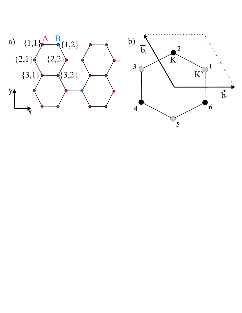
Figure 1: (Color online) (a) Sketch of the honeycomb lattice of graphene, made out of two superimposed triangular lattices $A$ and $B$. The atoms are labelled as $\{n,m\}$ according to their line and column numbers $n$ and $m$, respectively. (b) Reciprocal lattice of graphene, with $K$ (black) and $K^{\prime}$ (gray) Dirac points, where the area defined by the reciprocal vectors $\vec{b}_{1}=(-2\pi/3a_{0},\sqrt{3})$ and $\vec{b}_{2}=(4\pi/3a_{0},0)$ represents the first Brillouin zone. The numbers close to each Dirac point are explained in the text.

Let us label the sites $i$ of the graphene lattice according to their line and column numbers $n$ and $m$, respectively, as shown in Fig. 1(a). The basis vector state $|n,m\rangle$ represents an electron confined on the site of line $n$ and column $m$. In a lattice consisting only of non-interacting sites, each $|n,m\rangle$ is an eigenstate of $H_{TB}$ with energy $\epsilon_{n,m}$, i.e. $H_{TB}|n,m\rangle=\epsilon_{n,m}|n,m\rangle$. Limiting ourselves to nearest neighbors interactions, we find

$$H_{TB}|n,m\rangle=\epsilon_{nm}|n,m\rangle+T_{m+1}|n,m+1\rangle\quad\quad\quad$$

$$+T_{m-1}|n,m-1\rangle+T_{n+1}|n+1,m\rangle+T_{n-1}|n-1,m\rangle,$$ (3)

where $T_{n\pm 1}$ and $T_{m\pm 1}$ are equivalent to the hopping energies $\tau_{ij}$ between the site $i=\{n,m\}$ and the adjacent sites $j=\{n\pm 1,m\}$ and $j=\{n,m\pm 1\}$, respectively. Eq. (II.1) can be rewritten as

$$H_{TB}|n,m\rangle=H_{n}|n,m\rangle+H_{m}|n,m\rangle,$$ (4)

where the operators $H_{n}$ and $H_{m}$ are defined as

$$H_{n}|n,m\rangle=T_{m+1}|n,m+1\rangle+T_{m-1}|n,m-1\rangle+\frac{\epsilon_{nm}}{2}$$ (5a)

and

$$H_{m}|n,m\rangle=T_{n+1}|n+1,m\rangle+T_{n-1}|n-1,m\rangle+\frac{\epsilon_{nm}}{2}.$$ (5b)

The wavefunction at any instant $t$ is then written as a linear combination of the basis vector states $\Psi^{t}_{n,m}=\sum_{n,m}b^{t}_{n,m}|n,m\rangle$. The advantage of following the procedure described by Eqs. (II.1-5) lies in the fact that the operators $H_{n}$ and $H_{m}$ in Eq. (5) can be represented by tri-diagonal matrices, which are easier to handle than the matrix representing the full Hamiltonian, Eq. (II.1).

The split-operator technique can now be applied to the Hamiltonian Eq. (4), so that the time evolution operator is approximated by

$$e^{-\frac{i}{\hbar}H_{TB}\Delta t}=e^{-\frac{i}{2\hbar}H_{m}\Delta t}e^{-\frac{i}{\hbar}H_{n}\Delta t}e^{-\frac{i}{2\hbar}H_{m}\Delta t}+O(\Delta t^{3}),$$ (6)

where the error comes from the non-commutativity between the operators $H_{n}$ and $H_{m}$. We drop the $O(\Delta t^{3})$ terms by considering a small time step $\Delta t=0.1$ fs. The propagated wavefunction is then obtained from Eq. (1), which in this case reads

$$\Psi^{t+\Delta t}_{n,m}=e^{-\frac{i}{2\hbar}H_{m}\Delta t}e^{-\frac{i}{\hbar}H_{n}\Delta t}e^{-\frac{i}{2\hbar}H_{m}\Delta t}\Psi^{t}_{n,m}.$$ (7)

This equation is solved in three steps:

$$\eta_{n,m}=e^{-\frac{i}{2\hbar}H_{m}\Delta t}\Psi^{t}_{n,m},$$ (8a)

$$\xi_{n,m}=e^{-\frac{i}{\hbar}H_{n}\Delta t}\eta_{n,m},$$ (8b)

$$\Psi^{t+\Delta t}_{n,m}=e^{-\frac{i}{2\hbar}H_{m}\Delta t}\xi_{n,m}.$$ (8c)

Using the Cayley form for the exponentials, Watanabe we can rewrite Eq. (8a) as

$$\eta_{n,m}=e^{-\frac{i}{2\hbar}H_{m}\Delta t}\Psi^{t}_{n,m}=\frac{1-\frac{i\Delta t}{4\hbar}H_{m}}{1+\frac{i\Delta t}{4\hbar}H_{m}}\Psi^{t}_{n,m}+O(\Delta t^{2}),$$ (9)

which leads to

$$\left(1+\frac{i\Delta t}{4\hbar}H_{m}\right)\eta_{n,m}\approx\left(1-\frac{i\Delta t}{4\hbar}H_{m}\right)\Psi^{t}_{n,m}.$$ (10)

As the wavefunction $\Psi^{t}_{n,m}$ is already known, the matrix equation in Eq. (10) can be straightforwardly solved to obtain $\eta_{n,m}$. We repeat this procedure for the other two exponentials in Eqs. (8b) and (8c), and eventually obtain $\Psi^{t+\Delta t}_{n,m}$.

In fact, the form in Eq. (10) can also be applied to the full Hamiltonian $H_{TB}$, i.e. without splitting the $H_{m}$ and $H_{n}$ terms. However, this would lead to matrix equations involving penta-diagonal matrices, which are harder to handle than the tri-diagonal matrices in Eq. (10). As the error produced by the splitting in Eq. (7) is smaller than the error produced by the (necessary) expansion of the exponential given by Eq. (10), it is worthy to split these terms in order to simplify the numerical calculations.

II.2 Dirac-Weyl equation

From the TB Hamiltonian Eq. (2), considering an infinite graphene sheet in the absence of external potential and magnetic fields, one obtains the energy bandstructure of graphene as

$$E\left(\vec{k}\right)=\pm\tau\sqrt{3+f\left(\vec{k}\right)}$$

$$f\left(\vec{k}\right)=2\cos\left(\sqrt{3}k_{y}a_{0}\right)+4\cos\left(\frac{\sqrt{3}}{2}k_{y}a_{0}\right)\cos\left(\frac{3}{2}k_{x}a_{0}\right),$$ (11)

which is gapless in six points of the reciprocal space where $E=0$, from which only two are inequivalent, labelled as $K$ and $K^{\prime}$, as shown in Fig. 1(b). CastroNeto ; PereiraReview In the vicinity of each of these points, the dependence of the energy spectrum on the wave vector $\vec{k}$ is almost linear and the electron can be described as a massless fermion by the Dirac Hamiltonian

$$H_{D}=\left[v_{F}\vec{\sigma}\cdot(\vec{\textsf{p}}+e\vec{A})+V(\textsf{x},\textsf{y})\textbf{I}\right]e^{-i\phi},$$ (12)

where $v_{F}=3\tau a_{0}/2\hbar$ is the Fermi velocity, $\vec{A}$ is the electromagnetic vector potential, $V(x,y)$ is an external potential, I is the identity matrix, $\vec{\sigma}$ is the Pauli vector and the wavefunctions are pseudo-spinors $\Psi=[\Psi_{A},\Psi_{B}]^{T}$, with $\Psi_{A(B)}$ as the probability of finding the electron in the sub-lattice $A(B)$ that composes the honeycomb lattice of graphene. CastroNeto The angle $\phi$ is different for electrons around the $K$ and $K^{\prime}$ Dirac cones. In the vicinity of the $k$-th Dirac point (see labels for each Dirac point in Fig. 1(b)), one obtains $\phi=-\pi/6+k\pi/3$, with $k=1-6$. From here onwards, we will refer to the coordinates in the Dirac (TB) model as x ($x$) and y ($y$).

The exponential term in Eq. (12) is usually dropped, because it can be considered as a phase in the state vectors in the Dirac model. However, this term has an important meaning when comparing with the TB model: this exponential can be identified as a rotation operator with angle $\phi$. Notice that an infinite graphene hexagonal lattice has C_6v symmetry, i.e. it is symmetric only for rotation angles $k\pi/3$ ($k$ - integer). As a consequence, the Dirac Hamiltonian Eq. (12) without the exponential term is not symmetric in the momenta $\hat{p}_{x}$ and $\hat{p}_{y}$, as already pointed out previously. Rusin1 So, what would be the meaning of the direction-dependent observables in the Dirac description of graphene, when they are not symmetric under rotation, exhibiting a privileged direction? Defining $y$ ($x$) as the zigzag (armchair) direction, as in Fig. 1(a), the results obtained by the Dirac approximation for the x and y components of any observable are compared to the armchair and zigzag directions, respectively, after performing a rotation $\phi$ in the coordinates of the Dirac model. From the possible values of $\phi$, one deduces straightforwardly that at any Dirac cone, the coordinate x (y) of the Dirac model is always related to one of the zigzag (armchair) directions of the real graphene lattice. On the other hand, for finite rectangular samples the different angles $\phi$ represent two distinguishable situations, since the rectangle does not share the C_6v symmetry of the infinite graphene lattice: the x direction in the Dirac model for the odd (even) cones in Fig. 1(b) represents a diagonal (vertical) direction in the rectangle. The comparison between the TB model for a rectangular graphene flake and the Dirac approximation will be discussed in details further, in the following section.

In a recent work, Maksimova et al. Maksimova presented an analytical study of the time evolution of a Gaussian wave packet in graphene in the absence of external potentials and/or magnetic fields within the continuum model, i. e. using the Dirac-Weyl Hamiltonian for electrons in the vicinity of the Dirac point $K$. In this paper, we will use an alternative and more general way of calculating the dynamics of a wavepacket in such a system, PereiraReview based on the split-operator technique, which can be applied for systems under arbitrary external potentials and magnetic fields.

The Dirac-Weyl Hamiltonian $H_{D}$ in Eq. (12) can be separated as $H_{D}=H_{k}+H_{r}$, where $H_{k}=\hbar v_{F}\vec{\sigma}\cdot\vec{\textsf{k}}$ keeps only the terms which depend on the wave vector $\vec{\textsf{k}}$, whereas $H_{r}=v_{F}e\vec{\sigma}\cdot\vec{A}+V\textbf{I}$ depends only on the real space coordinates x and y. Following the split-operator method, the time evolution operator for the Hamiltonian $H_{D}$ can be approximated as

$$\exp\left[-\frac{i\Delta t}{\hbar}\left(H_{k}+H_{r}\right)\right]\approx\quad\quad\quad\quad$$

$$\exp\left[-\frac{i\Delta t}{2\hbar}H_{r}\right]\exp\left[-\frac{i\Delta t}{\hbar}H_{k}\right]\exp\left[-\frac{i\Delta t}{2\hbar}H_{r}\right]$$ (13)

with an error of the order of $O(\Delta t^{3})$, due to the non-commutativity of the operators involved. We invoke a well-known property of the Pauli vectors

$$\exp\left(-i\vec{S}\cdot\vec{\sigma}\right)=\cos(S)\textbf{I}-i\frac{\sin(S)}{S}\left(\vec{S}\cdot\vec{\sigma}\right)$$ (14)

for any vector $\vec{S}$, where $S=|\vec{S}|$, and rewrite the exponentials in real and reciprocal space, respectively, in matrix form

$$\textbf{M}_{r}=\left[\cos\left(\textsf{A}\right)\textbf{I}-i\frac{\sin\left(\textsf{A}\right)}{\textsf{A}}\left(\begin{array}[]{cc}0&\textsf{A}_{\textsf{x}}-i\textsf{A}_{\textsf{y}}\\ \textsf{A}_{\textsf{x}}+i\textsf{A}_{\textsf{y}}&0\\ \end{array}\right)\right]e^{-\frac{i\Delta t}{2\hbar}V}$$ (15a)

$$\textbf{M}_{k}=\cos(\kappa)\textbf{I}-i\frac{\sin(\kappa)}{\kappa}\left(\begin{array}[]{cc}0&\kappa_{x}-i\kappa_{y}\\ \kappa_{x}+i\kappa_{y}&0\\ \end{array}\right),$$ (15b)

where $\textsf{A}=|\vec{\textsf{A}}|=\Delta tv_{F}e|\vec{A}|\big{/}2\hbar$, $\vec{\kappa}=\Delta tv_{F}\vec{\textsf{k}}$ and $\kappa=|\vec{\kappa}|=\Delta tv_{F}\sqrt{\textsf{k}_{\textsf{x}}^{2}+\textsf{k}_{\textsf{y}}^{2}}$, so that the time evolution of a wave packet $\Psi_{D}(x,y)=[\phi_{A},\phi_{B}]^{T}\Psi(x,y)$ can be calculated as a series of matrix multiplications

$$\Psi(\vec{\textsf{r}},t+\Delta t)=\textbf{M}_{r}\cdot\textbf{M}_{k}\cdot\textbf{M}_{r}\Psi(\vec{\textsf{r}},t)+O(\Delta t^{3}).$$ (16)

The matrix multiplication by $\textbf{M}_{k}$ is made in reciprocal space by taking the Fourier transform of the functions. In the absence of magnetic fields and external potentials, one has M_r = I and

$$\Psi(\vec{\textsf{r}},t+\Delta t)=\textbf{M}_{k}\Psi(\vec{\textsf{r}},t),$$ (17)

where the matrix multiplication in reciprocal space gives the exact result for the time evolution of the wave packet, since there is no error induced by non-commutativity of operators or matrices in this case. This shows that the split-operator method provides a way to study the dynamics of wavepackets in graphene within the continuum model where, in the presence of magnetic fields and/or external potentials, one can control the accuracy of the results by making $\Delta t$ smaller, while in their absence, the problem is solved exactly by a simple matrix multiplication for any value of $\Delta t$.

III Results and discussion

We shall now discuss the results obtained for a graphene lattice with 2000$\times$3601 atoms, with armchair (zigzag) edges in the $x$($y$)-direction. The nearest neighbors hopping parameter and the lattice constant of graphene are taken as $\tau=-2.7$ eV and $a_{0}=1.42$ Å , respectively.

As initial wave packet, we consider a Gaussian centered at $\vec{r_{0}}=(x_{0},y_{0})$ in real space and $\vec{q}=(q_{x}^{0},q_{y}^{0})$ in reciprocal space:

$$\Psi_{q}(\vec{r})=N\left(\begin{array}[]{c}c_{1}\\ c_{2}\\ \end{array}\right)\exp\left[-\frac{(x-x_{0})^{2}+(y-y_{0})^{2}}{2d^{2}}+i\vec{q}\cdot\vec{r}\right],$$ (18)

where $N$ is the normalization factor. Notice that we have included a pseudo-spinor $[c_{1},c_{2}]^{T}$ in the initial wave packet, where $c_{1(2)}$ is the probability of finding the electron in the triangular sub-lattice $A(B)$ that composes the graphene hexagonal lattice. One can also rewrite the pseudo-spinor as $[1,e^{i\theta}]^{T}$, where the pseudo-spin polarization angle $\theta$ is shown explicitly. The pseudo-spin is a concept normally attributed to the Dirac description of graphene. Indeed, the pseudo-spin of a wavefunction in the Dirac model is related to the expectation values of the Pauli matrices $\langle\sigma_{i}\rangle$, which can involve integrals of the product between wavefunctions for sub-lattices $A$ and $B$. Such a definition fails for the TB wavefunctions, since in this case they are defined in different points of the lattice, so that any integral that mixes functions of both sub-lattices gives zero. Even so, the study of the pseudo-spin related to the initial discrete wave packet helps to understand the wave packet dynamics obtained from the TB model, as we will see further in this section.

III.1 Initial pseudo-spin polarization and zitterbewegung revisited

In this subsection, we will use the TB model to review some of the main properties of the wave packet dynamics in graphene. Within the TB model, we consider the initial wave packet as a discrete form of the Gaussian distribution in Eq. (18) for the graphene hexagonal lattice, where we multiply the Gaussian function by $c_{1(2)}$ in the sites belonging to the triangular sub-lattice $A(B)$. From Eq. (II.2), it is clear that in momentum space, the region of interest is the vicinity of the Dirac points $K$ and $K^{\prime}$, since the energy corresponding to wave vectors out of this region is very high.

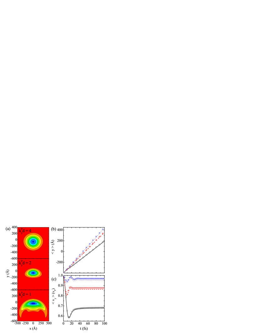
Figure 2: (Color online)(a) Contour plots of the squared modulus of the wavefunction after a time evolution of $t=40$ fs, for three different values of the dimensionless parameter $k_{y}^{0}d$. (b) Expectation value of the position and (c) velocity in $y$-direction as a function of time. The results obtained from the TB (Dirac) model are presented as curves (symbols), for $k_{y}^{0}d=1$ (solid, circles), 2 (dashed, triangles) and 4 (dotted, squares)

In the TB model for two-dimensional crystals, one usually considers the same Gaussian distribution for all the sites of the lattice. Nazareno This is equivalent as choosing $c_{1}=c_{2}=1$ in Eq. (18). Figure 2(a) shows the contour plots of the squared modulus of the propagated wavefunctions at $t=40$ fs for these values of $c_{i}$, considering an initial wave vector $\vec{q}=(0,k_{y}^{0})+K$, i.e. in the vicinity of the $K$ point labelled as 2 in Fig. 1(b). As shown in Ref. Maksimova, , the wave packet dynamics near the Dirac cones in graphene does not depend separately on the momentum $k_{y}^{0}$ or on the width $d$, but rather on the dimensionless quantity $k_{y}^{0}d$. This result was obtained from the Dirac model for graphene, i.e. considering that even high energies states exhibit linear dispersion. Within the TB model we expect that wave packets with the same $k_{y}^{0}d$ behave alike only if $k_{y}^{0}$ is not too far from the Dirac cone and if $d$ is not too small, so that the packet is well localized in energy space. Within these conditions, Fig. 2 shows the time evolution for different values of this dimensionless quantity: $k_{y}^{0}d=1$ and 2, with $d=100$ Å , and $k_{y}^{0}d=4$, with $d=200$ Å . We observe that the dispersion of the wave packet is stronger for smaller values of $k_{y}^{0}d$, where it becomes distorted into an arc-like shape. For larger $k_{y}^{0}d$, on the other hand, the wave packet keeps its circularly symmetric shape for longer times.

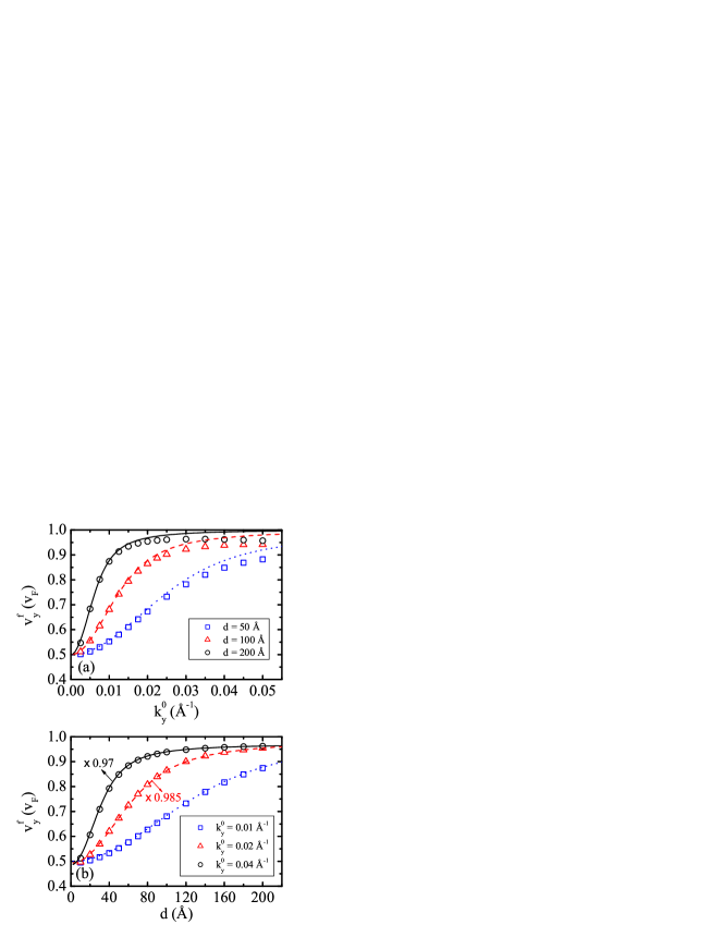
Figure 3: (Color online) Final velocities for the Gaussian wave packet in Eq. (18), with pseudo-spin $c_{1}=c_{2}=1$ and momentum $\vec{q}=(0,k_{y}^{0})+K$ as a function of (a) the momentum $k_{y}^{0}$, for widths $d=50$ Å , 100 Å  and 200 Å , and (b) the width $d$, for momenta $k_{y}^{0}=0.01$ Å ^-1, 0.02 Å ^-1 and 0.04 Å ^-1. The symbols (curves) are obtained from the TB (Dirac) model. In (b), the results from the Dirac model for $k_{y}^{0}=$ 0.02 Å ^-1 (dashed) and 0.04 Å ^-1 (solid) are multiplied by 0.985 and 0.97, respectively.

As explained in the previous subsection, in order to obtain the Dirac Hamiltonian Eq. (12), one must shift the origin of the wave vectors $\vec{k}$ to one of the six Dirac points shown in Fig. 1(b). Besides, one must also rotate the $x$ and $y$ axis by an angle $\phi$ which depends on the $K$ or $K^{\prime}$ point that is considered as the origin in momentum space. For the $K=(0,4\pi\big{/}3\sqrt{3}a_{0})$ point, labelled as 2 in Fig. 1(b), the Dirac Hamiltonian Eq. (12) is obtained by rotating the axis by 90^∘, with other words, by a transformation of the coordinates as $x\rightarrow-\textsf{y}$ and $y\rightarrow\textsf{x}$. The pseudo-spinor $c_{1}=c_{2}=1$ represents a wave packet polarized in x-direction, i.e. $\langle\sigma_{x}\rangle>0$ and $\langle\sigma_{z}\rangle=\langle\sigma_{y}\rangle=0$. From the Heisenberg picture, we obtain the velocity in the x-direction for the proposed wave packet as

$$\frac{d\textsf{x}}{dt}=\frac{1}{i\hbar}\left[\textsf{x},H_{D}\right]=v_{F}\sigma_{x}.$$ (19)

Performing the appropriate coordinate transformations, the velocity obtained from the TB model for the $y$-direction must be consistent with the prediction from the Dirac approximation, namely, $v_{y}=d\textsf{x}/dt=v_{F}\sigma_{x}$. This suggests that such a wave packet propagates towards the positive $y$-direction, but with non-constant velocity, since $\sigma_{x}$ does not commute with $H_{D}$. The expectation value of the $y$ position of the packet $\langle y\rangle$ is shown as a function of time by the curves in Fig. 2(b), for $k_{y}^{0}d=1$ (solid), 2 (dashed) and 4 (dotted), where the results obtained by the Dirac equation are shown as symbols for comparison. A different linear behavior is already observed for each wave packet at large time, implying that they have different velocities, which is kind of counter-intuitive, since low-energy electrons in graphene are expected to propagate always with the same Fermi velocity $v_{F}$. Figure 2(c) shows the velocity $v_{y}$, calculated by taking the derivative of the TB results for $\langle y\rangle$ with respect to time, which exhibits clear oscillations that are damped as time evolves, converging to a final value $v^{f}_{y}<v_{F}$ that depends on the initial wave packet’s width $d$ and wave vector $k_{y}^{0}$. The velocities obtained by the Dirac model are shown by symbols, where the same qualitative behavior is observed as obtained from the TB model, though for higher wave packet momentum and width, a small quantitative difference is observed, which is a consequence of the different energy-momentum dispersion.

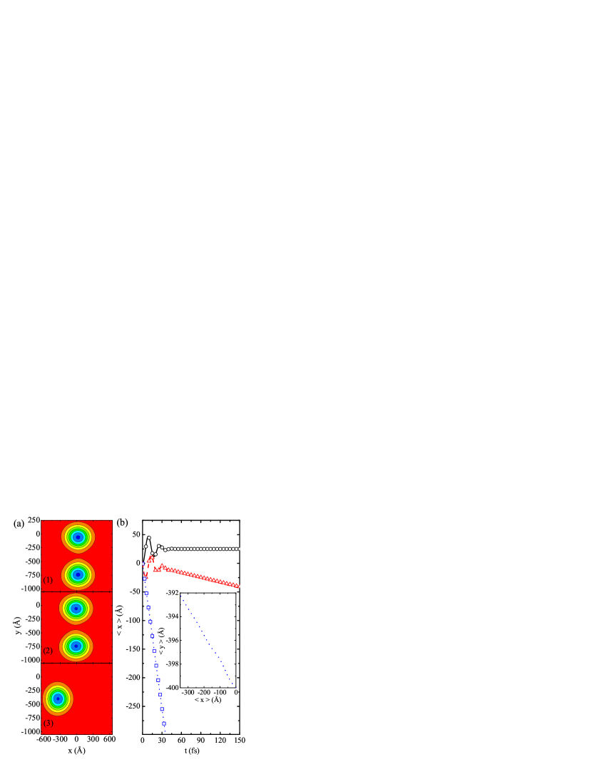
Figure 4: (Color online)(a) Contour plots of the squared modulus of the wavefunction after a time evolution of $t=40$ fs, for three initial configurations of pseudo-spin $[c_{1},c_{2}]^{T}$ and momentum $\vec{q}_{0}$: 1) $[1,0]^{T}$, $k_{x}^{0}=0$ and $k_{y}^{0}d=4$; 2) $[1,i]^{T}$, $k_{x}^{0}=0$ and $k_{y}^{0}d=4$; and 3) $[1,i]^{T}$, $k_{x}^{0}d=4$, $k_{y}^{0}=0$. (b) Expectation value of $x$ obtained by the TB model for the initial wavepackets 1 (solid), 2 (dashed) and 3 (dotted) as a function of time. The results obtained by the Dirac model, after the appropriate coordinates rotation (see text), are shown as circles, triangles and squares, respectively. The inset shows the trajectory of the wavepacket obtained from the TB model for the initial wavepacket 3.

The oscillatory behavior of the velocity is a manifestation of the zitterbewegung, i.e. a trembling motion of the wave packet due to the interference between positive and negative energy states that makes up the initial Gaussian wave packet. Rusin1 ; Thaller This effect is well-known for relativistic particles, which are described by the Dirac equation, and is also observed for electrons in graphene in the vicinity of the $K$ and $K^{\prime}$ points, since they can be described as massless quasi-particles by the Dirac equation as well. The velocity wiggles with shorter period and smaller amplitudes for larger values of $k_{y}^{0}d$. The convergence of the velocities demonstrates that the zitterbewegung is not a permanent, but a transient effect. Rusin1

Figure 3 shows the converged velocity $v^{f}_{y}$ as a function of (a) the momentum $k^{0}_{y}$ and (b) the width $d$ of the Gaussian wave packet. The TB results (symbols) are compared to those calculated from Eq. (31) in Ref. Maksimova, (curves), which was obtained analytically from the Dirac approximation in the $t\rightarrow\infty$ limit and is repeated here just for completeness:

$$\frac{v^{f}_{y}}{v_{F}}=1-\frac{1-e^{-(k^{0}_{y}d)^{2}}}{2(k^{0}_{y}d)^{2}}.$$ (20)

Within the Dirac model, one can observe that increasing $d$ or $k_{y}^{0}$ in Eq. (20), the final velocity increases monotonically and approaches $v_{F}$, which is reasonable, since a wider packet in real space leads to a narrower distribution in $k$-space, whereas a higher value of the wave vector makes the center of the packet lay far from $E=0$. In both cases, the interference with negative energy states is reduced and, consequently, zitterbewegung effects are less significant. However, since the analytical formula Eq. (20) does not take into account any effect such as the curvature of the energy bands for higher energy states or trigonal warping effects, this formula is not expected to give accurate results for larger $k^{0}_{y}$. Indeed, Fig. 3(a) shows that a very good agreement between TB and Dirac results can be observed only for small values of $k^{0}_{y}$, whereas for large $k^{0}_{y}$, the final velocities obtained from the TB model are lower than those obtained from the Dirac model and do not increase monotonically, but decreases slowly for very large $k^{0}_{y}$, as a consequence of the curvature of the energy bands. On the other hand, in Fig. 3(b) we observe that varying the wave packet width for a fixed momentum, good qualitative agreement with the Dirac model is obtained for almost any value of $d$. The curves for larger values of $k^{0}_{y}$ (solid and dashed) are just quantitatively different from those obtained by the TB model, and they are comparable to the TB results after multiplication by a factor 0.985 (0.970) for $k^{0}_{y}=0.02$ Å ^-1 (0.04 Å ^-1). Worse qualitative agreement between TB and Dirac results in this case is observed only for very small $d$, where the Gaussian width in energy space, given by $\Delta E=v_{F}\hbar d^{-1}$, incorporates higher energy values, leading to deviations in $v^{f}_{y}$ obtained from the TB model as compared to those from the Dirac model.

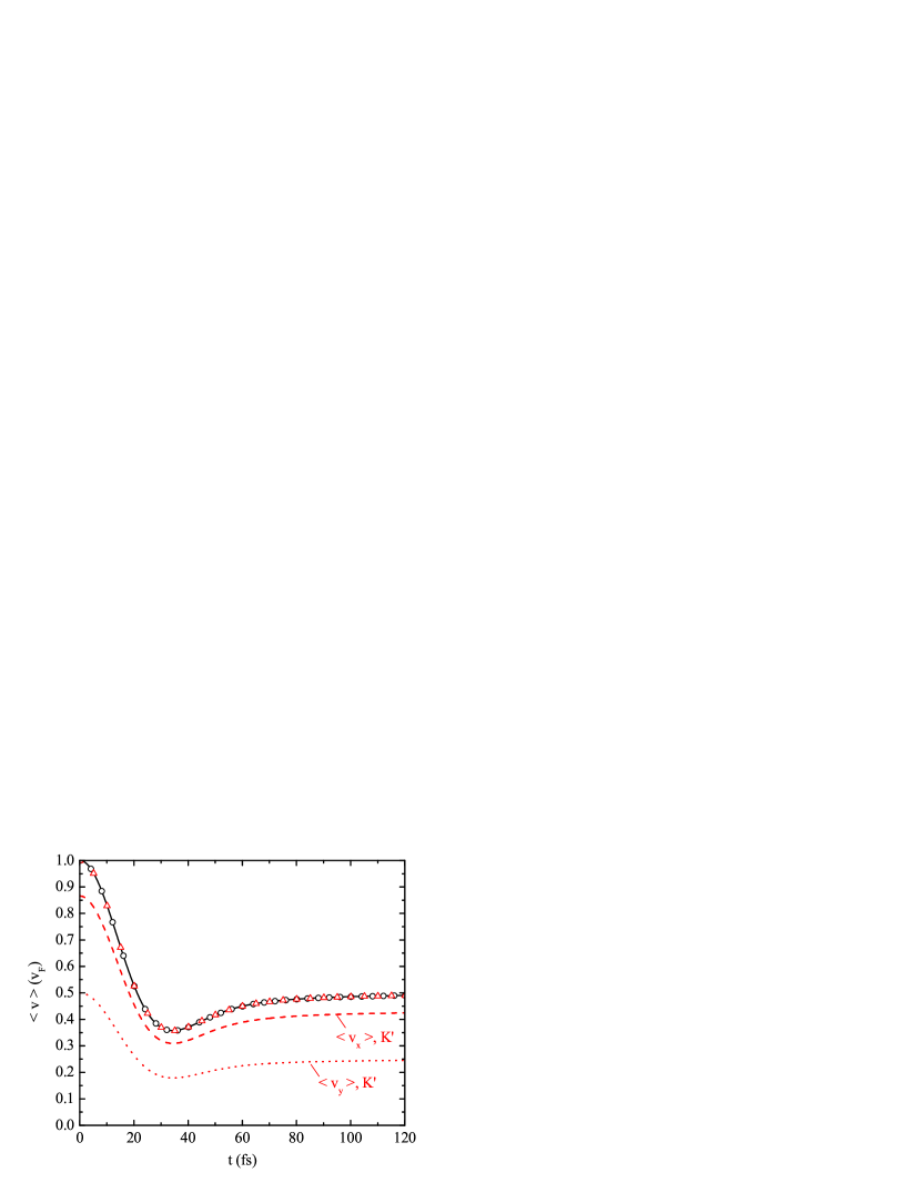
Figure 5: (Color online)(a) Expectation value of the velocity as a function of time, for wavepackets with $k_{y}^{0}=k_{x}^{0}=0$ and pseudo-spinor $[1,1]^{T}$ (solid) and $[1,i]^{T}$ (circles) at the Dirac point $K=(0,4\pi\big{/}3\sqrt{3}a_{0})$ (point 2 in Fig. 1(b)), and $[1,1]^{T}$ (triangles) at $K^{\prime}=(2\pi\big{/}3a_{0},2\pi\big{/}3\sqrt{3}a_{0})$ (point 1 in Fig. 1(b)). The $x$ and $y$ components of the velocity in the latter case are shown as dashed and dotted curves, respectively.

In Fig. 4(a) we show contour plots of the squared modulus of the wave function at $t=40$ fs for three different choices of wave vectors $\vec{q}=(k_{x}^{0},k_{y}^{0})+K$ and initial pseudo-spinors: 1) $[1,0]^{T}$, with $k_{x}^{0}=0$ and $k_{y}^{0}d=4$, 2) $[1,i]^{T}$, with $k_{x}^{0}=0$ and $k_{y}^{0}d=4$, and 3) $[1,i]^{T}$, with $k_{x}^{0}d=4$ and $k_{y}^{0}=0$. The curves (symbols) in Fig. 4(b) show the expectation value $\langle x\rangle$ for each case obtained by the TB (Dirac) model. In case 1 (solid, circles), the pseudo-spinor points in the $z$-direction, so that $\langle\sigma_{x}\rangle=\langle\sigma_{y}\rangle$ and, consequently, the velocity for both in-plane directions must be zero. Indeed, the wave packet splits into two equal parts that propagate in opposite $y$ directions, leading to $v_{y}=0$. In the $x$-direction, although there is still a small zitterbewegung, $\langle x\rangle$ rapidly converges to a constant, leading to $v_{x}=0$. In case 2 (dashed, triangles), the pseudo-spinor points in the y-direction, but the momentum of the wave packet in this direction is zero, so that the packet splits in the $y$-direction, since $v_{y}=v_{F}\sigma_{x}=0$, but drifts slowly in the $-x$ direction (or, equivalently, y). In case 3 (dotted, squares), both the pseudo-spin and the momentum are in the y-direction, so that the wave packet propagates in this direction without any splitting. This situation is comparable to the one in Fig. 2(a), since in both cases the pseudo-spin and momentum are in the same direction and, as a consequence, the wave packet propagates in this direction practically preserving its circular symmetry. However, in the case 3, the packet still presents a very weak oscillation in the $y$-direction, and also drifts very slowly in this direction, as one can see from the trajectory of the packet in the $x-y$ plane for this case, shown in the inset of Fig. 4(b). This oscillation and drift are related to the contributions of higher energy states in the wave packet: a wave packet centered around $k_{x}^{(0)}=0$ and $k_{y}^{(0)}\neq 0$, as in Fig. 2(a), has a symmetric distribution of momenta in $x$-direction even for higher energies and, consequently, there is no additional oscillation in this direction. On the other hand, a packet centered around $k_{x}^{(0)}\neq 0$ and $k_{y}^{(0)}=0$, as in Fig. 4(b), does not have a symmetric distribution of momenta in the $y$-direction due to the trigonal warping for higher energies and, consequently, some oscillations are observed in this direction. As the standard Dirac Hamiltonian $H_{D}$ for graphene does not take trigonal warping into account, this effect is not observed in the Dirac model.

In the numerical work of Thaller, Thaller as well as in the analytical work of Maksimova, Maksimova it is demonstrated within the Dirac model that even when $k_{y}^{0}=k_{x}^{0}=0$, wave packet motion is still observed due to zitterbewegung effects. The velocities of the wave packet obtained from our TB model of graphene for wave packet momenta exactly at the $K^{\prime}$ and $K$, i.e. points 1 and 2 in Fig. 1(a), respectively, are shown in Fig. 5. The velocities exhibit a damped oscillation with the same time-dependent modulus for any pseudo-spin and Dirac point, though they point in different directions: for $[1,1]^{T}$ (solid) and $[1,i]^{T}$ (circles) in $K$, the velocity is in the $y$ and $-x$ directions of the lattice, respectively, which are exactly the directions of polarization of these pseudo-spinors after the $\phi=\pi/2$ rotation required by the $K$ cone 2. In the $K^{\prime}$ cone 1, the rotation angle is $\phi=\pi/6$ and, accordingly, the velocity points in this direction, as one can see by the decomposition of the velocity in the components $\langle v_{x}\rangle$ (dashed) and $\langle v_{y}\rangle$ (dotted), which obey exactly the relations $\langle v_{x}\rangle=(\sqrt{3}/2)\langle v\rangle$ and $\langle v_{y}\rangle=(1/2)\langle v\rangle$. Notice that the velocities converge exactly to $v_{F}/2$, a value that can also be obtained analytically by making $k^{0}_{y}d\rightarrow 0$ in Eq. (20).

Henceforth, we will consider initial wave vectors $\vec{q}_{0}$ around the Dirac points 2 and 5 of Fig. 1(b), namely

$$K=\left(0,\frac{4\pi}{3\sqrt{3}a_{0}}\right)\quad and\quad K^{\prime}=\left(0,-\frac{4\pi}{3\sqrt{3}a_{0}}\right),$$ (21)

respectively. This choice is very convenient, since the rotation angles for these points are $\phi=\pi/2$ and $3\pi/2$, respectively, so that the pseudo-spinor $[1,1]^{T}$ points to the $y$ (-$y$) direction in the former (latter) case. Hence, with this pseudo-spinor, wave packets in $K$ ($K^{\prime}$) will propagate with positive (negative) velocity in the vertical zig-zag direction.

III.2 External magnetic fields and strain

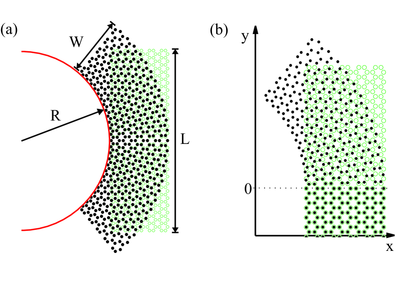
Figure 6: (Color online) (a) Sketch of the strained graphene sheet: we consider a rectangular sample of width $W$ and height $L$, bent into an arc of circle with inner radius $R$. The unstrained graphene sheet is shown as open circles, for comparison. (b) Strain-induced magnetic field barrier step, obtained by bending the graphene lattice only in the $y\geq 0$ region. The number of atoms was reduced in both figures, in comparison to the lattices studied in this work, in order to improve the visualization.

Recently,Guinea2 it was shown theoretically that bending a graphene sheet into an arc of a circle produces a strong and almost uniform pseudo-magnetic field profile. Figure 6(a) illustrates such a strained system, where the rectangular graphene sample of width $W$ and height $L$ is bent into an arc of a circle with inner radius $R$. As the (pseudo) magnetic field points in the same direction (opposite directions) at each $K$ and $K^{\prime}$ points, Vozmediano the combination of both external and strain-induced magnetic field effects provides a valley-dependent magnetic field. If one applies the appropriate external magnetic field for some configuration of the strained graphene, one can obtain an almost perfect suppression of the effective magnetic field at one of the Dirac cones, while the effective field in the other cone is enhanced. This leads to a complicated system to be studied within the Dirac approximation, since one has two completely different systems for the $K$ and $K^{\prime}$ valleys. Namely, Landau levels would be present only around one of the cones (though one cannot expect a perfect Landau level spectrum, since the strain-induced magnetic field is not perfectly uniform in space), whereas in the other cone, the usual continuum spectrum would be observed. This motivated us to analyze the trajectories of a wave packet in such a system within the TB model, where we do not need to include the pseudo-magnetic fields artificially in the Dirac cones, since they appear naturally when we consider the effect of the strain-induced changes of the inter-site distances on the hopping energies, as explained in the previous section.

In this subsection, we investigate the dynamics of a wave packet with width $d=200$ Å  and initial wave vector $k_{x}^{0}=0$ and $k_{y}^{0}=0.02$ Å ^-1 around the Dirac points $K$ and $K^{\prime}$ of Eq. (21) in the presence of external and strain-induced magnetic field barrier steps. As in the $K^{\prime}$ valley the pseudo-spinor $[1,1]^{T}$ is polarized in the negative $y$-direction of the graphene lattice, we choose $[1,-1]^{T}$ for this case, so that a wave packet in this valley will also propagate in the positive $y$-direction. In order to obtain a pseudo-magnetic field barrier step, we consider that the graphene layer is strained only in the $y\geq 0$ region, as sketched in Fig. 6(b). We also consider an external magnetic field $\vec{B}=B\Theta(y)\hat{z}$, where $\Theta(y)$ is the Heaviside step function, which leads to a magnetic barrier step for $y\geq 0$, described by the vector potential $\vec{A}=(-By\Theta(y),0,0)$. In order to avoid effects due to zitterbewegung in the (pseudo) magnetic field region, the wave packet starts at the position $x_{0}=0$, $y_{0}=-420$ Å , so that it can travel for some time in the magnetic field-free region $y<0$ until its velocity converge to a time independent value.

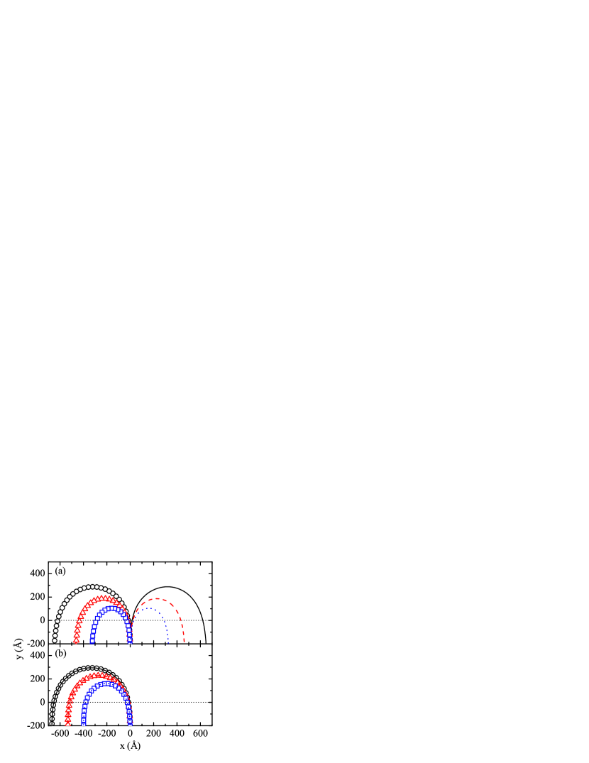
Figure 7: (Color online) Trajectories of the wave packet in the $x-y$ plane, obtained by the TB method for such a system, for initial momentum $k_{y}^{0}=0.02$ Å ^-1 around $K$ (symbols) and $K^{\prime}$ (curves) points, for (a) non-strained graphene with magnetic barrier height $B=5$ T (solid, circles), 7 T (dashed, triangles) and 10 T (dotted, squares), and for (b) a graphene sheet bent into an arc of circle with radius $R=1$ $\mu$m (solid, circles), 0.8 $\mu$m (dashed, triangles) and 0.6 $\mu$m (dotted, squares), considering $B=0$ T. In (b), symbols and curves coincide for each value of $R$.

The influence of the external and strain-induced magnetic field barriers on the trajectories of the wave packet are analyzed separately in Fig. 7, which shows the trajectory of the centroid of the wave packets in $K$ (symbols) and $K^{\prime}$ (curves) points, calculated as $\langle r\rangle=(\langle x\rangle,\langle y\rangle)$, (a) in a non-strained graphene sheet with magnetic field barriers $B=5$ T (solid, circles), 7 T (dashed, triangles) and 10 T (dotted, squares) and (b) in a strained graphene sheet with radius $R=1$ $\mu$m (solid, circles), 0.8 $\mu$m (dashed, triangles) and 0.6 $\mu$m (dotted, squares). All the trajectories form semi-circles in the $y\geq 0$ region, which is due to the Lorentz force produced by the (pseudo) magnetic field. As the external magnetic field (radius of the strained region) increases (decreases), the radii of these semi-circular trajectories are reduced, since a higher (pseudo) magnetic field produces a stronger modulus of the Lorentz force. Notice that the radii of trajectories in the external and pseudo-magnetic fields cases are comparable, which means that for radii $R=1$ $\mu$m - 0.6 $\mu$m of the strained graphene, the generated pseudo-magnetic field is also within $\approx$ 5 T and 10 T. Indeed, the strain induced pseudo-magnetic field distribution for the bend graphene ribbon is given by Guinea2

$$B_{S}(x,y)=-4c\frac{\beta\Phi_{0}}{aL}\arcsin\left(\frac{L}{2R}\right)\cos\left[\frac{2x}{L}\arcsin\left(\frac{L}{2R}\right)\right]$$

$$\times\left[1-\frac{R+y}{L}\arcsin\left(\frac{L}{2R}\right)\right],\hskip 14.22636pt$$ (22)

where $\beta\approx 2$ and $c$ is a dimensionless constant which depends on the details of the atomic displacements. Guinea Considering $L/R\rightarrow 0$ in Eq. (22) the pseudo-magnetic field can be approximated as $B_{S}\approx-c\beta\Phi_{0}\big{/}aR=\omega/R$. Using the value $\omega\approx 4.5\times 10^{4}$ TÅ  estimated numerically in Ref. Low, , one obtains pseudo-magnetic fields within $B_{S}\approx 4.5$ T - 7.5 T for $R=1$ $\mu$m - 0.6 $\mu$m, which are of the same order of magnitude as the external magnetic fields that we considered. For the external magnetic field barrier, the trajectories of wave packets in $K$ and $K^{\prime}$ points form circles in opposite directions, as shown in Fig. 7(a), which is reasonable, since these packets have opposite momentum, which causes a sign change in the Lorentz force. Conversely, considering the strain-induced magnetic barrier illustrated in Fig. 6(b), the trajectories of wave packets in $K$ and $K^{\prime}$ curve in the same direction, since, although their momenta have opposite signs, the pseudo-magnetic fields also point in opposite directions at each Dirac cone $K$ and $K^{\prime}$.

III.3 Strain induced valley filter

Let us consider the strained sample in Fig. 6(b) with $R=1$ $\mu$m. By comparing the radius of the semi-circular trajectory of the wave packet in such a system with those obtained for different intensities of the external magnetic field barrier, one obtains the strain-induced magnetic field for this value of $R$ as $\approx 4.9$ T. Figure 8(a) shows the trajectories in the $x-y$ plane of the centroid of the wave packets in a system where we combine a $R=1$ $\mu$m strain for $y\geq 0$ with an external magnetic field barrier $B=0$ T (solid, open) and 4.9 T (dashed, full), for wave packets in the $K$ (symbols) and $K^{\prime}$ (curves) Dirac points. In the absence of the external magnetic field, both the $K$ and $K^{\prime}$ packets exhibit the same semi-circular trajectory, as discussed earlier. However, when we combine the effect of the strain-induced and external magnetic field barriers, the wave packet in $K^{\prime}$ undergoes a stronger Lorentz force and is readily reflected, whereas the one in the $K$ point performs a practically straight trajectory, as if this packet is not influenced by any Lorentz force. This is a consequence of the fact that combining the effects of a pseudo-magnetic field produced by a $R=1\mu$m strain and a $B=4.9$ T external magnetic field produces a stronger magnetic field in the $K^{\prime}$ point, while in the $K$ point these fields equilibrate, producing a practically magnetic field-free region for particles in this cone. In this situation, the system works as a valley filter, where only wave packets in the $K$ Dirac cone are allowed to pass through the strained region, whereas the wave packets in $K^{\prime}$ are reflected. The results for the wave packet in $K$ for two other values of the external magnetic field are shown as thin solid lines, showing that within a range of $\Delta B=\pm 0.2$ T around $B=4.9$ T, which is a reasonable range for magnetic field intensities in experiments, only a weak Lorentz force is observed and the valley filter works fine.

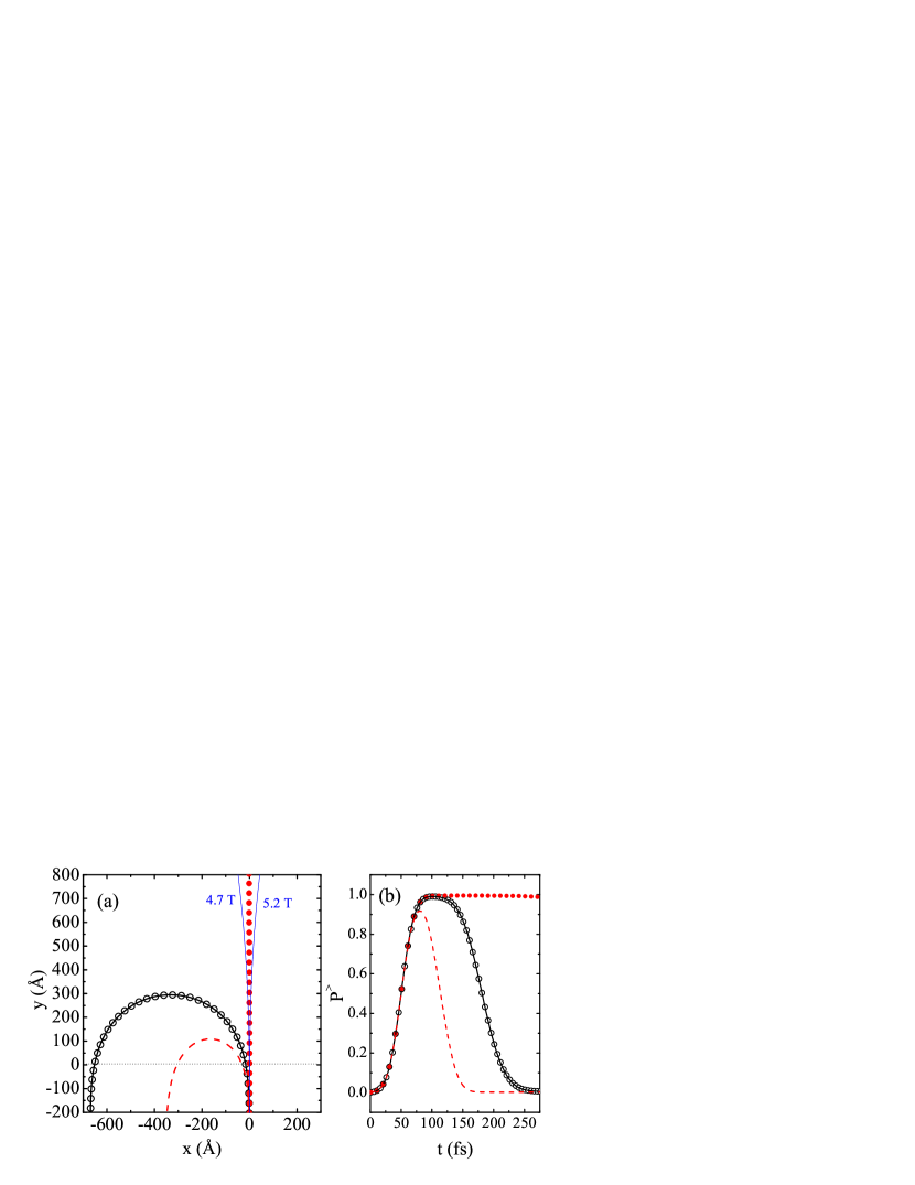
Figure 8: (Color online)(a) Trajectories on the $x-y$ plane for wave packets with initial momentum $k_{y}^{0}=0.02$ Å ^-1 around $K$ (symbols) and $K^{\prime}$ (curves) points, considering a graphene sheet bent into an arc of circle with radius $R=1$ $\mu$m and an external magnetic field $B=0$ T (open, solid) and 4.9 T (full, dashed). The thin solid curves show the results for two other magnetic field intensities for the $K$ packet. (b) Probability of finding the particle in $y\geq 0$ as a function of time, for wave packets with the same configurations as in (a).

The results of Fig. 8 are obtained for both external and pseudo-magnetic field barriers starting at the same position $y=0$. It is straightforward to verify that if there is a mismatch between the starting points of the strained and external field regions, some deviations will occur in the trajectories of the wave packets but, provided the length of the mismatch is much smaller than the magnetic length, the filtering effect is still stable. As an example, a 30 Å  mismatch between the external and pseudo-magnetic field barriers in the system analyzed in Fig. 8 would produce a $\approx$ 5^∘ deviation in the otherwise vertical trajectory of the wave packet in $K$, whereas the wave packet in $K^{\prime}$ is still readily reflected by the combination of magnetic fields in the filter region.

The probability $P^{>}$ of finding the particle in the strained $y\geq 0$ region, calculated as

$$P^{>}(t)=\sum_{n^{>}}\sum_{m}|\Psi_{n,m}^{t}|^{2},$$ (23)

where $n^{>}$ represents the lines of atomic sites with $y\geq 0$, is shown as a function of time in Fig. 8(b). In the $B=0$ T case, both wave packets in $K$ (open circles) and $K^{\prime}$ (solid) stay in the strained $y\geq 0$ region until $t\approx 300$ fs, when they turn back into the $y<0$ region, reflected by the Lorentz force induced by the strain. However, for $B=4.9$ T, $P^{>}$ already approaches zero at $t\approx 175$ fs for the packet in $K^{\prime}$ (dashed), whereas for $K$ (full circles), it remains close to 1 even for large $t$.

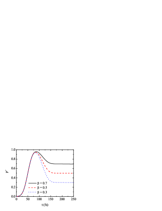
Figure 9: (Color online) Probability of finding the electron in the filter region $y\geq 0$, for an initial wave packet given by a combination of Gaussian distributions around both $K$ and $K^{\prime}$ Dirac points, for three different values of the $K$-component of the wave packet $\beta$.

The efficiency of the proposed valley filter is confirmed by Fig. 9, where we present $P^{>}$ as a function of time for initial wave packets given by a combination of Gaussians around the $K$ and $K^{\prime}$ points in Eq. (21):

$$\Psi=\sqrt{\alpha}\Psi_{K^{\prime}}+\sqrt{\beta}\Psi_{K},$$ (24)

where $\Psi_{K(K^{\prime})}$ is the Gaussian wave packet in Eq. (18) with momentum $\vec{q}$ around the $K(K^{\prime})$ Dirac point. The results are presented for three different values of $\beta$, where one can easily see that the probability of finding the packet in the strained region exhibits a peak at $t\approx 80$ fs but, as the $K^{\prime}$ part of the packet is reflected by the magnetic barrier, this probability decays, reaching exactly $P^{>}=\beta$ for large $t$. Such a system proves to be a perfect valley filter, which is able to reflect all the components of the incoming packet that are in the $K^{\prime}$ point and transmit a wave packet that is composed only of particles with momentum in the vicinity of $K$.

We point out that when a wave packet reaches the edges of a graphene nanoribbon, it can be scattered to a different Dirac cone. Chen Consequently, the efficiency of the valley filter could be compromised if one considers a thin nanoribbon, so that the filtered wave packet could still reach its boundaries and scatter back to the other valley. In order to avoid such an effect, we have considered a wide nanoribbon, so that for the time intervals we study in this work, boundary effects are not significant.

III.4 External and pseudo magnetic field effects on the zitterbewegung

In a previous paper, Rusin and Zawadzki Rusin1 used the Dirac Hamiltonian for graphene to show that the zitterbewegung, which is transient for $B$ = 0, as discussed earlier, is permanent for $B\neq 0$. Furthermore, the authors showed that for a Gaussian wave packet, the time evolution of the average value of the current is different in $x$ and $y$ directions, which they explain as due to the fact that the Dirac Hamiltonian is not symmetric in the momenta $\hat{p}_{x}$ and $\hat{p}_{y}$. Although the same authors say in their subsequent paper Rusin2 that this effect is unphysical, because it violates the rotational symmetry of the $x-y$ graphene plane, we believe this result is still physical: one must remember that the Dirac model of graphene comes from the tight-binding approach for this system, which describes a honeycomb lattice of atoms that is not symmetric in the $x-y$ plane by definition, exhibiting C_6v symmetry, as mentioned in previous section. For each $K$ and $K^{\prime}$ point, the coordinates x and y in the Dirac Hamiltonian represent different directions in the real honeycomb lattice of graphene, where for an infinite sample the x (y) coordinate in the Dirac equation is related to one of the zigzag (armchair) directions of the real sample. In this subsection, we use our TB model of graphene to extend the previous study of Rusin and Zawadzki Rusin1 to different situations.

We now study the dynamics of a wave packet with width $d=200$ Å , pseudo-spinor $c_{1}=1$ and $c_{2}=1$ and initial wave vector $k_{x}^{0}=k_{y}^{0}=0$, i.e. exactly at one of the Dirac points $K$ and $K^{\prime}$ in Eq. (21), in the presence of an uniform applied external magnetic field $\vec{B}=B\hat{z}$, instead of the magnetic field barrier step considered in the previous subsection. We also consider a pseudo-magnetic field obtained by bending the whole rectangular graphene sample into an arc of a circle with radius $R$, as illustrated in Fig. 6(a). The radius of the circle is considered as $R=1$ $\mu$m, which produces a $\approx 4.9$ T pseudo-magnetic field, as demonstrated in the previous subsection. Accordingly, we consider the external uniform magnetic field as $B=4.9$ T.

A few experimental techniques have been suggested in the literature for the observation of zitterbewegung. Schliemann ; Gerritsma An interesting one Rusin2 is based on the fact that the wave packet $\Psi(\vec{r},t)$ exhibits an electric dipole moment $\vec{D}(t)=\langle\Psi(\vec{r},t)|\vec{r}|\Psi(\vec{r},t)\rangle$ and, consequently, the zitterbewegung yields an oscillation of this dipole moment, which is a source of electromagnetic radiation, described classically Jackson by the equation

$$\vec{\varepsilon}(t)=\frac{d^{2}\vec{D}(t)}{dt^{2}}\frac{\sin{\Phi}}{4\pi\epsilon_{0}s},$$ (25)

where $s$ and $\Phi$ are the distance and angle of observation, respectively, and $\epsilon_{0}$ is the vacuum permittivity.

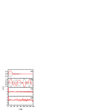
Figure 10: (Color online) Electromagnetic dipole radiation as a function of time for wave packets with initial pseudo-spinor $[1,1]^{T}$ at $K$ (thin curves) and $K^{\prime}$ (thick curves), considering a graphene sheet (a) in the absence of strain and magnetic fields, (b) under an uniformly applied magnetic field $B=4.9$ T, (c) bent into an arc of circle with radius $R=1\mu$m (see Fig. 6) and (d) with both the uniform magnetic field $B=4.9$ T and the $R=1\mu$m bending. Solid (dashed) curves are the results for the $\varepsilon_{y}$ ($\varepsilon_{x}$) component.

Figure 10 shows the effects of external and strain-induced magnetic fields on the electric field radiation produced by the zitterbewegung, written in units of $\varepsilon_{c}=\sin{\Phi}\big{/}4\pi\epsilon_{0}s$. Only weak oscillations are expected in the armchair ($x$) direction, since the pseudo-spin $[1,1]^{T}$ points in the x-direction in the Dirac model which, as mentioned earlier, is related to the zigzag ($y$) direction of the honeycomb lattice. Indeed, in Fig. 10(a-d), the $x$-component of the electric field (dashed) is always close to zero. In Fig. 10(a), we present the results in the absence of strain and magnetic fields, for comparison. In this case, the oscillations on the electric field are suppressed for larger time, which is due to the transient character of the zitterbewegung. Besides, the results for $\varepsilon_{y}$ (solid) in the $K$ (thin curves) and $K^{\prime}$ (thick curves) points have opposite signs, since for these points the axis of the Dirac cones are rotated by angles which differ by $\pi/2$ difference. In Fig. 10(b), the uniformly applied magnetic field $B=4.9$ T in an unstrained sample leads to persistent oscillations in $\varepsilon_{y}$, which is related to the discrete Landau level spectrum created by this field. Each Landau level that is populated by the Gaussian distribution contributes with a different frequency. Rusin1 Figure 10(c) shows that such a persistent behavior is also obtained by bending the graphene sheet into an arc of circle with radius $R=1\mu$m, which produces a pseudo-magnetic field of the same order of magnitude. Notice that the amplitude of oscillations in this case is four times smaller than those found in Fig. 10(b) for the unstrained sample under an external magnetic field. In fact, these two cases are not expected to produce the same zitterbewegung, because, although both samples exhibit approximately the same magnitude of magnetic field, the strained sample has not only the pseudo-magnetic field, but also a different distribution of atomic sites. Thus, in the strained case, there is an additional change in the direction of the pseudo-spin polarization as the wave packet drifts, due to the lattice distortion itself. As we have demonstrated in Sec. III A, the zitterbewegung strongly depends on the pseudo-spin polarization and hence, the different interplay between the strained atomic sites and the initial pseudo-spin polarization produces a different zitterbewegung for the strained case, as compared to the one of the unstrained sample under an external field.

In Fig. 10(d), we combine the effects of the $R=1$ $\mu$m strain and $B=4.9$ T external field to produce a system where the magnetic field is practically zero in the $K$ point, but is non-zero in the $K^{\prime}$ point, so that only the packet in the $K^{\prime}$ point exhibits persistent oscillations. For the $K$ point, the external field compensates only the effect of the pseudo-magnetic field, namely, the persistent zitterbewegung, but it does not remove the effect of the lattice distortion. As a result, comparing the results for $K$ (thin curves) in Figs. 10(a) and (d), one observes that the oscillations are transient in both cases, since there is no effective magnetic field, but they still exhibit a different oscillation profile at small $t$, due to the lattice distortion in the latter case, which is absent in the former.

IV Conclusion

We presented a study of the dynamics of Gaussian wave packets in graphene under external and strain-induced magnetic fields, where the latter is obtained by bending the graphene sheet into an arc of a circle. The dependence of the zitterbewegung on the initial pseudo-spin of the wave packet is investigated, and the results obtained by means of the tight-binding model and the Dirac equation are compared. We demonstrate that the combination of the pseudo-magnetic field, induced by bending the graphene sheet, along with an external magnetic field with appropriate strength can be used as an efficient valley filter. An incoming wave packet composed of momenta around the $K$ and $K^{\prime}$ Dirac points is scattered such that all its components in one of the Dirac cones undergoes a strong Lorentz force and are readily reflected, while the components in the other cone are allowed to pass through the device with only small distortions in their trajectory, due to the very weak residual Lorentz force.

Our results also show that in the absence of external or strain-induced magnetic fields, the zitterbewegung is a transient effect, whereas in the presence of any of these fields, the oscillations persist in time. In a strained sample under an external magnetic field with the appropriate strength, the effective magnetic field in one of the Dirac cones is enhanced, whereas in the other cone it is practically cancelled. In this situation, a permanent zitterbewegung is observed only for wave packets in one of the Dirac cones. The wave packet oscillations produce electric field radiation, which can be detected experimentally.

Finally, we believe the present work contributes to a better understanding of the relation between the results obtained from TB and Dirac approaches for graphene and those to be observed in future experiments on strained graphene-based structures.

- (1) K. S. Novoselov, A. K. Geim, S. V. Morozov, D. Jiang, Y. Zhang, S. V. Dubonos, I. V. Grigorieva, and A. A. Firsov, Science 306, 666 (2004).
- (2) A. H. Castro Neto, F. Guinea, N. M. R. Peres, K. S. Novoselov, and A. K. Geim, Rev. Mod. Phys. 81, 109 (2009).
- (3) B. Thaller, arXiv:quant-ph/0409079v1 (2004).
- (4) W. Zawadzki, T. M. Rusin, Phys. Lett. A 374, 3533 (2010).
- (5) G. Dàvid and J. Cserti, Phys. Rev. B 81, 121417(R) (2010).
- (6) E. Schrödinger, Sitzungsber. Preuss. Akad. Wiss. Phys. Math. Kl. 24, 418 (1930).
- (7) W. Zawadzki, Phys. Rev. B 72, 085217 (2005).
- (8) J. Schliemann, D. Loss, and R. M. Westervelt, Phys. Rev. Lett. 94, 206801 (2005).
- (9) T. M. Rusin and W. Zawadzki, Phys. Rev. B 80, 045416 (2009).
- (10) Y.-X. Wang, Z. Yang, and S.-J. Xiong, Europhys. Lett. 89, 17007 (2010).
- (11) R. Gerritsma, G. Kirchmair, F. Zähringer, E. Solano, R. Blatt, and C. F. Roos, Nature (London) 463, 68 (2010).
- (12) V. M. Pereira and A. H. Castro Neto, Phys. Rev. Lett. 103, 046801 (2009).
- (13) Seon-Myeong Choi, Seung-Hoon Jhi, and Young-Woo Son, Phys. Rev. B 81, 081407(R) (2010).
- (14) F. M. D. Pellegrino, G. G. N. Angilella, and R. Pucci, Phys. Rev. B 81, 035411 (2010).
- (15) O. Bahat-Treidel, O. Peleg, M. Grobman, N. Shapira, M. Segev, and T. Pereg-Barnea, Phys. Rev. Lett. 104, 063901 (2010).
- (16) T. Fujita, M. B. A. Jalil, and S. G. Tan, Appl. Phys. Lett. 97, 043508 (2010).
- (17) Z. Wu, F. Zhai, F. M. Peeters, H. Q. Xu and K. Chang, arXiv:1008.4858v3 (2010).
- (18) E. Cadelano, S. Giordano, and L. Colombo, Phys. Rev. B 81, 144105 (2010).
- (19) G. Cocco, E. Cadelano, and L. Colombo, Phys. Rev. B 81, 241412 (2010).
- (20) Y. Lu and J. Guo, Nano Res. 3, 189 (2010).
- (21) M. A. H. Vozmediano, M. I. Katsnelson, and F. Guinea, Phys. Rep. 496, 109 (2010).
- (22) F. Guinea, M. I. Katsnelson, and A. K. Geim, Nat. Phys. 6, 30 (2010).
- (23) T. Low and F. Guinea, Nano Lett. 10, 3551 (2010).
- (24) F. Guinea, A. K. Geim, M. I. Katsnelson, and K. S. Novoselov, Phys. Rev. B 81, 035408 (2010).
- (25) N. Levy, S. A. Burke, K. L. Meaker, M. Panlasigui, A. Zettl, F. Guinea, A. H. Castro Neto, M. F. Crommie, Science 329, 544 (2010).
- (26) G. M. Maksimova, V. Ya. Demikhovskii, and E. V. Frolova, Phys. Rev. B 78, 235321 (2008).
- (27) T. M. Rusin and W. Zawadzki, Phys. Rev. B 78, 125419 (2008).
- (28) E. Romera and F. de los Santos, Phys. Rev. B 80, 165416 (2009).
- (29) V. Krueckl and T. Kramer, New J. Phys. 11, 093010 (2009).
- (30) A. Rycerz, J. Tworzydło, and C. W. J. Beenakker, Nat. Phys. 3, 172 (2007).
- (31) A. Weisse, G. Wellein, A. Alvermann, and H. Fehske, Rev. Mod. Phys. 78, 275 (2006).
- (32) S. Mahapatra and N. Sathyamurthy, J. Chem. Soc. 93, 773 (1997).
- (33) R. Kosloff, J. Phys. Chem. 92, 2087 (1988).
- (34) A. Chaves, G. A. Farias, F. M. Peeters, and B. Szafran, Phys. Rev. B 80, 125331 (2009).
- (35) D. A. Bahamon, A. L. C. Pereira, and P. A. Schulz, Phys. Rev. B 79, 125414 (2009).
- (36) M. Governale and C. Ungarelli, Phys. Rev. B 58, 7816 (1998).
- (37) V. M. Pereira, A. H. Castro Neto, and N. M. R. Peres, Phys. Rev. B 80, 045401 (2009).
- (38) N. Watanabe and M. Tsukada, Phys. Rev. E 62, 2914 (2000).
- (39) J. M. Pereira, A. Chaves, G. A. Farias, and F. M. Peeters, Sem. Sci. Tech. 25, 033002 (2010).
- (40) H. N. Nazareno, P. E. de Brito, and E. S. Rodrigues, Phys. Rev. B 76, 125405 (2007).
- (41) J.-H. Chen, W. G. Cullen, C. Jang, M. S. Fuhrer,and E. D. Williams, Phys. Rev. Lett. 102, 236805 (2009).
- (42) J. D. Jackson, Classical Electrodynamics (Wiley, New York, 1975).