A powerful computational crystallography method to study ice polymorphism

Abstract

Classical Molecular Dynamics (MD) simulations are employed as a tool to investigate structural properties of ice crystals under several temperature and pressure conditions. All ice crystal phases are analyzed by means of a computational protocol based on a clustering approach following standard MD simulations. The MD simulations are performed by using a recently published classical interaction potential for oxygen and hydrogen in bulk water, derived from neutron scattering data, able to successfully describe complex phenomena such as proton hopping and bond formation/breaking. The present study demonstrates the ability of the interaction potential model to well describe most ice structures found in the phase diagram of water and to estimate the relative stability of sixteen known phases through a cluster analysis of simulated powder diagrams of polymorphs obtained from MD simulations. The proposed computational protocol is suited for automated crystal structure identification.

I Introduction

Many attempts have been performed to reproduce the complex phase diagram of water, in particular the ice polymorphs, by means of classical Molecular Dynamics (MD) malenkov_zheligovskaya ; guillot2002reappraisal ; sanz-vega ; bartok_2005 . Since MD is essentially based on the evolution of an exact configuration of atoms in phase space, water is usually treated in a peculiar way because of the non purely classical behavior of hydrogen. Most classical interaction potentials treat the water molecule as a rigid body composed of three single point charges (i.e. SPC), not allowing, or significantly reducing, the degrees of freedom associated to the hydrogen atoms. This approximation is acceptable only when the focus is not on the hydrogen atoms themselves, with water molecules supposed to be perfectly stable and no proton dynamics expected. Some other potentials are based on more complex approximations which add bond flexibility to the water molecule (i.e. SPC and TIP4P variants). However, all such classical force fields are unable to quantitatively describe hydrogen diffusion. A variety of potentials for water is presently available, and for a list of them see the review by Guillot guillot2002reappraisal and references therein. In the literature, the most used potentials for ice simulations are the TIP4P and SPC/E potentials sanz-vega ; bartok_2005 .

To date, the most systematic MD investigations on the relative stability of ice phases are the work of Zheligovskaya Zheligovskaya , based on the potential of Poltev-Malenkov poltev-malenkov , and that of Baranyai et al. bartok_2005 , which uses SPC/E and TIP4P water models. From such investigations, it is clear that the used model potentials are not able to reproduce all sixteen known crystal structure of ice. Inaccuracy of current potentials, and the rigidity imposed on the water molecule are considered the main reasons for this failure Zheligovskaya ; parrinello ; bartok_2005 , confirming that for an adequate description of the ice and/or water systems by classical MD, the quality of the potential is of prime importance.

Earlier, some of the authors of this study introduced a new reactive force field for water (RWFF)hofmann-r-potential , which was derived from neutron scattering data. This force field, while of classical nature, allows proton diffusion by a breaking/reforming mechanism of O-H bonds in water molecules, in acids and in hydronium ions, and correctly describes the proton dynamics and the structure of bulk water. The RWFF has been extensively and successfully applied to the theoretical investigation of conductivity in polyelectrolyte membranes for fuel cellshofmann_fc ; hofmann_conduct .

In this study, and by using the RWFF potential, several MD simulations have been carried out by encompassing the range of pressure, $P$, and temperature, $T$, needed to analyze all crystal phases of water. The so obtained crystal structures are then ready to be fully characterized in their structure.

A large amount of publications is also dedicated to the development of efficient methods able to characterize and classify the different ice structures. Extensive studies on ice classification have been made by Chaplinm_chaplin and Malenkovmalenkov2009 . The used approach is based on the detection of different local topologies of the bond network such as proton disorder/order, ring sizes, helices, angles, and ring penetration. The crystal structures are then compared pairwise according to the different properties. However, such a procedure is not well suited for an automated classification analysis.

Other complex classification criteria have been introduced to analyze water structures and ice polymorphs obtained during MD simulations. Carignano et al.carignano looked at the time average of the number of H-bonds around O-atoms to detect different phases of water and ice Ih. Moore and Molinaromoore_2009 developed an algorithm which focuses on the first coordination sphere of each oxygen, where any deviation from perfect tetrahedrality classifies water molecules as belonging to the liquid or to the solid phase in two clusters. This algorithm has been extended to recognize water molecules belonging to Ih or Ic structures moore_2010 .

An alternative method is based on the analysis and classification of the crystal structures by means of their clustering in the reciprocal space hofmann-similarity . Ice crystal structures can hardly be compared in the direct space, since the presentation of the unit cell is not unique, and small changes of the lattice can easily be missed. However, a Fourier transform of the real coordinates gives an unique presentation for each phase, while the multiplication of the Fourier transform with the scattering factors results in the powder diagrams. In the present study, the powder diagrams are generated for samples obtained in MD simulations and then used to classify the ice crystal structures.

Clustering techniques rely on the definition of a similarity index capable of reducing to a single number many relevant geometrical properties. Such techinques, have already been defined and employed for the estimation of the number of local minima within the energy landscape of crystal structures hofmann-minima and for automated crystal structure determination hofmann-automated . In this way, a quick and univocal detection of manifold and isostructural crystal structures in extensive data sets data-mining was possible. In the present work, the similarity index introduced in Hofmann et al. hofmann-similarity has been employed and more details on its definition can be found there. For our purposes, we recall that this index is based on comparing integrated powder diffraction diagrams instead of the powder diagrams themselves. The index is defined as the mean difference between two normalized integrated powder diagrams and is proportional to the area between the two curves. In contrast to traditionally used similarity indices, this method is valid for comparisons where large deviations of cell constants are present.

In this work the method is applied to identify the different crystal structures of ice, outcomes of long MD simulations over a broad range of temperature and pressure.

The paper is organized as follows: In Section 2 the phase diagram of water and a classification of all known ice crystal structures are presented. Section 3 is dedicated to the illustration of the crystal clustering analysis and of the proposed computational crystallography protocol. The protocol is established with the aim to accurately verify the ability of the RWFF potential of reproducing the stability of the ice crystal structures found in each point of the thermodynamical phase diagram. Molecular Dynamics details needed to perform the simulations are reported in Section 4. The results of the computational crystallography protocol are shown and discussed at length in Section 5. The last Section is dedicated to the conclusions.

II Taxonomy of ice structures

At present, sixteen crystal morphologies of ice are known within the water phase diagram over a very broad range of temperature and pressure. The different ice phase regions and structures are shown in Figure 1. Most of the ice modifications are characterized by specific regions of stability, while some others (Ic, IV, XII) occur exclusively as metastable states.

Some crystallographic information concerning ice polymorphs is summarized in Table 1. Water crystallizes in different space groups and the density of each structure varies over a broad range from $0.930$ to $2.785$ g/cm³ (sixth column of Table 1). The crystallographic densities are reported in this table and they can be slightly different from the experimental values due to the presence of crystal defects in real samples (e.g. vacancies, interstitials, etc.) The number of molecules in the asymmetric cell ranges from 1/2 to 7 (column Z’), while the number of molecules in the unit cell goes from 2 up to 28 (column Z). According to the H atom positions (water molecules orientation), proton ordered and proton disordered phases are defined (column o/d). Some of these phases differ just because of proton order/disorder malenkov2009 .

Table 1 reports the configurational energy (sum of RWFF and of the electrostatic terms) for most of the structures obtained in this work and a comparison with two widely used force fields for water.

In the structures of all known polymorphs of ice, with the only exception of ice X, each water molecule forms four hydrogen bonds with neighbor molecules. In ice X each proton does not belong uniquely to a single oxygen atom, but it is shared between two oxygens. This fact leads to a quantum behavior that can only be approximately described by means of a standard MDparrinello-iceX .

The “low pressure” phases (Ih, Ic, XI) are characterized by a nearly ideal tetrahedral environment of the oxygen atoms, while “medium and high pressure” phases (II-IX, XII-XV) show a more or less distorted tetrahedral coordination of the oxygens.

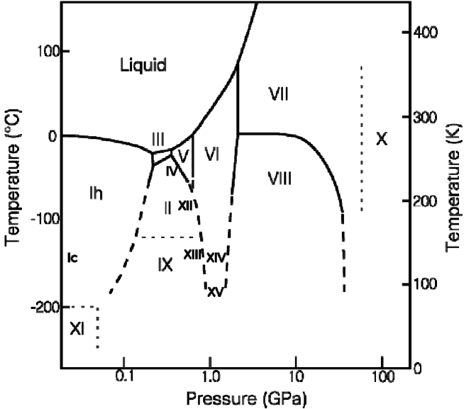
Figure 1: Phase diagram of water lobban1998structure . Ice IV, XII, XIII, XIV, XV (not included in the original diagram) are placed near their known stability regions.

Table 1: Characteristics of ice structures. $\Delta U_{pot}$ is computed by subtracting from the energy of each structure the energy of the most stable (ice XI.) Data relative to TIP4P and SPC/E taken from Vega et al.vega-gdr1 and Martin-Conde et al.vega-gdr2

structure	o/d	space group	Z’	Z	$\rho$ (g$\cdot$ cm-3)	$\Delta U_{pot}$(kJ/mol) RWFF	TIP4P	SPC/E
Ic	d	$Fd\overline{3}m$	0.5	8	0.933	1.31	1.92	2.13
Ih	d	$P6_{3}/mmc$	1	4	0.926	9.65	7.19	7.53
II	o	$R\overline{3}$	2	12	1.195	6.67	4.18	2.13
III	d	$P4_{1}2_{1}2$	1.5	12	1.160	9.76	8.49	8.83
IV	d	$R\overline{3}c$	2	16	1.275	8.69	5.52	6.02
V	d	$C2/c$	4	28	1.233	15.36	7.78	8.45
VI	d	$P4_{2}/nmc$	1.5	10	1.314	14.17	8.20	9.20
VII	d	$Pn\overline{3}m$	0.5	2	1.591	27.50	7.78	8.45
VIII	o	$I4_{1}/amd$	1	8	1.885	21.61	8.95	10.12
IX	o	$P4_{1}2_{1}2$	1.5	12	1.160	2.26	4.68	4.31
X	nm	$Pn\overline{3}m$	0.5	2	2.785	171.70	-	-
XI	o	$Cmc2_{1}$	1.5	8	0.930	0.00	0.00	0.00
XII	d	$I\overline{4}$	1.5	12	1.301	10.54	9.45	10.21
XIII	o	$P2_{1}/c$	7	28	1.247	8.16	3.76	3.22
XIV	o	$P2_{1}2_{1}2_{1}$	3	12	1.294	6.91	3.47	4.18
XV	o	$P\overline{1}$	5	10	1.328	7.09	-	-

III Crystal clustering analysis and computational crystallography protocol

To verify the accuracy of the RWFF potential in describing all the sixteen ice structures reported in the previous Section, the following “computational crystallography protocol” is adopted:

1. Make a choice of a thermodynamic point;

2. Perform MD simulations by starting from the ideal crystal structures, and store the final thermalized crystal structures;

3. Compute the powder diffraction diagrams for the initial and for the equilibrated ice structures, then evaluate the corresponding similarity indices;

4. Cluster the structures, and draw the dendrogram as obtained from the average linkage distance.

When the final structures of the MD simulations cluster with the starting ideal crystal structures, the force field is able to mantain structural stability.

In this Section and to give an example of such a protocol, the dendrogram obtained for all ice structures from published theoretical crystal data ICSD is evaluated.

Since in this case step 1 and 2 are not required, the protocol starts from step 3. For the step 3, the calculation of powder diffraction diagrams and of their clustering for all ice structures was done with FlexCryst software flexcryst . Here, it is stressed that the clustering approach helps to visualize, in a single picture, the complex relations existing within the crystal structure set, and to intuitively understand the influence of temperature and pressure. The results of step 4 are reported in Fig. 2, where the powder diagrams of the ideal crystal structures (upper part), and the result of the clustering operation on them (lower part), are shown.

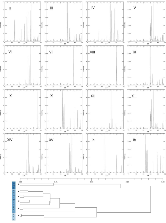
Figure 2: Powder diagrams of the ideal crystal structures and their dendrogram. Asterisks indicate ordered-disordered crystal couples (darker shades of blue correspond to stability at higher pressures.)

The dendrogram reveals three structural clusters, making visible a taxonomy ruled by pressure effects: The crystal structures split in a “low pressure” cluster with the polymorphs Ih, Ic, XI; a “medium pressure” cluster with the polymorphs II-VI, IX and XII-XV; and a “high pressure” cluster with ice VII, VIII, X. Within these clusters, and in agreement with the data summarized in a recent paper by Malenkovmalenkov2009 , one can easily spot the proton ordered-disordered couples of structures (marked by asterisks in the dendrogram), even if they belong to different space groups: Ih-XI, III-IX, V-XIII, VI-XV, VII-VIII, XII-XIV.

In the rest of the paper the protocol will be used in its full extension.

IV Molecular Dynamics simulations

For the MD simulations, it has been used a customized version of DL$\_$POLY V.2 DLPOLY modified in order to include the reactive water force field, RWFF hofmann-r-potential . The RWFF potential, which was derived to reproduce correctly liquid water neutron scattering data over a broad range of temperatures and pressures hofmann-r-potential , and which has been employed in the present study, is shown in Fig. 3. It is only available in a tabular form which is automatically interpolated by DL$\_$POLY.

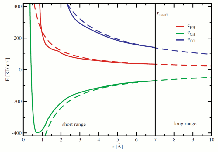
Figure 3: The graphical representation of the RWFF potentials. The short range potentials are shown in full lines. After the cutoff at 7 Å  the potentials are continued by the Coulomb terms (dashed lines).

IV.1 Initial configurations

For each ice structure, a supercell with 1680 water molecules has been generated by repeating the unit crystal cell along the three spatial dimensions. Hereby, the supercell was constrained to an approximately cubic shape. The atomic coordinates were taken from the Inorganic Crystal Structure Database, (ICSD) ICSD . The size of the supercell is a compromise to minimize finite-size effects and CPU-time. The number 1680 is the least common multiple of the different numbers of molecules in the unit cells of the polymorphs. Therefore, such a supercell can be used for all of them. For the cases in which the hydrogen positions were experimentally undefined, the hydrogen atoms have been placed by following the Bernal-Fowler rules bernal-fowler : This freedom in configuration building is due to the use of the RWFF model which allows to place the hydrogen atoms anywhere in the lattice.

IV.2 Details of MD simulations

The initial configurations, generated as described in the above subsection, were then equilibrated by MD run within the isothermal-isobaric ensemble (NPT), in which the number of atoms, the pressure and the temperature have been kept constant during the simulation. Real space cutoff for the RWFF interaction was set to $7.0$ Å while for the long range Coulomb part, a full Ewald summation was employed. An anisotropic Nosé-Hoover barostat and thermostat has been employed with a time constant of $0.4$ ps. In this way the simulation box is free to optimize both its volume and its shape. Pressure and temperature do not show any drift or long period oscillations during the simulations. The timestep was set to $0.1$ fs, which is smaller than common MD simulations for water. This small timestep is necessary to describe accurately the fast vibrations of the protons and to conserve total energy over long time scales. Each simulation was evolved for $1.0\cdot 10^{6}$ steps using a Verlet algorithm verlet , so that the total time reached 100 ps.

After the equilibration run in NPT ensemble, every sample was evolved for further 100 ps ($1.0\cdot 10^{6}$ simulation steps) in the microcanonical ensemble (NVE) with constant number of atoms, volume and internal energy. During the NVE run the energy has always been conserved within $0.1\%$ over $1.0\cdot 10^{6}$ steps. The NVE ensemble avoids any artificial effect due to the thermostat and the barostat action, important when studying dynamical properties.

V Results and Discussion

V.1 The ice polymorphs at different conditions

To detect structural changes of the ice phases at different thermodynamical conditions, the following three sets of (T, P) points in the phase diagram of water were selected: a) a set of points (16 points) located near the middle of the stability region of each polymorph (as explained later, for ice IV and VI it was necessary to modify the initial guess of the stable zone); b) a point at T=$150$ K and P=$1$ MPa; c) a point at T=$150$ K and P=$1$ TPa. For the b) and c) points all sixteen ice structures are simulated. In the following, the a) set will be usually referred to as “native conditions”, the b) point as “low pressure” and the c) point as “high pressure”.

In Table 1 the last three columns contain the energy difference between every structure and the most stable one, which happens to be always ice XI for the three force fields consideredvega-gdr1 ; vega-gdr2 . Absolute values would have been difficult to directly compare because RWFF contains the intramolecular bond energy which is naturally not present for TIP4P and SPC/E. The relative energy ordering for RWFF is not so different from the other two force fields and we immediately note that, apart from ice XI (the lowest configurational energy structure), the second lowest energy is cubic ice and the others follow a similar trend. The energies for high pressure ices (V, VI, VII, VIII) show very high values for RWFF with respect to the rigid models. This is explained by the fact that O-H intramolecular distances are shorter and this part of the interaction dominates in compressed water molecules. This is confirmed by an analysis of the radial distribution functions. Ice X shows an extremely high $U_{pot}$ value because the H atoms stay in a shared lattice position between two oxygens.

V.2 Native conditions

Following the MD procedure described above, the relaxation of every ice structure has been performed within the characteristic region of stability on the phase diagram (Figure 1). The corresponding values of temperature and pressure, see Table 2, have been taken approximately in the middle of each stability zone. With this choice, the powder diagrams of the equilibrated structures have then been calculated, and each powder diagram has been compared with the one of the corresponding ideal structure reported in Table 1, in order to reveal possible structural changes. The powder diagrams for most polymorphs were found substantially identical for both the initial configuration and the final configuration after equilibration.

Table 2: Temperature and pressure of the chosen thermodynamics states

structure	Ic	Ih	II	III	IV	V	VI	VII
T (K)	130	250	200	250	110	250	225	350
p (GPa)	$10^{-7}$	$10^{-7}$	0.30	0.30	$10^{-7}$	0.53	1.50	10.00
structure	VIII	IX	X	XI	XII	XIII	XIV	XV
T (K)	150	50	150	50	180	130	120	100
p (GPa)	10.00	0.30	100.00	$10^{-7}$	0.81	0.50	1.20	1.10

The only difference observable between the initial and post MD powder diagrams is the background noise. In fact, the equilibrated structures differ slightly from the ideal ones as a result of small lattice deformations at different length scales. We observed two different effects of this phenomenon: most structures show just thermal noise with average positions equal to the ideal ones, on the other hand, a few of them (i.e. ice V and XIII in Fig. 6) thermalize into imperfect lattices. This (stable) distortion is easily detectable in the powder diffraction diagrams as a low but broad bulge centered on the main peaks. On the other hand, as an example of pure thermal lattice distortion, Fig. 4 shows that for ice Ih the noise has a very low intensity, it is more uniformly distributed over the powder diagram and should average out to zero in the limit of an infinite system.

The difference between the initial and the post MD structures is quantified by the distance in average linkage, graphically represented in the dendrograms. This adimensional quantity should be used as a relative similarity index: the nearer to the left on the dendrogram two structures are connected, the higher will be their structural similarity.

As an example, the pictures of ice Ih before and after equilibration are shown in Fig. 4 (left part: top and bottom). At $0$ K the structure is ideal and the powder diagram is free of noise (top right of Fig. 4). The snapshot of the structure at $250$ K shows some random molecular displacements. As can be seen in the direct space as well as in the reciprocal space (bottom right), the structure remains stable. To further check the geometrical structure of ice Ih after the MD at $T=250$ K and $P=0.1$ MPa, we plotted in Fig. 5 the oxygen-oxygen radial distribution function for the RWFF, for the experimental data (Sopersoper ) and for TIP4P (taken from Vega et al.vega-gdr1 .) It should be noted that Soper data was obtained at $T=220$ K. The most striking difference between the MD curves and the experimental one is the presence of two small peaks, one on the left and one on the right, of the first big peak at about $2.8$ Å. This value for the nearest neighbor distance agrees well with the experimental one reported by Kuhs and Lehmannkuhs-lehmann . Moreover, the second peak of the radial distribution function, from which we can compute the O-O-O angle, corresponds to an angle of about $107$ degrees, which is also in good agreement with the data reported in the previously cited reference kuhs-lehmann . A detailed comparison such as the one reported in Morse and Rice morse-rice would be interesting, but it is beyond the scope of this paper. The agreement between our data and the experimental one is of the same degree of accuracy as TIP4P or even better. Since the RWFF was obtained by fitting exclusively experimental liquid water radial distribution functions, we believe that the model is capturing a fair amount of water physics with a spherically symmetric interaction. We should recall once more that RWFF is totally flexible having no proper “bonded interactions” versus the constrained geometry of the other models. This fact makes even more remarkable the fact that we are able to simulate stable complex structures such as ice X for such long times.

From this systematic analysis it turns out that the reactive water force field (RWFF) generates stable ice structures under experimental conditions with the exception of ice IV and VI. Ice IV and VI collapsed into amorphous states due to the fact that their stability regions are very narrow and not well defined, making it difficult to choose the reference thermodynamic points characterizing such phases. In the paper by Vega et al.vega-gdr1 the used temperatures and pressures to simulate these two structures are different from experimental values and it turned out that, by using their pressure values (for ice VI we had to increase pressure by $0.4$ GPa with respect to the experimental value, while for ice IV pressure was set to $0.1$ MPa), stable structures were achieved with both isotropic and anisotropic barostats. Please note that T and P reported in Table 2 are those for which we obtained stable structures.

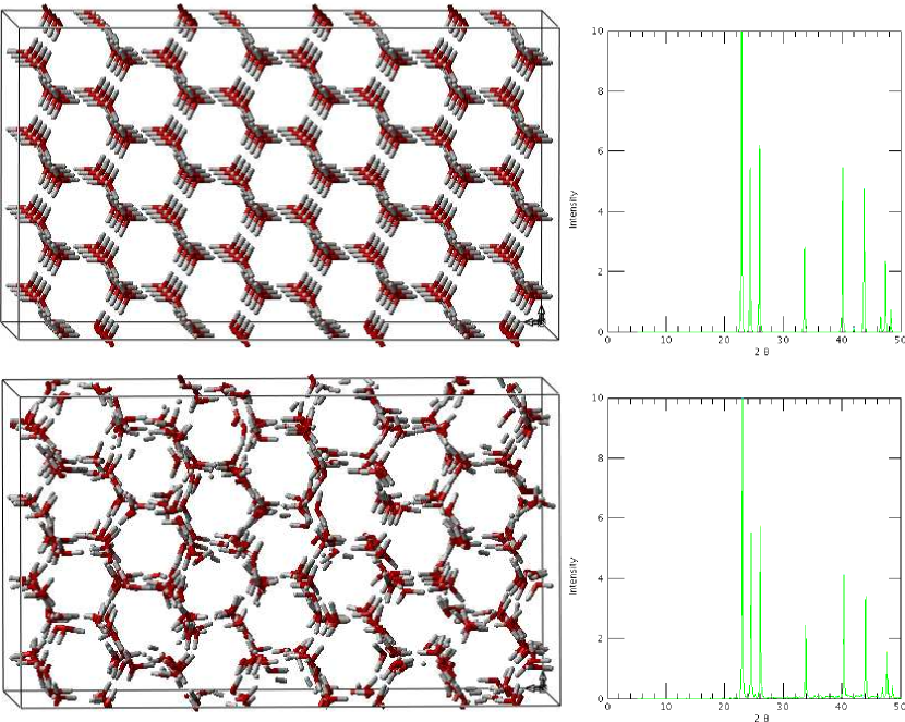
Figure 4: Structure snapshot and powder diagram of ice Ih for the ideal structure (top) and after thermalization at $T=250$ K and $P=1$ MPa (bottom)

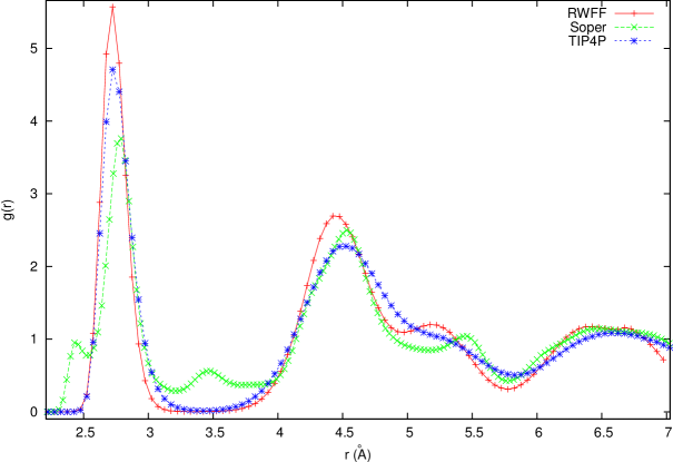
Figure 5: Oxygen radial distribution function for ice Ih after thermalization at $T=250$ K and $P=0.1$ MPa. Experimental data ($T=220$ K) from Soper (green) is compared to TIP4P (blue) and to the RWFF (red) used in this work.

V.3 Low pressure

The second batch of MD simulations has been performed slightly above atmospheric pressure at $P=1$ MPa and $T=150$ K, always following the MD procedure of Section IV. In such a thermodynamic point, all sixteen crystal structures have been studied.

Figure 6 shows the powder diagrams of the final configurations (upper part) along with the ideal structures inferred from neutron diffraction experiments (labeled as “exp”). The low pressure ices (Ic, Ih, XI) remain stable for the full simulation time of $200$ ps. The powder diagram of all high pressure ices (VII, VIII, X) loses any significant peak. The structures are unstable under low pressure and transform into amorphous ice, well reproducing the experimental results.

The “medium pressure” ices react in various ways, but to a different degree depending on their position on the phase diagram. The structures of II, III, and IX, not too far from their stability regions in the phase diagram, were stable during the entire simulations. The ices V, XII, XIII develop some distortions in the crystal structure, which are reflected by an increased background noise in their powder diagrams. The modification VI, whose stability region occurs at a higher pressure, and the metastable modification IV, collapse completely.

The dendrogram shown in Fig. 6 (lower part) has been generated by applying the clustering method to the whole set of initial and final configurations, and offers a quick summary of the whole set of behaviors described above.

The cluster can be divided in three different categories: ‘amorphous’, ‘stable with some deformation’ and ‘stable’ crystal structures (respectively red, blue and green in Fig. 6).

All amorphized structures (IV, VI, VII and VIII) form one single subcluster with a tiny distance measure ($\sim 0.01$), indicating that all of the structures are more or less identical.

All partially deformed crystal structures (V, XII and XIII) belong to a different subcluster. However, their relative distances within the dendrogram are larger than those seen within the amorphized (red) subcluster, indicating a higher differentiation among the structures. Distance between ice V and XIII is small due to the known ordered/disordered proton structure relationship. Indeed, all three powder diagrams maintain the significant peaks inherited from the original structures.

For all the stable crystal structures, the final and the initial configurations turn out to be very similar, but in the case of ice crystal couples which only differ for the proton order/disorder status (Ih/XI and III/IX), initial and final samples cannot be distinguished and belong to a single subcluster.

Simulation of ice X was not possible at low pressure due to the huge forces at the beginning of the simulation not being compensated by external pressure.

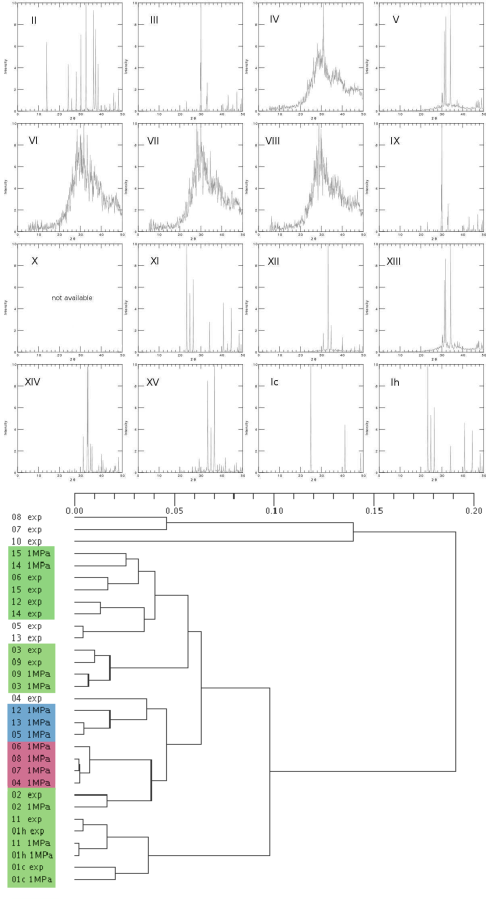
Figure 6: Simulated powder diagrams of the final crystal structures at $T=150$ K and $P=1$ MPa and their related dendrogram. Green indicates stability, blue stands for stability with some crystal distortion and red for total amorphization of the structure. MD simulation of ice X at this pressure was not possible. Ideal structures coming from diffraction experiments are also included to show the pairings with simulated crystals.

V.4 High pressure

The third batch of MD simulations was calculated at $T=150$ K and $P=1$ TPa. Also in this thermodynamic point, all sixteen crystal structures have been studied. The results are summarized in Figure 7. It should be noted that the scale used in this dendrogram is much smaller with respect to the low pressure dendrogram because more structures collapse (so becoming all quite similar) and also because we decided not to respresent the perfect theoretical structures. The high pressure polymorphs of ice, VII, VIII, and X, turn out to be stable even if some slight deformation of the crystals is observed. All of the relevant peaks are retained nonetheless. The other structures fall into two clusters. The first one contains partially amorphized crystals (ices VI, XII, XIV and XV), while the other one contains structures which became almost completely amorphous (ices Ic, Ih and XI). From Fig. 1, it is clear that all polymorphs belonging to the second cluster are stable at low pressure while, and as already observed for the low pressure simulations, the medium pressure polymorphs behave in a mixed way. The remaining ice structures, II, III, IV, V, IX and XIII, collapse completely during the simulation.

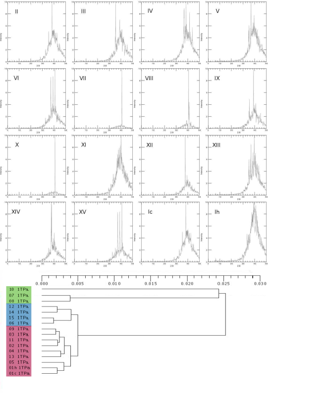
Figure 7: Simulated powder diagrams of the final crystal structures at T=$150$ K and P=$1$ TPa and the related dendrogram. Green indicates stability, blue stands for partial stability and violet total amorphization of the structure.

VI Conclusions

The present study was able to show that, within a proper force field parameterization, classical Molecular Dynamics can be successfully used to simulate the temperature and pressure dependence of static properties of ice crystals, such as structure, proton order-disorder relations and phase stability.

The success is linked to the use of the RWFF potential which, at the moment, appears to be one of the most powerful potentials for the description of water properties over an extended range of thermodynamic conditions, as well as in different complex systems such as, for example, hydrated acid polymers.

The success of the approach is shown through the use of a computational crystallography protocol, which is based on MD simulations, powder diffraction diagram determination and cluster analysis.

The proposed protocol appears to be powerful, stable and well suited for automated crystal structures determination.

References

- (1) E.A. Zheligovskaya and G. Malenkov, “Crystalline water ices” Russian Chemical Reviews 75, 57 (2006).
- (2) B. Guillot, “A reappraisal of what we have learnt during three decades of computer simulations on water” Journal of Molecular Liquids 101, 219–260 (2002).
- (3) E. Sanz, C. Vega, J.L.F. Abascal, and L.G. MacDowell, “Phase diagram of water from computer simulation” Phys. Review Letters 92, 255701 (2004).
- (4) A. Baranyai, A. Bartok, and A. Chialvo, “Computer simulations of the 13 crystalline phases of ice” J. Chem. Phys. 123, 054502 (2005).
- (5) E.A. Zheligovskaya, “Molecular dynamics study of crystalline water ices” J. of Struct. Chem. 49, 459 (2008).
- (6) V.I. Poltev, T.I. Grokhlina, and G.G. Malenkov, “Hydration of nucleic acid bases studied using novel atom-atom potential functions” J. Biomol. Struct. Dyn. 2, 413 (1984).
- (7) V. Buch, R. Martonak, and M. Parrinello, “A new molecular-dynamics based approach for molecular crystal structure search” J. Chem. Phys. 123, 051108 (2005).
- (8) D. W. M. Hofmann, L. N. Kuleshova, and B. D’Aguanno, “A new reactive potential for the molecular dynamics simulation of liquid water” Chem. Phys. Letters 448, 138 (2007).
- (9) D. W. M. Hofmann, L. N. Kuleshova, and B. D’Aguanno, “Molecular dynamics simulation of hydrated nafion with a reactive force field for water” J. Mol. Model. 14, 225 (2008).
- (10) D. W. M. Hofmann, L. N. Kuleshova, and B. D’Aguanno, “Theoretical simulations of proton conductivity: Basic principles for improving the proton conductor” J.Power Sources 195, 7743–7750 (2010).
- (11) M. Chaplin, “http://www.btinternet.com/martin.chaplin/ice.html” (10 2010).
- (12) G. Malenkov, “Liquid water and ices: understanding the structure and physical properties” J.Phys. Condens. Matter 21, 1 (2009).
- (13) M.A.Carignano, P.B. Shepson, and I. Szleifer, “Molecular dynamics simulations of ice growth from supercooled water” Molecular Physics 103, 2957 (2005).
- (14) E. Moore and V. Molinero, “Growing correlation length in supercooled water” J. Chem. Phys. 130, 244505 (2009).
- (15) E. Moore, E. de la Llave, D. Scherlis, K.Welke, and V. Molinero, “Freezing, melting and structure of ice in hydrophilic nanopore” Phys. Chem. Chem. Phys 12, 4124 (2010).
- (16) D. W. M. Hofmann and L. N. Kuleshova, “New similarity index for crystal structure determination from x-ray powder diagrams” J. Appl. Cryst. 38, 861 (2005).
- (17) D. W. M. Hofmann, L. N. Kuleshova, F. Hofmann, and B. D’Aguanno, “Cluster analysis and completeness of crystal structure generation” Chem. Phys. Letters 475, 149 (2009).
- (18) D. W. M. Hofmann and L. N. Kuleshova, “A method for automated determination of the crystal structure from x-ray powder diffraction data” Crystallography Reports 51, 452 (2006).
- (19) D. W. M. Hofmann and L. N. Kuleshova, Data Mining in crystallography (Springer Verlag, 2010).
- (20) C. Lee, D. Vanderbilt, K. Laasonen and R. Car, and M.Parrinello, “Ab initio studies on high pressure phases of ice” Phys. Rev. Lett. 69, 462 (1992).
- (21) C. Lobban, J.L. Finney, and W.F. Kuhs, “The structure of a new phase of ice” Nature 391, 268–270 (1998).
- (22) “http://www.fiz-karlsruhe.de/icsd.html” .
- (23) D. W. M. Hofmann, “http://www.flexcryst.com/home.pdf” (10 2010).
- (24) “W. Smith, CCLRC, Daresbury Laboratory, England,” .
- (25) J.D. Bernal and R.H. Fowler, “A theory of water and ionic solution, with particular reference to hydrogen and hydroxyl ions” J. Chem Phys. 1, 515 (1933).
- (26) L. Verlet, “Computer “experiments” on classical fluids. I. thermodynamical properties of Lennard-Jones molecules” Phys. Rev. 159, 98 (1967).
- (27) A.K. Soper,“The radial distribution functions of water and ice from 220 to 673 K and at pressures up to 400 MPa” Chemical Physics 258, 121 (2000).
- (28) C. Vega, C. McBride, E. Sanz and J.L.F. Abascal,“Radial distribution functions and densities for the SPC/E, TIP4P and TIP5P models for liquid water and ices Ih, Ic, …” Phys. Chem. Chem. Phys. 7, 1450 (2005).
- (29) M. Martin-Conde, L.G. MacDowell and C. Vega,“Computer simulation of two new solid phases of water: Ice XIII and ice XIV” J. Chem. Phys. 125, 116101 (2006).
- (30) W.F. Kuhs and M.S. Lehmann,“The Structure of Ice Ih by Neutron Diffraction” J. Phys. Chem. 87, 4312 (1983).
- (31) M.D. Morse, S.A. Rice,“A test of the accuracy of an effective pair potential for liquid water” J. Chem. Phys. 74, 6514 (1981).