Fermion Energies in the Background of a Cosmic String

Abstract

We provide a thorough exposition, including technical and numerical details, of previously published results on the quantum stabilization of cosmic strings. Stabilization occurs through the coupling to a heavy fermion doublet in a reduced version of the standard model. We combine the vacuum polarization energy of fermion zero–point fluctuations and the binding energy of occupied energy levels, which are of the same order in a semi–classical expansion. Populating these bound states assigns a charge to the string. We show that strings carrying fermion charge become stable if the electro–weak bosons are coupled to a fermion that is less than twice as heavy as the top quark. The vacuum remains stable in our model, because neutral strings are not energetically favored. These findings suggests that extraordinarily large fermion masses or unrealistic couplings are not required to bind a cosmic string in the standard model.

I Introduction

It is well–known that the electroweak standard model and many of its extensions have the potential to support string–like configurations that are the particle physics analogs of vortices or magnetic flux tubes in condensed matter physics. Such objects are usually called cosmic strings to distinguish them from the fundamental variables in string theory, and also to indicate that they typically stretch over cosmic length scales.

The topology of string–like configurations is described by the first homotopy group $\Pi_{1}(\mathscr{M})$, where $\mathscr{M}$ is the manifold of vacuum field configurations far away from the string. In typical electroweak–like models, a Higgs condensate breaks an initial gauge group $G$ down to some subgroup $H$, so that $\mathscr{M}\simeq G/H$. Topologically stable strings are therefore ruled out in the electroweak standard model $SU(2)\times U(1)\to U(1)$ because $G/H$ is simply connected. Nevertheless, one could envision a GUT and/or supersymmetric extension in which a simply connected group $G$ breaks down to the electroweak $SU(2)\times U(1)$ at a much higher scale, so that $\Pi_{1}(G/(SU(2)\times U(1)))$ is nontrivial. Since such GUT strings would have enormous energy densities, they could be seen by direct observation using gravitational lensing Kibble:1976sj ; Hindmarsh:1994re or by signatures in the cosmic microwave background Vilenkin:1994 . Moreover, a network of such strings is a candidate for the dark energy required to explain the recently observed cosmic acceleration Perlmutter:1998np ; Riess:1998cb .

The absence of topological stability does not imply that electroweak strings (or $Z$–strings Vachaspati:1992fi ; Achucarro:1999it ; Nambu:1977ag ) are unstable or irrelevant for particle physics. While their direct gravitational effects are negligible, $Z$–strings can still be relevant for cosmology at a sub–dominant level Copeland:2009ga ; Achucarro:2008fn . Their most interesting consequences originate, however, from their coupling to the standard model fields. $Z$–strings provide a source for primordial magnetic fields Nambu:1977ag and they also offer a scenario for baryogenesis with a second order phase transition Brandenberger:1992ys ; Brandenberger:1994bx . In contrast, a strong first order transition as required by the usual bubble nucleation scenario is unlikely in the electroweak standard model EWPhase , without non-standard additions such as supersymmetry or higher–dimensional operators Grojean:2004xa . Because the core of the $Z$–string is characterized by a suppressed Higgs condensate, it allows for both the copious baryon number violation and the out–of equilibrium regions required by the Sakharov conditions, without relying on a first order phase transition.

However, these interesting effects are only viable if $Z$–strings are energetically stabilized by their coupling to the remaining quantum fields. The most important contributions are expected to come from (heavy) fermions, since their quantum energy dominates in the limit $N_{C}\to\infty$, where $N_{C}$ is the number of QCD colors or other internal degrees of freedom. The Dirac spectrum in typical string backgrounds is deformed to contain either an exact or near zero mode, so that fermions can substantially lower their energy by binding to the string. This binding effect can overcome the classical energy required to form the string background. However, the remaining spectrum of modes is also deformed and for consistency its contribution (the vacuum polarization energy) must be taken into account as well. Heavier fermions are expected to provide more binding since the energy gain per fermion charge is higher; a similar conclusion can also be obtained from decoupling arguments D'Hoker:1984ph ; D'Hoker:1984pc . Dynamical stability of $Z$–strings in the full standard model also would suggest that they are presently observable.

A number of previous studies have investigated quantum properties of string configurations. Naculich Naculich:1995cb has shown that in the limit of weak coupling, fermion fluctuations destabilize the string. The quantum properties of $Z$–strings have also been connected to non–perturbative anomalies Klinkhamer:2003hz . The emergence or absence of exact neutrino zero modes in a $Z$–string background and the possible consequences for the string topology were investigated in Stojkovic . A first attempt at a full calculation of the fermionic quantum corrections to the $Z$–string energy was carried out in ref. Groves:1999ks . Those authors were only able to compare the energies of two string configurations, rather than comparing a single string configuration to the vacuum because of limitations arising from the non–trivial behavior at spatial infinity which we discuss below. The fermionic vacuum polarization energy of the Abelian Nielsen–Olesen vortex Nielsen:1973cs has been estimated in ref. Bordag:2003at with regularization limited to the subtraction of the divergences in the heat–kernel expansion. Quantum energies of bosonic fluctuations in string backgrounds were calculated in ref. Baacke:2008sq . Finally, the dynamical fields coupled to the string can also result in (Abelian or non–Abelian) currents running along the string’s core. The time evolution of such structured strings was studied in ref. Lilley:2010av , where the current was induced by the coupling to an extra scalar field.

We have previously pursued the idea of stabilizing cosmic strings by populating fermionic bound states in a $2+1$ dimensional model Graham:2006qt . Many such bound states emerge including, in some configurations, an exact zero–mode Naculich:1995cb . Nonetheless, stable configurations were only obtained for extreme values of the model parameters. In $3+1$ dimensions, stability is potentially easier to achieve because quantization of the momentum parallel to the symmetry axis supplies an additional multiplicity of bound states.

In this paper, we will employ the phase–shift approach, or spectral method, to compute the complete $\mathcal{O}(\hbar)$ fermionic contribution to the string energy from first principles. This is not a simple task, since the string has a vortex structure that introduces non–trivial field winding at spatial infinity. The standard spectral methods are thus not directly applicable since scattering theory off the string is ill–defined. More precisely, the Born expansion to the vacuum polarization energy, which in the phase shift approach is identified with the Feynman series, does not exist for the string background in its standard formulation. Recently we have shown how to overcome these problems by choosing a particular set of gauges Weigel:2009wi ; Weigel:2010pf . Numerical results of the full calculation of the string’s quantum energy were first reported in ref. Weigel:2010zk . Here we will present the technical details of our calculation along with improved numerical data and a discussion of possible consequences of our finding.

This paper is organized as follows: In the next section we describe our model and the string configuration. We then discuss the fermion Hamiltonian of our model and, in particular, how a local gauge transformation can be used to solve the technical problem of long–ranged gauge potentials in the string background. We also present the grand spin decomposition of the scattering problem. Section IV gives a detailed account of our method for computing the fermion quantum energy, which is based on the spectral approach Graham:2009zz and the interface formalism Graham:2001dy . The individual contributions to the string’s quantum energy are described in separate subsections, while some (lengthy) numerical details are deferred to appendices A, B, and C. The omission of boson fluctuations causes the model not to be asymptotically free which then introduces an unphysical Landau pole. In appendix D we verify that our results for the vacuum polarization energy are not affected by this artifact. In section V, we explain our variational search for a stable string configuration. To occupy fermion levels in the string background, we introduce a quantity similar to the chemical potential in statistical mechanics, which allows us to compute the total binding energy of the string as a function of the prescribed fermion charge of the string.

Our numerical results are presented in detail within section VI. We show the parameter dependence of the individual contributions to the string’s quantum energy. The stable configuration is discussed in more detail and it is shown that for the most stable configuration the gauge field contribution is negligible compared to the deformation of the Higgs field. Stabilization occurs for otherwise realistic parameters if the Yukawa coupling is increased by about 70% from the value for the top quark. Since we keep all other parameters as suggested by the standard model, this corresponds to a fermion mass of about $300\,\mathrm{GeV}$. We close in section VII with a brief summary of our results, a discussion of its implication for the electroweak standard model and an outlook on possible directions for future work.

We have published some of the results earlier Weigel:2010zk and therefore focus on the technical aspects of the calculation here.

II The model

We consider a left–handed $SU(2)$ gauge theory in which a fermion doublet $\Psi=\begin{pmatrix}\Psi_{t}\cr\Psi_{b}\end{pmatrix}$ is coupled to a triplet gauge field $W_{\mu}=\frac{1}{2}\begin{pmatrix}W^{0}_{\mu}&\sqrt{2}W^{+}_{\mu}\\[5.69054pt] \sqrt{2}W^{-}_{\mu}&-W^{0}_{\mu}\end{pmatrix}$ and a Higgs doublet $\phi=\begin{pmatrix}\phi_{+}\cr\phi_{0}\end{pmatrix}$. Both components, $\Psi_{t}$ and $\Psi_{b}$, are Dirac four–spinors. This model is intended to represent the electroweak interactions, where we introduce some technical modifications to simplify the analysis:

1. we set the Weinberg angle to zero so that electromagnetism decouples and the gauge bosons become degenerate in mass;

2. we neglect QCD interactions, although the color degeneracy, $N_{C}=3$, is included in the quantum energy arising from the fermions;

3. we only consider a single fermion doublet and neglect inter–species (CKM) mixing and mass splitting within the doublet.

With these adjustments, the bosonic part of our model is described by the Lagrangian

$$\mathcal{L}_{\phi,W}=-\frac{1}{2}\mbox{tr}\left(G^{\mu\nu}G_{\mu\nu}\right)+\frac{1}{2}\mbox{tr}\left(D^{\mu}\Phi\right)^{{\dagger}}D_{\mu}\Phi-\frac{\lambda}{2}\mbox{tr}\left(\Phi^{{\dagger}}\Phi-v^{2}\right)^{2}\,,$$ (1)

where the Higgs doublet is written using the usual matrix representation

$$\Phi=\begin{pmatrix}\phi_{0}^{*}&\phi_{+}\cr-\phi_{+}^{*}&\phi_{0}\end{pmatrix}\,.$$

The gauge coupling constant $g$ enters through the covariant derivative $D_{\mu}=\partial_{\mu}-i\,gW_{\mu}$, and the $SU(2)$ field strength tensor is

$$G_{\mu\nu}=\partial_{\mu}\,W_{\nu}-\partial_{\nu}W_{\mu}-i\,g\,[\,W_{\mu}\,,\,W_{\nu}\,]\,.$$ (2)

We treat the bosonic fields as a classical background, ignoring the effects of bosonic fluctuations. This approach can be justified formally by the limit of a large number of colors $N_{C}\to\infty$, even though no QCD interactions are included: Since the quarks carry a color quantum number in the fundamental representation of the color group $SU(N_{C})$, their contribution to the quantum energy is enhanced by a factor $N_{C}$ as compared to the bosonic quantum contribution. Hence we compute the leading quantum corrections to the classical background energy from the fermion Lagrangian

$$\mathcal{L}_{\Psi}=i\overline{\Psi}\left(P_{L}D\hskip-6.00006pt/+P_{R}\partial\hskip-6.00006pt/\right)\Psi-f\,\overline{\Psi}\left(\Phi P_{R}+\Phi^{\dagger}P_{L}\right)\Psi\,.$$ (3)

Here, $P_{R,L}=\frac{1}{2}\left(1\pm\gamma_{5}\right)$ are projection operators on left/right–handed components, respectively, and the strength of the Higgs-fermion interaction is parameterized by the Yukawa coupling $f$, which gives rise to the fermion mass, $m=fv$, once the Higgs acquires a vacuum expectation value ($vev$) $v$, where $\langle{\rm det}(\Phi)\rangle=v^{2}\neq 0$. All other masses in this model are also a result of the symmetry breaking Higgs condensate, viz. the gauge boson mass $M_{W}=gv/\sqrt{2}$ and the Higgs mass $m_{H}=2v\,\sqrt{\lambda}$. This similarity with the standard model of particle physics suggests the model parameters

$$g=0.72\,,\quad v=177\,{\rm GeV}\,,\quad m_{\rm H}=140\,{\rm GeV}\,,\quad f=0.99\,,$$ (4)

by taking the fermion doublet to have the mass of the top quark. Finally, the counterterm Lagrangian necessary to renormalize the quantum energy will be listed with the computational details in eq. (44) below.

As mentioned earlier, we are particularly interested in the $Z$–string background configuration. If we consider a single straight (infinitely extended) string along the $z$–axis, the corresponding boson fields depend only on the planar polar coordinates, i.e. the distance $\rho$ from the symmetry axis and the corresponding azimuthal angle $\varphi$. In Weyl gauge $W_{0}=0$, we have

$$\mathbf{W} = n\,{\rm sin}(\xi_{1})\,\frac{f_{G}(\rho)}{\rho}\,\widehat{\mbox{\boldmath$\varphi$\unboldmath}}\,\begin{pmatrix}{\rm sin}(\xi_{1})&i\,{\rm cos}(\xi_{1})\,{\rm e}^{-in\varphi}\\[5.69054pt] -i\,{\rm cos}(\xi_{1})\,{\rm e}^{in\varphi}&-{\rm sin}(\xi_{1})\end{pmatrix}$$ (5)

$$\Phi = vf_{H}(\rho)\begin{pmatrix}{\rm sin}(\xi_{1})\,{\rm e}^{-in\varphi}&-i\,{\rm cos}(\xi_{1})\\[5.69054pt] -i\,{\rm cos}(\xi_{1})&{\rm sin}(\xi_{1})\,{\rm e}^{in\varphi}\end{pmatrix}\,.$$ (6)

The $Z$–boson component $Z_{\mu}\equiv W_{\mu}^{3}$ of this configuration has the familiar shape of an Abelian Nielsen–Olesen string of winding number $n$, although the entire non–Abelian configuration is smoothly deformable into the vacuum and thus not stable for any topological reason. We have left the analog of winding number $n$ general, although we will only consider $n=1$ in our numerical treatment below. The additional variational parameter $\xi_{1}\in[0,\nicefrac{{\pi}}{{2}}]$ was introduced to include a non–trivial gauge field in the string background; the same parameter also determines the orientation of the Higgs field on the chiral circle. Then the classical energy per unit length of the string is a functional of the profile functions $f_{G}(\rho)$ and $f_{H}(\rho)$,

$$\frac{E_{\rm cl}}{m^{2}}=2\pi\int_{0}^{\infty}\rho\,d\rho\,\left\{n^{2}\sin^{2}\xi_{1}\,\biggl{[}\frac{2}{g^{2}}\left(\frac{f_{G}^{\prime}}{\rho}\right)^{2}+\frac{f_{H}^{2}}{f^{2}\rho^{2}}\,\left(1-f_{G}\right)^{2}\biggr{]}+\frac{f_{H}^{\prime 2}}{f^{2}}+\frac{\mu_{h}^{2}}{4f^{2}}\left(1-f_{H}^{2}\right)^{2}\right\}\,,$$ (7)

where the radial integration variable is related to the physical radius by $\rho_{\rm phys}=\rho/m$ and $\mu_{H}\equiv m_{H}/m$. The radial functions $f_{G}(\rho)$ and $f_{H}(\rho)$ in the string configuration, eqs. (5) and (6) approach unity at large distances and vanish at the string core $\rho=0$. Typically, they will have similar shapes to the familiar Nielsen–Olesen string, with both $\mathbf{W}$ and $\Phi$ going as $\mathscr{O}(\rho)$ at $\rho\to 0$ to avoid ambiguities from an undefined azimuthal angle $\varphi$. We choose a convenient form,

$$f_{H}(\rho)=1-\exp\left[-\frac{\rho}{w_{H}}\right]\quad\mbox{and}\quad f_{G}(\rho)=1-\exp\left[-\left(\frac{\rho}{w_{G}}\right)^{2}\right]\,$$ (8)

with two width parameters, $w_{H}$ and $w_{G}$, which we also measure in inverse multiples of the fermion mass $m$. Together with the angle $\xi_{1}$ describing the gauge field admixture in the string, we thus have three variational ansatz parameters, $(w_{H},w_{G},\xi_{1})$, in addition to the model parameters $v$ (which sets the overall scale) and the three couplings $f,g$ and $\lambda$, that are discussed above.

To assess the quality of the variational ansatz, eq. (8) we see how well it is capable of fitting the Nielsen–Olesen profiles which minimize the classical energy, eq. (7) for $\xi_{1}=\nicefrac{{\pi}}{{2}}$.

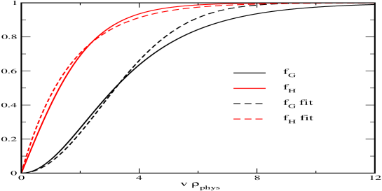
Figure 1: (Color online) Comparison between the Nielsen–Olesen profiles (full lines) and a fit using the variational ansatz of eq. (8) (dashed lines). The variational parameters are $w_{H}=1.64f$ and $w_{G}=3.85f$.

As seen from figure 1 there is a minor discrepancy at large distances for the gauge field profile $f_{G}$ due to the Gaußian decaying faster than any exponential function. This discrepancy affects the result for the classical energy in a negligible manner. For fixed $\xi_{1}=\nicefrac{{\pi}}{{2}}$ the true minimum is at $7.56v^{2}$ while the variational profiles yield $7.72v^{2}$.

III Dirac Hamiltonian

The fermionic quantum corrections to the string background are computed in several steps. First, we extract the Dirac Hamiltonian associated with the Lagrangian eq. (3) and observe that the ansätze, eqs. (5) and (6), do not depend on the $z$–coordinate (along the string symmetry axis). Hence this coordinate does not appear explicitly in the Hamiltonian and the $z$–dependence of the corresponding wave functions is simply $e^{-ip_{z}z}$. To compute the vacuum energy with such a trivial coordinate, we use the interface formalism Graham:2001dy , which gives the quantum energy per unit length in terms of the two–dimensional spectrum in the plane perpendicular to the string. This formulation accounts for the integration over the longitudinal momentum $p_{z}$ using sum rules for the scattering data Graham:2001iv ; Puff:1975zz to cope with the associated ultra–violet divergences. It then remains to solve the scattering problem for the Hamiltonian in the plane perpendicular to the string.

Although we are thus left with a seemingly well–defined two–dimensional Dirac problem, the spectral method cannot be readily applied to compute the vacuum energy, because the long range of the string gauge field prevents us from setting up a well–defined scattering problem. There are two ways to circumvent this problem: As motivated by the study of quantum effects for QED flux tubes Graham:2004jb , a return string was introduced in ref. Weigel:2009wi to unwind the gauge field at a large distance from the string core. The assumption was that the energy of the return string is small when the unwinding is done smoothly enough and, in particular, that the associated energy density can be well separated from the proper string core contribution. Although these assumptions could be verified, the necessity to repeat the (expensive) calculation of the vacuum energy with varying return string positions to identify the core contribution made the return string method inefficient for actual calculations.

An easier method was devised in ref. Weigel:2010pf . It is based on the simple observation that the Dirac spectrum is gauge invariant, i.e. a local isospin rotation can be used to unwind the string gauge field at spatial infinity at the price of strong singularities in the origin (singular gauge), or to make the gauge field regular at the origin at the price of long–ranged fields at spatial infinity (regular gauge). The solution is to combine the good features of both gauges by means of a local gauge rotation that looks singular for large distances and regular for small distances. Thus, we make a local gauge rotation on the Dirac Hamiltonian $H\to U^{\dagger}\,H\,U$ with

$$U=P_{L}{\rm exp}\,\Big{(}i\,\xi(\rho)\,\mathbf{n}\cdot\mbox{\boldmath$\tau$\unboldmath}\Big{)}+P_{R}\qquad{\rm with}\qquad\mathbf{n}=\begin{pmatrix}{\rm cos}(n\varphi)\cr-{\rm sin}(n\varphi)\cr 0\end{pmatrix}\,.$$ (9)

Here $\xi(\rho)$ is an arbitrary radial function that defines a set of gauge transformations. Note that $\xi=0$ gives back the original regular Hamiltonian, while $\xi=\xi_{1}$ together with $f_{H}\equiv f_{G}\equiv 1$ at large distances yields the return string configuration considered in ref. Weigel:2009wi . Thus the interpolation between regular and singular behavior is accomplished by the boundary conditions $\xi(0)=0$ and $\xi(\infty)=\xi_{1}$. The transformed Dirac Hamiltonian becomes

$$H = -i\begin{pmatrix}0&\mbox{\boldmath$\sigma$\unboldmath}\cdot\widehat{\mbox{\boldmath$\rho$\unboldmath}}\cr\mbox{\boldmath$\sigma$\unboldmath}\cdot\widehat{\mbox{\boldmath$\rho$\unboldmath}}&0\end{pmatrix}\partial_{\rho}-\frac{i}{\rho}\begin{pmatrix}0&\mbox{\boldmath$\sigma$\unboldmath}\cdot\widehat{\mbox{\boldmath$\varphi$\unboldmath}}\cr\mbox{\boldmath$\sigma$\unboldmath}\cdot\widehat{\mbox{\boldmath$\varphi$\unboldmath}}&0\end{pmatrix}\partial_{\varphi}+H_{\rm int}\,,$$

$$H_{\rm int} = mf_{H}\left[{\rm cos}(\Delta)\begin{pmatrix}\mbox{{\sf 1}\mbox{}\rule{0.39993pt}{6.6736pt}\mbox{\hskip 1.00006pt}}&0\cr 0&-\mbox{{\sf 1}\mbox{}\rule{0.39993pt}{6.6736pt}\mbox{\hskip 1.00006pt}}\end{pmatrix}+i\,{\rm sin}(\Delta)\begin{pmatrix}0&\mbox{{\sf 1}\mbox{}\rule{0.39993pt}{6.6736pt}\mbox{\hskip 1.00006pt}}\cr-\mbox{{\sf 1}\mbox{}\rule{0.39993pt}{6.6736pt}\mbox{\hskip 1.00006pt}}&0\end{pmatrix}\mathbf{n}\cdot\mbox{\boldmath$\tau$\unboldmath}\right]+\frac{1}{2}\frac{\partial\xi}{\partial\rho}\begin{pmatrix}-\mbox{\boldmath$\sigma$\unboldmath}\cdot\widehat{\mbox{\boldmath$\rho$\unboldmath}}&\mbox{\boldmath$\sigma$\unboldmath}\cdot\widehat{\mbox{\boldmath$\rho$\unboldmath}}\cr\mbox{\boldmath$\sigma$\unboldmath}\cdot\widehat{\mbox{\boldmath$\rho$\unboldmath}}&-\mbox{\boldmath$\sigma$\unboldmath}\cdot\widehat{\mbox{\boldmath$\rho$\unboldmath}}\end{pmatrix}\mathbf{n}\cdot\mbox{\boldmath$\tau$\unboldmath}$$ (10)

$$+\frac{n}{2\rho}\,\begin{pmatrix}-\mbox{\boldmath$\sigma$\unboldmath}\cdot\widehat{\mbox{\boldmath$\varphi$\unboldmath}}&\mbox{\boldmath$\sigma$\unboldmath}\cdot\widehat{\mbox{\boldmath$\varphi$\unboldmath}}\cr\mbox{\boldmath$\sigma$\unboldmath}\cdot\widehat{\mbox{\boldmath$\varphi$\unboldmath}}&-\mbox{\boldmath$\sigma$\unboldmath}\cdot\widehat{\mbox{\boldmath$\varphi$\unboldmath}}\end{pmatrix}\Big{[}f_{G}\,{\rm sin}(\Delta)I_{G}(\Delta)+(f_{G}-1)\,{\rm sin}(\xi)I_{G}(-\xi)\Big{]}\,.$$

The new gauge function $\xi(\rho)$ is hidden in the difference $\Delta(\rho)\equiv\xi_{1}-\xi(\rho)$ which appears both explicitly and as the argument of the space–dependent weak isospin matrix

$$I_{G}(x)=\begin{pmatrix}-{\rm sin}(x)&-i\,{\rm cos}(x)\,{\rm e}^{in\varphi}\\[5.69054pt] i\,{\rm cos}(x)\,{\rm e}^{-in\varphi}&{\rm sin}(x)\end{pmatrix}\,.$$ (11)

All explicit matrices in eq. (10) act in spinor space. Together with the boundary conditions for the string profiles $f_{G}$ and $f_{H}$, eq. (10) defines a well–behaved scattering problem for which a scattering matrix and, more generally, a Jost function can be straightforwardly computed. Moreover, the Born series to these scattering data can be constructed simply by iterating $H_{\rm int}$.

We will renormalize the calculation by subtracting orders of the Born series and adding these contributions back as the corresponding Feynman diagrams. It should be mentioned that although the Jost function is gauge invariant, neither the Born series nor the individual Feynman diagrams associated with eq. (10) is gauge invariant, and so the Born subtracted phase shifts or Jost functions will also depend on the gauge. That is, these quantities are functionals of $\xi(\rho)$. However, the gauge–dependent terms subtracted from the phase shifts correspond exactly to the gauge–dependent finite parts in the Feynman diagrams, while the counterterms, which parameterize the ultraviolet singularities, are gauge–independent. The net effect is that individual pieces of the spectral approach to the vacuum energy will be gauge–dependent, but the combined expression is not.

The formulation in eq. (10) describes the physical string without the need to introduce artificial return strings to unwind the topology. In particular, the (tedious) separation of the return string contribution from the bound state spectrum of the physical string is no longer required. Moreover, the gauge function $\xi(\rho)$ can be taken to have support at a moderate distance, so that there is no need for non–trivial fields at very large radii and, as a consequence, the need for extremely large angular momenta is avoided.

To solve the scattering problem for the Hamiltonian, eq. (10), in two space dimensions, we first introduce grand–spin states to take care of the angular dependence. For a fixed angular momentum $\ell$, there are four grand–spin states, characterized by the quantum numbers $\pm\nicefrac{{1}}{{2}}$ for spin $S$ and isospin $I$,

$$\begin{array}[]{ll}\langle\varphi;SI|\ell++\rangle={\rm e}^{i(\ell+n)\varphi}\,\begin{pmatrix}1\cr 0\end{pmatrix}_{S}\otimes\begin{pmatrix}1\cr 0\end{pmatrix}_{I}&\qquad\langle\varphi;SI|\ell+-\rangle=-i\,{\rm e}^{i\ell\varphi}\,\begin{pmatrix}1\cr 0\end{pmatrix}_{S}\otimes\begin{pmatrix}0\cr 1\end{pmatrix}_{I}\cr\cr\langle\varphi;SI|\ell-+\rangle=i\,{\rm e}^{i(\ell+n+1)\varphi}\,\begin{pmatrix}0\cr 1\end{pmatrix}_{S}\otimes\begin{pmatrix}1\cr 0\end{pmatrix}_{I}&\qquad\langle\varphi;SI|\ell--\rangle={\rm e}^{i(\ell+1)\varphi}\,\begin{pmatrix}0\cr 1\end{pmatrix}_{S}\otimes\begin{pmatrix}0\cr 1\end{pmatrix}_{I}\,.\end{array}$$ (12)

The angular dependence is thus separated from the radial dependence by the ansatz

$$\Psi_{\ell}(\rho,\varphi)=\sum_{s,j=\pm\nicefrac{{1}}{{2}}}\Big{(}\langle\rho\,|\,\langle\,\varphi\,;\,S\,I\,|\Big{)}\,|\epsilon\,\ell\,s\,j\,\rangle\,.$$ (13)

For each value of the angular momentum $\ell$, this decomposition turns the Dirac equation

$$H\Psi=\epsilon\Psi\,,$$ (14)

with the Hamiltonian given in eq. (10), into a $8\times 8$ system of ordinary first order differential equation for the radial functions in the spinor states

$$\begin{array}[]{ll}\langle\rho|\epsilon\,\ell++\rangle=\begin{pmatrix}f_{1}(\rho)|\ell++\rangle\cr g_{1}(\rho)|\ell-+\rangle\end{pmatrix}&\qquad\langle\rho|\epsilon\,\ell+-\rangle=\begin{pmatrix}f_{2}(\rho)|\ell+-\rangle\cr g_{2}(\rho)|\ell--\rangle\end{pmatrix}\cr\cr\langle\rho|\epsilon\,\ell-+\rangle=\begin{pmatrix}f_{3}(\rho)|\ell-+\rangle\cr g_{3}(\rho)|\ell++\rangle\end{pmatrix}&\qquad\langle\rho|\epsilon\,\ell--\rangle=\begin{pmatrix}f_{4}(\rho)|\ell--\rangle\cr g_{4}(\rho)|\ell+-\rangle\end{pmatrix}\,,\end{array}$$ (15)

where we have suppressed the energy label ($\epsilon$) on the radial functions. It is convenient to combine these eight functions in a vector notation

$$\vec{f}=\begin{pmatrix}f_{1}(\rho)\cr f_{2}(\rho)\cr f_{3}(\rho)\cr f_{4}(\rho)\end{pmatrix}\qquad{\rm and}\qquad\vec{g}=\begin{pmatrix}g_{1}(\rho)\cr g_{2}(\rho)\cr g_{3}(\rho)\cr g_{4}(\rho)\end{pmatrix}\,.$$ (16)

In terms of these vectors, the static Dirac equation in each angular momentum channel takes the form of two coupled real $4\times 4$ systems,

$$(\epsilon-m)\,\vec{f} = V_{uu}\,\vec{f}+\left(-CD_{u}+V_{ud}\right)\,\vec{g}$$

$$(\epsilon+m)\,\vec{g} = \left(CD_{d}+V_{du}\right)\,\vec{f}+V_{dd}\,\vec{g}\,.$$ (17)

The $4\times 4$ matrix $C={\rm diag}(-1,-1,+1,+1)$ is constant while $D_{u}$ and $D_{d}$ contain the radial derivative operator as well as the angular barrier terms. The coupling to the background profiles of the boson fields emerges via the matrices $V_{ij}$. Detailed expressions for $D_{u}$, $D_{d}$ and $V_{ij}$ are listed in appendix B. The ODE system eq. (17) is the basis of the spectral approach to the string problem.

For the gauge profile $\xi(\rho)$, any smooth function with $\xi(0)=0$ and $\xi(\infty)=\xi_{1}$ will do. For simplicity and to avoid possible singularities at $\rho\to 0$, we choose again a Gaußian profile

$$\xi(\rho)=\xi_{1}\,\Big{[}1-\exp\left(-\rho^{2}/w_{\xi}^{2}\right)\Big{]}$$ (18)

with a new width parameter $w_{\xi}$. As explained earlier, the scattering matrix without Born subtractions and the complete quantum energy should be independent of the choice of gauge and thus independent of the width parameter $w_{\xi}$. This has been verified numerically to a fairly high precision Weigel:2010pf .

IV Spectral method

In this section, we present the details of our approach to compute the fermion contribution to the vacuum energy of the string. To make the exposition clearer, we have moved overly complicated expressions and all technical derivations to the appendices. However, the complete method is still quite involved due to the many contributions that enter. We will continue the discussion of the variational approach for charged strings in section V and present numerical results in section VI.

The calculation of the fermion quantum energy is based on the Dirac equation (14). From the solutions to this equation we infer a number of distinct contributions to the energy of the string,

$$E_{f}=E_{\delta}+E_{\rm FD}+E_{\rm b}$$ (19)

In physical terms, these three contributions are

1. the non–perturbative vacuum polarization due to the string background, with the divergent low–order Feynman diagrams taken out by subtracting leading terms in the Born expansion. This piece also includes the bound state contribution to the fermion determinant;

2. the perturbative contribution of the low–order Feynman diagrams to the vacuum polarization energy, combined with the counterterms for proper renormalization. This compensates for the part that has been taken out of $E_{\delta}$ by means of the corresponding Born expansion;

3. the binding energy due to the single particle bound states that are explicitly occupied to give the string a fermion charge $Q$. More precisely, $E_{\rm b}=\Big{[}\sum\limits_{\rm occ~{}bs}\epsilon_{i}\Big{]}-Qm$ measures the energy of the populated levels relative to the same number of free fermions. We will describe this contribution in the next section.

Each of these pieces is separately finite; the first two terms are not gauge invariant, but their sum is, and so is $E_{\rm b}$.

In this section we focus on the renormalized vacuum polarization energy

$$E_{q}=E_{\delta}+E_{\rm FD}\,.$$ (20)

Potential ambiguities in $E_{q}$ that could originate from the ultra–violet divergences are fully removed by the identification of terms in the Born series with Feynman diagrams. The most important feature of $E_{q}$ is the possibility to impose renormalization conditions from the perturbative sector ($\overline{\rm MS}$ or on–shell), although the calculation is completely non–perturbative, including all orders in $H_{\rm int}$. We then combine $E_{q}$ with the classical energy $E_{\rm cl}$ required to form the bosonic string background. Quite generally, we expect $E_{\rm cl}+E_{q}>0$ once quantum fluctuations are included, since otherwise we would have an instability of the true vacuum to cosmic string condensation, which should obviously not happen.

In the following subsections, we will give brief accounts for each contribution to eq. (20). More details can be found in the appendices.

IV.1 Jost function and Born subtractions

The Born–subtracted vacuum polarization energy $E_{q}$ has contributions from bound and scattering states. These two contributions are combined in the Jost function for imaginary momenta Bordag:1994jz ; Graham:2009zz . To compute $E_{q}$ it is therefore sufficient to solve the scattering problem as in ref. Weigel:2009wi : For every energy $|\epsilon|>m$, the fermion system eq. (17) has eight real linear independent solutions $(\vec{f},\vec{g})$. In the case without a string background, these solutions are Bessel functions of integer order with the argument $z=k\rho$, where $k=\sqrt{\epsilon^{2}-m^{2}}\geq 0$. Instead of taking the (real) regular and singular Bessel functions $J_{\nu}(z)$ and $Y_{\nu}(z)$, respectively, we can formally let $(\vec{f},\vec{g})$ have complex coefficients and take Hankel function solutions instead. In this case, both the real and imaginary parts of $(\vec{f},\vec{g})$ are (linearly independent) solutions, or equivalently $(\vec{f},\vec{g})$ and their complex conjugates are independent solutions.

To describe the coupled channel scattering problem, it is convenient to put the four free linearly independent complex solutions for $\vec{f}$ and $\vec{g}$ onto the diagonal of two $4\times 4$ matrices

$$\mathcal{H}_{u} = \mbox{diag}\left(H^{(1)}_{\ell+n}(k\rho),H^{(1)}_{\ell}(k\rho),H^{(1)}_{\ell+n+1}(k\rho),H^{(1)}_{\ell+1}(k\rho)\right)$$ (21)

$$\mathcal{H}_{d} = \mbox{diag}\left(H^{(1)}_{\ell+n+1}(k\rho),H^{(1)}_{\ell+1}(k\rho),H^{(1)}_{\ell+n}(k\rho),H^{(1)}_{\ell}(k\rho)\right)\,,$$ (22)

which describe out–going asymptotic fields since

$$H_{\nu}^{(1)}(z)=J_{\nu}(z)+iY_{\nu}(z)\longrightarrow\sqrt{\frac{2}{\pi z}}\,{\rm e}^{i\left(z-\frac{\nu}{2}\pi-\frac{1}{2}\pi\right)}\,,$$ (23)

as $z\to\infty$. With this notation, the $j^{\rm th}$ linear independent solution is

$$(\vec{f})_{j}=\left[\mathcal{H}_{u}\right]_{j}\,,\qquad\quad(\vec{g})_{j}=\kappa\cdot\left[\mathcal{H}_{d}\right]_{j}$$

where $[\mathcal{H}]_{j}$ denotes the $j^{\rm th}$ row of the matrix $\mathcal{H}$. For convenience we omit the orbital angular momentum index $\ell$. By construction, the complex conjugate matrices, $\mathcal{H}_{u,d}^{\ast}$ describe incoming spherical waves. Furthermore, we have defined the relative weight of upper and lower Dirac components as

$$\kappa\equiv\frac{k}{\epsilon+m}=\frac{\epsilon-m}{k}\,.$$ (24)

For later analytic continuation we must ensure that the phase of the Jost function is odd for real momenta under $k\to-k$, which requires the branch cut structure of the square root be defined using either of the two expressions listed above.

To describe the coupling of the four channels in the actual scattering problem, it is convenient to put the linearly independent solutions for $\vec{f}$ and $\vec{g}$ again in the rows of a $4\times 4$ matrix, and factor out the free part to get simple Jost boundary conditions,

$$\begin{array}[]{r@{\,\,\,\,\longrightarrow\,\,\,\,}ll@{\qquad\mbox{and}\qquad}ll}(\vec{f})_{j}&&\displaystyle\left[\mathcal{F}\cdot\mathcal{H}_{u}\right]_{j}&&\displaystyle\left[\mathcal{F}^{*}\cdot\mathcal{H}^{\ast}_{u}\right]_{j}\\[8.53581pt] (\vec{g})_{j}&\kappa&\displaystyle\left[\mathcal{G}\cdot\mathcal{H}_{d}\right]_{j}&\kappa&\displaystyle\left[\mathcal{G}^{*}\cdot\mathcal{H}^{\ast}_{d}\right]_{j}\,.\end{array}$$ (25)

We substitute these ansätze into the Dirac equation, eq. (17), and find first order differential equations for the matrices $\mathcal{F}$ and $\mathcal{G}$. This is explicitly carried out in appendix B.1. The solutions to eq. (92) with the Jost boundary conditions

$$\lim_{\rho\to\infty}\mathcal{F}(\rho)=\lim_{\rho\to\infty}\mathcal{G}(\rho)=\mbox{{\sf 1}\mbox{}\rule{0.39993pt}{6.6736pt}\mbox{\hskip 1.00006pt}}$$ (26)

define Jost solutions to the initial Dirac problem via the representation in eq. (25). The physical scattering solution is the linear combination which at large distances is the superposition of incoming and outgoing free spherical waves and obeys the regularity condition at the origin. The relative weight of the incoming and outgoing waves defines the scattering matrix $\mathcal{S}$. Hence the physical scattering solution for the $\mathcal{F}$–type (upper) components reads

$$\Psi=\mathcal{F}^{\ast}\cdot\mathcal{H}_{u}^{\ast}+(\mathcal{F}\cdot\mathcal{H}_{u})\cdot\mathcal{S}.$$ (27)

The corresponding $\mathcal{G}$–type (lower) components are obtained by replacing $\mathcal{F}\to\mathcal{G}$ and $\mathcal{H}_{u}\to\kappa\mathcal{H}_{d}$. The physical scattering solution must be regular at the origin $\rho=0$. From this condition we extract the scattering matrix in one of two equivalent ways

$$\mathcal{S} = -\lim_{\rho\to 0}\,\mathcal{H}_{u}^{-1}\cdot\mathcal{F}^{-1}\cdot\mathcal{F}^{*}\cdot\mathcal{H}_{u}^{\ast}$$ (28)

$$\mathcal{S} = -\lim_{\rho\to 0}\,\mathcal{H}_{d}^{-1}\cdot\mathcal{G}^{-1}\cdot\mathcal{G}^{*}\cdot\mathcal{H}_{d}^{\ast}\,.$$ (29)

The phase convention in eq. (27) is chosen to reproduce $\mathcal{S}=\mbox{{\sf 1}\mbox{}\rule{0.39993pt}{6.6736pt}\mbox{\hskip 1.00006pt}}$ for the non–interacting case which has $\mathcal{F}^{(0)}=\mathcal{G}^{(0)}=\mbox{{\sf 1}\mbox{}\rule{0.39993pt}{6.6736pt}\mbox{\hskip 1.00006pt}}$. The equality of the two representations from the system of coupled differential equations is a good check on our numerics, as is the requirement that $\mathcal{S}$ be unitary.

It should finally be noted that all the interaction matrices eq. (95) are linear in the background profiles eq. (90), so that the ODE system for the Born approximation can simply be obtained by iteration with the ansatz

$$\mathcal{F}_{\rm Born}(\rho)=\sum_{i=0}^{\infty}\mathcal{F}^{(i)}(\rho)\qquad{\rm and}\qquad\mathcal{G}_{\rm Born}(\rho)=\sum_{i=0}^{\infty}\mathcal{G}^{(i)}(\rho)\,,$$ (30)

where the superscript denotes the order of the interaction Hamiltonian $H_{\rm int}$ in eq. (10). The zeroth order solutions are $\mathcal{F}^{(0)}(\rho)=\mathcal{G}^{(0)}(\rho)=\mbox{{\sf 1}\mbox{}\rule{0.39993pt}{6.6736pt}\mbox{\hskip 1.00006pt}}$ and all subsequent contributions are subject to the boundary conditions

$$\lim_{\rho\to\infty}\mathcal{F}^{(i)}(\rho)=\lim_{\rho\to\infty}\mathcal{G}^{(i)}(\rho)=0\,,\qquad\quad i=1,2,3\ldots$$

The explicit form of the iterated system of differential equations for the Born approximations of order $i=1$ and $i=2$ can be found in appendix B. Though the $i=3$ and $i=4$ orders also yield divergences, we do not discuss them explicitly because we employ a numerically less costly method to handle these logarithmic divergences, as described below.

IV.2 Interface formalism

The $4\times 4$ scattering matrix $\mathcal{S}$ derived in the last subsection yields the four eigenphase shifts and thus the shift in the two–dimensional density of states Graham:2002xq

$$\rho_{\ell}(k)-\rho_{\ell}^{(0)}(k)=\frac{1}{\pi}\,\sum_{c=1}^{4}\,\frac{d\delta_{\ell,c}}{dk}=\frac{i}{2\pi}\,\frac{d}{dk}\,\ln\mathrm{det}\,\mathcal{S}_{\ell}(k)\,,$$ (31)

where the sum runs over the four scattering channels for a given grand spin channel, which we label by the associated orbital angular momentum $\ell$. To turn this two–dimensional density into a three–dimensional energy (or energy per unit length of the string), we have to deal with the trivial dynamics along the string symmetry axis of the string. This is a typical application of the interface formalism developed in ref. Graham:2001dy . The modifications of the usual spectral method are simple:

1. The integration over the momentum conjugate to the coordinate of translational invariance remains finite due to sum rules for scattering data Graham:2001iv ; Puff:1975zz that are generalizations of Levinson’s theorem.

2. When integrating over momentum $k$, the density, eq. (31), must be multiplied by a kinematic factor that differs from the usual one–particle energy $\epsilon=\sqrt{m^{2}+k^{2}}$.

3. More Born subtractions are required to make the momentum integral and angular momentum sum convergent. This corresponds to the larger number of divergent Feynman diagrams in three dimensions.

Then the interface formula for the vacuum polarization energy per unit length of the string is

$$E_{\delta}^{(N)} = \frac{1}{4\pi}\sum_{\ell=-n}^{\infty}\Bigg{\{}D_{\ell}\int_{0}^{\infty}\frac{dk}{\pi}\left[(k^{2}+m^{2}){\rm ln}\left(\frac{k^{2}+m^{2}}{\mu^{2}}\right)-k^{2}\right]\,\frac{d}{dk}\left[\delta_{\ell}(k)\right]_{N}$$ (33)

$$\hskip 56.9055pt+\sum_{j}\left[\left(\epsilon_{j,\ell}\right)^{2}{\rm ln}\frac{\left(\epsilon_{j,\ell}\right)^{2}}{\mu^{2}}-\left(\epsilon_{j,\ell}\right)^{2}+m^{2}\right]\Bigg{\}}\,,$$

where the notation $[\cdots]_{N}$ refers to the quantity in the brackets with its first $N$ terms of the Born series subtracted. For the string problem in three space dimensions, we need $N\geq 4$ to ensure convergence of the momentum integral although, as described below, we will use a different subtraction in place of the $N=3$ and $N=4$ cases. Here, $\epsilon_{j,\ell}$ gives the energy of the $j^{\rm th}$ bound state in the angular momentum channel $\ell$, and $D_{\ell}$ is the degeneracy in that channel. For the string background, we have

$$D_{\ell}=\begin{cases}1\,,\quad&\ell=-n\cr 2\,,\quad&\ell>-n\,,\end{cases}$$ (34)

where $n=1$ is the Higgs winding number introduced in the string configuration of eqs. (5) and (6). The renormalization scale $\mu$ emerged from the integration under item 1. It cancels due to the same sum rules. For convenience we usually set $\mu=m$. The phase shifts can be extracted from the scattering matrix or, equivalently, from the Jost–like matrices $\mathcal{F}$ and $\mathcal{G}$ introduced in the last subsection,

$$\delta_{\ell}(k)=\frac{1}{i}\,{\rm ln}\,{\rm det}\,\lim_{\rho\to 0}\mathcal{F}_{\ell}(\rho,k)^{-1}\mathcal{F}^{\ast}_{\ell}(\rho,k)=\frac{1}{i}\,{\rm ln}\,{\rm det}\,\lim_{\rho\to 0}\mathcal{G}_{\ell}(\rho,k)^{-1}\mathcal{G}^{\ast}_{\ell}(\rho,k)\,,$$ (35)

where we have restored all the arguments. In deriving eq. (35) from eq. (29) we have used the cyclic property of the trace and the fact that as $\rho\to 0$ the Hankel functions are dominated by their imaginary parts.

As indicated in the previous subsection, it is convenient to evaluate the expression (33) in the complex $k$–plane because after rotating to the imaginary axis the explicit bound state contribution is automatically canceled by the pole contribution from Cauchy’s theorem, leaving only a single integral along the cut on the positive imaginary axis Bordag:1994jz ; Graham:2009zz . There is another important technical reason to rotate to imaginary momentum. We need to sum over angular momentum $\ell$ and integrate over radial momentum $k$ after subtracting sufficiently many terms of the Born series. This procedure is numerically cumbersome because these functions oscillate in $k$, which can make it impossible to exchange the sum and integral Schroder:2007xk because they are not absolutely convergent. This obstacle is also avoided by analytically continuing to imaginary momenta $t=ik$ and performing the integrals in the complex plane along the branch cut $t>m$ Schroder:2007xk .

The analytic continuation for the Dirac equation is conceptually different from the well–studied Schrödinger case because $\epsilon=\pm\sqrt{k^{2}+m^{2}}$ causes the complex momentum plane to have two sheets. So on the real axis we have to pick one sign, continue to complex momenta and compute the Jost function on the imaginary axis. This procedure must then be repeated for the other sign and then all discontinuities must be collected at the end. In the present problem we are fortunate because the solutions to the Dirac equation exhibit charge conjugation symmetry along the real axis. Therefore ${\rm det}(\mathcal{S})$ does not change under $\epsilon\to-\epsilon$ and there is no additional discontinuity in the Jost function choosing either sign. Moreover, the Jost function is real on the imaginary axis, as in the Schrödinger problem. However, the way this comes about in the string problem requires us to be careful when constructing the Jost function for complex momenta. This procedure is described in appendix B and results in the replacement of the phase shift $\delta(k)$ (and its Born expansion) by $\nu(t)$, the (modified) logarithmic Jost function for imaginary momentum. For this to work it is essential to have $\kappa$ odd under sign reflection of real $k$. The resulting Jost function itself is a continuous function in the upper complex momentum plane and the branch cuts in the Dirac equation do not carry over to $\nu(t)$. The only discontinuity arises from the logarithm under the integral in eq. (33), which is $2\pi$. Finally an integration by parts yields a simple expression for the Born subtracted vacuum polarization energy,

$$E_{\delta}^{(N)}=-\frac{1}{2\pi}\int\limits_{m}^{\infty}dt\,t\sum_{\ell=-n}^{\infty}D_{\ell}\left[\nu_{\ell}(t)\right]_{N}\,.$$ (36)

Here we have interchanged the integral with the angular momentum sum, which is possible on the imaginary axis Schroder:2007xk . After a final change of variables $t\to\tau=\sqrt{t^{2}-m^{2}}$, we obtain eventually

$$E_{\delta}^{(N)}=-\frac{1}{2\pi}\int_{0}^{\infty}d\tau\,\tau\sum_{\ell=-n}^{\infty}D_{\ell}\left[\nu_{\ell}(\sqrt{\tau^{2}+m^{2}})\right]_{N}\,.$$ (37)

Eq. (37) is our master formula for the phase shift contribution to the vacuum polarization energy per unit length of the string.

IV.3 Feynman diagrams

The Born subtractions in the integrand of eq. (37) must be added back in as Feynman diagrams. The latter are most easily derived by expanding the fermion determinant representation of the (unrenormalized) vacuum polarization energy,

$$\mathcal{A}\equiv-TL\,E_{\rm q}=-i\,\ln\,\det\Big{[}i\partial\hskip-6.00006pt/-m+H_{I}\Big{]}\,.$$ (38)

Both the time interval $T$ and the length $L$ of the string factorize as $T\to\infty$ and $L\to\infty$ because the string background is static and translationally invariant. The interaction part of the Dirac operator can be separated in various spin structures,

$$H_{I}=L_{\mu}\gamma^{\mu}P_{L}+h+ip\gamma_{5}$$ (39)

where the fields $L_{\mu}$, $h$ and $p$ are isospin $2\times 2$ matrices,

$$\begin{array}[]{ll}L_{0}=0\,,&\mathbf{L}(\rho)=2\,\alpha_{r}(\rho)\,I_{P}(\varphi)\,\widehat{\mbox{\boldmath$\rho$\unboldmath}}+2\Big{[}\alpha_{G}(\rho)\,I_{G}(\xi_{1}-\xi(\rho))+\alpha_{\xi}(\rho)\,I_{G}(-\xi(\rho))\Big{]}\,\widehat{\mbox{\boldmath$\varphi$\unboldmath}}\,,\\[5.69054pt] h(\rho)=-\alpha_{H}(\rho)\,\mbox{{\sf 1}\mbox{}\rule{0.39993pt}{6.6736pt}\mbox{\hskip 1.00006pt}}\,,&p(\rho)=-\alpha_{P}(\rho)\,I_{P}(\varphi)\,.\end{array}$$ (40)

The isospin matrices $I_{G}$, defined in eq. (11), and

$$I_{P}(\varphi)=\mathbf{n}\cdot\mbox{\boldmath$\tau$\unboldmath}=\begin{pmatrix}0&{\rm e}^{in\varphi}\cr{\rm e}^{-in\varphi}&0\end{pmatrix}$$ (41)

contain the entire dependence on the azimuthal angle $\varphi$. The profile functions $f_{H}(\rho)$, $f_{G}(\rho)$ and $\xi(\rho)$, cf. eqs. (8) and (18), determine the radial behavior of the coefficient functions $\alpha_{r}(\rho)$, $\alpha_{P}(\rho)$ and $\alpha_{\xi}(\rho)$. They are explicitly listed in eq. (90) of the appendix. The Feynman series for the effective fermion action (determinant) is now

$$\mathcal{A}\equiv-TL\,E_{\rm q}=-i\,\ln\,\det\left(i\partial\hskip-6.00006pt/-m\right)+\sum_{N=1}^{\infty}\frac{(-1)^{N}}{N}\,\mathrm{Tr}\,\Big{[}\left(i\partial\hskip-6.00006pt/-m\right)^{-1}\,H_{I}\Big{]}^{N}$$ (42)

where the first term corresponds to the free vacuum energy without a string background. It is automatically removed in the spectral method by the difference in eq. (31). For fermions in three dimension, all diagrams up through $N=4$ are divergent and thus subject to renormalization. While the calculation of the corresponding Born subtractions up to fourth order is not particularly hard, the evaluation of the higher order Feynman diagrams with up to four nested Feynman parameter integrals and an equal number of Fourier transformations of the string background is very cumbersome. A better approach is the so–called fake boson method introduced in ref. Farhi:2001kh , which we will describe next.

IV.4 Fake boson approach and renormalization

The first and second order fermion Feynman diagrams contain both quadratic and subleading linear and logarithmic ultra–violet divergences, so that a precise identification of the terms in the Born expansion with the Feynman diagrams must be made separately for each term in the angular momentum sum. On the other hand, the third and fourth order fermion Feynman diagrams only cause logarithmic divergences, which are much easier to cope with, because the sum

$$s(t)\equiv\sum_{\ell}D_{\ell}\left[\nu_{\ell}(t)\right]_{2}$$ (43)

is finite. However, after multiplication by $t$, the integral in eq. (36) is logarithmicly divergent. So instead of subtracting the complete third and fourth order terms in $H_{I}$ from the sum in eq. (43), it is sufficient to just subtract any function $\Delta s(t)$ of momentum with the same ultra-violet behavior, provided that the following conditions are met:

1. the subtraction $\Delta s(t)$ should have the same analytic properties with respect to complex momentum arguments;

2. formally its contribution to the vacuum polarization should be identifiable as a Feynman diagram that can be combined with the available counterterms

$$\mathcal{L}_{\rm ct}=c_{1}\,\mathrm{tr}\big{(}G^{\mu\nu}\,G_{\mu\nu}\big{)}+c_{2}\,\mathrm{tr}\,\Big{[}\,\big{(}D^{\mu}\Phi\big{)}^{\dagger}\,D_{\mu}\Phi\Big{]}+c_{3}\Big{[}\mathrm{tr}\big{(}\Phi^{\dagger}\Phi\big{)}-2v^{2}\Big{]}+c_{4}\,\Big{[}\mathrm{tr}\big{(}\Phi^{\dagger}\Phi\big{)}-2v^{2}\Big{]}^{2}\quad{}$$ (44)

to cancel all ultra–violet divergences. The perfect candidate is the second order contribution from a boson scattering off a radially symmetric potential $V(\rho)$. From the properties of the (bosonic) scattering problem Graham:2002xq , we know that its Jost function has the required analytical properties and its contribution to the vacuum polarization energy can be expressed as a (very simple) Feynman diagram. It only remains to adjust its strength to accomplish the required subtraction. This fake boson scattering problem also has a partial wave decomposition and we subtract the sum of the logarithm of the second order fake boson Jost function from the sum in eq. (43). Since the subtraction is not carried out channel by channel, the exchange of $\ell$–sum and $t$–integral is crucial for this approach to work.

To describe the method in detail we define $\mathcal{A}_{n}$ to be the contribution of order $(H_{I})^{n}$ in the sum in eq. (42).

1. The first order diagram $N=1$ is linear in the interaction $H_{I}$ and local, including all finite parts. Thus the entire diagram is proportional to the spacetime integral of the $c_{3}$–counterterm in eq. (44). We fix the corresponding counterterm by the no–tadpole condition $\mathcal{A}_{1}\stackrel{{\scriptstyle!}}{{=}}0$, which ensures that the vev of the Higgs field is kept at its classical value $v$. This condition completely fixes both the divergence and the finite part in the $c_{3}$–counterterm, cf. eq. (136).

2. The second order diagrams $N=2$ give contributions to the various propagators whose contributions to the vacuum polarization energy are quadratically divergent at large momenta, for which a careful regularization is required. Due to gauge invariance, the coefficients $c_{1}$, $c_{2}$ and $c_{4}$ in the counterterms in eq. (44) can unambiguously be determined by the two–point functions that emerge at order $N=2$. Hence we do not need to compute the full Feynman diagrams at orders $N=3$ and $N=4$.

3. Although we do not need the full diagrams, we do need to precisely subtract the divergences from $\mathcal{A}_{3}$ and $\mathcal{A}_{4}$. In dimensional regularization ($D\to 4$), these logarithmicly divergent pieces read

   $$\mathcal{A}^{\infty}_{3,4}=\pi c_{F}\,TL\,\left[i\left(\frac{\mu}{m}\right)^{4-D}\int\frac{d^{D}k}{(2\pi)^{D}}\left(k^{2}-1+i\epsilon\right)^{-2}\right]\,,$$ (45)

   where $T$ and $L$ are the (infinite) lengths of the time and $z$–axis intervals, respectively, and $c_{F}$ is a complicated integral over the radial profile functions, cf. eq. (130). The key observation for the implementation of the fake boson approach is that the divergence in eq. (45) is also contained in the two–point function of a simple scalar field that fluctuates in a (fictitious) background potential $V(\rho)$. In fact, the divergence in the second order boson diagram has the form of eq. (45) with $c_{F}$ replaced by

   $$c_{B}=\frac{1}{4}\int_{0}^{\infty}d\rho\,\rho\,V(\rho)^{2}\,.$$ (46)

   By properly scaling $V(\rho)$ with $\sqrt{c_{F}/c_{B}}$, we can match the divergences from eq. (45). The equivalence of the Feynman and Born expansions implies that the combination of $s(t)$ with

   $$\Delta s(t)=\frac{c_{F}}{c_{B}}\sum_{\ell}\overline{D}_{\ell}\overline{\nu}_{\ell}^{(2)}(t)$$ (47)

   is finite when integrated according to equation (36). Here $\overline{\nu}_{\ell}^{(2)}(t)$ is the second order Born approximation for logarithm of the Jost function on the imaginary axis in the fake boson problem and the associated degeneracy factor in the partial wave decomposition is $\overline{D}_{\ell}=2-\delta_{0,\ell}$.

4. The subtraction in eq. (47) must be compensated by adding the corresponding second order fake boson diagram. Since the divergences of the fake boson and the fermion problem have been carefully matched, the fermion counterterms from eq. (44) are sufficient to render the relevant fake boson diagram finite. As a consequence, only the renormalized fake boson diagram must be added back in, cf. appendix C.2. We are then fully prepared to compute the vacuum polarization energy in any renormalization scheme. We first consider the $\overline{\rm MS}$ scheme, which is defined by setting $\overline{c}_{s}=0$ in the counterterm coefficients

   $$c_{s}=-i\left(\frac{\mu}{m}\right)^{4-D}\int\frac{d^{D}k}{(2\pi)^{D}}\left(k^{2}-1+i\epsilon\right)^{-2}+\overline{c}_{s}\,,\qquad\quad s=1,2,4\,.$$ (48)

   In this scheme the dependence on the model parameters is simple. The computational advantages of first considering the $\overline{\rm MS}$ scheme will be discussed thoroughly in section VI.

Let us summarize the result in the $\overline{\rm MS}$ scheme and carefully describe the angular momentum sums. First we construct the subtracted logarithmic Jost function for imaginary momenta

$$\nu(t)=\lim_{\ell_{\rm max}\to\infty}\sum_{\ell=-n}^{\ell_{\rm max}}D_{\ell}\left[\nu_{\ell}(t)\right]_{2}+\frac{c_{F}}{c_{B}}\,\lim_{\overline{\ell}_{\rm max}\to\infty}\sum_{\ell=0}^{\overline{\ell}_{\rm max}}\overline{D}_{\ell}\,\overline{\nu}_{\ell}^{(2)}(t)\,.$$ (49)

From eq. (49), we can compute the phase shift contribution to the vacuum polarization energy,

$$E_{\delta}=-\frac{1}{2\pi}\int_{0}^{\infty}d\tau\,\tau\,\nu(\sqrt{\tau^{2}+m^{2}})\,.$$ (50)

The complete vacuum polarization energy in the $\overline{\rm MS}$ scheme is then the sum

$$E_{\overline{\rm MS}}=E_{\delta}+\Delta E_{\rm FD}\,,$$ (51)

where $\Delta E_{\rm FD}=\Delta E^{(2)}_{\rm FD}+\Delta E_{\rm B}$ is the sum of the renormalized values (finite parts in $\overline{\rm MS}$) of the second order fermion and fake boson diagram. Explicit expressions for these contributions can be found in eqs. (128) and (133). As a further test of the approach we verify numerically that $E_{\overline{\rm MS}}$ remains unchanged when the boson potential $V(\rho)$ is modified.

To make contact with the electroweak theory, it is convenient to re–adjust the finite pieces in the counterterms such that they match the so–called on-shell scheme. In addition to the already implemented no–tadpole condition that fixes $c_{3}$, we thus require

• The pole of the Higgs propagator remains at the tree level mass, $m_{h}=m_{h}^{(0)}$, with unit residue. This fixes the coefficients $c_{2}$ and $c_{4}$ and ensures the usual one–particle interpretation of the states created by the asymptotic Higgs field.

• The residue of the gauge field propagator (in unitary gauge) is unity, so that asymptotic $W$–fields create one–particle $W$–boson states. This condition determines $c_{1}$.

The position of the pole in the gauge boson propagator is then a prediction, i.e. the physical $W$-boson mass receives radiative corrections. These corrections are determined by the implicit solution to eq. (137) presented in appendix C.3.

The on–shell and $\overline{\rm MS}$ schemes are related by finite changes of the counterterm coefficients, so that $\overline{c}_{i}\neq 0$ in the on–shell scheme; explicit expressions can again be found in appendix C.3. The modification to the vacuum polarization energy eq. (51) due to the change in renormalization scheme is then simply the energy from the counterterm Lagrangian eq. (44), with the coefficients $c_{i}$ replaced by their finite pieces $\overline{c}_{i}$ listed in eq. (136). Since the counterterms are local, this modification amounts to a radial integral similar to the classical energy in eq. (7), which is numerically inexpensive. Hence the vacuum polarization energy in the on–shell scheme is

$$E_{\rm q}=E_{\overline{\rm MS}}+E_{\rm CT}=E_{\delta}+\Delta E^{(2)}_{\rm FD}+\Delta E_{\rm B}+E_{\rm CT}\,.$$ (52)

The explicit expression for the counterterm contribution reads

$$E_{\rm CT} = 2\pi\int_{0}^{\infty}\rho d\rho\,\Bigg{\{}{\rm sin}^{2}\xi_{1}\,\frac{n^{2}}{\rho^{2}}\left[\overline{c}_{2}\,v^{2}f_{H}^{2}\left(1-f_{G}\right)^{2}-\frac{4\overline{c}_{1}}{g^{2}}f_{G}^{\prime 2}\right]$$ (54)

$$\hskip 85.35826pt+\overline{c}_{2}\,v^{2}f_{H}^{\prime 2}-2\overline{c}_{4}\,v^{4}\left(1-f_{H}^{2}\right)^{2}\Bigg{\}}$$

The counterterm coefficient $\overline{c}_{3}$ does not appear explicitly because this counterterm receives no correction in passing between the $\overline{\rm MS}$ and on–shell schemes.

V Charged String

As already discussed in refs. Weigel:2009wi ; Weigel:2010pf , the fermion vacuum energy is negative for narrow strings and thus provides some binding. However, for physically relevant model parameters, eq. (4), it is insufficient to overcome the large classical energy. The central mechanism for overcoming the classical energy cost is to populate the numerous fermion bound states that emerge in the background of the string, which as a result assigns charge $Q$ to the string. If the energy of equally many free fermions $Qm$ is larger than the total energy of the string (the classical, vacuum polarization and contribution from populated levels combined), we have succeeded in constructing a stable charged string. Quantitatively, this requirement corresponds to $E_{\rm cl}+\mbox{$E_{f}$}\leq 0$, cf. eqs. (7) and (19). It prevents the direct decay into fermions and only leaves charge non–conserving decay channels, where the decay rate is heavily suppressed due to the sphaleron barrier. The direct decay into lighter fermion doublets is also suppressed, since we do not have flavor mixing in our model. To carry out this procedure, we first need to find the bound state energies in the string background.

V.1 Bound states and box diagonalization

Since our system is translation invariant in the $z$ direction, we begin by finding Dirac bound states, $\epsilon_{i}$, of the two–dimensional problem, eq. (14). Each bound state we find will then correspond to a family of bound states in the three–dimensional problem, indexed by the transverse momentum $p_{z}$.

We carry out the two–dimensional bound state calculation by putting the string in a large cylindrical box of radius $R\gg m^{-1}$ and imposing the boundary condition that no net flux runs through the surface of the cylinder. This boundary condition discretizes the possible radial momenta in each angular momentum channel through the roots of certain Bessel functions, cf. eq. (60) for the case of unit winding, $n=1$. We can thus take a countable set of grand spin solutions, eq. (12), to the free Dirac equation and express the fully interacting string Hamiltonian as an infinite matrix in this basis. The relevant matrix elements are again presented in appendix A. Upon truncating the set of free solutions by including an effective UV cutoff $\Lambda$ on the discrete momenta, we are thus left with a large matrix diagonalization in each grand spin channel to determine the fermion eigenstates in the string background. Typical matrix sizes are $(1600\times 1600)$ including Dirac indices We then find the energy eigenvalues numerically by diagonalization. In the finite box, of course, all energy levels are discrete and there are no continuum states. In the limit $R\to\infty$ and $\Lambda\to\infty$, the highest energy levels in the quasi–continuum will still fluctuate considerably, but the low–lying bound state spectrum of states with energy smaller than $m$, which become bound states in the $R\to\infty$ limit, should remain stable. This was indeed observed for moderate values, $\Lambda\approx 8m$ and $R\approx 75/m$.

It should be noted that bound states occur predominantly in the lower angular momentum channels, as we would expect since the higher channels contain an increasingly large centrifugal barrier. Depending on the width of the background profile, we see bound states in as many as $10$ channels, or only in the single channel $\ell=-n=-1$, which is the channel that contains an exact zero mode for $\xi_{1}=\nicefrac{{\pi}}{{2}}$.

A good numerical test on our diagonalization procedure is the gauge invariance of the Dirac Hamiltonian and thus of the bound state spectrum. In our specific case, this means that the low–lying bound state energies must remain constant when the gauge transformation profile $\xi(\rho)$ is modified. We have confirmed this behavior for simple scale and width changes in $\xi(\rho)$.

V.2 Populating the Bound States

Having determined the set of bound state energies in the two–dimensional problem, we now integrate these results into the full three–dimensional calculation. Let $0\leq\epsilon_{i}<m$ represent the energy of one of these two–dimensional bound states. In the full three–dimensional problem, we will then have a family of bound states with energies $\left[\epsilon_{i}^{2}+p_{z}^{2}\right]^{\nicefrac{{1}}{{2}}}$.

For a given charge $Q$, each of these families of bound states will be filled up to a common chemical potential $\mu(Q)\leq m$, to minimize their contribution to the energy. If the towers of states built upon two different $\epsilon_{i}$ had different upper limits, the energy would be lowered by moving a state from the tower with the larger limit to that with the lower one, without changing the charge. Since states with $[\epsilon_{i}^{2}+p_{z}^{2}]^{\nicefrac{{1}}{{2}}}<\mu$ are filled while states with $[\epsilon_{i}^{2}+p_{z}^{2}]^{\nicefrac{{1}}{{2}}}>\mu$ remain empty, we have a Fermi momentum $P_{i}(\mu)=[\mu^{2}-\epsilon_{i}^{2}]^{\nicefrac{{1}}{{2}}}$ for each bound state. By the Pauli exclusion principle we can occupy each state only once, and so we find the charge density per unit length of the string

$$Q(\mu)=\frac{1}{\pi}\sum_{\epsilon_{i}\leq\mu}P_{i}(\mu)\,,$$ (55)

where the sum runs over all bound states available for a given chemical potential, $\epsilon_{i}<\mu$. Of course, this sum involves different partial waves, so we have to include the corresponding degeneracy factors.

Eq. (55) can be inverted to give $\mu=\mu(Q)$. In numerical computations we prescribe the left–hand–side of eq. (55) and increase $\mu$ from ${\rm min}\{|\epsilon_{i}|\}$ until the right–hand–side matches. From this value $\mu=\mu(Q)$, the binding energy per unit length

$$E_{\rm b}(Q) = \frac{1}{\pi}\sum_{\epsilon_{i}\leq\mu}\int_{0}^{\mbox{\footnotesize$P_{i}(\mu)$}}dp_{z}\left[\sqrt{\epsilon_{i}^{2}+p_{z}^{2}}-m\right]$$ (56)

$$= \frac{1}{2\pi}\sum_{\epsilon_{i}\leq\mu}\left[P_{i}(\mu)(\mu-2m)+\epsilon_{i}^{2}\ln\frac{P_{i}(\mu)+\mu}{\epsilon_{i}}\right]$$ (57)

can be computed as a function of the prescribed charge. In this manner the total energy becomes a function of the charge density of the string. In our search for a stable string, then, we specify the charge $Q$, and, among background configurations with sufficient binding to accommodate this charge, we vary the ansatz parameters to minimize the total energy to see if we find a bound configuration.

VI Numerical Results

In this section we present the numerical results combining all the contributions to the string energy in our variational ansatz. We measure the variational parameters $w_{H}$ and $w_{G}$ in inverse fermion masses. The dimensionless vacuum polarization energy per unit length $E_{q}/m^{2}$ then does not explicitly depend on the coupling constants $f$ and $g$ in the $\overline{\rm MS}$ scheme, and depends only weakly on these constants in the physical on–shell scheme through the logarithmic dependence introduced by the renormalization conditions. This property simplifies the numerical analysis because then their variation solely affects the classical and counterterm energies, both of which are local functionals of the profile functions and hence easy to compute.

We have already presented first results for the vacuum polarization energy, eq. (52) in ref. Weigel:2010pf . In particular, we have verified our results numerically by checking that they are independent of the shape of the gauge function $\xi(\rho)$. This result is a consequence of gauge invariance, but it is nontrivial because the individual Born terms and Feynman diagrams are not explicitly gauge invariant — only the combination of all of them is. As a result, this invariance verifies the equivalence between the Feynman diagram contribution and the Born subtractions (including the fake boson part) in eq. (52), which is central to the application of spectral methods in quantum field theory Graham:2009zz .

The computation of $E_{\delta}$ is numerically most costly. The main reason is that we have to go to very high angular momenta in the sum in eq. (49). Typical values are $\ell_{\rm max}=500,\ldots,800$ depending on the width of the background field. To capture the behavior of the integrand in eq. (50) we consider about 40 points in the interval $0\leq\tau\leq 8$. Since the integrand of $E_{\delta}$ does not oscillate when computed from imaginary momenta, we can accurately estimate the contribution from $\tau>8$ from an inverse power–law behavior.

    

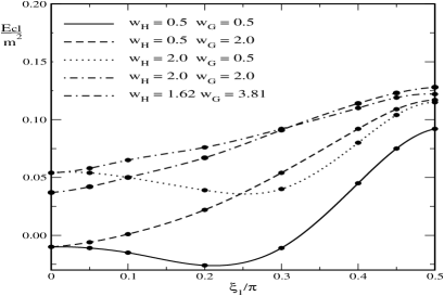
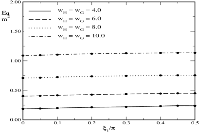
Figure 2: Vacuum polarization energy as function of the angle $\xi_{1}$ for different values of the width parameters $w_{H}$ and $w_{G}$ in the on–shell renormalization scheme. The physically motivated model parameters, eq. (4), are used. The dots refer to actual computations, while the lines stem from a cubic spline. We also show the results obtained for the fit to the Nielsen–Olesen profiles, cf. figure 1. These results do not include the combinatoric color factor $N_{C}$.

    

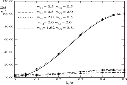
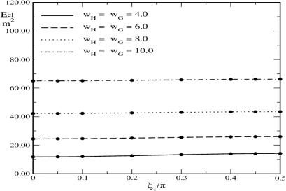
Figure 3: Classical energy for the standard model parameters as function of the ansatz parameters $w_{H}$, $w_{G}$ and $\xi_{1}$, including the fit to the Nielsen–Olesen profiles. The model parameters are again from eq. (4).

In figure 2 we show the result of this numerical computation. The wider the background fields, the weaker the dependence on the angle $\xi_{1}$ that parameterizes the gauge boson contribution. Surprisingly, we see that the vacuum polarization per unit length is quite small. Even for large widths it does not exceed a fraction of the fermion mass squared. With the exception of very small widths, the vacuum polarization turns out to be positive. Hence there is no indication that the vacuum polarization energy from the fermions can stabilize cosmic strings since the classical energy is larger by orders of magnitude, unless the coupling constants are $f,g\sim{\mathcal{O}}(10)$. For example, see figure 3, which shows the classical energy for the standard model parameters, which are ${\mathcal{O}}(1)$. The derivative terms of the classical energy decrease quadratically with $f$ and $g$ while the Higgs potential decreases like $1/f^{4}$ for fixed Higgs mass. As a result, increasing the coupling constants could lead to binding for thin strings, but such configurations contain large Fourier components, which for $f,g\sim{\cal O}(10)$ reach the vicinity of the Landau ghost pole. Hence any such binding is obscured by the existence of the Landau ghost, cf. appendix C.4, which arises when including quantum corrections in a manner that does not reflect asymptotic freedom. Here it is due to the omission of quantum corrections from fluctuating gauge boson fields. The estimate for the Landau ghost contribution discussed in the appendix suggests that the issue can be safely ignored for $f,g\lesssim 5$.

Gradient expansions Kir93 for quantum mechanical expectation values suggest that the energy gain from populating bound states can be estimated from a spatial integral over some fractional power of the potential in the wave–equation. Scaling arguments show that the energy from the populated bound states increases quadratically with the width parameters $w_{H}$ and/or $w_{G}$, regardless of the specific power in the expansion. Since also the dominating classical energy increases quadratically with $w_{H}$ (from the Higgs potential), populating the bound states might balance the large classical energy already at small coupling constants and moderate widths, because the Higgs potential scales like $1/f^{4}$ when the Higgs mass is fixed while the fermion contribution is not sensitive to any change in $f$ when we scale our definitions of physical quantities with the fermion mass $m=vf$. Hence our strategy to construct a stable string type configuration is to balance the classical boson energy with the fermion quantum correction by considering wide strings and increasing the Yukawa coupling. Simultaneously we must keep fixed the charge associated with populating the fermion bound states.

Before we will consider the total energy we would like to discuss the fermion part, $E_{\rm q}+E_{\rm b}$. In figure 4 we show the total fermion energy of eq. (19), as a function of the charge density per unit length of the string. As described in the previous section, we can compute the binding energy as a function of the charge for a given background configuration. After adding the vacuum polarization energy computed for that background, we get the parabolic curves in figure 4. These lines terminate at the point where all available bound states are populated. We then search for the configuration that minimizes the energy. For small charges, we obtain thin strings, while larger charges lead to wide strings, as shown in figure 4. Surprisingly, the resulting envelope that describes the minimal fermion energy as a function of the charge density is a straight line with (approximately) vanishing $y$–intercept. This straight line stems from a delicate balance between the vacuum polarization and binding energies. Because this extrapolation yields a vanishing $y$–intercept, we deduce that very narrow strings have vanishing vacuum polarization energy. This interpolation overcomes the Landau ghost problem of the direct calculation.

 

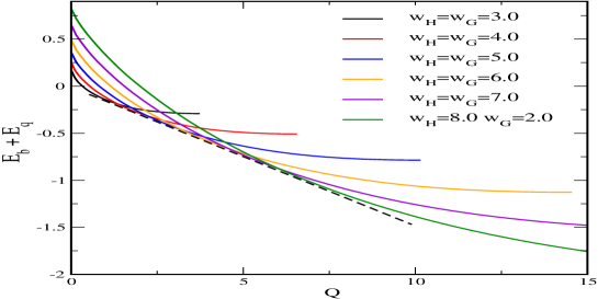
Figure 4: (Color online) Total bound state and vacuum energy per unit length as a function of charge density per unit length, in units of the fermion mass, for $\xi_{1}=0.4\pi$. The dotted line indicates the minimal fermionic contribution to the energy.

From several hundred configurations for which we have computed both the vacuum polarization energy and constructed the bound states, we identify the one that minimizes the total binding energy

$$E_{\rm tot}=E_{\rm cl}+E_{\rm q}+E_{\rm b}$$ (58)

for a prescribed charge. The corresponding result for the minimal binding energy is displayed in figure 5. We can see that the optimal binding grows linearly with $Q$. The steep slope at very small charges is an artifact of restricting our ansatz to configurations with $w_{H},w_{G}\geq 2$ to avoid unphysical effects from the Landau ghost.

As mentioned above, we increase the Yukawa coupling from its top–quark motivated value $f=0.99$, while all other model parameters are taken from eq. (4).

 

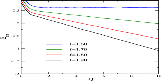
Figure 5: (Color online) Total energy as a function of the charge for various values of the Yukawa coupling constant. The color degeneracy $N_{C}=3$ is included.

Increasing the charge also increases the width of the optimal string. For $f\approx 1.6$ the classical and quantum contributions balance and the total energy is essentially independent of the width. Increasing the coupling further yields a negative energy (in comparison to equally many free fermions) and stable configurations exist. Not surprisingly, the minimal charge for which there are stable configurations decreases quickly as $f$ increases. For $f=1.7$ it is $Q_{\rm min}\sim 10m=17v$, while for $f=1.9$ stable configurations exist already at $Q_{\rm min}\sim 3m=5.7v$.

 

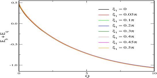
Figure 6: (Color online) Fermionic contribution to the string binding energy per unit length as a function of charge density per unit length, in units of the fermion mass, for a variety of values of $\xi_{1}$ with $w_{H}=6.0$ and $w_{G}=6.0$.

We next discuss the structure of the stabilizing configuration. We find that the fermionic part of the binding energy is insensitive to the angle $\xi_{1}$, as shown in figure 6. As a result, the dependence of the total binding energy on $\xi_{1}$ stems entirely from the classical part, which is clearly minimized for $\xi_{1}\sim 0$, since in that case the the gauge fields vanish and we have only a charged Higgs field, with only the non–diagonal elements in eq. (6) differing from zero.

In figure 7 we display the chemical potential that minimizes the binding energy for a prescribed charge. Its construction is discussed in section V.

 

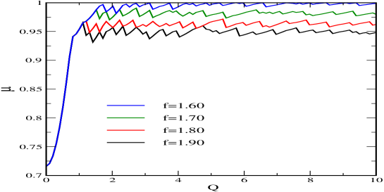
Figure 7: (Color online) The chemical potential that minimizes the binding energy for a prescribed charge in units of the fermion mass.

The cusps arise because our sample configurations are not continuous in the variational parameters. As we increase the charge, the minimizing configuration jumps among these possibilities.

The strong deviation from $\mu=m$ at low charges (where the various graphs overlap) is again an artifact of not considering very narrow string configurations. We see that at the limit of binding ($f=1.6$) almost all bound states are populated. As the binding increases, the chemical potential decreases, leaving the states below threshold un–occupied.

$f\Bigg{\backslash}Q$ 2 4 6 8 1.6 2.3 3.2 4.0 4.5 1.7 2.5 3.5 4.3 5.0 1.8 2.7 3.8 4.6 5.5 1.9 2.8 4.2 5.1 5.8

Table 1: The width, $w_{H}$, of the minimizing Higgs profile at a prescribed charge, $Q$ for different values of the Yukawa coupling constant $f$.

We have seen above that binding increases with the Yukawa coupling. Table 1 indicates that at the same time the profile functions get wider, while the critical charge at which binding sets in (i.e. $E_{\rm tot}(Q_{\rm min})=0$) decreases with the Yukawa coupling. As a result, the width of the critical profile actually decreases. We find these widths to be $5.5/m=3.2/v$, $4.0/m=2.2/v$ and $3.5/m=1.8/v$ for $f=1.7$, $1.8$ and $1.9$, respectively, and the typical extension of a bound charged string is about $0.003{\rm fm}$.

Finally let us estimate the total mass of the bound string. In the regime where it is only slightly bound, we have $E_{\rm tot}\lesssim Qm$. Typically we observe binding for $Q\approx 5m$. Hence a reasonable estimate for the mass of the string is $M\approx 5m^{2}L$. Taking $m=300{\rm GeV}$ and the length of the string to be the radius of the sun, $L=R_{\odot}\approx 7\times 10^{8}{\rm m}$ we find $M\approx 2.3\times 10^{9}{\rm kg}=10^{-20}M_{\odot}$, i.e. only a very tiny fraction of the mass of the sun. On the microscopic scale, a string as short as the Compton wave–length of the heavy fermion would carry about 30 bound fermions and have an energy of slightly less than $9{\rm TeV}$.

VII Conclusions

We have extended our previous spectral approach to find the leading quantum corrections to the energy of a cosmic string in a slightly simplified version of the electroweak theory. In the limit of many internal degrees of freedom, $N_{C}\to\infty$, these leading corrections come from fermions coupling to the string background. In this scenario $N_{C}$ merely appears a combinatoric factor, which is justified by the asymptotic freedom of QCD. We have shown how to compute the distortion of the Dirac spectrum in the string background, and how to extract the full non–perturbative renormalized vacuum polarization using perturbative counterterms and conventional renormalization schemes. Substantial refinements of our previous techniques were necessary to make this calculation feasible, and we have presented a complete account including technical details in the appendices. Though we have focused on the computational method underlying previously published results, we have also discussed some novel results concerning the structure of the stable configuration.

The basic idea of the quantum stabilization of cosmic strings is that the appearance of (near) zero modes in the distorted Dirac spectrum could help to produce negative contributions to the energy that overcomes the classical energy necessary to form the string. We have shown, however, that the contribution from the distortion of the remaining parts of the spectrum, i.e. the scattering states, neutralizes the binding effect of the low–lying modes, resulting in a very small vacuum polarization energy. In particular, the vacuum is stable against spontaneous formation of weak strings for parameters that are physically sensible. The situation is more favorable for charged strings with explicitly occupied bound states, since such configuration need only be lighter than the same number of free fermions, to be stable on time scales over which we may neglect fermion number nonconservation. This approximation is valid if the inter–generation quark mixing is tiny (we have assumed it to be zero), and if the quark masses in the heavy fermion doublet are nearly degenerate (we have assumed exact degeneracy).

For otherwise realistic parameters, we have shown that this binding mechanism sets in at surprisingly low fermion masses of around $300\,\mathrm{GeV}$. This corresponds to values of the Yukawa coupling that are still small enough for our calculations based on the Standard Model to be reliable. A stable charged string can thus be formed when enough charge density of a heavy fermion doublet with about twice the top quark mass is available.

If taken at face value, our findings suggest that a weakly coupled fourth generation of heavy quarks would make its footprint through the electroweak string phenomenology mentioned in the introduction — or conversely, that the non–observation of electroweak strings would put severe bounds on the masses of possible heavy quarks. However, such conclusions must be qualified by a number of simplifications that were necessary to make the calculation feasible. Most notably, the restriction to fermionic quantum fluctuations, although justified by the large $N_{C}$–argument, leads to a quantum theory that is not asymptotically free, and in turn to the Landau pole problem at small string widths. We have presented a crude way of estimating this contribution in order to ensure that our findings are not affected by it. This treatment should obviously be improved by a full quantum calculation of the bosonic contribution to the vacuum polarization energy. Recent studies Baacke:2008sq in models related to ours indicate that the bosonic contribution can give interesting and non–trivial effects. We are currently investigating such an extension of our model.

Other shortcomings of our model are the mass degeneracy of the fermion doublet, the lack of inter–generation quark couplings and, in particular, the decoupling of $U(1)$ hypercharge. While the stable configuration that we have constructed can be embedded in a full $SU(2)\times U(1)$ model with multiple generations (since additional degrees of freedom would only serve to lower the energy in our variational approach), it is unclear if the new couplings provide new decay channels, in particular when bosonic fluctuations are taken into account. We also plan to investigate such a scenario.

The charges along the string may carry currents Davis:1988jq ; Davis:1995kk ; Davis:1996xs , which in turn can have interesting consequences for baryogenesis and cosmology Davis:1999ec ; Lilley:2010av . This situation is similar to the Witten model Witten:1984eb ; Jackiw:1981ee and its generalizations, where the currents are induced by the coupling of extra scalar fields to the vortex. In this scenario, the Brownian network of vortices produced in an earlier (GUT-scale) phase transition contracts as the universe cools down. This process could eventually be stopped by the currents becoming superconducting, with the irregular vortex shapes being smoothed out by the surrounding thermal background to form circular rings. The final evolution stage would then be a universe filled with microscopic superconducting, charged vortex loops. Such a vorton Davis:1988ij ; Brandenberger:1996zp universe has recently attracted much attention because it provides a viable candidate for dark matter with rather accurately computable properties that put stringent restrictions on cosmological models. It would be very interesting to study such a possibility in the electroweak standard model, with currents produced directly from fermions (as they are in our calculation), rather than from extra scalar fields. Although our present investigation does not directly address this question, it seems conceivable that a stable vorton could be created without requiring exceedingly large couplings or unrealistic masses. Combining this scenario to our picture could be another avenue for future research.

Finally, it would of course also be interesting to study the Brownian network of strings as it is formed in the phase transition if enough fermion charge is available. Due to their complexity, such configurations must presumably be studied in an effective (lattice) model. The necessary string interactions could potentially be addressed through further extensions of the spectral method.

Appendix A Eigenvalue Problem

To find the bound state spectrum, states with energy eigenvalues $|\epsilon|<m$, we first diagonalize the Hamiltonian matrix in the absence of a background potential, and then use these free eigenstates (with the proper boundary conditions built in) as a basis in which to compute the matrix elements of the background potential induced by the string. The diagonalization of this full Hamiltonian matrix in turn yields the fully interacting bound state spectrum. Note that in this procedure all states appear as “bound” states, since the volume of the coordinate space is finite. In general the energy eigenvalues of such “bound” states depend on the volume. However, the true bound states with $|\epsilon|<m$ do not show finite size effects if the volume is chosen large enough because their wave–functions are located in a small sub–volume.

The single particle Dirac Hamiltonian couples spin ($S$) and weak isospin ($I$) degrees of freedom. We can combine these degrees of freedom by introducing the grand spin states given in eq. (12). The matrix elements of the (two–component) operators entering the Hamiltonians in eqs. (10) and (39) are listed in tables 3 to 7. In all of these tables, we use the abbreviation $s_{x}={\rm sin}(x)$ and $c_{x}={\rm cos}(x)$, where the arguments of these trigonometric functions appear as subscripts.

states $|++\rangle$ $|+-\rangle$ $|-+\rangle$ $|--\rangle$ $\langle++|$ 0 0 -1 0 $\langle+-|$ 0 0 0 -1 $\langle-+|$ 1 0 0 0 $\langle--|$ 0 1 0 0

Table 2: Matrix elements of $i\mbox{\boldmath$\sigma$\unboldmath}\cdot\widehat{\mbox{\boldmath$\rho$}}$. The table should be read as $\langle\,-+|\,i\mbox{\boldmath$\sigma$\unboldmath}\cdot\widehat{\mbox{\boldmath$\rho$}}\,|++\,\rangle=1$, for instance. The matrix is hermitian in combination with the derivative $\partial_{\rho}$.

states $|++\rangle$ $|+-\rangle$ $|-+\rangle$ $|--\rangle$ $\langle++|$ 0 0 $-(\ell+n+1)$ 0 $\langle+-|$ 0 0 0 $-(\ell+1)$ $\langle-+|$ $-(\ell+n)$ 0 0 0 $\langle--|$ 0 $-\ell$ 0 0

Table 3: Matrix elements of $i\,(\mbox{\boldmath$\sigma$\unboldmath}\cdot\widehat{\mbox{\boldmath$\varphi$}})\,\partial_{\varphi}$.

states $|++\rangle$ $|+-\rangle$ $|-+\rangle$ $|--\rangle$ $\langle++|$ 0 0 0 $1$ $\langle+-|$ 0 0 $-1$ 0 $\langle-+|$ 0 $-1$ 0 0 $\langle--|$ $1$ 0 0 0

Table 4: Matrix elements of $(\mbox{\boldmath$\sigma$\unboldmath}\cdot\widehat{\mbox{\boldmath$\rho$}})\,I_{P}$.

states $|++\rangle$ $|+-\rangle$ $|-+\rangle$ $|--\rangle$ $\langle++|$ 0 0 $-s_{\Delta}$ $-c_{\Delta}$ $\langle+-|$ 0 0 $-c_{\Delta}$ $s_{\Delta}$ $\langle-+|$ $-s_{\Delta}$ $-c_{\Delta}$ 0 0 $\langle--|$ $-c_{\Delta}$ $s_{\Delta}$ 0 0

Table 5: Matrix elements of $(\mbox{\boldmath$\sigma$\unboldmath}\cdot\widehat{\mbox{\boldmath$\varphi$}})\,I_{G}(\Delta)$. The subscript denotes the argument of the trigonometric functions.

states $|++\rangle$ $|+-\rangle$ $|-+\rangle$ $|--\rangle$ $\langle++|$ 0 0 $s_{\xi}$ $-c_{\xi}$ $\langle+-|$ 0 0 $-c_{\xi}$ $-s_{\xi}$ $\langle-+|$ $s_{\xi}$ $-c_{\xi}$ 0 0 $\langle--|$ $-c_{\xi}$ $-s_{\xi}$ 0 0

Table 6: Matrix elements of $(\mbox{\boldmath$\sigma$\unboldmath}\cdot\widehat{\mbox{\boldmath$\varphi$}})\,I_{G}(-\xi)$. The subscript denotes the argument of the trigonometric functions.

states $|++\rangle$ $|+-\rangle$ $|-+\rangle$ $|--\rangle$ $\langle++|$ 0 $1$ 0 0 $\langle+-|$ $-1$ 0 0 0 $\langle-+|$ 0 0 0 $1$ $\langle--|$ 0 0 $-1$ 0

Table 7: Matrix elements of $iI_{P}$. The extra factor $i$ leads to anti–hermitian matrix elements, compensating the same property of its spinor coefficient $\beta\gamma_{5}$.

Next, radial functions are introduced via the four–component spinors, cf. eq. (15),

$$~{}\hskip 56.9055pt\begin{array}[]{r@{\,\,\,=\,\,\,}l@{\qquad\longrightarrow\qquad}l}\displaystyle\langle\rho|\epsilon\,\ell++\rangle&\displaystyle{J_{\ell+n}(k\rho)|\ell++\rangle\choose\kappa J_{\ell+n+1}(k\rho)|\ell-+\rangle}&\displaystyle{f_{1}(\rho)|\ell++\rangle\choose g_{1}(\rho)|\ell-+\rangle}\\[17.07164pt] \displaystyle\langle\rho|\epsilon\,\ell+-\rangle&\displaystyle{J_{\ell}(k\rho)|\ell+-\rangle\choose\kappa J_{\ell+1}(k\rho)|\ell--\rangle}&\displaystyle{f_{2}(\rho)|\ell+-\rangle\choose g_{2}(\rho)|\ell--\rangle}\\[17.07164pt] \displaystyle\langle\rho|\epsilon\,\ell-+\rangle&\displaystyle{J_{\ell+n+1}(k\rho)|\ell-+\rangle\choose\kappa J_{\ell+n}(k\rho)|\ell++\rangle}&\displaystyle{f_{3}(\rho)|\ell-+\rangle\choose g_{3}(\rho)|\ell++\rangle}\\[17.07164pt] \displaystyle\langle\rho|\epsilon\,\ell--\rangle&\displaystyle{J_{\ell+1}(k\rho)|\ell--\rangle\choose\kappa J_{\ell}(k\rho)|\ell+-\rangle}&\displaystyle{f_{4}(\rho)|\ell--\rangle\choose g_{4}(\rho)|\ell+-\rangle}\,.\hskip 62.59596pt\mbox{(59)}\end{array}$$

We note that $\kappa={\rm sgn}(\epsilon)\,\sqrt{\frac{\epsilon-m}{\epsilon+m}}$ is well defined for either sign of the energy eigenvalue since $|\epsilon|>m$. Using the dispersion relation for real momenta $\epsilon^{2}=k^{2}+m^{2}$, we may also write $\kappa=\frac{k}{\epsilon+m}=\frac{\epsilon-m}{k}$. These two expressions are odd in $k$ and thus suitable for analytic continuation $k\to it$. The spinors to the left of the arrows in eq. (A) involve ordinary Bessel functions which solve the free Dirac equation. They will be used to construct the basis states for the Hamiltonian matrix.

In the free case, the four spinors in eq. (A) each solve the Dirac equation individually, i.e. they do not couple. Once the background potential from the string is included, however, the radial functions $f_{i}$ and $g_{i}$ become distorted and mix under the dynamics.

We now construct a discrete basis built from solutions of the free Dirac equation. To this end we must first impose the boundary condition that no flux runs from the center of the string through a circle at a large distance $R$. Since the flux is bilinear in the spinors with all products involving both an upper and a lower component, the no–flux boundary condition is equivalent to the requirement that either component vanishes. For the string winding $n=1$, this amounts to the simple statement

$$J_{\ell+1}(k_{r}^{(\ell)}R)=0\,.$$ (60)

This conditions selects discrete momenta $k_{r}^{(\ell)}$ in each angular momentum channel $\ell$, where $r=1,2,\ldots$ enumerates the momenta and thus the free basis states. We note in passing that a string winding $n\geq 2$ would require two separate sets of discrete momenta.

The normalization of the spinors can be worked out using the Bessel function identity

$$\int_{0}^{1}tdtJ_{\nu}(\lambda_{r}^{(\nu)}t)J_{\nu}(\lambda_{s}^{(\nu)}t)=\frac{1}{2}\left[J_{\nu}^{\prime}(\lambda_{r}^{(\nu)}t)\right]^{2}\delta_{rs}$$ (61)

where $\lambda_{r}^{(\nu)}$ are the roots of the Bessel function $J_{\nu}$. Using furthermore the recursion relations for Bessel functions and their derivatives, we arrive at the following explicit expressions for the (free) radial functions in equation (15),

$$f_{1}^{(r)}(\rho)$$ = =

= =

= =

= =

(62)

where the superscripts on the momenta are omitted. The normalization factors are given explicitly by

$$N_{f}^{(r)}=\frac{1}{R}\frac{1}{|J_{\ell+2}(k_{r}R)|}\sqrt{\frac{\epsilon_{r}+m}{\epsilon_{r}}}\,,\quad\qquad N_{g}^{(r)}=\frac{1}{R}\frac{{\rm sgn}(\epsilon_{r})}{|J_{\ell+2}(k_{r}R)|}\sqrt{\frac{\epsilon_{r}-m}{\epsilon_{r}}}\,.$$ (63)

To limit the number of basis states, we introduce a cutoff $\Lambda$ and only include momenta with $k_{r}<\Lambda$. This defines $r_{\rm max}$, the maximal number of discrete momenta, which depends on $R$ for fixed $\Lambda$. Due to the energy degeneracy this cutoff truncates the label $r$ on the energy eigenvalues to run from $1\ldots 2r_{\max}$,

$$\epsilon_{r}=\begin{cases}-\sqrt{k_{r_{\rm max}+1-r}^{2}+m^{2}}&\quad r=1,\ldots,r_{\rm max}\\[11.38109pt] \sqrt{k_{r-r_{\rm nmax}}^{2}+m^{2}}&\quad r=r_{\rm max}+1,\ldots,2r_{\rm max}\,.\end{cases}$$ (64)

Putting all the pieces together, we can now present the full Hamiltonian matrix i.e. the operator in eq. (10) sandwiched between the spinors constructed above. The equations become simpler if we set

$$C_{\pm}=c_{\Delta}\alpha_{G}+c_{\xi}\alpha_{\xi}\pm\alpha_{r}\qquad{\rm and}\qquad S=s_{\Delta}\alpha_{G}-s_{\xi}\alpha_{\xi}\,,$$ (65)

with the right hand sides containing the elements of $V_{i}$ in eq. (17). They are specified in terms of the string profile functions in eq. (90) of the following appendix. The interaction Hamiltonian matrix elements read

$$\langle 1r|H_{\rm int}|1s\rangle = \alpha_{H}\left(f_{1}^{(r)}f_{1}^{(s)}-g_{1}^{(r)}g_{1}^{(s)}\right)-S\left(f_{1}^{(r)}g_{1}^{(s)}+g_{1}^{(r)}f_{1}^{(s)}\right)$$ (66)

$$\langle 2r|H_{\rm int}|1s\rangle = -C_{+}f_{2}^{(r)}g_{1}^{(s)}-C_{-}g_{2}^{(r)}f_{1}^{(s)}$$ (67)

$$\langle 3r|H_{\rm int}|1s\rangle = S\left(f_{3}^{(r)}f_{1}^{(s)}+g_{3}^{(r)}g_{1}^{(s)}\right)$$ (68)

$$\langle 4r|H_{\rm int}|1s\rangle = C_{-}f_{4}^{(r)}f_{1}^{(s)}+C_{+}g_{4}^{(r)}g_{1}^{(s)}-\alpha_{P}\left(f_{4}^{(r)}g_{1}^{(s)}-g_{4}^{(r)}f_{1}^{(s)}\right)$$ (69)

$$\langle 1r|H_{\rm int}|2s\rangle = -C_{-}f_{1}^{(r)}g_{2}^{(s)}-C_{+}g_{1}^{(r)}f_{2}^{(s)}$$ (71)

$$\langle 2r|H_{\rm int}|2s\rangle = \alpha_{H}\left(f_{2}^{(r)}f_{2}^{(s)}-g_{2}^{(r)}g_{2}^{(s)}\right)+S\left(f_{2}^{(r)}g_{2}^{(s)}+g_{2}^{(r)}f_{2}^{(s)}\right)$$ (72)

$$\langle 3r|H_{\rm int}|2s\rangle = C_{+}f_{3}^{(r)}f_{2}^{(s)}+C_{-}g_{3}^{(r)}g_{2}^{(s)}+\alpha_{P}\left(f_{3}^{(r)}g_{2}^{(s)}-g_{3}^{(r)}f_{2}^{(s)}\right)$$ (73)

$$\langle 4r|H_{\rm int}|2s\rangle = -S\left(f_{4}^{(r)}f_{2}^{(s)}+g_{4}^{(r)}g_{2}^{(s)}\right)$$ (74)

$$\langle 1r|H_{\rm int}|3s\rangle = S\left(f_{1}^{(r)}f_{3}^{(s)}+g_{1}^{(r)}g_{3}^{(s)}\right)$$ (76)

$$\langle 2r|H_{\rm int}|3s\rangle = C_{+}f_{2}^{(r)}f_{3}^{(s)}+C_{-}g_{2}^{(r)}g_{3}^{(s)}-\alpha_{P}\left(f_{2}^{(r)}g_{3}^{(s)}-g_{2}^{(r)}f_{3}^{(s)}\right)$$ (77)

$$\langle 3r|H_{\rm int}|3s\rangle = \alpha_{H}\left(f_{3}^{(r)}f_{3}^{(s)}-g_{3}^{(r)}g_{3}^{(s)}\right)-S\left(f_{3}^{(r)}g_{3}^{(s)}+g_{3}^{(r)}f_{3}^{(s)}\right)$$ (78)

$$\langle 4r|H_{\rm int}|3s\rangle = -C_{-}f_{4}^{(r)}g_{3}^{(s)}-C_{+}g_{4}^{(r)}f_{3}^{(s)}$$ (79)

$$\langle 1r|H_{\rm int}|4s\rangle = C_{-}f_{1}^{(r)}f_{4}^{(s)}+C_{+}g_{1}^{(r)}g_{4}^{(s)}+\alpha_{P}\left(f_{1}^{(r)}g_{4}^{(s)}-g_{1}^{(r)}f_{4}^{(s)}\right)$$ (81)

$$\langle 2r|H_{\rm int}|4s\rangle = -S\left(f_{2}^{(r)}f_{4}^{(s)}+g_{2}^{(r)}g_{4}^{(s)}\right)$$ (82)

$$\langle 3r|H_{\rm int}|4s\rangle = -C_{+}f_{3}^{(r)}g_{4}^{(s)}-C_{-}g_{3}^{(r)}f_{4}^{(s)}$$ (83)

$$\langle 4r|H_{\rm int}|4s\rangle = \alpha_{H}\left(f_{4}^{(r)}f_{4}^{(s)}-g_{4}^{(r)}g_{4}^{(s)}\right)+S\left(f_{4}^{(r)}g_{4}^{(s)}+g_{4}^{(r)}f_{4}^{(s)}\right)\,.$$ (84)

To keep the presentation simple we have omitted the radial integrals on the right hand sides, i.e. they are understood to be integrated with $\int_{0}^{R}\rho\,d\rho\,\left(\ldots\right)$. In total this defines $8r_{\rm max}\times 8r_{\rm max}$ matrix elements of the interaction Hamiltonian. To populate the full Hamiltonian matrix, we set

$$H^{(I)}_{r+2r_{\rm max},s}=\langle 2r|H_{\rm int}|1s\rangle$$ (85)

for $r,s=1,\ldots,2r_{\rm max}$, and $\epsilon_{r+2qr_{\rm max}}=\epsilon_{r}$ for $q=1,2,3$. This yields the $8r_{\rm max}\times 8r_{\rm max}$ matrix

$$H_{r,s}=\epsilon_{r}\delta_{rs}+H^{(I)}_{r,s}\qquad r,s=1,\ldots,8r_{\rm max}\,,$$ (86)

which is diagonalized numerically by means of a Jacobi routine.

Once the radius $R$ and the momentum cutoff $\Lambda$ are large enough the true bound state spectrum should become stable against further increase of these parameters. Typical values are $\Lambda\approx 8m$ and $R=75/m$, so that our free basis comprises about 400 energy eigenvalues, each with fourfold degeneracy and the Hamiltonian matrix has $1600\times 1600$ entries for the lowest angular momentum. For wider string profiles, bound states occur in higher and higher angular momentum channels. For instance, bound states appear for up to $\ell=5$ when $w_{H}\approx 6/m$, while narrow widths $w_{H}\leq 1/m$ only induce bound states in the channel $\ell=-n=-1$, i.e. the effective $S$–wave channel.

We have verified the gauge independence of the bound state energies by checking that they are insensitive to variations in the shape of the gauge transformation profile $\xi(\rho)$. Also the zero mode in the $\ell=-n=-1$ channel is observed for $\xi_{1}=\nicefrac{{\pi}}{{2}}$ regardless of the values of the width parameters.

Appendix B Scattering problem

In this appendix we describe the scattering solutions to the Dirac equation (17). To this end we write the Dirac Hamiltonian, eq. (10) in terms of $4\times 4$ matrices and derive the differential equation for the Jost function.

B.1 Differential equation for Jost function

The derivative operators as well as the angular barriers are contained in the diagonal $4\times 4$ matrices

$$D_{u} \equiv \partial_{\rho}\,\mbox{{\sf 1}\mbox{}\rule{0.39993pt}{6.6736pt}\mbox{\hskip 1.00006pt}}-\frac{1}{\rho}\,\mathrm{diag}\big{(}-(\ell+n+1)\,,\,-(\ell+1)\,,\,\ell+n\,,\,\ell\big{)}$$

$$D_{d} \equiv \partial_{\rho}\,\mbox{{\sf 1}\mbox{}\rule{0.39993pt}{6.6736pt}\mbox{\hskip 1.00006pt}}-\frac{1}{\rho}\,\mathrm{diag}\big{(}\ell+n\,,\,\ell\,,\,-(\ell+n+1)\,,\,-(\ell+1)\big{)}$$ (87)

where $C=\mathrm{diag}(-1,-1,1,1)$. For the interactions, we must compute the matrix elements of the various pieces in eq. (10) within the grand spin basis eq. (12). The explicit expressions for the emerging radial functions are listed in eqs. (15) and (16), cf. eq. (A). After some lengthy algebra, the interaction matrices in the system (17) can written in terms of simpler sub–matrices,

$$\begin{array}[]{ll}V_{uu}=\begin{pmatrix}H&G_{+}\cr G_{-}&H\end{pmatrix}&\qquad V_{dd}=\begin{pmatrix}-H&G_{-}\cr G_{+}&-H\end{pmatrix}\cr\cr V_{ud}=-\begin{pmatrix}G_{+}&P\cr P&G_{-}\end{pmatrix}&\qquad V_{du}=-\begin{pmatrix}G_{-}&-P\cr-P&G_{+}\end{pmatrix}\,,\end{array}$$ (88)

where the $2\times 2$ submatrices are

$$H = \alpha_{H}\,\begin{pmatrix}1&0\cr 0&1\end{pmatrix}\,,\qquad\qquad P=\alpha_{p}\,\begin{pmatrix}0&-1\cr 1&0\end{pmatrix}\,,$$

$$G_{\pm} = \alpha_{G}\,\begin{pmatrix}\sin\Delta&\cos\Delta\cr\cos\Delta&-\sin\Delta\end{pmatrix}+\alpha_{\xi}\,\begin{pmatrix}-\sin\xi&\cos\xi\cr\cos\xi&\sin\xi\end{pmatrix}\pm\alpha_{r}\,\begin{pmatrix}0&-1\cr 1&0\end{pmatrix}\,.$$ (89)

The coefficients $\alpha_{H}$, $\alpha_{p}$, $\alpha_{G}$, $\alpha_{\xi}$ and $\alpha_{r}$ are radial functions determined by the background profiles $f_{G},f_{H}$ and the gauge function $\xi$,

$$\alpha_{r}(\rho) = \frac{1}{2}\,\frac{\partial\xi(\rho)}{\partial\rho}$$

$$\alpha_{G}(\rho) = \frac{n}{2\rho}\,f_{G}(\rho)\,\sin\Delta(\rho)$$

$$\alpha_{\xi}(\rho) = \frac{n}{2\rho}\,\big{(}f_{G}(\rho)-1\big{)}\,\sin\xi(\rho)$$

$$\alpha_{H}(\rho) = m\,\big{(}f_{H}(\rho)\,\cos\Delta(\rho)-1\big{)}$$

$$\alpha_{P}(\rho) = mf_{H}(\rho)\,\sin\Delta(\rho)\,.$$ (90)

Note that the new gauge function also enters via $\Delta(\rho)\equiv\xi_{1}-\xi(\rho)$. We now write the Dirac equation for the matrix fields defined in eq. (25) as

$$\partial_{\rho}\mathcal{F} = \left[\overline{\mathcal{M}}_{ff}+O_{d}\right]\cdot\mathcal{F}+\mathcal{F}\cdot\mathcal{M}_{ff}^{(r)}+\left[\overline{\mathcal{M}}_{fg}+kC\right]\cdot\mathcal{G}\cdot Z_{d}$$ (91)

$$\partial_{\rho}\mathcal{G} = \left[\overline{\mathcal{M}}_{gg}+O_{u}\right]\cdot\mathcal{G}+\mathcal{G}\cdot\mathcal{M}_{gg}^{(r)}+\left[\overline{\mathcal{M}}_{gf}-kC\right]\cdot\mathcal{F}\cdot Z_{u}\,,$$ (92)

where the $4\times 4$ matrices without an overline are purely kinematic,

$$Z_{u} = {\rm diag}\,\left(\frac{H_{\ell+n}(k\rho)}{H_{\ell+n+1}(k\rho)}\,,\frac{H_{\ell}(k\rho)}{H_{\ell+1}(k\rho)}\,,\frac{H_{\ell+n+1}(k\rho)}{H_{\ell+n}(k\rho)}\,,\frac{H_{\ell+1}(k\rho)}{H_{\ell}(k\rho)}\right)$$

$$Z_{d} = {\rm diag}\,\left(\frac{H_{\ell+n+1}(k\rho)}{H_{\ell+n}(k\rho)}\,,\frac{H_{\ell+1}(k\rho)}{H_{\ell}(k\rho)}\,,\frac{H_{\ell+n}(k\rho)}{H_{\ell+n+1}(k\rho)}\,,\frac{H_{\ell}(k\rho)}{H_{\ell+1}(k\rho)}\right)=\left(Z_{u}\right)^{-1}$$

$$O_{u} = \frac{1}{\rho}\,{\rm diag}\,\left(-(\ell+n+1),-(\ell+1),\ell+n,\ell\right)$$

$$O_{d} = \frac{1}{\rho}\,{\rm diag}\,\left(\ell+n,\ell,-(\ell+n+1),-(\ell+1)\right)$$

$$C = \mathrm{diag}(-1,-1,1,1)\,.$$ (93)

The matrices multiplying $\mathcal{F}$ and $\mathcal{G}$ from the right are also independent of the background potential,

$$\mathcal{M}_{ff}^{(r)}=-kC\cdot Z_{d}-O_{d}\qquad{\rm and}\qquad\mathcal{M}_{gg}^{(r)}=kC\cdot Z_{u}-O_{u}\,.$$ (94)

Genuine interactions from the string background are solely contained in the overlined matrices in eq. (92). Using the same $2\times 2$ matrix notation as above, we have explicitly

$$\begin{array}[]{ll}\overline{\mathcal{M}}_{gg}=CV_{ud}=\begin{pmatrix}G_{+}&P\cr-P&-G_{-}\end{pmatrix}&\qquad\overline{\mathcal{M}}_{ff}=-CV_{du}=\begin{pmatrix}-G_{-}&P\cr-P&G_{+}\end{pmatrix}\cr\cr\overline{\mathcal{M}}_{gf}=\frac{1}{\kappa}CV_{uu}=\frac{1}{\kappa}\begin{pmatrix}-H&-G_{+}\cr G_{-}&H\end{pmatrix}&\qquad\overline{\mathcal{M}}_{fg}=-\kappa CV_{dd}=\kappa\begin{pmatrix}-H&G_{-}\cr-G_{+}&H\end{pmatrix}\,.\end{array}$$ (95)

The solutions to the differential equations (92) subject to the boundary conditions $\mathcal{F}\to\mbox{{\sf 1}\mbox{}\rule{0.39993pt}{6.6736pt}\mbox{\hskip 1.00006pt}}$ and $\mathcal{G}\to\mbox{{\sf 1}\mbox{}\rule{0.39993pt}{6.6736pt}\mbox{\hskip 1.00006pt}}$ at $\rho\to\infty$ define the scattering solution, eq. (27), from which we extract the scattering matrix as described in eq. (29).

B.2 Born series

To set up the Born series defined in eq. (30), we simply expand the system of differential equations from the last section in powers of the background potential, which only enters the overlined matrices. At first order, we obtain

$$\partial_{\rho}\mathcal{F}^{(1)} = O_{d}\cdot\mathcal{F}^{(1)}+\mathcal{F}^{(1)}\cdot\mathcal{M}_{ff}^{(r)}+kC\cdot\mathcal{G}^{(1)}\cdot Z_{d}+\overline{\mathcal{M}}_{ff}+\overline{\mathcal{M}}_{fg}\cdot Z_{d}$$ (96)

$$\partial_{\rho}\mathcal{G}^{(1)} = O_{u}\cdot\mathcal{G}^{(1)}+\mathcal{G}^{(1)}\cdot\mathcal{M}_{gg}^{(r)}-kC\cdot\mathcal{F}^{(1)}\cdot Z_{u}+\overline{\mathcal{M}}_{gg}+\overline{\mathcal{M}}_{gf}\cdot Z_{u}\,.$$ (97)

The matrices $\mathcal{M}_{\ldots}^{(r)}$ do not contain the interactions and are thus of order zero. In the same way we obtain the second order equations,

$$\partial_{\rho}\mathcal{F}^{(2)} = O_{d}\cdot\mathcal{F}^{(2)}+\mathcal{F}^{(2)}\cdot\mathcal{M}_{ff}^{(r)}+kC\cdot\mathcal{G}^{(2)}\cdot Z_{d}+\overline{\mathcal{M}}_{ff}\cdot\mathcal{F}^{(1)}+\overline{\mathcal{M}}_{fg}\cdot\mathcal{G}^{(1)}\cdot Z_{d}$$ (98)

$$\partial_{\rho}\mathcal{G}^{(2)} = O_{u}\cdot\mathcal{G}^{(2)}+\mathcal{G}^{(2)}\cdot\mathcal{M}_{gg}^{(r)}-kC\cdot\mathcal{F}^{(2)}\cdot Z_{u}+\overline{\mathcal{M}}_{gg}\cdot\mathcal{G}^{(1)}+\overline{\mathcal{M}}_{gf}\cdot\mathcal{F}^{(1)}\cdot Z_{u}\,.$$ (99)

With these Jost–like matrices, the Born series for the $S$–matrix is $\mathcal{S}=\mbox{{\sf 1}\mbox{}\rule{0.39993pt}{6.6736pt}\mbox{\hskip 1.00006pt}}+\mathcal{S}^{(1)}+\mathcal{S}^{(2)}+\ldots\,$ with

$$\mathcal{S}^{(1)} = \lim_{\rho\to 0}\left\{\mathcal{H}_{u}^{-1}\cdot\left[\mathcal{F}^{(1)^{*}}-\mathcal{F}^{(1)}\right]\cdot\mathcal{H}_{u}^{*}\right\}\,$$

$$\mathcal{S}^{(2)} = \lim_{\rho\to 0}\left\{\mathcal{H}_{u}^{-1}\cdot\left[\mathcal{F}^{(1)}\cdot\left(\mathcal{F}^{(1)}-\mathcal{F}^{(1)^{*}}\right)+\mathcal{F}^{(2)^{*}}-\mathcal{F}^{(2)}\right]\cdot\mathcal{H}_{u}^{*}\right\}$$ (100)

and similarly for $\mathcal{G}_{i}$ with $\mathcal{H}_{u}\to\mathcal{H}_{d}$. The Born expanded eigenphase shifts are now simply given, to first and second order, by

$$\delta_{\ell}^{(1)}=-\frac{1}{2}\,{\rm tr}\left[{\sf Im}\left(\mathcal{S}^{(1)}_{1}\right)\right]\qquad{\rm and}\qquad\delta_{\ell}^{(2)}=-\frac{1}{4}\,{\rm tr}\left[{\sf Im}\left(\mathcal{S}^{(1)}\cdot\mathcal{S}^{(1)}+2\mathcal{S}^{(2)}\right)\right]\,.$$ (101)

The third and fourth order pieces will be treated as part of the fake boson formalism discussed below in section C.2.

B.3 Analytic continuation

We describe the continuation to imaginary momenta for the case where $\epsilon=\sqrt{k^{2}+m^{2}}$; the second Riemann sheet ($\epsilon=-\sqrt{k^{2}+m^{2}}$) works analogously. The analytic continuation concerns the Hankel functions, which turn into modified Bessel functions, $Z_{u}\to Y_{u}$ and $Z_{d}\to Y_{d}$, with

$$Y_{u}={\rm diag}\,\left(\frac{K_{\ell+n}(t\rho)}{K_{\ell+n+1}(t\rho)}\,,\frac{K_{\ell}(t\rho)}{K_{\ell+1}(t\rho)}\,,-\frac{K_{\ell+n+1}(t\rho)}{K_{\ell+n}(t\rho)}\,,-\frac{K_{\ell+1}(t\rho)}{K_{\ell}(t\rho)}\right)=-\left(Y_{d}\right)^{-1}\,.$$ (102)

Furthermore, the kinematic coefficient turns into a pure phase

$$\kappa\to z_{\kappa}=\frac{m+i\sqrt{t^{2}-m^{2}}}{t}\,.$$ (103)

The system of differential equations for imaginary momentum then becomes

$$\partial_{\rho}\mathcal{F} = \left[\overline{\mathcal{M}}_{ff}+O_{d}\right]\cdot\mathcal{F}+\mathcal{F}\cdot\mathcal{M}_{ff}^{(r)}+\left[\overline{\mathcal{M}}_{fg}-tC\right]\cdot\mathcal{G}\cdot Y_{d}$$ (104)

$$\partial_{\rho}\mathcal{G} = \left[\overline{\mathcal{M}}_{gg}+O_{u}\right]\cdot\mathcal{G}+\mathcal{G}\cdot\mathcal{M}_{gg}^{(r)}+\left[\overline{\mathcal{M}}_{gf}+tC\right]\cdot\mathcal{F}\cdot Y_{u}\,.$$ (105)

with the boundary conditions that $\mathcal{F}$ and $\mathcal{G}$ both approach unity at $\rho\to\infty$. For simplicity, we have omitted the momentum arguments in the radial wave–functions $\mathcal{F}$ and $\mathcal{G}$ and also used the same symbol as in the case of real momenta, eqs. (92). The coefficient matrices in the differential equations are slightly modified:

$$\begin{array}[]{ll}\mathcal{M}_{gg}^{(r)}=-t\,C\cdot Y_{u}-O_{u}&\qquad\mathcal{M}_{ff}^{(r)}=t\,C\cdot Y_{d}-O_{d}\\[5.69054pt] \overline{\mathcal{M}}_{gf}=z_{\kappa}\begin{pmatrix}-H&-G_{+}\cr G_{-}&H\end{pmatrix}&\qquad\overline{\mathcal{M}}_{fg}=-z_{\kappa}^{*}\begin{pmatrix}-H&G_{-}\cr-G_{+}&H\end{pmatrix}\,,\end{array}$$ (106)

while $\overline{\mathcal{M}}_{gg}$ and $\overline{\mathcal{M}}_{ff}$ are the same as on the real axis.

Unlike the Schrödinger problem, the differential equations in the present case do not become real on the imaginary axis. Rather, charge conjugation $\epsilon\to-\epsilon$ induces complex conjugation. It is therefore not surprising that the naïve extrapolation $\lim_{\rho\to 0}\det(\mathcal{F})$ does not give a real result. Instead, we find numerically that $F=G^{*}$ with the imaginary part being independent of angular momentum for a given value of $t$. The origin for this imaginary part lies in the subtle definition of the Jost function via the Wronskian between the Jost solution, i.e. $\mathcal{F}$ or $\mathcal{G}$, and the regular solution, which satisfies momentum independent boundary conditions at the origin. The momentum independence of these boundary conditions ensures that the regular solution is an analytic function of complex momentum. Analyticity of the Jost solution, on the other hand, is guaranteed by the non–singular behavior of the interaction potentials, which is in turn a consequence of the boundary conditions on the profile function $\xi(\rho)$. At the origin, the Higgs field differs from its vacuum expectation value (it actually vanishes), which modifies the relative weight of the upper and lower Dirac components. More precisely, the non–diagonal elements of the matrices in eq. (106) vanish at the origin and the eight differential equations decouple with respect to the spin and weak isospin index on the radial functions in eq. (16). For real momenta $k$, a typical solution in the vicinity of $\rho=0$ then looks like Bordag:2003at

$$\begin{pmatrix}f_{4}\cr g_{4}\end{pmatrix}\sim\left(\frac{k}{q}\right)^{l}\begin{pmatrix}\sqrt{E+mc_{\Delta}f_{H}(0)}\,J_{l}(q\rho)\cr\cr\sqrt{E-mc_{\Delta}f_{H}(0)}\,J_{l+1}(q\rho)\end{pmatrix}$$ (107)

with $q=\sqrt{E^{2}-(mc_{\Delta}f_{H}(0))^{2}}$ and similar dependencies for the other six radial functions. The square–root coefficients cause the proper definition of the logarithmic Jost function, $\nu(t)$, to be

$${\rm exp}\left[\nu(t)\right]=\left(\frac{\tau-im}{\tau-imc_{\Delta}f_{H}(0)}\right)^{2}\lim_{\rho\to 0}{\rm det}(\mathcal{F})=\left(\frac{\tau+im}{\tau+imc_{\Delta}f_{H}(0)}\right)^{2}\lim_{\rho\to 0}{\rm det}(\mathcal{G})$$ (108)

with $\tau=\sqrt{t^{2}-m^{2}}$. The power of two occurs because we compute the determinant of a $4\times 4$ matrix. Notice that this redefinition not only cancels the imaginary parts, but also modifies the real part. Furthermore it avoids the logarithmic singularity in ${\rm ln}\left[\lim_{\rho\to 0}{\rm det}(\mathcal{F})\right]$ otherwise observed numerically at $t\sim m$. Since $f_{H}$ is part of the interaction, the correction prefactor in eq. (108) also contributes to the Born series. To make this explicit, we write

$${\rm ln}\left(\frac{\tau-im}{\tau-imc_{\Delta}f_{H}(0)}\right) = {\rm ln}\left(\frac{\tau-im}{\tau-i(\alpha_{H}(0)+m)}\right)$$ (109)

$$= \frac{i\alpha_{H}(0)}{\tau-im}-\frac{1}{2}\left(\frac{\alpha_{H}(0)}{\tau-im}\right)^{2}+\ldots\,,$$ (110)

and subsequently set $\alpha_{H}(0)=-m$. The Born expansion of the remaining determinant in eq. (108) is constructed as for real momenta by iterating the differential equation (105) in the interaction $\overline{\mathcal{M}}_{i}$.

Numerically, we integrate the differential equations (92), (105), their Born expansions and the fake boson analog

$$\partial_{\rho}^{2}\overline{\nu}_{\ell}(t,\rho)=2tL_{\ell}(t\rho)\partial_{\rho}\overline{\nu}_{\ell}(t,\rho)-\overline{\nu}_{\ell}^{2}(t,\rho)+V(\rho)\quad\mbox{with}\quad L_{\ell}(z)=\frac{K_{\ell+1}(z)}{K_{\ell}(z)}-\frac{\ell+\frac{1}{2}}{z}\,$$ (111)

from some large radius $\rho_{\rm max}\sim 4\rho_{0}$ to $\rho_{\rm min}\sim 0$ with the boundary condition $\mathcal{F}(\rho_{\rm max},k)=\mbox{{\sf 1}\mbox{}\rule{0.39993pt}{6.6736pt}\mbox{\hskip 1.00006pt}}$, and identify $\lim_{\rho\to 0}\mathcal{F}(\rho,k)=\mathcal{F}(\rho_{\rm min},k)$. Alternatively, this identification can also be obtained from the derivative of the wave–function. Furthermore, a differential equation is formulated for ${\rm ln}\,{\rm det}\mathcal{F}(\rho,k)^{-1}\mathcal{F}(\rho,k)^{\ast}$ to avoid $2\pi$ ambiguities in the computation of the phase shift, $\delta_{\ell}(k)$, cf. eq. (35).

The computations for real momenta have been performed mainly for use in the consistency tests on the unitarity of the scattering matrix and the spectral sum rules Graham:2001iv . There is one more merit of considering real momenta: Channels that include Hankel functions with zero index ($\ell=-2,-1,0$) are particularly cumbersome because regular and irregular solutions are difficult to separate in such cases, because they go as a constant and ${\rm ln}(\rho)$, respectively, at $\rho_{\rm min}\ll 1$, cf. eq. (29). As a consequence, $\rho_{\rm min}$ must be taken tiny in the problematic channels to obtain the correct scattering matrix in eq. (29). On the real axis, the result can be checked against extracting the $\mathcal{S}$–matrix from the derivative of the scattering wave–function because $Y_{0}^{\prime}(\rho)\sim Y_{1}(\rho)$ diverges like a power. For calculations on the imaginary axis, we assume $\rho_{\rm min}\sim 10^{-60}$ and successively carry out an extrapolation

$$\nu(\rho_{\rm min})=\nu_{0}+\frac{a_{1}}{{\rm ln}(\rho_{\rm min})}+\frac{a_{2}}{{\rm ln}^{2}(\rho_{\rm min})}\ldots\,\,,$$ (112)

for the Jost function in these channels. We test the final result, i.e. $\nu_{0}$, for stability against further changes of $\rho_{\rm min}$ and also check the condition ${\sf Im}(\nu_{0})=0$. In the non–problematic channels $\ell\notin\{-2,-1,0\}$, it is sufficient to set $\rho_{\rm min}\sim 10^{-12}$ in order to represent the origin.

We have also successfully tested our numerical results of the scattering data against the reflection symmetry $\ell\to-(\ell+2n)$.

Appendix C Feynman diagrams

In this appendix we describe the details of the computation of the Feynman diagrams. We start from the series in equation (42). This computation involves three parts:

1. The contribution linear in $H_{I}$. This term vanishes identically with the no–tadpole condition.

2. The piece quadratic in $H_{I}$. This term is quadratically divergent at high momenta and must be carefully regularized to handle the leading and subleading logarithmic divergences.

3. The contribution from terms cubic and quartic in $H_{I}$. They are only logarithmicly divergent which makes the separation of the finite parts simpler. Since the corresponding Feynman diagrams are complicated to evaluate we employ the fake boson methods to compute this part of the vacuum polarization energy.

We first consider the $\overline{\rm MS}$ scheme in which only the bare divergences proportional to

$$-i\left(\frac{\mu}{m}\right)^{4-D}\int\frac{d^{D}l}{(2\pi)^{D}}\left(l^{2}-1+i\epsilon\right)^{-2}\,,$$

are subtracted, and then determine the finite counterterm coefficients suitable to implement the on–shell renormalization scheme.

C.1 Second order contribution

After imposing the no–tadpole condition we find the contribution to the action functional up to second order in $H_{I}$ within the $\overline{\rm MS}$ scheme as

$$\Delta\mathcal{A} = -\frac{1}{8\pi^{2}}\int\frac{d^{4}k}{(2\pi)^{4}}\int_{0}^{1}dx\,{\rm ln}\left[1-x(1-x)\frac{k^{2}}{m^{2}}\right]$$ (117)

$$\hskip 5.69046pt\times{\rm tr}_{I}\Big{\{}\left[m^{2}-x(1-x)k^{2}\right]\left[\frac{1}{2}L(k)\cdot L(-k)-3\left(h(k)h(-k)+p(k)p(-k)\right)\right]$$

$$\hskip 42.67912pt+x(1-x)\left[k\cdot L(k)\,k\cdot L(-k)-\frac{1}{2}k^{2}L(k)\cdot L(-k)\right]$$

$$\hskip 42.67912pt+2m^{2}p(k)p(-k)+imk\cdot L(k)p(-k)\Big{\}}$$

$$+\frac{1}{8\pi^{2}}\int\frac{d^{4}k}{(2\pi)^{4}}\,\frac{k^{2}}{6}\,{\rm tr}_{I}\left[h(k)h(-k)+p(k)p(-k)\right]\,.$$

Here the fields with momentum arguments are the Fourier transforms of the corresponding spatial fields in eq. (40). Specifically, we introduce the notation $k:=k^{\mu}=(k_{0},k_{\perp}\hat{\mathbf{k}}_{\perp}+k_{3}\hat{\mathbf{z}})^{\mu}$ and $L:=L^{\mu}=(L_{0},\mathbf{L}_{\perp}+L_{3}\hat{\mathbf{z}})^{\mu}$ with $L_{0}=L_{3}=0$. As a result, we have

$$h(k) = h(-k)=-(2\pi)^{3}\delta(k_{0})\delta(k_{3})h_{0}(k_{\perp})$$ (118)

$$p(k) = p^{\dagger}(-k)=-(2\pi)^{3}\delta(k_{0})\delta(k_{3})(-i)^{n}\,p_{n}(k_{\perp})\,I_{P}(\varphi_{k})$$ (119)

$$\mathbf{L}(k) = -(2\pi)^{3}\delta(k_{0})\delta(k_{3})\sum_{i=1}^{3}\left[l^{(i)}_{\perp}(k_{\perp},\varphi_{k})\hat{\mathbf{k}}+l^{(i)}_{\varphi}(k_{\perp},\varphi_{k})\widehat{\mbox{\boldmath$\varphi$}_{k}}\right]\,,$$ (121)

where $\varphi_{k}$ is the azimuthal angle in momentum space. The coefficients are isospin matrices,

$$\begin{array}[]{ll}\hskip 28.45274ptl^{(1)}_{\perp}=(-i)^{n-1}\alpha_{r}^{(-)}(k_{\perp})I_{P}(\varphi_{k})&l^{(1)}_{\varphi}=(-i)^{n}\alpha_{r}^{(+)}(k_{\perp})I_{P}(\varphi_{k})\begin{pmatrix}-1&0\cr 0&1\end{pmatrix}\cr\hskip 28.45274ptl^{(2)}_{\perp}=0&l^{(2)}_{\varphi}=i\alpha_{s}(k_{\perp})\begin{pmatrix}-1&0\cr 0&1\end{pmatrix}\cr\hskip 28.45274ptl^{(3)}_{\perp}=(-i)^{n-1}\alpha_{c}^{(+)}(k_{\perp})I_{P}(\varphi_{k})&l^{(3)}_{\varphi}=(-i)^{n}\alpha_{c}^{(-)}(k_{\perp})I_{P}(\varphi_{k})\begin{pmatrix}-1&0\cr 0&1\end{pmatrix}\,.\hskip 28.45274pt\mbox{(122)}\end{array}$$

The matrix $I_{P}$ is defined in eq. (41), here to be taken as a function of the azimuthal angle in momentum space. The functions $h_{0}$, $p_{n}$, $\alpha_{r}^{(-)},\ldots$ are the Fourier transforms

$$h_{0}(k) = \int_{0}^{\infty}\rho d\rho\,\alpha_{H}(\rho)J_{0}(k\rho)$$

$$p_{n}(k) = \int_{0}^{\infty}\rho d\rho\,\alpha_{P}(\rho)J_{n}(k\rho)$$

$$\alpha_{r}^{(\pm)}(k) = \int_{0}^{\infty}\rho d\rho\,\alpha_{r}(\rho)\left[J_{n+1}(k\rho)\pm J_{n-1}(k\rho)\right]$$

$$\alpha_{s}(k) = 2\int_{0}^{\infty}\rho d\rho\,\left[\alpha_{G}(\rho)s_{\Delta}(\rho)-\alpha_{\xi}(\rho)s_{\xi}(\rho)\right]J_{1}(k\rho)$$

$$\alpha_{c}^{(\pm)}(k) = \int_{0}^{\infty}\rho d\rho\,\left[\alpha_{G}(\rho)c_{\Delta}(\rho)+\alpha_{\xi}(\rho)c_{\xi}(\rho)\right]\left[J_{n+1}(k\rho)\pm J_{n-1}(k\rho)\right]\,.$$ (123)

Some of these terms can be conveniently combined,

$$\sum_{i=1}^{3}l^{(i)}_{\perp} = (-i)^{n-1}\left[\alpha_{r}^{(-)}+\alpha_{c}^{(+)}\right]I_{P}(\varphi_{k})$$ (124)

$$\sum_{i=1}^{3}l^{(i)}_{\varphi} = i\alpha_{s}\begin{pmatrix}-1&0\cr 0&1\end{pmatrix}+(-i)^{n}\left[\alpha_{r}^{(+)}+\alpha_{c}^{(-)}\right]I_{P}(\varphi_{k})\begin{pmatrix}-1&0\cr 0&1\end{pmatrix}\,.$$ (125)

Then we find the second order contribution to the energy

$$\Delta E^{(2)}_{\rm FD} = \int_{0}^{\infty}\frac{kdk}{4\pi}\,\Bigg{\{}\frac{k^{2}}{3}\left(h_{0}^{2}+p_{n}^{2}\right)+4m^{2}I_{1}p_{n}^{2}+2mkI_{1}\left(\alpha_{c}^{(+)}+\alpha_{r}^{(-)}\right)p_{n}$$ (128)

$$\hskip 19.91684pt+k^{2}I_{2}\left[\left(\alpha_{c}^{(+)}+\alpha_{r}^{(-)}\right)^{2}-\left(\alpha_{c}^{(-)}+\alpha_{r}^{(+)}\right)^{2}-\left(\alpha_{s}\right)^{2}\right]$$

$$\hskip 19.91684pt-\left(m^{2}I_{1}+k^{2}I_{2}\right)\left[6h_{0}^{2}+6p_{n}^{2}+\left(\alpha_{c}^{(+)}+\alpha_{r}^{(-)}\right)^{2}+\left(\alpha_{c}^{(-)}+\alpha_{r}^{(+)}\right)^{2}+\left(\alpha_{s}\right)^{2}\right]\Bigg{\}}\,,\qquad$$

with the Feynman–parameter integrals ($\eta=k/m$)

$$I_{1} = \int_{0}^{1}dx\,{\rm ln}\left[1+x(1-x)\eta^{2}\right]=\frac{2}{\eta}\sqrt{4+\eta^{2}}\,{\rm arsinh}\left(\nicefrac{{\eta}}{{2}}\right)-2\,,$$

$$I_{2} = \int_{0}^{1}dx\,x(1-x)\,{\rm ln}\left[1+x(1-x)\eta^{2}\right]=\frac{\sqrt{4+\eta^{2}}}{3\eta^{3}}\left[\eta^{2}-2\right]{\rm arsinh}\left(\nicefrac{{\eta}}{{2}}\right)+\frac{2}{3\eta^{2}}-\frac{5}{18}\,.$$ (129)

C.2 Fake boson method

We have already discussed the spectral part of the fake boson approach in eq. (111). Here we focus on the Feynman diagram part. First we need to determine the logarithmicly divergent contribution to action from the third and fourth order Feynman diagrams. They can be parameterized by a radial integral,

$$c_{F} = \int_{0}^{\infty}\rho\,d\rho\,\Big{\{}\left(\alpha_{H}^{2}+\alpha_{P}^{2}\right)\left(\alpha_{H}^{2}+\alpha_{P}^{2}+4m\alpha_{H}\right)+4\alpha_{r}\left(\alpha_{H}\alpha_{P}^{\prime}-\alpha_{P}\alpha_{H}^{\prime}\right)$$ (130)

$$\hskip 56.9055pt+4\left(\alpha_{r}^{2}+\alpha_{G}^{2}+\alpha_{\xi}^{2}+2\alpha_{\xi}\alpha_{G}c_{\xi_{1}}\right)\left(\alpha_{H}^{2}+\alpha_{P}^{2}+2m\alpha_{H}\right)$$

$$\hskip 56.9055pt-\frac{64}{3}\alpha_{r}^{2}\left(\alpha_{G}^{2}+\alpha_{\xi}^{2}+2\alpha_{\xi}\alpha_{G}c_{\xi_{1}}\right)-\frac{8}{3}\frac{n^{2}}{\rho^{2}}\alpha_{r}f_{G}^{\prime}s_{\xi_{1}}s_{\xi}s_{\Delta}$$

$$\hskip 56.9055pt-4\frac{n}{\rho}\alpha_{P}\left[\alpha_{H}\left(\alpha_{G}c_{\Delta}+\alpha_{\xi}c_{\xi}\right)+\alpha_{P}\left(\alpha_{G}s_{\Delta}-\alpha_{\xi}s_{\xi}\right)\right]\Big{\}}\,,$$

where primes denote derivatives with respect to the radial coordinate. With this radial integral the divergence reads, in dimensional regularization,

$$\mathcal{A}^{\rm(div)}_{3,4}=\pi c_{F}\,TL\,\left[i\left(\frac{\mu}{m}\right)^{4-D}\int\frac{d^{D}l}{(2\pi)^{D}}\left(l^{2}-1+i\epsilon\right)^{-2}\right]\,.$$ (131)

Here $T$ and $L$ are the (infinite) lengths of the time and $z$–axis intervals, respectively.

A boson field that fluctuates about a background potential $V(\rho)=m^{2}\frac{\rho}{\rho_{0}}\,{\rm e}^{-2\rho/\rho_{0}}$ causes a similar logarithmic divergence for its vacuum polarization energy at quadratic order. In fact, the only replacement in eq. (131) is $c_{F}\to c_{B}$ with

$$c_{B}=\frac{1}{4}\int_{0}^{\infty}\rho\,d\rho\,V^{2}(\rho)=\frac{3m^{4}\rho_{0}^{2}}{512}\,.$$ (132)

As for the spectral part, eq. (49), we rescale the fake boson potential with the strength of the fermionic divergence $c_{F}$ so that we are only left with the finite part of the second order (boson) Feynman diagram,

$$\Delta E_{\rm B}=-\frac{c_{F}}{c_{B}}\int_{0}^{\infty}\frac{kdk}{16\pi}\,I_{1}V_{0}^{2}\,.$$ (133)

In this equation, the Fourier transform of the fake boson background is

$$V_{0}(k) = \int_{0}^{\infty}\rho\,d\rho\,V(\rho)J_{0}(k\rho)=m^{2}\rho_{0}^{2}\,\frac{8-k^{2}\rho_{0}^{2}}{\left[4+k^{2}\rho_{0}^{2}\right]^{\frac{5}{2}}}\,.$$ (134)

For the numerical test mentioned after eq. (51) we vary $\rho_{0}$ and verify that the vacuum polarization energy does not change.

C.3 On–shell renormalization

We parameterize the counterterm coefficients in dimensional regularization

$$c_{s}=-i\left(\frac{\mu}{m}\right)^{4-D}\int\frac{d^{D}l}{(2\pi)^{D}}\left(l^{2}-1+i\epsilon\right)^{-2}+\overline{c}_{s}\,,$$ (135)

for $s=1,\ldots,4$. In the $\overline{\rm MS}$ scheme, $\overline{c}_{1}=\overline{c}_{2}=\overline{c}_{4}=0$, while the on–shell conditions discussed in the main text yield

$$\overline{c}_{1} = -\frac{1}{12}\frac{g^{2}}{\left(4\pi\right)^{2}}\Bigg{\{}1+6\int_{0}^{1}dxx\left(1-x\right)\left[2{\rm ln}\left[1-x(1-x)\mu_{W}^{2}\right]-\frac{x(1-x)\mu_{W}^{2}}{1-x(1-x)\mu_{W}^{2}}\right]\Bigg{\}}$$

$$\overline{c}_{2} = \frac{2f^{2}}{\left(4\pi\right)^{2}}\left\{\frac{2}{3}+6\int_{0}^{1}dxx\left(1-x\right){\rm ln}\left[1-x(1-x)\mu_{H}^{2}\right]\right\}$$

$$\overline{c}_{4} = -\frac{f^{4}}{2\left(4\pi\right)^{2}}\left\{\mu_{H}^{2}+6\int_{0}^{1}dx\,{\rm ln}\left[1-x(1-x)\mu_{H}^{2}\right]\right\}\,.$$ (136)

We recall that the no–tadpole condition implies $\overline{c}_{3}=m^{4}/(4\pi^{2}\,v^{2})=f^{2}m^{2}/(4\pi^{2})$. In this scheme, the pole position of the gauge boson field is not prescribed but rather becomes a prediction. We find an implicit equation for the gauge boson mass $\mu_{W}=m_{W}/m$:

$$\mu_{W}^{2} = \frac{g^{2}}{2f^{2}}+\frac{g^{2}}{16\pi^{2}}\Bigg{\{}\frac{2}{3}-\mu_{W}^{2}\left[\frac{1}{6}-\mu_{W}^{2}\int_{0}^{1}dx\,\frac{x^{2}(1-x)^{2}}{1-x(1-x)\mu_{W}^{2}}\right]$$ (137)

$$\hskip 56.9055pt+6\int_{0}^{1}dxx(1-x){\rm ln}\left[1-x(1-x)\mu_{W}^{2}\right]-\int_{0}^{1}dx\,{\rm ln}\left[1-x(1-x)\mu_{W}^{2}\right]\Bigg{\}}\,.\qquad$$

Appendix D Landau ghost estimate

In the present treatment (without gauge boson loops) our model is not asymptotically free. This results in unphysical poles of the renormalized propagators at large space–like momenta. These so-called Landau poles are not real singularities but rather indicate the breakdown of our treatment in certain momentum or parameter regimes. In the present model the problem has a notable effect only for narrow background profiles and/or large coupling constants. We have implemented a procedure similar to that of ref. Hartmann:1994ai to verify a posteriori that the interesting configurations do not suffer from this unphysical effect.

Specifically, we write the renormalized quadratic contribution to the energy per unit length coming from the pseudoscalar component of the Higgs as

$$\frac{v^{2}}{2}\int\frac{d^{2}q}{(2\pi)^{2}}\,{\rm tr}\Big{[}p(q)\,p(-q)\Big{]}G_{p}^{-1}(q^{2})$$

which involves the corresponding (inverse) propagator for space–like momenta,

$$G_{p}^{-1}(q^{2}) = q^{2}+\frac{f^{2}N_{C}}{8\pi^{2}}\Bigg{\{}q^{2}-6q^{2}\int_{0}^{1}dx\,x(1-x)\,{\rm ln}\,\frac{m^{2}+x(1-x)q^{2}}{m^{2}-x(1-x)m_{H}^{2}}$$ (138)

$$\hskip 56.9055pt-2m^{2}\int_{0}^{1}dx\,x(1-x)\,{\rm ln}\left[1+x(1-x)\frac{q^{2}}{m^{2}}\right]\Bigg{\}}\,.$$

In the vicinity of the Landau pole ($q^{2}\sim m_{G}^{2}$) this propagator has the expansion

$$G_{p}^{-1}(q^{2})\sim\frac{1}{Z_{G}}\left(q^{2}-m_{G}^{2}\right)\,,$$ (139)

where

$$Z_{G}=\left(\frac{\partial G_{p}^{-1}(q^{2})}{\partial q^{2}}\Bigg{|}_{q^{2}=m_{G}^{2}}\right)^{-1}$$ (140)

is the residue of the pole. This allows us to remove the Landau pole explicitly by introducing

$$\Delta_{p}^{-1}(q^{2})=\left[\frac{1}{G_{p}^{-1}(q^{2})}-\frac{Z_{G}}{q^{2}-m_{G}^{2}}\right]^{-1}\,.$$ (141)

We eliminate the artificial ghost contribution associated with the Higgs field from the energy in chirally symmetric way

$$E^{(H)}_{G}=\int\frac{d^{2}q}{(2\pi)^{2}}\,\left[\frac{1}{q^{2}}\Delta_{p}^{-1}(q^{2})\right]\,\left(D_{\mu}\phi\right)^{\rm T}(-q)\left(D^{\mu}\phi\right)(q)\,.$$ (142)

To study the effect of the Landau ghost, this quantity should be compared to the same contribution without the Landau ghost removal in eq. (141), which we call $E^{(H)}$.

In the same way, we can treat the gauge boson contribution to the renormalized energy per unit length,

$$E^{(W)}=\frac{1}{2}\int\frac{d^{2}q}{(2\pi)^{2}}\,{\rm tr}\,\Big{[}W_{\mu\nu}(q)W^{\mu\nu}(-q)\Big{]}\,G_{W}^{-1}(q^{2})$$ (143)

where $W_{\mu\nu}(q)$ denotes the Fourier transform of the field strength tensor for the static background, eqs. (5) and (8), while

$$G_{W}^{-1}(q^{2})=1+\frac{N_{C}g^{2}}{16\pi^{2}}\int_{0}^{1}dx\,x(1-x)\,{\rm ln}\,\frac{m^{2}+x(1-x)q^{2}}{m^{2}-x(1-x)m_{W}^{2}}$$ (144)

describes the inverse gauge field propagator for space–like momenta. Again, this propagator has a pole at $q^{2}=\bar{m}_{G}^{2}$ with residue $\bar{Z}_{G}$ which we remove by defining the subtracted inverse propagator

$$\Delta_{W}^{-1}(q^{2})=\left[\frac{1}{G_{W}^{-1}(q^{2})}-\frac{\bar{Z}_{G}}{q^{2}-\bar{m}_{G}^{2}}\frac{q^{2}}{\bar{m}_{G}^{2}}\right]^{-1}\,.$$ (145)

The Landau ghost eliminated gauge field energy then becomes

$$E^{(W)}_{G}=\frac{1}{2}\int\frac{d^{2}q}{(2\pi)^{2}}\,{\rm tr}\Big{[}W_{\mu\nu}(q)W^{\mu\nu}(-q)\Big{]}\,\Delta_{W}^{-1}(q^{2})\,.$$ (146)

Asymptotic freedom implies that the Landau poles at large spacelike momentum in the various propagators should disappear at any order in perturbation theory, and also in the full theory. We therefore expect that the difference between $E^{(H)}+E^{(W)}$ and $E^{(H)}_{G}+E^{(W)}_{G}$ is small whenever the effect of the unphysical Landau ghost in our model can be safely ignored. For the model parameters that we found interesting, $g=0.72$ and $f\approx 2$, this condition is indeed satisfied since the relative difference between $E^{(H)}+E^{(W)}$ and $E^{(H)}_{G}+E^{(W)}_{G}$ is only a fraction of a percent even for narrow configurations with $w_{G}=w_{H}=0.1$.

To see that there are indeed background potentials where the Landau ghost contribution is sizeable, we present the same comparison between $E^{(H)}+E^{(W)}$ and $E^{(H)}_{G}+E^{(W)}_{G}$ for $g=f=10$ in table 8.

$w_{G}=w_{H}$	$E^{(H)}+E^{(W)}$	$E^{(H)}_{G}+E^{(W)}_{G}$
0.1	-15.597	3.220
0.5	-0.168	0.209
2.0	0.041	0.082
4.0	0.061	0.077
6.0	0.068	0.077
8.0	0.070	0.077

Table 8: Landau ghost removal for $g=f=10$. As an example we have chosen $\xi_{1}=0.3\pi$.

We observe that the Landau ghost causes the well–known instability for narrow configurations and large couplings Ripka:1987ne . However, for wider configurations its effect is moderate even when the coupling is large. It should be emphasized that the present approach to the Landau ghost problem is only qualitative since the energy expressions (139) and (143) are not rigorous. However, the present method convinces us that the configurations discussed in the main body of this article do not suffer from this problem.

References

- (1) M.B. Hindmarsh and T.W.B. Kibble, Rept. Prog. Phys. 58 (1994) 477.
- (2) T.W.B. Kibble, J. Phys. A 9 (1976) 1387.
- (3) A. Vilenkin and E.P.S. Shellard, Cosmic Strings and other Topological Defects, Cambridge University Press, Cambridge (UK), 1994.
- (4) S. Perlmutter et al. [Supernova Cosmology Project Collaboration], Astrophys. J. 517 (1999) 565.
- (5) A. G. Riess et al. [Supernova Search Team Collaboration], Astron. J. 116 (1998) 1009.
- (6) T. Vachaspati, Phys. Rev. Lett. 68 (1992) 1977 [Erratum-ibid. 69 (1992) 216].
- (7) A. Achucarro and T. Vachaspati, Phys. Rept. 327 (2000) 347.
- (8) Y. Nambu, Nucl. Phys. B 130 (1977) 505.
- (9) A. Achucarro and C. J. A. Martins, arXiv:0811.1277 [astro-ph].
- (10) E. J. Copeland and T. W. B. Kibble, Proc. Roy. Soc. Lond. A 466 (2010) 623.
- (11) R.H. Brandenberger and A. Davis, Phys. Lett. B 308 (1993) 79.
- (12) R.H. Brandenberger, A. Davis and M. Trodden, Phys. Lett. B 335 (1994) 123.
-
(13)
K. Kajantie, M. Laine, K. Rummukainen, and M. E. Shaposhnikov,
Phys. Rev. Lett. 77 (1996) 2887.
K. Rummukainen, M. Tsypin, K. Kajantie, M. Laine, and M. E. Shaposhnikov, Nucl. Phys. B 532 (1998) 283.
F. Csikor, Z. Fodor, and J. Heitger, Phys. Rev. Lett. 82 (1999) 21. -
(14)
C. Grojean, G. Servant, and J. D. Wells,
Phys. Rev. D 71 (2005) 036001.
A. Menon, D. E. Morrissey, and C. E. M. Wagner, Phys. Rev. D 70 (2004) 035005. - (15) E. D’Hoker and E. Farhi, Nucl. Phys. B 248 (1984) 59.
- (16) E. D’Hoker and E. Farhi, Nucl. Phys. B 248 (1984) 77.
- (17) S. G. Naculich, Phys. Rev. Lett. 75 (1995) 998.
- (18) F. R. Klinkhamer and C. Rupp, J. Math. Phys. 44 (2003) 3619.
-
(19)
G. Starkman, D. Stojkovic, and T. Vachaspati,
Phys. Rev. D 65 (2002) 065003.
G. Starkman, D. Stojkovic, and T. Vachaspati, Phys. Rev. D 63 (2001) 085011.
D. Stojkovic, Int. J. Mod. Phys. A 16S1C (2001) 1034. - (20) M. Groves and W. B. Perkins, Nucl. Phys. B 573 (2000) 449.
- (21) H. B. Nielsen and P. Olesen, Nucl. Phys. B 61 (1973) 45.
- (22) M. Bordag and I. Drozdov, Phys. Rev. D 68 (2003) 065026.
- (23) J. Baacke and N. Kevlishvili, Phys. Rev. D 78 (2008) 085008.
- (24) M. Lilley, F. Di Marco, J. Martin, and P. Peter, Phys. Rev. D 82 (2010) 023510.
- (25) N. Graham, M. Quandt, O. Schröder, and H. Weigel, Nucl. Phys. B 758 (2006) 112.
- (26) H. Weigel and M. Quandt, Phys. Lett. B 690 (2010) 514.
- (27) H. Weigel, M. Quandt, N. Graham, and O. Schröder, Nucl. Phys. B 831 (2010) 306.
- (28) H. Weigel, M. Quandt, and N. Graham, Phys. Rev. Lett. 106 (2011) 101601.
- (29) N. Graham, M. Quandt, and H. Weigel, Lect. Notes Phys. 777 (2009) 1.
- (30) N. Graham, R. L. Jaffe, M. Quandt, and H. Weigel, Phys. Rev. Lett. 87 (2001) 131601.
- (31) N. Graham, R. L. Jaffe, M. Quandt, and H. Weigel, Annals Phys. 293 (2001) 240.
- (32) R. D. Puff, Phys. Rev. A 11 (1975) 154.
- (33) N. Graham, V. Khemani, M. Quandt, O. Schröder, and H. Weigel, Nucl. Phys. B 707 (2005) 233.
- (34) M. Bordag, J. Phys. A 28 (1995) 755.
- (35) N. Graham, R. L. Jaffe, V. Khemani, M. Quandt, M. Scandurra, and H. Weigel, Nucl. Phys. B 645 (2002) 49.
- (36) O. Schröder, N. Graham, M. Quandt, and H. Weigel, J. Phys. A 41 (2008) 164049.
- (37) E. Farhi, N. Graham, R. L. Jaffe, and H. Weigel, Nucl. Phys. B 630 (2002) 241.
- (38) D. A. Kirzhnits Teoret. Mat. Fiz. 96 (1993) 373 (transl. Theoret. and Math. Phys. 96 (1993) 1027) http://dx.doi.org/10.1007/BF01019065.
- (39) R. L. Davis and E. P. S. Shellard, Phys. Lett. B 209 (1988) 485.
- (40) A. C. Davis and P. Peter, Phys. Lett. B 358 (1995) 197.
- (41) A. C. Davis and W. B. Perkins, Phys. Lett. B 390 (1997) 107.
- (42) S. C. Davis, W. B. Perkins, and A. C. Davis, Phys. Rev. D 62 (2000) 043503.
- (43) E. Witten, Nucl. Phys. B 249 (1985) 557.
- (44) R. Jackiw and P. Rossi, Nucl. Phys. B 190 (1981) 681.
- (45) R. L. Davis and E. P. S. Shellard, Nucl. Phys. B 323 (1989) 209.
- (46) R. H. Brandenberger, B. Carter, A. C. Davis, and M. Trodden, Phys. Rev. D 54 (1996) 6059.
- (47) J. Hartmann, F. Beck, and W. Bentz, Phys. Rev. C 50 (1994) 3088.
- (48) G. Ripka and S. Kahana, Phys. Rev. D 36 (1987) 1233.