Relaxing a large cosmological constant
in the astrophysical domain

Abstract

We study the problem of relaxing a large cosmological constant in the astrophysical domain through a dynamical mechanism based on a modified action of gravity previously considered by us at the cosmological level. We solve the model in the Schwarzschild-de Sitter metric for large and small astrophysical scales, and address its physical interpretation by separately studying the Jordan’s frame and Einstein’s frame formulations of it. In particular, we determine the extremely weak strength of fifth forces in our model and show that they are virtually unobservable. Finally, we estimate the influence that the relaxation mechanism may have on pulling apart the values of the two gravitational potentials $\Psi(r)$ and $\Phi(r)$ of the metric, as this implies a departure of the model from General Relativity and could eventually provide an observational test of the new framework at large astrophysical scales, e.g. through gravitational lensing.

1 Introduction

The old cosmological constant (CC) problem [1] is considered as one of the biggest puzzles in theoretical physics. Remarkably, it is only partially related to the question of what drives the current accelerated expansion [2, 3, 4]. In general the latter question is “answered” by the so-called “dark energy” (DE), which summarizes a large amount of different models and concepts [5, 6, 7, 8, 9, 10]. The simplest candidate for the DE is a tiny positive cosmological constant $\Lambda$, others are quintessence scalar fields, modified gravity, the existence of large scale ambiguities or even a misinterpretation of observations, just to mention a few of them. Whatever the true answer might be, the old CC problem still remains in its full glory because we cannot just put the huge vacuum energy predicted by every quantum field theory (QFT) under the rug, and we cannot just resolve the problem by mere fine tuning methods – cf. e.g. the recent references [11, 12, 13] and [14]. In essence, the CC problem stems from the profound incompatibility between the observed DE density [2, 3, 4] with the theoretical expectations [1, 5, 6, 7, 8, 9, 10]. One has to admit that theoretical physics is currently not able to predict the value of the vacuum energy density $\rho_{\Lambda}=\Lambda/(8\pi G)$. In actual fact, this is not the main preoccupation, since after all QFT is unable to predict, say, the value of the electron mass. The real problem instead is quite another one, to wit: while renormalizable QFT does provide a fully consistent framework to accommodate the value of the electron mass (namely, one which is free from UV and IR ambiguities), it is nevertheless unable to do the same (as far as we know) for the measured value of $\rho_{\Lambda}$. As a result, we are left with various rough order of magnitude estimates of finite vacuum energy contributions, e.g. from phase transitions and inflation, in addition to naive and mostly unreliable calculations of quantum zero-point energies – see however [16, 17, 18] and references therein. In this untidy state of affairs, there is at least one single thing of which we can say that we are fully convinced to be true: that the huge contributions to the CC come from theories that work at typical energies much larger than those observed in the present universe, and therefore any practical mechanism is bound to start working effectively and efficiently already at these large scales, and then persist in the job for a sufficiently large period of time until our days.

A promising dynamical route along these lines, i.e. one which is free from fine tuning problems, is taken by models which intend to make a low-energy universe as ours feasible despite having a large CC in the total energy content. In Refs. [11, 12, 13, 14] we proposed some intriguing models of this kind, where the machinery at work was called the CC relaxation mechanism. The resulting cosmos was referred to as the relaxed universe. It is not surprising that these more innovative approaches require more invasive changes in the theory than just providing a source of late-time acceleration, as it occurs in the usual modified gravity models [19, 20, 21, 22, 23, 24, 25, 26]. While some of the latter are well motivated by observations, they usually presume the existence of an implicit (and extremely fine tuned) counterterm in the effective action just devised to cancel the big CC, such that the other sources (matter and the new terms of the modified gravitational action) can drive the acceleration on top of the essentially zeroed (by hand) vacuum energy. Hence, even the most viable modified gravity models in the literature are in urgent need of some kind of CC relaxation that can avoid the unacceptable fine tuning of the vacuum energy which is implicit in all of them. The enormous difficulty in providing some form of solution capable to alleviate this acute problem plaguing all the traditional (i.e. “late-time”) models of modified gravity gives a strong motivation to invoke new and unconventional concepts, with the understanding that in the beginning they might have the status of toy models or prototype ideas just hinting at the final solution. A serious hint along these lines might just be to replace the “late-time” modification of gravity by an “all time” (i.e. perennial or everlasting) modification of it.

In Ref. [14] we discussed a specific perennial modified form of gravity which provides an implementation of the CC relaxation mechanism at the cosmological level using the FLRW metric. We found that the evolution of the universe is well behaved despite the presence of a huge initial vacuum energy density of order $\rho_{\Lambda}^{i}\sim M_{X}^{4}\lesssim M_{P}^{4}$ ($M_{P}$ being the Planck mass), in fact much larger in magnitude than the energy density of matter and radiation, thanks to the dynamical compensation of $\rho_{\Lambda}^{i}$ triggered by the expansion itself  . The fact that this relaxation mechanism must be active during most periods of cosmological evolution (actually, at all times after the inflationary period) shows the intriguing nature of this approach. But it also explains the difficulty of generalizing the mechanism to more complicated systems, specially those that unavoidably involve the interplay of gravity and the matter sources. In order to understand better the properties of the CC relaxation mechanism developed in [14], we investigate here its behavior on sub-horizon scales, actually on length scales fully in the astrophysical domain, e.g. in the Solar system environment. Apart from searching for adequate metric solutions in spherically symmetric backgrounds, and dwelling on the physical interpretation of our model in different gravity frames, we will estimate the strength of the possible fifth forces. Indeed, in many modified gravity theories these forces appear as a manifestation of extra gravitational degrees of freedom (d.o.f.). The purpose of this Letter is to obtain a qualitative understanding of all these effects. Hence, we restrict the discussion to the special case of static backgrounds. At the cosmological level this corresponds to the de Sitter solution we found in [14], which defines the border line between the quintessence-like and phantom-like behavior exhibited by our model in the future regime. Consistently, we expect that the static solutions we deal with do not represent completely stable configurations. However, since we have found in [14] that the cosmological future can be very close to the de Sitter cosmos at the present time, we may nevertheless obtain useful information from the study of the static case without facing the full time-dependent situation. Finally, we discuss some numerical solutions leading to possible deviations with respect to General Relativity.

2 The relaxation mechanism at astrophysical scales

The action describing our scenario is given by [14]

$$S=\int d^{4}x\sqrt{|g|}\left[\frac{1}{2}M_{P}^{2}R-\left(\frac{\beta}{B}+\frac{\beta_{\odot}}{R}\right)-\rho_{\Lambda}^{i}\right]+S_{\text{mat}}[g_{ab}]$$ (1)

with the standard Einstein-Hilbert term $(1/2)M_{P}^{2}R=R/(16\pi\,G_{N})$, the matter action $S_{\text{mat}}$ and the large vacuum energy term $\rho_{\Lambda}^{i}$. The modifications to gravity are described by terms proportional to $\beta$ and $\beta_{\odot}$, and the function $B=B(R,G)$ is given in terms of the Ricci scalar $R$ and the Gauß-Bonnet invariant $G=R^{2}-4R_{ab}R^{ab}+R_{abcd}R^{abcd}$.

The corresponding gravitational field equations follow from the functional variation of the action (1). After a straightforward calculation one finds:

$$R_{ab}-\frac{1}{2}\,g_{ab}\,R=-8\pi G_{N}\left[T_{ab}+\rho_{\Lambda}^{i}\,g_{ab}+2E_{ab}\right]\,,$$ (2)

where $T_{ab}$ is the ordinary energy-momentum tensor, and $E_{ab}$ is the extra tensor that appears as a consequence of the modified gravity terms. Explicitly,

$$E_{ab} = \frac{1}{2}g_{ab}\left(\frac{\beta}{B}+\frac{\beta_{\odot}}{R}\right)+\left(R_{ab}+\nabla_{a}\nabla_{b}-g_{ab}\Box\right)\left(\frac{7}{3}\frac{\beta}{B^{2}}R+\frac{\beta_{\odot}}{R^{2}}\right)$$ (3)

$$+ 2\beta\left\{\frac{R_{amnl}R_{b}^{\,\,mnl}-4\,R_{ac}R_{b}^{c}}{2\,B^{2}}+\left(g_{ab}\nabla_{c}\nabla_{d}-2\,g_{bd}\,\nabla_{a}\nabla_{b}\right)\left(\frac{R^{cd}}{B^{2}}\right)\right.$$

$$+ \left.\Box\left(\frac{R_{ab}}{B^{2}}\right)-\nabla_{m}\nabla_{n}\left(\frac{R^{n}_{\,\,ab}{}^{m}}{B^{2}}\right)\right\}.$$

We see that this tensor follows solely from the gravity modifications in (1). If we set $\beta=\beta_{\odot}=0$ in it, then ${E}_{ab}=0$ and (2) boils down to the standard Einstein’s equations with non-vanishing vacuum energy density $\rho_{\Lambda}^{i}$, i.e. $R_{ab}-(1/2)g_{ab}R=-8\pi G\,\left(T_{ab}+\rho_{\Lambda}^{i}\,g_{ab}\right)$. In the general case, the field equations are rather cumbersome and we will have to consider different simplified situations.

A working ansatz for $B(R,G)$ is given in Ref.[14], where it is then specialized to the FLRW background and hence valid for cosmological considerations. In this domain, and for all epochs after the radiation epoch, it takes the simplified form

$$B(R,G)=\frac{2}{3}R^{2}+\frac{1}{2}G\,,$$ (4)

which is the precise combination that reproduces the correct radiation and matter epochs through the cosmological evolution [14]. Therefore, this expression also applies for astrophysical applications, although in this case it must be evaluated for a metric amenable to the new context, typically a spherically symmetric one (see below).

On theoretical grounds, the initial CC density in the early universe should read $\rho_{\Lambda}^{i}\sim M_{X}^{4}$ (where $M_{X}$ can be some GUT scale near $M_{P}$), and is to be taken much larger in magnitude than any other energy density. Therefore, the $M_{P}^{2}R$ and matter terms $\rho_{\text{mat}}$ in the action (1) are much smaller than $\rho_{\Lambda}^{i}$. Even if we take $\rho_{\Lambda}^{i}$ as the vacuum energy density of the Standard Model (SM) of Particle Physics, we have $\rho_{\Lambda}^{i}\sim-(2\times 10^{2}\,\text{GeV})^{4}$, which induces a very large cosmological constant, some 56 orders of magnitude away from the measured value $\rho_{\Lambda}^{0}\sim 10^{-47}$ GeV⁴. That (negative) contribution from the electro-weak phase transition is probably the most reliable number we can assume at the moment for the theoretical value of the vacuum energy, inasmuch as it represents the prediction of the SM as the most successful QFT to date. According to our earlier work [11, 12, 13, 14], the gravity modifications in (1) can be used to relax dynamically the large CC and leaving a low-curvature cosmological solution which is not dominated by $\rho_{\Lambda}^{i}$. This is possible because the effective vacuum energy density in our $F(R,G)$-cosmology – and hence the quantity playing the role of DE in our framework – is not just the parameter $\rho_{\Lambda}^{i}$, but the full expression $\rho_{\Lambda{\rm eff}}=\rho_{\Lambda}^{i}+2\,E^{0}_{0}$, as one can see from (2). The effective quantity $\rho_{\Lambda{\rm eff}}$ is dynamically enforced to be very small by the relaxation mechanism [14]. If we focus on the relevant terms of the action which are acted upon by this mechanism, the corresponding field equations read

$$2E_{ab}+\rho_{\Lambda}^{i}\,g_{ab}=0\,.$$ (5)

Solving this equation means that there is a dynamical cancelation of $\rho_{\Lambda}^{i}$ by the $\beta,\beta_{\odot}$-terms in (3). The remaining terms play no role for the relaxation because

$$\left|\frac{\beta}{B}+\frac{\beta_{\odot}}{R}\right|\sim\left|\rho_{\Lambda}^{i}\right|\gg M_{P}^{2}R,\,\rho_{\text{mat}}.$$ (6)

The details of the relaxation mechanism and various numerical examples in the cosmological context have been discussed at length in the comprehensive paper [14].

For typical values of the $\beta$ parameters, the $\beta_{\odot}/R$ term has little influence on the large scale cosmological expansion (as we shall discuss below). Therefore, the standard problems of $1/R$ gravity (as e.g. the incorrect description of the matter and radiation dominated epochs in these models [27, 28]) do not apply in our case because at very large (cosmological) scales the leading term in the action (1) is not $1/R$ but $1/B$, and we know that the latter works perfectly well since it is capable of relaxing the large CC and it correctly reproduces the standard radiation and matter dominated epochs [14].

On small length scales, instead, it is the $1/R$ term of (1) that dominates, and therefore it will be this term that is responsible for the CC relaxation in the astrophysical domain. To better understand this behavior, let us study static spherically symmetric solutions described by the metric

$$ds^{2}=a(r)dt^{2}-\frac{dr^{2}}{b(r)}-r^{2}\left(d\theta^{2}+\sin^{2}\theta\,d\phi^{2}\right)\,,$$ (7)

with two functions $a(r)$, $b(r)$ depending only on the radial coordinate $r$. The time and angle coordinates play no role in the following. As mentioned already in Sec. 1, static solutions on small scales correspond to the asymptotic de Sitter metric at the cosmological level separating the quintessence from the phantom future behavior. Consequently, the static setup considered here is not expected to be absolutely stable. However, it may be a sufficiently useful approximation for obtaining some insights into situations not far to the de Sitter future. According to the recent observations, which prefer a CC-like equation of state for the DE, $\omega_{D}\simeq-1$, this a reasonable assumption.

In the general case, finding solutions of the relaxation equation (5) for the astrophysical problems can get quite complicated, so further approximations are necessary. The simplest situation that we wish to consider is the de Sitter, spherically symmetric, space-time. It corresponds to the form given in Eq. (7) with

$$a(r)=1-\frac{r^{2}}{r_{e}^{2}},\,\,\,\ \ \ b(r)=a(r)\,,$$ (8)

thus representing a 3-dimensional sphere of radius $r_{e}=\sqrt{3/\Lambda}$, which acts as a cosmological horizon. Such a space-time is an exact solution of (5) for all $r$, as we can check. Let us indeed compute the extra tensor $E_{ab}$ for the de Sitter metric. First of all we find $R=12r_{e}^{-2}$ and $B=108r_{e}^{-4}$, where we used (4) to compute the latter. Finally, from (3) we arrive at:

$$E_{ab}=\left\{\beta\frac{r_{e}^{4}}{108}+\beta_{\odot}\frac{r_{e}^{2}}{16}\right\}\,g_{ab}\,.$$ (9)

The fact that $E_{ab}$ is constant confirms that the de Sitter space-time is an exact solution. Equation (5) can then be satisfied and so the expression (9) cancels against $\frac{1}{2}\rho_{\Lambda}^{i}\,g_{ab}$. As both terms with $\beta$ and $\beta_{\odot}$ are in general needed to cancel $\rho_{\Lambda}^{i}$, they together need to produce the contribution of the sign opposite to $\rho_{\Lambda}^{i}$. The straightforward way to achieve this for $\rho_{\Lambda}^{i}>0$ is to have both $\beta<0$ and $\beta_{\odot}<0$, whereas for $\rho_{\Lambda}^{i}<0$ to have both $\beta>0$ and $\beta_{\odot}>0$. Finally, after imposing the boundary condition on the current value of $\Lambda$, this fixes the order of magnitude of these parameters . Of course the cancelation is not exact, leaving a very small remainder (the current value of $\rho_{\Lambda}^{0}$), but the mechanism does not depend on it. Let us emphasize that this cancelation involves no fine tuning because $r_{e}$ is not a constant to be fixed by us, but a dynamical variable controlled by the relaxation mechanism. Whatever it be the starting value for $\rho_{\Lambda}^{i}$, the relaxation mechanism chooses $r_{e}$ such that (5) is fulfilled. Recall that $r_{e}=\sqrt{3/\Lambda}=H^{-1}$ (with $\Lambda=8\pi G_{N}\,\rho_{\Lambda{\rm eff}}$) is driven to the current value of order $H_{0}^{-1}$. The reason for this dynamical choice stems from the late time epoch of the universe evolution, in which the relaxation condition (viz. $B\to 0$, without ever being exactly zero) enforces a very small value of $H$ [14]. Since $r_{e}$ becomes then very large, we see from Eq.(9) that the expression $E_{00}$ becomes also very large, in fact as large as to essentially cancel against $\rho_{\Lambda}^{i}\sim M_{X}^{4}$. Notice that the first term of (9) behaves as $\sim r_{e}^{4}$ and hence dominates at very large distances; this is the term that emerges from the $1/B$-invariant and which we used in the cosmological domain to insure a very small value for the measured CC [14]. As we can see from (9), in this domain $r_{e}$ is dynamically driven to satisfy $\beta\,r_{e}^{4}/54+\rho_{\Lambda}^{i}=\rho_{\Lambda}^{0}\ll\rho_{\Lambda}^{i}$, i.e. effectively Eq. (5). Therefore,

$$r_{e}\sim\left|\frac{\rho_{\Lambda}^{i}}{\beta}\right|^{1/4}\sim\frac{M_{X}}{{\cal M}^{2}}\,,$$ (10)

where we have set $|\beta|\equiv{\cal M}^{8}$. Choosing ${\cal M}=\sqrt{M_{X}\,H_{0}}$ we get $r_{e}\sim H_{0}^{-1}$. For $M_{X}\sim 10^{16-17}\,\text{GeV}$ (GUT/string scale), we see that the required order of magnitude for ${\cal M}$ is in the $\,\sim$meV range, characteristic of a light neutrino mass, and is also the energy scale of the CC: $m_{\Lambda}\equiv\left(\rho_{\Lambda}^{0}\right)^{1/4}\sim 10^{-3}$ eV.

The relaxation mechanism also works fairly well in the astrophysical domain. It only changes qualitatively, as we shall discuss below, where now it is the $1/R$ term of the action (1) that takes over. But the relaxation mechanism once more works appropriately to protect the astrophysical scales from unwanted vacuum effects. To start with, we note that the astrophysical domain cannot be described by just the spherically symmetric de Sitter metric (8); we need the Schwarzschild component too. Let us therefore consider the Schwarzschild-de Sitter (SdS) ansatz with non-zero Schwarzschild radius $r_{s}\ll r_{e}$:

$$a(r)=b(r)=1-\frac{r^{2}}{r_{e}^{2}}-\frac{r_{s}}{r}.$$ (11)

In contrast to standard General Relativity, this metric is not a solution of our system because the Gauß-Bonnet term in $\beta/B$ induces an $r$-dependence in the extra tensor $E_{ab}$ in (5), which cannot be compensated by the constant value of $\rho_{\Lambda}^{i}$. However, for sufficiently small or large values of the radius, $E_{ab}$ is still approximately constant. To better understand this issue, let us look at the extra tensor following from this metric. In the astrophysical setup, the invariant functions in the action (1) take on the form

$$\leavevmode\nobreak\ R=12r_{e}^{-2}\,,\ \ \ \ \ \ \ \ \ B=108r_{e}^{-4}+6r_{s}^{2}\cdot r^{-6}\,.$$ (12)

Notice that the second term of $B$ in (12) is the only new effect that the Schwarzschild geometry introduces on the previous result for the de Sitter case. The correction just comes from the Gauß-Bonnet invariant part of $B$ in (4), which reduces to the square Riemann tensor $G=R_{abcd}R^{abcd}=12\,r_{s}^{2}/r^{6}$ for the Schwarzschild geometry, and induces the aforesaid $r$-dependence. From the expression of $B$ in (12), we see that in the limit of very large radius, $r\rightarrow r_{e}$, the leading term of (1) that implements the relaxation mechanism is still the $\beta/B$ one, and this fixes $\beta$ to be of order $\beta\sim\rho_{\Lambda}^{i}/r_{e}^{4}\sim\rho_{\Lambda}^{i}\,H_{0}^{4}$, as we have discussed in (10). Thus, in this large scale regime the ${\beta_{\odot}}/{R}$ term plays no significant role. However, for local astrophysical scales the situation changes and then it is the $1/R$ term which takes over. Unfortunately, a detailed discussion of the SdS geometry is difficult. Even in the case where $\beta_{\odot}$ is set to zero, the field equations (5) for the relaxation mechanism become quite complicated owing to the $r$-dependence of $B$. Albeit this case will be treated numerically in section 4, some qualitative considerations will be helpful to better grasp the behavior of the CC relaxation mechanism in the local astrophysical domain. In this simple context we can keep both the $\beta$ and $\beta_{\odot}$ terms.

From the structure of the extra tensor $E_{ab}$ in (3), one can see that the $R$ and $B$ invariants appear in the denominator of $E_{ab}$ with some powers, schematically

$$E_{00}=\beta_{\odot}\frac{f_{1}(r)}{R^{n_{1}}}+\beta\frac{f_{2}(r)}{B^{n_{2}}}\,,$$ (13)

with $n_{1},n_{2}>0$. Ignoring the details of $f_{1,2}$ and $n_{1,2}$ we may use the simple form

$$E_{00}=\frac{3}{4}\frac{\beta_{\odot}}{R}+\frac{\beta}{B}=\frac{\beta_{\odot}}{16r_{e}^{-2}}+\frac{\beta}{108r_{e}^{-4}+6r_{s}^{2}\cdot r^{-6}}\,,$$ (14)

which should suffice to obtain some qualitative results. For $r\rightarrow\infty$ we recover the de Sitter result in Eq. (9), which is an exact solution. For smaller values of $r$, the non-constant term $6r_{s}^{2}\cdot r^{-6}$ starts to become more important and it will eventually dominate in $\beta/B$, specifically for $r<r_{c1}:=(r_{s}^{2}r_{e}^{4}/18)^{1/6}$. In this region the SdS metric is not a good approximate solution of (5).

Finally, for small $r$ in the local astrophysical domain, we have $1/B\propto r^{6}$ and the influence of this term wanes in comparison to the $r$-independent contribution $1/R\sim r_{e}^{2}$, which then takes over. Indeed, for small enough $r$, we find

$$E_{ab}\approx\left(\beta_{\odot}\frac{r_{e}^{2}}{16}+\beta\frac{r^{6}}{6r_{s}^{2}}\right)\,g_{ab}\to\beta_{\odot}\frac{r_{e}^{2}}{16}\,g_{ab}\ \ \ \ {\rm for}\ \ \ \ r\ll r_{c2}:=\left(r_{s}^{2}r_{e}^{2}\frac{6\beta_{\odot}}{16\beta}\right)^{1/6}\,.$$ (15)

In the local domain $r\ll r_{c2}$, the tensor $E_{ab}$ is approximately constant and the equations (5) are again satisfied for an appropriate dynamical choice of $r_{e}$. Thus, the SdS metric becomes an acceptable solution for dynamical relaxation in this region, too. From (15) it follows that the CC can be successfully relaxed in the astrophysical domain provided $r_{e}$ is dynamically driven to fulfill the relation $\beta_{\odot}\,r_{e}^{2}/8+\rho_{\Lambda}^{i}=\rho_{\Lambda}^{0}$, which again in practice means $\rho_{\Lambda}^{i}+\beta_{\odot}\,r_{e}^{2}/8=0$, i.e. Eq. (5). In any case, we conclude

$$r_{e}\sim\left(\frac{\rho_{\Lambda}^{i}}{|\beta_{\odot}|}\right)^{1/2}\sim\frac{M_{X}^{2}}{{\cal M}^{\prime 3}}\,,$$ (16)

where $|\beta_{\odot}|\equiv{\cal M}^{\prime 6}$. Compare (16) with the corresponding result in the cosmological domain, (10). Choosing ${\cal M}^{\prime 3}=M_{X}^{2}\,H_{0}$ we get once more $r_{e}\sim H_{0}^{-1}$. In this case, however, for $M_{X}\sim 10^{16-17}\,\text{GeV}$, the new (astrophysical) scale ${\cal M}^{\prime}$ must be located in the MeV range, which is a common scale for the SM of Particle Physics. It suggests a possible natural connection of the required order of magnitude value of the parameter $\beta_{\odot}=-8\rho_{\Lambda}^{i}\,r_{e}^{-2}\simeq-\rho_{\Lambda}^{i}\,H_{0}^{2}$ with conventional physics. Therefore, we could venture a possible natural explanation of why $r_{e}$ is so large, also in the astrophysical domain: it might be only because $M_{X}$ is much larger than the typical particle physics scales in the SM. If so, the hierarchy problem in Particle Physics could be linked to the hierarchy of vacuum energy scales in astrophysics and cosmology. However, this requires further studies. Far beyond the local astrophysical scales, we have the intermediate domain corresponding to the intergalactic and the intercluster distances, which is more complicated to analyze. See Sec. 4 for a preliminary study of that cosmological intermediate region.

3 Studying the model in different gravity frames

In this section, we investigate the existence and possible impact of extra d.o.f. in the relaxation model at small length scales, e.g. in the Solar system environment. In many theories of modified gravity new d.o.f. show up, which could mediate an extra force on matter coupled to gravity. A common way to identify the new d.o.f. from the modified gravity action is by considering its equivalent conformal scalar field representation. Using the arguments from Sec. 2, gravity in this regime can be described in good approximation by a modified $F(R)$ theory [23, 24, 25, 26]. Indeed, the term $\beta/B$ involving the Gauß-Bonnet scalar $G$ is neglected and the the extra d.o.f. is just one scalar field. Furthermore, since our relaxation model is not just General Relativity with small corrections, it is convenient to discuss the situation in more detail. In particular, we will cross-check our results by considering a direct expansion of the $F(R)$ theory around a constant background and then identifying the new d.o.f.

3.1 Jordan frame

The action (1) is formulated in the Jordan frame, where matter is minimally coupled to gravity, i.e. to the metric $g_{ab}$. With $\beta=0$ we write it as a pure $F(R)$ theory plus matter.

$$S = \frac{1}{2}M_{P}^{2}\int d^{4}x\sqrt{|g|}\left(\frac{1}{2}M_{P}^{2}R-\frac{\beta_{\odot}}{R}-\rho_{\Lambda}^{i}\right)+S_{\text{mat}}[g_{ab}]$$ (17)

$$\equiv \frac{1}{2}M_{P}^{2}\int d^{4}x\sqrt{|g|}F(R)+S_{\text{mat}}[g_{ab}],$$ (18)

where we have defined the reduced Planck mass $M_{P}=1/\sqrt{8\pi G}\sim 10^{18}\,\text{GeV}$. As in Sec. 2 we use the SdS metric (11) as a starting point, which allows fixing the parameter $\beta_{\odot}$. Then, the Einstein equations, emerging from $2\delta S/\delta g^{ab}=0$, are approximately given by

$$\left[-3M_{P}^{2}r_{e}^{-2}+\frac{\beta_{\odot}}{8}r_{e}^{2}+\rho_{\Lambda}^{i}\right]g_{ab}+T_{ab}=0,$$ (19)

where $T_{ab}$ follows from $2\delta(S_{\text{mat}})/\delta g^{ab}$ and $R=12r_{e}^{-2}\approx 12H_{0}^{2}$. The equations (19) are approximate since we keep the matter content and at the same time we use the de Sitter value of the curvature, which is justified inasmuch as we may use the de Sitter solution as an useful approximation to the current universe. Indeed, if we would strictly apply the condition (6), then the equations (19) boil down to (5), with $E_{ab}$ given by (15). We discuss the stability issue in Sec. 3.3. Note that from Eq. (19) it follows that small changes in ${\beta}_{\odot}$ (or $\rho_{\Lambda}^{i}$) yield only small changes in $r_{e}$ and the solution does not change much. Thus, while in our case $\rho_{\Lambda}^{i}$ is canceled by a dynamical choice of $r_{e}$ in which the matter sources do not participate in a significant way, in standard General Relativity the large value of $\rho_{\Lambda}^{i}$ must be canceled ab initio by a very precisely chosen counterterm, otherwise the solution would change drastically, spoiling completely the observed cosmological evolution. This observation displays the whole dilemma of the old CC problem, and points towards a further completion and improvement of the relaxation model.

Next, following the standard procedure for converting an $F(R)$ modified gravity model into a scalar-tensor theory, we introduce an auxiliary scalar field $\phi$ by writing the action (18) as

$$S=\frac{1}{2}M_{P}^{2}\int d^{4}x\sqrt{|g|}\left[F(\phi)+F^{\prime}(\phi)(R-\phi)\right]+S_{\text{mat}}[g_{ab}].$$ (20)

The original action can be recovered from the variational principle $\delta S/\delta\phi=0$, which yields $\phi=R$ if $F^{\prime\prime}(\phi)\neq 0$. For the model given in (18), we have

$$F(\phi)=\phi-\frac{\tilde{\beta}_{\odot}}{\phi}-\frac{2\rho_{\Lambda}^{i}}{M_{P}^{2}},\,\,\,\ \ F^{\prime}(\phi)=1+\frac{\tilde{\beta}_{\odot}}{\phi^{2}},$$ (21)

where $\tilde{\beta}_{\odot}=2\beta_{\odot}/M_{P}^{2}$. In the SdS solution, where $R=\phi=\phi_{s}\equiv 12r_{e}^{-2}$, the dimensionless value of $F^{\prime}(\phi_{s})$ reads

$$F^{\prime}(\phi_{s})\approx\frac{2(-8r_{e}^{-2}\rho_{\Lambda}^{i})}{(12r_{e}^{-2})^{2}M_{P}^{2}}=-\frac{\rho_{\Lambda}^{i}}{3\rho_{c}^{0}},$$ (22)

with the critical energy density $\rho_{c}^{0}=3H_{0}^{2}/(8\pi\,G_{N})=3r_{e}^{-2}M_{P}^{2}$ at present. Obviously, $|F^{\prime}(\phi_{s})|\gg 1$ is much larger in the relaxation scenario than in more common $F(R)$ models [23, 24, 25, 26], where General Relativity is slightly amended by a small correction.

3.2 Einstein frame

To obtain a standard Einstein-Hilbert term plus a scalar field responsible for the fifth force we apply the conformal transformation

$$F^{\prime}(\phi)g_{ab}=\tilde{g}_{ab},$$ (23)

which takes us from the Jordan to the Einstein frame.

Within the Einstein frame, endowed with the metric $\tilde{g}_{ab}$ and corresponding curvature scalar $\tilde{R}$, the transformed action reads

$$S=\frac{1}{2}M_{P}^{2}\int d^{4}x\sqrt{|\tilde{g}|}\left[\tilde{R}+\frac{3}{2}\tilde{g}^{ab}\frac{\nabla_{a}F^{\prime}\nabla_{b}F^{\prime}}{(F^{\prime})^{2}}-\frac{1}{(F^{\prime})^{2}}\left(\phi F^{\prime}-F(\phi)\right)\right]+S_{\text{mat}}\left[\frac{\tilde{g}_{ab}}{F^{\prime}}\right]\,.$$ (24)

The canonical kinetic term for the scalar $\varphi$ results from the field redefinition $\phi\to\varphi$ as follows:

$$F^{\prime}(\phi)=e^{x}:=\exp\left(\sqrt{\frac{2}{3}}\frac{\varphi}{M_{P}}\right)\,.$$ (25)

Therefore, the action with canonically normalized fields is given by

$$S=\int d^{4}x\sqrt{|\tilde{g}|}\left[\frac{1}{2}M_{P}^{2}\tilde{R}+\frac{1}{2}\tilde{g}^{ab}\,\partial_{a}\varphi\,\partial_{b}\varphi-\frac{M_{P}^{2}}{2(F^{\prime})^{2}}\left(\phi F^{\prime}-F(\phi)\right)\right]+S_{\text{mat}}\left[\frac{\tilde{g}_{ab}}{F^{\prime}}\right],$$ (26)

from which the the scalar potential can be read off, and its value for the previous SdS solution be derived:

$$V(\varphi)=\frac{M_{P}^{2}\left(\phi F^{\prime}(\phi)-F(\phi)\right)}{2(F^{\prime})^{2}}=\frac{M_{P}^{2}}{(F^{\prime})^{2}}\left(\frac{\tilde{\beta}_{\odot}}{\phi}+\frac{\rho_{\Lambda}^{i}}{M_{P}^{2}}\right),\ V(\varphi_{s})=\frac{3M_{P}^{2}r_{e}^{-2}}{F^{\prime}(\phi_{s})}=\frac{\rho_{c}^{0}}{F^{\prime}(\phi_{s})}\,,$$ (27)

with $\phi=\phi_{s}=12r_{e}^{-2}$ (associated to the value $\varphi_{s}$ of $\varphi$ in (25)), $\rho_{\Lambda}^{i}=-9\,r_{e}^{-2}\,M_{P}^{2}\,F^{\prime}(\phi_{s})$, and moreover $\tilde{\beta}_{\odot}=(12r_{e}^{-2})^{2}\,F^{\prime}(\phi_{s})$. Obviously, $V(\varphi_{s})$ is the vacuum energy density in Einstein frame variables (coincident to the critical density in that frame, in the de Sitter approximation).

3.3 Stability

For studying the stability of the SdS solution we have to analyze the potential in (27), rewritten as

$$V(\varphi)=M_{P}^{2}\sqrt{\tilde{\beta}_{\odot}}\left(\sqrt{e^{x}-1}+\frac{\rho_{\Lambda}^{i}}{\sqrt{\tilde{\beta}_{\odot}}M_{P}^{2}}\right)e^{-2x}\simeq M_{P}^{2}\sqrt{\tilde{\beta}_{\odot}}\left(e^{\frac{x}{2}}-\frac{3}{4}e^{\frac{x_{s}}{2}}\right)e^{-2x}\,,$$ (28)

where from (22) we have $|e^{x}|\gg 1$ around the SdS solution. Moreover, $\tilde{\beta}_{\odot}=(12r_{e}^{-2})^{2}e^{x_{s}}$, in which $e^{x_{s}}=F^{\prime}(\phi_{s})$ according to (25).

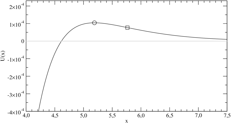
Figure 1: Scalar field potential $U(x):=V(x)/(M_{P}^{2}\sqrt{\tilde{\beta}_{\odot}})$ from Eq. (28) with $x=\sqrt{\frac{2}{3}}\varphi/M_{P}$. Here, $x_{s}$ was chosen such that $U(0)=-\frac{3}{4}e^{x_{s}/2}=-10$. The circle is at the maximum and the square at the inflection point of $U(x)$. To the right of the latter the scalar mass squared is positive. Note that both limits $U(x\rightarrow 0)$ and $U(x\rightarrow\infty)\rightarrow 0$ are valid only for the pure $\beta_{\odot}/R$ model since the effects of the $\beta/B$ term will be important there.

Thus, within the same approximation,

$$V^{\prime}(\varphi)=-\sqrt{\frac{3}{2}}M_{P}\sqrt{\tilde{\beta}_{\odot}}\left(e^{\frac{x}{2}}-e^{\frac{x_{s}}{2}}\right)e^{-2x},\ \ \ V^{\prime\prime}(\varphi)=2\sqrt{\tilde{\beta}_{\odot}}\left(\frac{3}{4}e^{\frac{x}{2}}-e^{\frac{x_{s}}{2}}\right)e^{-2x}.$$ (29)

Exactly at the SdS solution $x=x_{s}$ we obtain $V^{\prime}(\varphi_{s})=0$ and $V^{\prime\prime}(\varphi_{s})=-6r_{e}^{-2}/e^{x_{s}}<0$, indicating that the SdS solution is actually a maximum, see Fig. 1. Noting that a scalar mass term in the Einstein frame transforms as $\sqrt{|\tilde{g}|}\,m_{\varphi}^{2}\,\varphi^{2}\to(F^{\prime})^{2}\sqrt{|{g}|}\ m_{\varphi}^{2}\,(\varphi^{2}/F^{\prime})=\sqrt{|{g}|}\ (F^{\prime}\,m_{\varphi}^{2})\,\varphi^{2}$ into the Jordan frame, it follows that the mass squared of $\varphi$ in the Jordan’s frame is, in our case, $m_{\varphi,J}^{2}=-6r_{e}^{-2}$. The fact that it is negative is not a surprise, it was expected from the aforementioned fact that at the cosmological level the de Sitter solution is a maximum and hence unstable [14], its lifetime being of order $H_{0}^{-1}$. However, when $e^{x/2}$ moves to larger values than $\frac{4}{3}e^{x_{s}/2}$, then $m_{\varphi,J}^{2}$ becomes positive and acquires physical meaning. From then on the scalar field $\varphi$ behaves like decaying quintessence. At the inflection point the vacuum energy $V(e^{x/2}=\frac{4}{3}e^{x_{s}/2})=({189}/{256})\,V(\varphi_{s})$ is of the same order of magnitude as the de Sitter cosmological constant. Thus the relaxation mechanism works also in the stable quintessence regime.

It is interesting to reconfirm the above Jordan’s frame calculation of the mass squared of the new gravitational d.o.f. by expanding around the constant background Ricci scalar $R_{0}=12r_{e}^{-2}$. Following the general procedure of [29, 30], we obtain the vacuum Klein-Gordon equation in the Jordan frame, namely $\left(\Box+m_{R_{1}}^{2}\right)\,R_{1}=0$, where the gravitational d.o.f. is denoted now by $R_{1}(r)$, and $m_{R_{1}}^{2}$ its mass squared:

$$m_{R_{1}}^{2}=\frac{\left[F^{\prime}(R_{0})-R_{0}F^{\prime\prime}(R_{0})-3\square F^{\prime\prime}(R_{0})\right]}{3F^{\prime\prime}(R_{0})}=-\frac{1}{2}R_{0}=-6r_{e}^{-2},$$ (30)

and we used $F(R)=-{\tilde{\beta}_{\odot}}/{R}$, $F^{\prime}(R)={\tilde{\beta}_{\odot}}/{R^{2}}$, $F^{\prime\prime}(R)=-{2\tilde{\beta}_{\odot}}/{R^{3}}$. We note that $m_{R_{1}}^{2}$ exactly coincides with $m_{\varphi,J}^{2}$, which confirms our expectations. From this alternative approach, we most clearly see that the large value of $\tilde{\beta}_{\odot}\propto\rho_{\Lambda}^{i}$ does not enter the mass calculation, which means that the result does not depend neither on the size nor on the sign of $\rho_{\Lambda}^{i}$. This is different from the previously considered $\mu^{4}/R$ or $R^{2}/\mu^{2}$ models in the literature [23, 24, 25, 26, 27, 28, 29, 30], where the mass is directly related to the parameter $\mu$.

3.4 Coupling to matter

Let us consider first the influence of matter on the evolution of $\varphi$, and leave for the next section the study of the role of $\varphi$ in the field equation of matter. The corresponding Einstein’s frame action reads

$$S=\int d^{4}x\sqrt{|\tilde{g}|}\left[\frac{1}{2}M_{P}^{2}\tilde{R}+\frac{1}{2}\tilde{g}^{ab}\,\partial_{a}\varphi\,\partial_{b}\varphi-V(\varphi)+\frac{1}{\sqrt{|\tilde{g}|}}\mathcal{L}_{\text{mat}}[g_{ab}]\right]\,,$$ (31)

where $g_{ab}=\tilde{g}_{ab}/(F^{\prime})$ is the $\varphi$-dependent Jordan frame metric, and $\mathcal{L}_{\text{mat}}$ is the matter Lagrangian density still in the original Jordan’s frame variables and containing the density factor $\sqrt{|g_{ab}|}$ in the Jordan metric. First, we look at the Einstein equations following from $2\delta S/\delta\tilde{g}_{ab}=0$,

$$M_{P}^{2}\tilde{G}^{ab}+\tilde{T}_{\varphi}^{ab}+\frac{2}{\sqrt{|\tilde{g}|}}\frac{\delta\mathcal{L}_{\text{mat}}[g_{ab}]}{\delta\tilde{g}_{ab}}=0,$$ (32)

where $\tilde{T}_{\varphi}^{ab}$ is the standard energy-momentum tensor of the canonically normalized scalar field including  $V(\varphi)$. The matter energy-momentum tensor reads

$$\tilde{T}_{\text{mat}}^{ab}=\frac{2}{\sqrt{|\tilde{g}|}}\frac{\delta\mathcal{L}_{\text{mat}}[g_{ab}]}{\delta\tilde{g}_{ab}}=\frac{2}{\sqrt{|\tilde{g}|}}\frac{\delta\mathcal{L}_{\text{mat}}[g_{ab}]}{\delta g_{ab}}\frac{\partial g_{ab}}{\partial\tilde{g}_{ab}}=\frac{2}{\sqrt{|\tilde{g}|}}\frac{\delta\mathcal{L}_{\text{mat}}[g_{ab}]}{\delta g_{ab}}\frac{1}{F^{\prime}},$$ (33)

which depends on $\varphi$, too. Next we discuss the equations of motion for $\varphi$, given by

$$\frac{\delta S}{\delta\varphi}=-\tilde{\square}\varphi-V^{\prime}(\varphi)+\frac{1}{\sqrt{|\tilde{g}|}}\frac{\delta\mathcal{L}_{\text{mat}}}{\delta\varphi}=0,$$ (34)

where the variational derivative in the last term can be determined with the help of Eq. (33),

$$\frac{\delta\mathcal{L}_{\text{mat}}[g_{ab}]}{\delta\varphi}=\frac{\delta\mathcal{L}_{\text{mat}}[g_{ab}]}{\delta g_{ab}}\frac{\partial g_{ab}}{\partial\varphi}=\frac{\sqrt{|\tilde{g}|}}{2}F^{\prime}\tilde{T}_{\text{mat}}^{ab}\tilde{g}_{ab}\frac{\partial F^{\prime}}{\partial\varphi}\frac{-1}{(F^{\prime})^{2}}=-\frac{\sqrt{|\tilde{g}|}}{\sqrt{6}\,M_{P}}\,\tilde{T}_{\text{mat}}^{ab}\tilde{g}_{ab}\,,$$ (35)

and in the last equality we used (25). Thus Eq. (34) can be cast as $\tilde{\square}\varphi+V^{\prime}(\varphi)+\tilde{T}_{\text{mat}}^{ab}\tilde{g}_{ab}/\left(\sqrt{6}M_{P}\right)=0$, where $\varphi$ is seen to couple to the trace of $\tilde{T}_{\text{mat}}^{ab}$. The relation with the corresponding energy-momentum tensor in the Jordan frame follows from (33): $\tilde{T}_{\text{mat}}^{ab}=\sqrt{|{g}|/|\tilde{g}|}\,{T}_{\text{mat}}^{ab}/F^{\prime}=\left(F^{\prime}\right)^{-3}\,{T}_{\text{mat}}^{ab}$, and hence the traces in both frames are related by $\ \tilde{g}_{ab}\tilde{T}_{\text{mat}}^{ab}=\left(F^{\prime}\right)^{-2}\,g_{ab}\,{T}_{\text{mat}}^{ab}$. Finally, since ${T}_{\text{mat}}^{ab}g_{ab}=\rho_{\text{mat}}$ provides the physical (non-relativistic) matter density in the Jordan frame, we arrive at the effective field equation for $\varphi$:

$$\tilde{\square}\varphi+V^{\prime}(\varphi)+\frac{1}{\sqrt{6}}\,\left(\frac{\rho_{\text{mat}}}{M_{P}\,{F^{\prime}}^{2}}\right)=0\,.$$ (36)

We may now compare the two source terms driving the evolution of $\varphi$, viz. $V^{\prime}(\varphi)$ and $\rho_{\text{mat}}/(M_{P}{F^{\prime}}^{2})$. If we look at the beginning of the quintessence regime ($\varphi\gtrsim\varphi_{s}$), where $\rho_{\text{mat}}\sim\rho_{c}^{0}=3M_{P}^{2}r_{e}^{-2}$, the first source is of order $V^{\prime}(\varphi)\sim(M_{P}\,r_{e}^{-2})/F^{\prime}\sim\rho_{c}^{0}/(M_{P}\,F^{\prime})$, whereas the second source is of order $\sim\rho_{c}^{0}/(M_{P}{F^{\prime}}^{2})$ and hence much smaller owing to the additional suppression factor of $F^{\prime}$. This shows that the evolution of $\varphi$ is dominated by $V(\varphi)$. Hence, matter does not disturb the relaxation mechanism. This is not surprising because it is related to the dominance of the curvature by the relaxation mechanism. Indeed, if we take the trace of Eq. (32), we obtain $M_{P}^{2}\tilde{R}=\tilde{T}_{\varphi}^{ab}\tilde{g}_{ab}+\tilde{T}_{\text{mat}}^{ab}\tilde{g}_{ab}$. From (27) we see that the first term on the righthand side of the trace is of the order $V(\varphi_{s})\sim\rho_{c}^{0}\,(F^{\prime})^{-1}$ during the slow-roll regime, whereas the second term is $\sim\rho_{c}^{0}\,(F^{\prime})^{-2}$, which is once more smaller than $V(\varphi_{s})$ by a factor of $(F^{\prime})^{-1}$.

3.5 Possible fifth forces with matter

In the previous section we found that the evolution of the gravitational scalar $\varphi$ is not disturbed by matter. Conversely, now we wish to study if matter can be significantly affected by the presence of $\varphi$. We will illustrate it by considering the effect on a matter scalar field $\psi$ with mass $m_{\psi}$ in the Jordan frame. The corresponding matter action reads

$$S_{\text{mat}}[g_{ab},\psi]=\int d^{4}x\sqrt{|g|}\left[\frac{1}{2}g^{ab}\,\partial_{a}\psi\,\partial_{b}\psi-\frac{1}{2}m_{\psi}^{2}\psi^{2}\right].$$ (37)

From the conformal transformation (23), and the associated relation $g^{ab}=(F^{\prime})\,\tilde{g}^{ab}$, we switch into the Einstein frame. The complete action in this frame is given in Eq. (26), where in the present case the matter part reads

$$\tilde{S}_{\text{mat}}\equiv S_{\text{mat}}\left[\frac{\tilde{g}_{ab}}{F^{\prime}}\right]=\int d^{4}x\sqrt{|\tilde{g}|}\left[\frac{1}{F^{\prime}}\,\frac{1}{2}\tilde{g}^{ab}\,\partial_{a}\psi\,\partial_{b}\psi-\frac{1}{(F^{\prime})^{2}}\,\frac{1}{2}m_{\psi}^{2}\psi^{2}\right]\,.$$ (38)

The equation of motion for the matter scalar field $\psi$ follows as usual from the variational principle $\delta\tilde{S}_{\text{mat}}/\delta\psi=0$. After some standard manipulations and partial integration, we arrive at

$$\delta{\tilde{S}}_{\text{mat}}=-\int d^{4}x\sqrt{|\tilde{g}|}\left[\frac{1}{\sqrt{|\tilde{g}|}}\partial_{a}\left(\frac{1}{F^{\prime}}\,\sqrt{|\tilde{g}|}\,\tilde{g}^{ab}\,\partial_{b}\psi\,\right)+\frac{m_{\psi}^{2}}{(F^{\prime})^{2}}\,\psi\right]\,\delta\psi.$$ (39)

The first term in the bracket at the integrand can be written as

$$\frac{1}{F^{\prime}}\,\frac{\partial_{a}\left(\sqrt{|\tilde{g}|}\,\tilde{g}^{ab}\,\partial_{b}\psi\right)}{\sqrt{|\tilde{g}|}}+\tilde{g}^{ab}\,\partial_{b}\psi\,\partial_{a}\left(\frac{1}{F^{\prime}}\right)=\frac{1}{F^{\prime}}\,\tilde{\square}\psi-\frac{\tilde{g}^{ab}\,\partial_{b}\psi}{(F^{\prime})^{2}}\,\frac{\partial F^{\prime}}{\partial\varphi}\,\partial_{a}\varphi\,,$$ (40)

and then using (25) we finally obtain the full equation of motion for the matter scalar $\psi$:

$$\tilde{\square}\psi-\tilde{g}^{ab}(\partial_{b}\psi)\sqrt{\frac{2}{3}}\frac{\partial_{a}\varphi}{M_{P}}+\frac{1}{F^{\prime}}\,m_{\psi}^{2}\psi=0.$$ (41)

When the gravitational scalar $\varphi$ is in a slow-roll regime we have $|\partial_{a}\varphi|\lesssim\sqrt{2\,V(\varphi_{s})}=\sqrt{6}\,M_{P}\,r_{e}^{-1}/\sqrt{F^{\prime}}$, where $V(\varphi_{s})$ was given in (27). The maximal coupling with matter appears when $\partial_{a}\varphi$ saturates the slow roll bound, in which case the equation of motion for $\psi$ in the Einstein frame can be cast in a simplified notation as follows:

$$\tilde{\square}\psi-2\,\frac{r_{e}^{-1}}{\sqrt{F^{\prime}(\varphi)}}\,(\partial\psi)+\frac{m_{\psi}^{2}}{F^{\prime}(\varphi)}\psi=0\,.$$ (42)

Here, the mass $m_{\psi,E}=m_{\psi}/\sqrt{F^{\prime}}$ corresponds to that of the matter field $\psi$ in the Einstein frame and contains the factor $\sqrt{F^{\prime}}$. We see from (42) that this factor is shared by the fifth force “friction” coupling of matter ($\psi$) with $\varphi$ in that frame: $\Gamma_{\psi,E}\sim r_{e}^{-1}/\sqrt{F^{\prime}(\varphi)}$. Since the dimensionless ratio $\Gamma_{\psi,E}/m_{\psi,E}=r_{e}^{-1}/m_{\psi}$ is independent of $F^{\prime}$, the relative strength of the fifth force acting on the matter field $\psi$ (measured by comparing it to its mass) is the same for all frames. Thus, we find $\Gamma_{\psi,J}=\left(\Gamma_{\psi,E}/m_{\psi,E}\right)\,m_{\psi}=r_{e}^{-1}$ for the effective fifth force strength in the Jordan frame. In other words, this coupling is essentially given by the present Hubble rate: $r_{e}^{-1}\approx H_{0}$. Even in the considered case, where the coupling of $\varphi$ to matter is maximal, we obtained an extremely weak fifth force. Therefore, we must conclude that such coupling is completely unobservable. It is also interesting to mention the effect of $\varphi$ on photon interactions with matter. Since the action for photons is invariant under conformal transformations of the metric, they are not subject to explicit fifth forces mediated by $\varphi$. However, they feel the metric deviation in our modified gravity model with respect to standard General Relativity. This effect might be detected by gravitational lensing experiments depending on the strength of the deviation. We briefly address this possibility in the next section.

4 Numerical results for the large scale astrophysical domain

The large scale cosmological domain characterized by the FLRW metric was studied in detail in [14, 15], and we saw it is dominated by the $\beta/B$ term in (1). We have argued in Sec. 2 that the $\beta/B$ term in the action is also the dominant term at large length scales for the metric (7), which is more in accordance with the astrophysical environment. Unfortunately, due to the occurrence of the Gauß-Bonnet invariant in (4) it is difficult to find exact solutions on a spherically symmetric background. This is quite obvious from the complicated structure of the field equations (2)-(3), especially when the curvature invariants are non-constant. We will show here some numerical solutions of these equations in the vacuum case and we briefly discuss the deviation from the standard SdS solution. The latter metric, as given by equations (7) and (11), will be used for setting the initial conditions for large radius $r$, i.e. the situation for which the $\beta$-terms dominate over the $\beta_{\odot}$ ones. This procedure ensures a smooth transition to the cosmological de Sitter result.

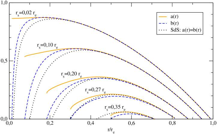
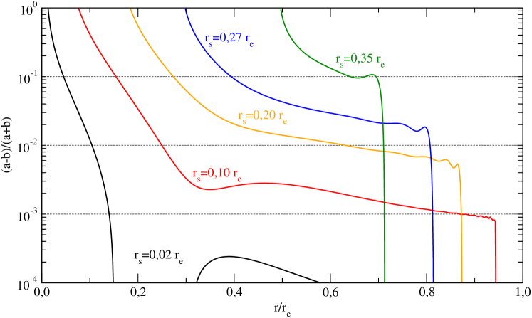
Figure 2: Top: numerical solutions for the functions $a(r)$ and $b(r)$ in the spherically symmetric metric (7) for the pure $\beta/B$ model without matter. The initial conditions have been fixed close to the higher zero of the corresponding SdS solution (11), which is plotted, too. Bottom: relative differences $\frac{a(r)-b(r)}{a(r)+b(r)}$ of the numerical functions $a(r)$ and $b(r)$. Note that the numerical error dominates around the higher zeros of both functions.

Specifically, to obtain the pure effects of the $\beta/B$ term, we set $\beta_{\odot}$ to zero in (3), and the initial conditions for the metric are set very close but below the higher zero of the function $a(r)$ in Eq. (11). For small values of the Schwarzschild radius parameter $r_{s}\ll r_{e}$ this is approximately at $r=r_{e}$. As we know already, $r_{s}=0$ corresponds to the de Sitter solution, which is exact also for the $\beta/B$ model. Therefore, we consider only solutions with non-zero $r_{s}$. Some examples are shown in Fig. 2, where the two functions $a(r)$ and $b(r)$ in the metric (7) are displayed together with the standard SdS result. Let us note that in the case of small perturbations, one usually writes $a(r)=1+2\Psi(r)$ and $b(r)=1+2\,\Phi(r)$ where $\Psi(r)$ and $\Phi(r)$ are the two gravitational potentials associated to the metric. While in the standard SdS case they are equal, in the present case we look for deviations $a(r)-b(r)=2[\Psi(r)-\Phi(r)]$ that could provide information of the modified gravity model. As expected, these deviations grow with increasing $r_{s}$. While $b(r)$ follows qualitatively the standard result, the function $a(r)$ stays at larger values especially for small $r$, which we identify as an effect of the $r$-dependence in $B$. The relative difference between both metric functions is plotted also in Fig. 2 (bottom), it is of order one around the lower zero of $b(r)$. However, we expect that this singular point must lie within the matter distribution, whose metric has to be matched to the vacuum solution in Fig. 2 at a larger radius $r$. Whether this matching is possible and how the inner solution for the metric behaves, depends strongly on the properties of the matter distribution. We keep this question open for a future investigation. At the moment we cannot exclude the possibility that at intermediate (intergalactic) scales some non-trivial corrections to standard expectations might creep in. We provide some discussion of this possibility in the next section.

5 Possible gravity modifications at large distances

Let us return for a moment to the discussions made in Sect. 2. We have seen that while both at local astrophysical scales and at very large cosmological domains the relaxation mechanism works perfectly well and can be studied analytically, at intermediate scales our knowledge is more limited and we need to resort to the numerical analysis within some approximations, as we have seen in the previous section. The characteristic distance entering the potential deviations is

$$r_{c}\sim\left(r_{s}^{2}r_{e}^{2}\frac{\beta_{\odot}}{\beta}\right)^{1/6}\,,$$ (43)

where we know that $\beta$ and $\beta_{\odot}$ are fixed in order of magnitude and (same) sign by the condition that the relaxation mechanism works in the cosmological and astrophysical domains, respectively. These conditions entail the relations $|\beta|\sim\rho_{\Lambda}^{i}\,H_{0}^{4}$ and $|\beta_{\odot}|\sim\rho_{\Lambda}^{i}\,H_{0}^{2}$. Hence it follows from (43) that

$$r_{c}\sim\left(\frac{r_{s}^{2}r_{e}^{2}}{H_{0}^{2}}\right)^{1/6}\sim\left(\frac{r_{s}}{H_{0}^{2}}\right)^{1/3}=\left(\frac{G_{N}\,M_{s}}{H_{0}^{2}}\right)^{1/3}\,,$$ (44)

where $M_{s}$ is the mass of the galaxy or cluster of galaxies sourcing the gravitational field. We may compare this length scale with the one at which one expects deviations to the Newtonian gravity at large distances in ordinary extended gravity theories, i.e. with a late-time modification of the gravitational interaction [19, 20, 21, 22, 23, 24, 25, 26]. These effects have been specifically addressed in Ref.  [31] by considering a Lagrangian modification of the form $\delta{\cal L}=M_{P}^{2}\,\mu^{4n+2}/Q^{n}$ with $Q=R^{abcd}R_{abcd}$ the square Riemann tensor. For $n=1$ this is not far away from the behavior of the gravity modification in our relaxation model (1) at large distances, except that in our case we have both a gravity modification and the large CC in mutual interplay. It is however illustrative to compare the two kind of models for $n=1$ , for which the the characteristic scale of the induced modification of Newtonian gravity is

$$r_{c}^{*}\sim\left(\frac{\left(G_{N}\,M_{s}\right)^{2}}{H_{0}^{3}}\right)^{1/5}\,,$$ (45)

after setting $\mu\sim H_{0}$, which is the extremely small value that is necessary to choose for the $\mu$-parameter in order to explain the late-time cosmic acceleration in this kind of models  [31]. The ratio between the two characteristic length scales is

$$\frac{r_{c}^{*}}{r_{c}}\sim\left(G_{N}M_{s}\,H_{0}\right)^{1/15}={\cal O}(0.1)\,.$$ (46)

For the numerical evaluation of this ratio we have used the source mass of a relatively large galaxy (say, $M_{s}\sim 10^{11}\,M_{\odot}$, i.e. with a number of solar masses similar to our galaxy), or the mass of a large cluster of similar galaxies. In both cases the two length scales do not differ in more than one order of magnitude, so they are indeed very close. In other words, in both classes of models (relaxation model and ordinary late-time extended gravity) we expect deviations from Newtonian gravity at similar large scales in the $100$ kpc-Mpc range, as it follows from the above formulae. Let us remark, however, that in the relaxation model we have a double bonus which is absent in the ordinary case, to wit: i) we do not need to use extremely small scales as $\mu\sim H_{0}\sim 10^{-33}$ eV but rather scales ${\cal M}\sim$ meV and ${\cal M}^{\prime}\sim$ MeV both lying in the natural SM range (cf. Sect. 2); and ii) the local astrophysical domain is protected from unwanted vacuum effects even in the presence of the large $\rho_{\Lambda}^{i}$. Indeed, the typical value of $r_{c}$ emerging from (44) is roughly from $10$ to $100$ kpc in the case of a galaxy, whereas for a large cluster it may reach the few Mpc level. As these length scales are at the same time the characteristic sizes of a galaxy and a cluster of galaxies, respectively, it follows that the local astrophysical domains remain well protected from large vacuum effects in our relaxation models. Finally, in the intermediate region beyond these distances (say up to $\sim 10-100$ Mpc) we cannot study the problem in a simple way, as the numerical analysis of the previous section has shown, because the SdS metric is no longer a good approximate solution. Only after attaining very large distances (of order of a few hundred Mpc at least) we retrieve again the relaxation mechanism in the cosmological domain [14] with all its phenomenological success [15].

6 Conclusions

In this letter, we have performed a first investigation of the modified gravity implementation of the CC relaxation mechanism in a static and spherically symmetric background, which serves as an approximation for the study of the mechanism at length scales characteristic of the astrophysical domain. We found the mechanism to be working in the sense that the space-time curvature is not dominated by the initial large vacuum energy density $\rho_{\Lambda}^{i}$. Instead, a small effective dark energy density $\mathcal{O}(M_{P}^{2}r_{e}^{-2})\sim M_{P}^{2}\,H_{0}^{2}\sim\rho_{\Lambda}^{0}$ is found, similar to our earlier results in a cosmological background [14]. Moreover, we studied the influence of fifth forces on massive objects, which turned out to be long ranged, but extremely weak and therefore inconspicuous. This shows that the idea of CC relaxation may be useful in more general contexts than just in cosmology. Given the unconventional starting point, one could not naively expect this local astrophysical behavior from the beginning. Interestingly, we also found that at very large scales of order of $10^{-2}\,H_{0}^{-1}$ the metric may deviate significantly from the standard SdS solution, thus opening up a possible way to detect this mechanism via gravitational lensing and other effects.

Possible observable implications at these scales have already been proposed in other modified gravity theories [31]. In the light of these studies one can foresee deviations from the standard Newtonian/GR behavior at length scales of $100$ kpc-Mpc. We cannot exclude, for instance, the possible implications of these deviations e.g. by changing the required abundances of dark matter in the intergalactic domains in order to explain the DM problem in the large. However, the investigation of these potentially relevant issues goes far beyond the content of the present Letter. Their more precise description is therefore an important future challenge in the CC relaxation approach.

Finally, some theoretical issues remain open for further study; in particular, the fact that the relaxation mechanism exerts such a dominating influence. In this sense, further insight should go into the direction of finding ways to complete this model and understanding the role of the vacuum energy versus the matter sources. Quite in contrast to the present approach, the usual modifications of gravity disclaim ab initio any understanding of how to cope with the huge vacuum energy injected in the universe by QFT/string theory, and just focus on late-time simulations of the measured effect. This way is therefore no more satisfactory. A link between the two points of view is still missing, and hence more work is required to understand the ultimate interplay between gravitation, vacuum energy and matter in our cosmos. We hope that our approach may offer a new perspective for an eventual solution of this difficult problem.

Acknowledgments

FB and JS would like to thank D. Polarski for very useful discussions. The authors have been partially supported by DIUE/CUR Generalitat de Catalunya under project 2009SGR502; FB and JS also by MEC and FEDER under project FPA2007-66665 and by the Consolider-Ingenio 2010 program CPAN CSD2007-00042, and HS also by the Ministry of Education, Science and Sports of the Republic of Croatia under contract No. 098-0982930-2864.

References

- [1] S. Weinberg, Rev. Mod. Phys. 61 (1989) 1.
- [2] E. Komatsu et al. Astrophys. J. Suppl. 192 (2011) 18, arXiv:1001.4538.
- [3] R. Knop et al., Astrophys. J. 598 (2003) 102.
- [4] A. Riess et al., Astrophys. J. 607 (2004) 665.
- [5] P.J.E. Peebles and B. Ratra, Rev. Mod. Phys. 75 (2003) 559.
- [6] T. Padmanabhan, Phys. Rep. 380 (2003) 235.
- [7] V. Sahni, A. Starobinsky, Int. J. of Mod. Phys. A9 (2000) 373.
- [8] S.M. Carroll, Living Rev. Rel. 4 (2001) 1.
- [9] E.J. Copeland, M. Sami, S. Tsujikawa, Int. J. of Mod. Phys. D15 (2006) 1753.
- [10] M. Li , X-D. Li, S. Wang, Y. Wang, [arXiv:1103.5870].
- [11] F. Bauer, J. Solà, H. Štefančić, Phys. Lett. B688 (2010) 269 [arXiv:0912.0677].
- [12] F. Bauer, J. Solà, H. Štefančić, Phys. Lett. B678 (2009) 427 [arXiv:0902.2215].
- [13] H. Štefančić, Phys. Lett. B670 (2009) 246 [arXiv:0807.3692].
- [14] F. Bauer, J. Solà, H. Štefančić, JCAP 1012 (2010) 030 [arXiv:1006.3944].
- [15] S. Basilakos, F. Bauer, and J. Solà, Confronting the relaxation mechanism for a large cosmological constant with observations [arXiv:1109.4739].
- [16] S. Finazzi, S. Liberati and L. Sindoni, arXiv:1103.4841.
- [17] M. Maggiore, Phys. Rev. D83 (2011) 063514 [arXiv:1004.1782].
- [18] G. Mangano, Phys. Rev. D82 (2010) 043519 [arXiv:1005.2758].
- [19] S. Nojiri, S.D. Odintsov, Phys. Rev. D68 (2003) 123512 [hep-th/0307288].
- [20] S. Capozziello, S. Carloni and A. Troisi, Recent Res. Dev. Astron. Astrophys. 1 (2003) 625 [astro-ph/0303041].
- [21] S.M. Carroll, V. Duvvuri, M. Trodden, M.S. Turner, Phys. Rev. D70 (2004) 043528 [astro-ph/0306438].
- [22] S.M. Carroll, A. de Felice, V. Duvvuri, D.A. Easson, M. Trodden, M.S. Turner, Phys. Rev. D71 (2005) 063513 [astro-ph/0410031].
- [23] S. Nojiri and S.D. Odintsov, Int. J. Geom. Meth. Mod. Phys. 4 (2007) 115 [hep-th/0601213].
- [24] T.P. Sotiriou, V. Faraoni, Rev. Mod. Phys. 82 (2010) 451 [arXiv:0805.1726].
- [25] R. Woodard, Lect. Notes Phys. 720 (2007) 403 [arXiv.astro-ph/0601672].
- [26] S. Capozziello, M. De Laurentis, [arXiv:1108.6266].
- [27] L. Amendola, R. Gannouji, D. Polarski, S. Tsujikawa, Phys. Rev. D75 (2007) 083504 [arXiv:gr-qc/0612180].
- [28] S. A. Appleby, R. A. Battye, A. A. Starobinsky, JCAP 06 (2010) 005 [arXiv:0909.1737].
- [29] T. Chiba, T. L. Smith and A. L. Erickcek, Phys. Rev. D 75 (2007) 124014 [arXiv:astro-ph/0611867].
- [30] T. Chiba, Phys. Lett. B 575 (2003) 1 [arXiv:astro-ph/0307338].
- [31] I. Navarro, K. Van Acoleyen, Phys. Lett. B622 (2005) 1 [arXiv:gr-qc/0506096].