Newtonian Perturbations on Models with Matter Creation

Abstract

Creation of Cold Dark Matter (CCDM) can macroscopically be described by a negative pressure, and, therefore, the mechanism is capable to accelerate the Universe, without the need of an additional dark energy component. In this framework we discuss the evolution of perturbations by considering a Neo-Newtonian approach where, unlike in the standard Newtonian cosmology, the fluid pressure is taken into account even in the homogeneous and isotropic background equations (Lima, Zanchin and Brandenberger, MNRAS 291, L1, 1997). The evolution of the density contrast is calculated in the linear approximation and compared to the one predicted by the $\Lambda$CDM model. The difference between the CCDM and $\Lambda$CDM predictions at the perturbative level is quantified by using three different statistical methods, namely: a simple $\chi^{2}$-analysis in the relevant space parameter, a Bayesian statistical inference, and, finally, a Kolmogorov-Smirnov test. We find that under certain circumstances the CCDM scenario analyzed here predicts an overall dynamics (including Hubble flow and matter fluctuation field) which fully recovers that of the traditional cosmic concordance model. Our basic conclusion is that such a reduction of the dark sector provides a viable alternative description to the accelerating $\Lambda$CDM cosmology.

I Introduction

The growing evidences for cosmic acceleration as, e.g., the Supernova Ia observations riess98 ; Ko2008 ; Hi2009 ; Aman2010 , is challenging cosmologists and theoretical physicists. The neediness of some new ingredient in the cosmic recipe, in order to preserve Einstein’s Equations, inspired both communities to conservatively invoking the simplest available hypothesis, namely, a cosmological constant, $\Lambda$.

Nevertheless, the identification of $\Lambda$ with the quantum vacuum has brought another problem: the estimate of theoretical physicists that the vacuum energy density should be 120 orders of magnitude bigger than the measured $\Lambda$ value. This is the “old” cosmological constant problem (CCP) weinb89 . The “new” problem Peebles03 asks why is the vacuum density so similar to the matter density just now? Many solutions to both problems have been proposed in the literature Zlatev99 ; AASW09 . The majority of them are plagued with no physical basis and/or many parameters.

On the other hand, some authors have also investigated a class of models where the creation of cold dark matter may result on a pressure which is negative (named CCDM, Creation of Cold Dark Matter), thereby providing a mechanism for cosmic acceleration. In the current literature, the leitmotiv of such models is to reduce the dark sector (dark energy + dark matter) in the framework of general relativity since the existence of dark energy seems to be less secure than dark matter BDRS03 ; PDM . The extra bonus is to solve the coincidence and cosmological constant problems.

The search for dark matter accelerating models started almost one decade before the SNe Ia observations. Initially, Prigogine and coworkers Pri89 argued that the gravitationally-induced particle creation could consistently be discussed in the realm of the relativistic non-equilibrium thermodynamics. Later on, their macroscopic formulation was clarified by Calvão, Lima and Waga through a manifestly covariant formulation CLW92 . The inclusion of the back reaction in the Einstein Field Equations (EFE) via an effective pressure (which is negative for an expanding space-time) opened the way for cosmological applications. As a consequence, several interesting features of cosmologies where the dark sector is reduced due to the creation of CDM matter have been discussed in the last decade LSS08 ; SSL09 .

More recently, a new CCDM cosmology was proposed by Lima, Jesus and Oliveira (from now on LJO model) which mimics the Hubble expansion history of the $\Lambda$CDM model, at least at the level of the background equations LJO .

The quoted LJO model is quite interesting, once that it perfectly mimics the $\Lambda$CDM cosmic history, thereby also providing a good fit to current cosmological data (SNIa, BAO and CMB shift parameter, total age, etc) with the same number of parameters of the $\Lambda$CDM, but without the CCP. In this sort of models, the quantum vacuum energy is canceled out by some not yet known physical mechanism. A basic advantage of this kind of scenario comes from the fact that a vacuum energy density which is null or negligible is more acceptable than a vacuum energy density finely tuned like in the $\Lambda$CDM model.

Naturally, although providing good fits to background data, it would be interesting to investigate to which level this similarity is preserved, for instance, by analyzing the evolution of small fluctuations predicted by the CCDM equations. Preliminary studies on this subject has already been accomplished by Basilakos and Lima BasLim , however, focusing on the theoretical consequences to cluster abundances at different redshifts (see also BPL2010 ). By using the Press-Schechter formalism, they also investigated the cluster-size halo redshift distribution by confronting the results with future cluster surveys (eROSITA satellite and Sunayev-Zeldovich survey based on the South Pole Telescope). We would like to stress that in the latter papers we ignored possible contributions from pressure at the perturbative level.

In the present paper, we are basically interested to determine whether the LJO model provides a realistic description at the perturbative level, however, by fitting the available fluctuation data, like the growth rate of clustering. The difference between the CCDM and $\Lambda$CDM predictions at the perturbative level is quantified using tree different statistical methods, namely: a simple $\chi^{2}$-analysis in the relevant space parameter, a Bayesian statistical inference, and, finally, a Kolmogorov-Smirnov test. As we shall see, the CCDM reduction dark sector provides a viable alternative description to the accelerating $\Lambda$CDM cosmology.

The work is planned as follows. The general relativistic approach for CCDM models is presented in section II. In sections III we show how the Neo-Newtonian treatment adopted here recovers the relativistic formulation whereas, in section IV, we derive the associated evolution equation for the density contrast. In section V, we discuss in detail the linear growth factor of matter perturbations, the CCDM theoretical predictions regarding the evolution of the growth rate of clustering, and the corresponding statistical analyzes. The main conclusions are summarized in VI.

II CCDM Cosmology in the matter era: Relativistic Formulation

The background cosmological equations of the model with creation of cold dark matter (CCDM) have the following form (for simplicity, we are neglecting the contributions of the radiation and baryonic components):

$$8\pi G\rho = 3\frac{\dot{a}^{2}}{a^{2}}+3\frac{K}{a^{2}},$$ (1)

$$8\pi Gp_{c} = -2\frac{\ddot{a}}{a}-\frac{\dot{a}^{2}}{a^{2}}-\frac{K}{a^{2}}.$$ (2)

where $\rho$ is the CDM density, $p_{c}$ is the creation pressure, $a(t)$ is the scale factor, and an overdot means time derivative. In the case of constant specific entropy (per particle), the creation pressure for a CDM component is given by Pri89 ; CLW92

$$p_{c}=-\frac{\rho\Gamma}{3H},$$ (3)

where $\Gamma$ is the creation rate of CDM particles and $H=\dot{a}/a$ is the Hubble parameter.

It is readily checked that equations (1) and (2) lead to the continuity and acceleration equations:

$$\frac{\dot{\rho}}{\rho}+3\frac{\dot{a}}{a} = \Gamma,$$ (4)

$$\frac{\ddot{a}}{a}=-\frac{4\pi G}{3}(\rho+3p_{c}) = -\frac{4\pi G\rho}{3}\left(1-\frac{\Gamma}{H}\right).$$ (5)

The above Eqs. (4-5) imply that the model is fully determined by the creation rate $\Gamma$, or more precisely, by the ratio $\Gamma/H$. If $\Gamma<<H$, the particle creation process is negligible, and the standard dust filled models are recovered. In the LJO scenario, the phenomenological creation rate of cold dark matter has been defined by:

$$\frac{\Gamma}{H}=3\tilde{\Omega}_{\Lambda}\frac{\rho_{c0}}{\rho},$$ (6)

where $\tilde{\Omega}_{\Lambda}$ (termed $\alpha$ in the original LJO notation LJO ) is a constant parameter, ${\rho_{c0}}$ is the present day value of the critical density, and the factor 3 has been added for mathematical convenience.

Now, by inserting the above expression into the energy conservation as given by (4) one obtains

$$\dot{\rho}+3H\rho=\Gamma\rho\equiv 3\tilde{\Omega}_{\Lambda}{\rho_{c0}}H,$$ (7)

which can be readily integrated to give a solution for the energy density

$$\rho=(\rho_{0}-\tilde{\Omega}_{\Lambda}\rho_{c0})a^{-3}+\tilde{\Omega}_{\Lambda}\rho_{c0}.$$ (8)

In terms of the cosmic history, the equivalence between this model and the $\Lambda$CDM model can be seen directly through the evolution equation of the scale factor function. As one may check, by inserting the expression of the creation pressure $p_{c}$ in Eq. (2) we obtain:

$$2a{\ddot{a}}+{\dot{a}}^{2}+K-3\tilde{\Omega}_{\Lambda}H_{0}^{2}a^{2}=0,$$ (9)

which should be compared to:

$$2a{\ddot{a}}+{\dot{a}}^{2}+K-{\Lambda}a^{2}=0,$$ (10)

provided by the $\Lambda$CDM model. The above equations imply that the models will have the same dynamical behavior when we identify the creation parameter by the expression $\tilde{\Omega}_{\Lambda}={\Lambda}/3{H_{0}}^{2}\equiv\Omega_{\Lambda}$. Further, the factor $\tilde{\Omega}_{m}\equiv\Omega_{m}-\tilde{\Omega}_{\Lambda}$, where $\Omega_{m}\equiv\frac{\rho_{0}}{\rho_{c0}}$, can also be identified as an ‘effective’ CDM density parameter, in comparison to the $\Lambda$CDM model LJO .

In the context of a spatially flat geometry ($K=0$ and $\Omega_{m}=1$), one may show that the inflection point, that is, the point where the Hubble expansion changes from the decelerating to the accelerating regime ($\ddot{a}(t_{I})=0$) takes place at:

$$a_{I}=\left[\frac{\tilde{\Omega}_{m}}{2\tilde{\Omega}_{\Lambda}}\right]^{1/3}\;.$$ (11)

As an example for $\tilde{\Omega}_{m}=1-\tilde{\Omega}_{\Lambda}=0.30$ we find $a_{I}\simeq 0.60$ (or $z_{I}\simeq 0.67$). Finally, the necessary condition for an inflection point in our past is $a_{I}<1$, which leads to the condition $\frac{1}{3}<\tilde{\Omega}_{\Lambda}<1$.

III Neo-Newtonian formulation for CCDM Cosmologies

The relativistic dynamics of CCDM cosmologies is the same of a single fluid with density $\rho$ and pressure $p_{c}$ (see Eqs. (1-3)). In addition, whether the equivalent fluid has an equation of state (hereafter EoS) parameter, $w=p/\rho$, taking a look at Eq. (3), we may see that this fluid ($p=p_{c}$), in general, has a time varying equation of state parameter, $w=-\frac{\Gamma}{3H}$.

In this connection, it is interesting to notice that fluids with non-vanishing pressure were also studied by Lima, Zanchin and Brandenberger lima97 within a ‘quasi’-Newtonian perspective. Following earlier ideas developed by McCrea MAC51 and Harrison H65 , they proposed the so called Neo-Newtonian description in order to reproduce the relativistic equations with pressure either at the background and perturbative levels. The basic equations of such a description are given by:

$$\left(\frac{\partial{\bf u}}{\partial t}\right)_{r}+({\bf u}\cdot\nabla_{r}){\bf u}=-\nabla_{r}\Phi-\frac{\nabla_{r}p_{c}}{\rho+p_{c}}$$ (12)

$$\left(\frac{\partial\rho}{\partial t}\right)_{r}+\nabla_{r}\cdot(\rho{\bf u})+p_{c}\nabla_{r}\cdot{\bf u}=0$$ (13)

$$\nabla_{r}^{2}\Phi=4\pi G(\rho+3p_{c})$$ (14)

where we have already included the creation pressure, $p_{c}$. These equations are named Euler, continuity and Poisson equations, respectively. The modified continuity equation is due to Lima et al. lima97 , in order to account correctly to pressure effects. As one may check, such equations reproduce the FRW type equations with pressure in the homogeneous and isotropic case ($p_{c}=p_{c}(t)$, $\rho=\rho(t)$), and can also be consistently perturbed for any given equation of state (see discussion below). In particular, they also shown that the linear perturbed version of these equations yield the correct growing mode for the density contrast of a fluid with $p=w\rho$, with constant $w$. For the case that $w$ is a time dependent quantity, the linear perturbation is equivalent to the full general relativistic formulation, at least when some conditions are imposed Reis2003 . Indeed, applications of this Neo-Newtonian approximation are not restricted to nonrelativistic matter, and the high accuracy of the approximation has also been proved for different epochs and even for scales larger than Hubble radius, as well as, for the spherical gravitational collapse Pad98 ; abramo07 . Therefore, it is reasonable to expect that the Neo-Newtonian approach will provide a good approximation for the evolution of small density fluctuations in the CCDM case.

III.1 Recovering the Relativistic CCDM Model from the Neo-Newtonian Approach

Let us now discuss how the basic relativistic equations of CCDM model can be recovered by the set of equations (12), (13), and (14). In order to show that, we first remark that homogeneity and spatial isotropy of the unperturbed model implies $\mathbf{u}=H\mathbf{r}$, according to the Hubble’s law. Then, Eq. (13) can be rewritten as:

$$\dot{\rho}+3H\rho=\Gamma\rho.$$ (15)

Assuming the creation rate $\Gamma$ as in the Eq.(6), the above equation can readily be integrated, to give exactly the same expression for the density evolution in Eq.(8). The Euler equation (12) can be rewritten as

$$\dot{H}{\bf r}+Hr\frac{\partial}{\partial r}(H{\bf r})=\left(\dot{H}+H^{2}\right){\bf r}=-{\bf\nabla}_{r}\Phi.$$ (16)

While the integration of the Poisson equation (14) yields:

$${\bf\nabla}_{r}\Phi=4\pi G(\rho+3p_{c})\frac{{\bf r}}{3},$$ (17)

Finally, by combining Eqs. (16) and (17), we derive the acceleration equation:

$$\frac{\ddot{a}}{a}=-\frac{4\pi G}{3}(\rho+3p_{c}),$$ (18)

where, as in the relativistic case, there is the presence of the creation pressure term, which can give rise for acceleration since it is negative for the expanding Universe. Using the expressions (3) and (8), the equation above can be integrated resulting in the following expression:

$$8\pi G\rho=3H^{2}+\frac{3K}{a^{2}}.$$ (19)

where $K$ is an arbitrary integration constant. This is Friedmann equation (1).

Thus, Eqs. (18) and (19) show that the background cosmological equations can effectively be recovered by the Neo-Newtonian formulation. This result is valid regardless of the specific form assumed to the creation rate $\Gamma$, and should be compared with the incomplete treatment adopted by Roany and Pacheco RP10 , and, critically, rediscussed by Lima et al. LJO2 .

IV Neo-Newtonian Density Perturbations

In general, a perturbative analysis in cosmology requires a full relativistic description since the standard non-relativistic (Newtonian) approach works well only when the scale of perturbation is much less than the Hubble radius and the velocity of peculiar motions are small in comparison to the Hubble flow peeb80 . However, as remarked earlier, such difficulties have been circumvented by the Neo-Newtonian approximation adopted here, and, therefore, such an approach may provide a good feeling about the behavior of the density perturbations.

To begin with, let us transform the Neo-Newtonian Equations (12)-(14) to comoving coordinates ${\bf x}$, which are related to the proper coordinates ${\bf r}$ by peeb93 ; lima97 :

$${\bf x}=\frac{{\bf r}}{a}.$$ (20)

In these coordinates, the basic quantities ${\bf u}$, $\rho$ and $\Phi$ can be rewritten as:

$${\bf u}=\dot{a}{\bf x}+a\dot{{\bf x}}=\dot{a}{\bf x}+{\bf v},$$ (21)

$$\rho=\bar{\rho}(t)[1+\delta({\bf x},t)],$$ (22)

$$p_{c}=\bar{p}_{c}(t)+\delta p_{c}({\bf x},t),$$ (23)

$$\Phi=\phi+\frac{2\pi Ga^{2}}{3}(\bar{\rho}+3\bar{p}_{c})x^{2},$$ (24)

where ${\bf v}$ is the velocity perturbation (peculiar velocity), $\delta$ is the dark matter density contrast, $\delta p_{c}$ is the perturbation of creation pressure and $\phi$ is the peculiar gravitational potential, which generates the peculiar acceleration. Here, variables with an overbar represent the background quantities.

Following standard lines, we change the proper coordinates (${\bf r}$, $t$) to comoving coordinates (${\bf x}$, $t$) and using the differential operator identities

$$\nabla_{x}\equiv\nabla=a\nabla_{r},$$ (25)

and

$$\left(\frac{\partial}{\partial t}\right)_{x}\equiv\frac{\partial}{\partial t}=\left(\frac{\partial}{\partial t}\right)_{r}+\frac{\dot{a}}{a}{\bf x}\cdot\nabla_{x},$$ (26)

Eqs. (12)-(14) can be rewritten as:

$$\frac{\partial{\bf v}}{\partial t}+\frac{\dot{a}}{a}{\bf v}+\frac{({\bf v}\cdot\nabla){\bf v}}{a}=-\frac{\nabla\phi}{a}-\frac{\nabla\delta p_{c}}{a(\rho+p_{c})},$$ (27)

$$\bar{\rho}\frac{\partial\delta}{\partial t}+3H(\delta p_{c}-\bar{p}_{c}\delta)+\frac{\rho+p_{c}}{a}\nabla\cdot{\bf v}+\frac{\bar{\rho}}{a}{\bf v}\cdot\nabla\delta=0,$$ (28)

$$\nabla^{2}\phi=4\pi Ga^{2}(\bar{\rho}\delta+3\delta p_{c}).$$ (29)

It should be stressed that the above Eqs. (27)-(29) are obtained only by using the unperturbed background Eqs. (3)-(5). In order to simplify the above equations it is suitable to define the quantities:

$$w\equiv\frac{\bar{p}_{c}}{\bar{\rho}}\;\;\;\;\;c_{eff}^{2}\equiv\frac{\delta p_{c}}{\delta\rho}=\frac{\delta p_{c}}{\bar{\rho}\delta}.$$ (30)

Now, Eqs. (27)-(29) can be rewritten as:

$$\frac{\partial{\bf v}}{\partial t}+H{\bf v}+\frac{({\bf v}\cdot\nabla){\bf v}}{a}=-\frac{\nabla\phi}{a}-\frac{\nabla(c_{eff}^{2}\delta)}{a[1+w+(1+c_{eff}^{2})\delta]},$$ (31)

$$\frac{\partial\delta}{\partial t}+3H(c_{eff}^{2}-w)\delta+\frac{1+w+(1+c_{eff}^{2})\delta}{a}\nabla\cdot{\bf v}+\frac{{\bf v}\cdot\nabla\delta}{a}=0,$$ (32)

$$\nabla^{2}\phi=4\pi Ga^{2}\bar{\rho}\delta(1+3c_{eff}^{2}).$$ (33)

These equations can already be compared to the equations of abramo07 , where they study the perturbations of a mixture of non-interacting fluids using various EoS parameters. These are identical to their equations for the case of one fluid with an EoS parameter $w$.

Here we are interested only on the linear order of the perturbations. In this case, we see that Eq. (33) is already linear while Eqs. (31)-(32) are reduced to:

$$\frac{\partial{\bf v}}{\partial t}+H{\bf v}=-\frac{\nabla\phi}{a}-\frac{\nabla(c_{eff}^{2}\delta)}{a(1+w)},$$ (34)

$$\frac{\partial\delta}{\partial t}+3H(c_{eff}^{2}-w)\delta+\frac{1+w}{a}\nabla\cdot{\bf v}=0.$$ (35)

Now, by calculating the divergent of Eq. (34) and inserting (33) in the resulting equation, it is easy to see that Eq. (34) takes the form

$$\frac{\partial\theta}{\partial t}+H\theta=-4\pi Ga\bar{\rho}\delta(1+3c_{eff}^{2})+\frac{k^{2}c_{eff}^{2}\delta}{a(1+w)},$$ (36)

where we have defined $\theta\equiv\nabla\cdot{\bf v}$ and assumed $c_{eff}^{2}=c_{eff}^{2}(t)$ and that the spatial dependence of $\delta$ is proportional to $e^{i{\bf k}\cdot{\bf x}}$. Now, we may isolate $\theta=\nabla\cdot{\bf v}$ on (35), and replace it into (36) to finally find:

$$\frac{\partial^{2}\delta}{\partial t^{2}}+\left[H(2+3c_{eff}^{2}-3w)-\frac{\dot{w}}{1+w}\right]\frac{\partial\delta}{\partial t} +$$

$$+\left\{3(\dot{H}+2H^{2})(c_{eff}^{2}-w)+3H\left[\dot{c_{eff}^{2}}-(1+c_{eff}^{2})\frac{\dot{w}}{1+w}\right]-4\pi G\bar{\rho}(1+w)(1+3c_{eff}^{2})+\frac{k^{2}c_{eff}^{2}}{a^{2}}\right\}\delta = 0,\,$$ (37)

which is the same result found by Reis2003 , in the context of a fluid with EoS parameter $w$. Now, recalling that in our case, $w=-\frac{\Gamma}{3H}$, we find:

$$\frac{\partial^{2}\delta}{\partial t^{2}}+\left[2H+\Gamma+3c_{eff}^{2}H-\frac{\Gamma\dot{H}-H\dot{\Gamma}}{H(3H-\Gamma)}\right]\frac{\partial\delta}{\partial t} +$$

$$\left\{3(\dot{H}+2H^{2})\left(c_{eff}^{2}+\frac{\Gamma}{3H}\right)+3H\left[\dot{c_{eff}^{2}}-(1+c_{eff}^{2})\frac{\Gamma\dot{H}-H\dot{\Gamma}}{H(3H-\Gamma)}\right]-4\pi G\bar{\rho}\left(1-\frac{\Gamma}{3H}\right)(1+3c_{eff}^{2})+\frac{k^{2}c_{eff}^{2}}{a^{2}}\right\}\delta = 0,$$ (38)

or still:

$$\frac{\partial^{2}\delta}{\partial t^{2}}+\left[2H+\Gamma+3c_{eff}^{2}H-\frac{\Gamma\dot{H}-H\dot{\Gamma}}{H(3H-\Gamma)}\right]\frac{\partial\delta}{\partial t} +$$

$$\left\{3H^{2}\left(c_{eff}^{2}+\frac{\Gamma}{3H}\right)+3H\left[\dot{c_{eff}^{2}}-(1+c_{eff}^{2})\frac{\Gamma\dot{H}-H\dot{\Gamma}}{H(3H-\Gamma)}\right]-4\pi G\bar{\rho}\left[1-\frac{\Gamma^{2}}{3H^{2}}+2c_{eff}^{2}\left(2-\frac{\Gamma}{H}\right)\right]+\frac{k^{2}c_{eff}^{2}}{a^{2}}\right\}\delta = 0.$$ (39)

where we have used Eq. (5). For numerical purposes it is interesting to write (39) in terms of a new independent variable, $\eta\equiv{\rm ln}(a(t))$:

$$\delta^{\prime\prime}+\left[2+3c_{eff}^{2}+\frac{\Gamma+H^{\prime}}{H}-\frac{\Gamma H^{\prime}-H\Gamma^{\prime}}{H(3H-\Gamma)}\right]\delta^{\prime} +$$

$$\left\{3(c_{eff}^{2}+c_{eff}^{2}{}^{\prime})+\frac{\Gamma}{H}-3(1+c_{eff}^{2})\frac{\Gamma H^{\prime}-H\Gamma^{\prime}}{H(3H-\Gamma)}-\frac{4\pi G\bar{\rho}}{H^{2}}\left[1-\frac{\Gamma^{2}}{3H^{2}}+2c_{eff}^{2}\left(2-\frac{\Gamma}{H}\right)\right]+\frac{k^{2}c_{eff}^{2}e^{-2\eta}}{H^{2}}\right\}\delta = 0,$$ (40)

where the prime denotes derivative with respect to $\eta$. If we live in a spatially flat Universe, $K=0$, then $\frac{4\pi G{\bar{\rho}}}{H^{2}}=\frac{3}{2}$, and (IV) simplifies to:

$$\delta^{\prime\prime}+\left[2+3c_{eff}^{2}+\frac{\Gamma+H^{\prime}}{H}-\frac{\Gamma H^{\prime}-H\Gamma^{\prime}}{H(3H-\Gamma)}\right]\delta^{\prime} +$$

$$+\left[\left(\frac{\Gamma}{H}-1\right)\left(\frac{\Gamma}{2H}+\frac{3}{2}+3c_{eff}^{2}\right)+3c_{eff}^{2}{}^{\prime}-3(1+c_{eff}^{2})\frac{\Gamma H^{\prime}-H\Gamma^{\prime}}{H(3H-\Gamma)}+\frac{k^{2}c_{eff}^{2}e^{-2\eta}}{H^{2}}\right]\delta = 0.$$ (41)

Now, if the pressure perturbation vanishes BasLim , $c_{eff}^{2}\equiv 0$, then:

$$\delta^{\prime\prime}+\left[2+\frac{\Gamma+H^{\prime}}{H}-\frac{\Gamma H^{\prime}-H\Gamma^{\prime}}{H(3H-\Gamma)}\right]\delta^{\prime}+\left[\left(\frac{\Gamma}{H}-1\right)\left(\frac{\Gamma}{2H}+\frac{3}{2}\right)-3\frac{\Gamma H^{\prime}-H\Gamma^{\prime}}{H(3H-\Gamma)}\right]\delta=0.$$ (42)

V Case study: LJO model

The creation rate of the LJO model reads (see Eq. (6))

$$\Gamma=3\tilde{\Omega}_{\Lambda}\left(\frac{\rho_{c0}}{\rho}\right)H,$$ (43)

whereas the Hubble parameter is given by:

$$H=H_{0}\left[(\Omega_{m}-\tilde{\Omega}_{\Lambda})a^{-3}+\tilde{\Omega}_{\Lambda}+(1-\Omega_{m})a^{-2}\right]^{1/2},$$ (44)

where $\Omega_{m}\equiv\frac{\rho_{0}}{\rho_{c0}}$. In the flat case, $\Omega_{m}=1$, and the Hubble parameter reduces to:

$$H=H_{0}\left[(1-\tilde{\Omega}_{\Lambda})a^{-3}+\tilde{\Omega}_{\Lambda}\right]^{1/2}\;.$$ (45)

For the above creation rate, the linear order perturbation equation (IV) can be rewritten as:

$$\delta^{\prime\prime}+F(\eta)\delta^{\prime}+G(\eta)\delta=0,$$ (46)

where the functions $F(\eta)$ and $G(\eta)$ are given, in the flat case (45), by:

$$F(\eta) = \frac{(1-\tilde{\Omega}_{\Lambda})(1+6c_{eff}^{2})+2\tilde{\Omega}_{\Lambda}e^{3\eta}(8+3c_{eff}^{2})}{2(1-\tilde{\Omega}_{\Lambda}+\tilde{\Omega}_{\Lambda}e^{3\eta})}$$ (47)

$$G(\eta) = \frac{9(1-\tilde{\Omega}_{\Lambda})^{2}}{2(1-\tilde{\Omega}_{\Lambda}+\tilde{\Omega}_{\Lambda}e^{3\eta})^{2}}+\frac{3\tilde{\Omega}_{\Lambda}e^{3\eta}(5+5c_{eff}^{2}+c_{eff}^{2}{}^{\prime})-3(1-\tilde{\Omega}_{\Lambda})(2+c_{eff}^{2}-c_{eff}^{2}{}^{\prime})}{1-\tilde{\Omega}_{\Lambda}+\tilde{\Omega}_{\Lambda}e^{3\eta}}+\frac{e^{\eta}k^{2}c_{eff}^{2}}{H_{0}^{2}(1-\tilde{\Omega}_{\Lambda}+\tilde{\Omega}_{\Lambda}e^{3\eta})}.$$ (48)

In what follows, the evolution of the density contrast as given above will be numerically solved by assuming the same initial conditions of the Einstein - de Sitter growing model, namely: $\delta(a_{i})=a_{i}$ and $\delta^{\prime}(a_{i})=1$, where $a_{i}=10^{-3}$. It is natural to impose such conditions because the particle production in the LJO model is negligible at high redshifts with the model reducing to the standard dust filled FRW cosmology. In addition, we also remark that the integration requires a choice of $c_{eff}^{2}$ (appearing in the functions $F(\eta)$ and $G(\eta)$) or, equivalently, the perturbation of the creation pressure.

To begin with, let us recall that $\delta p_{c}$ is a new degree of freedom abramo07 ; GarrigaMukhanov99 which does not depend explicitly on the known fluid variables, like $\delta$. Once the pressure $p_{c}$ form is given, one may try to estimate $\delta p_{c}$. For the LJO model, by using Eqs. (3) and (43) one finds:

$$p_{c}=-\tilde{\Omega}_{\Lambda}\rho_{c0},$$ (49)

which is time independent. Thus, one could expect $\delta p_{c}=0$, which would correspond to $c_{eff}^{2}=0$. Inserting this condition into (47) and (48) we obtain:

$$F(\eta) = \frac{(1-\tilde{\Omega}_{\Lambda})+16\tilde{\Omega}_{\Lambda}e^{3\eta}}{2(1-\tilde{\Omega}_{\Lambda}+\tilde{\Omega}_{\Lambda}e^{3\eta})},$$ (50)

$$G(\eta) = \frac{9(1-\tilde{\Omega}_{\Lambda})^{2}}{2(1-\tilde{\Omega}_{\Lambda}+\tilde{\Omega}_{\Lambda}e^{3\eta})^{2}}+\frac{3(5\tilde{\Omega}_{\Lambda}e^{3\eta}-2+2\tilde{\Omega}_{\Lambda})}{1-\tilde{\Omega}_{\Lambda}+\tilde{\Omega}_{\Lambda}e^{3\eta}}.$$ (51)

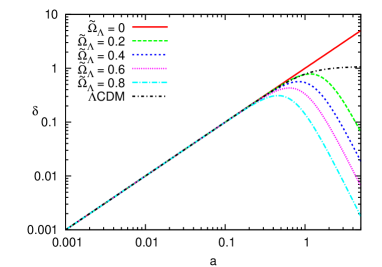
Figure 1: $\delta$ as a function of $a$ for the case $c_{eff}^{2}=0$. As discussed in the text, for LJO models this is equivalent to the case $c_{eff}^{2}=c_{s}^{2}$ because the sound speed is zero. For comparison we also show the flat $\Lambda$CDM case, with $\Omega_{m}=1-\Omega_{\Lambda}=0.3$ and $c_{eff}^{2}=0$.

This case is also interesting because the condition for the Neo-Newtonian perturbed equations to be equivalent to the full general-relativistic treatment for a single fluid is that $c_{eff}^{2}=0$ Reis2003 .

Another interesting choice to the effective sound speed is $c_{eff}^{2}=c_{s}^{2}={\dot{p_{c}}}/{\dot{\rho}}$. In this case, the non-adiabatic pressure, $\delta p_{nad}\approx\delta p_{c}-c_{s}^{2}\delta\rho$ vanishes, and one has only adiabatic perturbations as suggested by CMB observations. However, the sound speed of matter in the presence of particle production reads

$$c_{s}^{2}=\frac{H\Gamma^{\prime}-\Gamma H^{\prime}-\Gamma(3H-\Gamma)}{3H(3H-\Gamma)},$$ (52)

which vanishes identically when the creation rate is given by Eq.(43) since $\dot{p_{c}}\equiv 0$. Therefore, in the LJO framework, this choice for the effective sound speed reduces to the case earlier analyzed ($c_{eff}^{2}=0$). Of course, since $c_{eff}^{2}$ is a new degree of freedom, a possibility is to choose it as a general time dependent variable, say, $c_{eff}^{2}=w$. The treatment involving $c_{eff}^{2}$ as a new degree of freedom is relevant when the unperturbed fluid equations evolve out of thermodynamic equilibrium as in the case of LJO model.

In Figure 1, we display the evolution of the density contrast for LJO model as predicted by the Neo-Newtonian approach. Note that the increasing mode perturbation grows until its maximum value after which it decays in the course of the evolution. In particular, for $\tilde{\Omega}_{\Lambda}=0.2$, we see that the predicted density contrast is indistinguishable from that of $\Lambda$CDM cosmology. However, we stress that such a value is not favored by the background tests which prefer $\tilde{\Omega}_{\Lambda}=0.7$ LJO ; BasLim .

In Figure 2, we display the case $c^{2}_{eff}=w=-\Gamma/3H$. As shown there, the evolution of the density contrast has been obtained for different values of ${\tilde{\Omega}}_{\Lambda}$. Evidently, for $0.2\leq{\tilde{\Omega}}_{\Lambda}\leq 0.4$ the evolution is similar to the $\Lambda$CDM behavior.

As it appears, the simplest possibility to the quantity $c_{eff}^{2}$ is to consider it as a constant free parameter and find out which value is preferred from observations. In this case, $c_{eff}^{2}{}^{\prime}\equiv 0$ and now we have:

$$F(\eta) = \frac{(1-\tilde{\Omega}_{\Lambda})(1+6c_{eff}^{2})+2\tilde{\Omega}_{\Lambda}e^{3\eta}(8+3c_{eff}^{2})}{2(1-\tilde{\Omega}_{\Lambda}+\tilde{\Omega}_{\Lambda}e^{3\eta})}$$ (53)

$$G(\eta) = \frac{9(1-\tilde{\Omega}_{\Lambda})^{2}}{2(1-\tilde{\Omega}_{\Lambda}+\tilde{\Omega}_{\Lambda}e^{3\eta})^{2}}+\frac{15\tilde{\Omega}_{\Lambda}e^{3\eta}(1+c_{eff}^{2})-3(1-\tilde{\Omega}_{\Lambda})(2+c_{eff}^{2})}{1-\tilde{\Omega}_{\Lambda}+\tilde{\Omega}_{\Lambda}e^{3\eta}}+\frac{e^{\eta}k^{2}c_{eff}^{2}}{H_{0}^{2}(1-\tilde{\Omega}_{\Lambda}+\tilde{\Omega}_{\Lambda}e^{3\eta})}$$ (54)

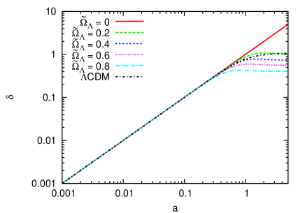
Figure 2: $\delta$ as a function of $a$ for the case $c_{eff}^{2}=w$. Also shown, for comparison, is the flat $\Lambda$CDM case, with $\Omega_{m}=1-\Omega_{\Lambda}=0.3$ and $c_{eff}^{2}=0$. In this case we have considered the limit of large scales ($k=0$).

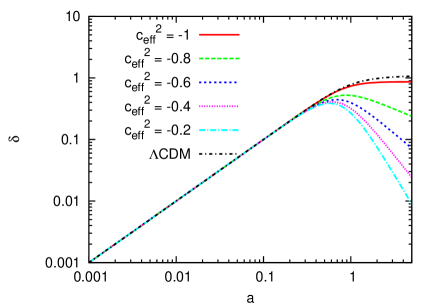
Figure 3: $\delta$ as a function of $a$ for the case in which $c_{eff}^{2}$ is a free parameter. Also shown, for comparison, is the flat $\Lambda$CDM case, with $\Omega_{m}=0.3$ and $c_{eff}^{2}=0$. In this case we have considered the limit of large scales ($k=0$), and $\tilde{\Omega}_{\Lambda}=0.7$.

In Figure 3, we show the evolution of the density contrast when $c^{2}_{eff}$ is taken to be a constant free parameter. The selected values of $c^{2}_{eff}$ are also indicated. Again, we see that there is a range of values for which the CCDM matter fluctuation field mimics the behavior of the concordance $\Lambda$CDM model.

V.1 The growth rate of clustering

We would like to end this section with a discussion on the evolution of the well known indicator of clustering, namely the growth rate peeb93 . This is an efficient parametrization of the linear matter fluctuations $\delta(a)$ which has the following functional form:

$$f(z)=\frac{d{\rm ln}\delta}{d{\rm ln}a}=-(1+z)\frac{d{\rm ln}\delta}{dz}\;.$$ (55)

In Table I, we show the existing growth rate data with the corresponding error bars, the associated redshifts and related references.

Table 1: Data of the growth rate of clustering. The correspondence of the columns is as follows: redshift, observed growth rate and references.

z	$f_{obs}$	Refs.
0.15	$0.49\pm 0.10$	Colles01 ; Guzzo08
0.35	$0.70\pm 0.18$	Teg06
0.55	$0.75\pm 0.18$	Ross07
0.77	$0.91\pm 0.36$	Guzzo08
1.40	$0.90\pm 0.24$	daAng08
2.42	$0.74\pm 0.24$	Viel04
3.00	$1.46\pm 0.29$	McDon05

Let us now attempt to place constraints on the relevant parameters by performing a standard $\chi^{2}$ minimization procedure between the observationally measured growth rate and that predicted by the LJO cosmology. The best fit to the set of independent parameters ($\tilde{\Omega}_{\Lambda},c_{eff}^{2}$) can be estimated by using a $\chi^{2}$ statistics with

$$\chi^{2}(\tilde{\Omega}_{\Lambda},c_{eff}^{2})=\sum_{i=1}^{7}\left[\frac{f_{obs}(z_{i})-f_{\rm model}(z_{i},\tilde{\Omega}_{\Lambda},c_{eff}^{2})}{\sigma_{i}}\right]^{2}\;\;,$$ (56)

where $\sigma_{i}$ is the observed growth rate uncertainty. Note that we sample the free parameters as follows: $\tilde{\Omega}_{\Lambda}\in[0.1,1]$ and $c_{eff}^{2}\in[-1.3,2]$ in steps of 0.001.

In Figure 4 (upper panel), we show the 1$\sigma$, 2$\sigma$ and 3$\sigma$ confidence levels in the $(\tilde{\Omega}_{\Lambda},c_{eff}^{2})$ plane. It is evident that $c_{eff}^{2}$ is degenerate with respect to $\tilde{\Omega}_{\Lambda}$ and that all the values on the interval $-1.3\leq c_{eff}^{2}\leq 2$ are acceptable within the $1\sigma$ uncertainty. As one may check, the $c_{eff}^{2}$ parameter as a function of $\tilde{\Omega}_{\Lambda}$ is well fitted by a power law having the form:

$$c_{eff}^{2}=0.333(\pm 0.011)\tilde{\Omega}_{\Lambda}^{-0.989(\pm 0.021)}-1.5\;.$$

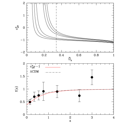
Figure 4: Upper Panel: Likelihood contours in the $(\tilde{\Omega}_{\Lambda},c_{eff}^{2})$ plane. The contours are plotted where $-2{\rm ln}({\cal L/L_{\rm max}})$ is equal to 2.32, 6.16 and 11.83, corresponding to $1\sigma$, $2\sigma$ and $3\sigma$ confidence level. The perpendicular dashed line separates the regions in which the flat LJO model can accommodate an accelerated expansion ($\tilde{\Omega}_{\Lambda}>1/3$), equivalent to the standard $\Lambda$CDM cosmology. Bottom Panel: Comparison of the observed (solid circles see Table I) and theoretical evolution of the growth rate of clustering $f(z)$. Note that we have imposed $\tilde{\Omega}_{\Lambda}=0.7$ as suggested by the background tests LJO ; BasLim . The lines correspond to the LJO (solid curve with $c_{eff}^{2}=-1$) and the $\Lambda$CDM (dot-dashed curve with $\Omega_{\Lambda}\equiv\tilde{\Omega}_{\Lambda}$ and $c_{eff}^{2}\equiv 0$) models.

It is also evident that the likelihood analysis puts some constraints on the value of $c_{eff}^{2}$ once including the necessary condition for an inflection point, that is, a transition from a decelerating to an accelerating regime in our past. Thus, for $\tilde{\Omega}_{\Lambda}>1/3$, (see dashed line in the upper panel of figure 4) we find that $c_{eff}^{2}$ lies in the interval $-1.24\leq c_{eff}^{2}\leq-0.72$. In this framework, if we marginalize over $\tilde{\Omega}_{\Lambda}=0.7$, then the likelihood analysis provides a best fit value of $c_{eff}^{2}\simeq-1$ with $\chi^{2}\simeq 4.03$ (${\rm dof}=6$). The latter result remains unaltered within a physical range of $0.65\leq\tilde{\Omega}_{\Lambda}\leq 0.74$. Of course, for comparison we perform the same analysis also for the $\Lambda$CDM model ($\Omega_{\Lambda}=0.7$) and we find $\chi^{2}\simeq 4.88$ (${\rm dof}=7$).

In the bottom panel of Figure 4, we present the LJO growth rate of clustering (solid line). We find that for $z\leq 1$ the LJO growth rate is somewhat less with respect to that of the usual $\Lambda$ cosmology (dot-dashed line) and such a difference increases for extremely low redshifts. However, at relatively large redshifts ($z>1$) the growth rate of the LJO model is indistinguishable from that of the $\Lambda$CDM model. This should be expected because the flat LJO model reduces to the Einstein - de Sitter cosmology at intermediate and high $z$’s (negligible particle production). Note that the measured $f_{obs}(z)$ are presented in the bottom panel of Fig. 4 by the filled symbols.

We further explore our statistical results by using a Bayesian statistics (see for example essence ), in which the corresponding estimator is defined as: $BIC=\chi^{2}+k_{n}{\rm ln}N$ [where $k_{n}$ is the number of free parameters and $N(\equiv 7)$ is the number of data points used in the fit]. The next step is to estimate the relative deviation between the two models $\Delta BIC=BIC_{LJO}-BIC_{\Lambda}$. In general a difference in $BIC$ of $\Delta BIC>6$, is considered evidence against that model which occurs the larger $BIC$. In our case, we find $\Delta BIC\simeq 1.01$ which implies that the LJO model with $(\tilde{\Omega}_{\Lambda},c_{eff}^{2})=(0.70,-1)$ fits very well the growth rate data. The latter result holds also for $0.65\leq\tilde{\Omega}_{\Lambda}\leq 0.74$.

Secondly, we compare the growth rate of clustering between data and models via a Kolmogorov-Smirnov (KS) statistical test respectively by computing the corresponding consistency between models and data (${\cal P}_{KS}$). Although both cosmological models fit well the data it seems that the LJO model provides a slightly better fit (${\cal P}_{KS}\simeq 0.997$) with respect to that of the usual $\Lambda$ cosmology (${\cal P}_{KS}\simeq 0.883$). Note that the KS test between the two cosmological models gives ${\cal P}_{KS}\simeq 1$.

Based on the above statistical tests it becomes evident that in the LJO model ($0.65\leq\tilde{\Omega}_{\Lambda}\leq 0.74$, $c_{eff}^{2}=-1$), the corresponding Hubble flow as well as the matter fluctuation field resembles that of the traditional $\Lambda$CDM cosmology without the need of the required, in the classical cosmological models, dark energy.

At this point one may ask about the possibility of future detection or at least what is a clear cosmic signature of this gravitationally induced creation process of cold dark matter particles. As it is widely known, some very massive dark matter particle candidates like the wimpzillas ($M_{W}\sim 10^{13}$ GeV) can be copiously produced only at the very early stages of the Universe, mainly at the end of inflation KST ; PDM , and, as such, this kind of candidate does not fit in our phenomenological treatment for continuous matter creation. In principle, a more realistic scenario is provided by the semi-classical approach proposed by Parker and collaborators Parker , where massive particles (associated to a real scalar field) can be continuously created during the expansion of the Universe. On the other hand, since the current dark matter detection experiments rely on the physical properties of the dark matter (mass, cross section, etc), we are unable to identify (based only on our phenomenological approach) which is the specific candidate for the continuous cold dark matter production discussed here. However, by assuming that the created mass are of the form of neutralinos ($M_{N}\sim 100GeV$), one may show that its present creation rate, $\Gamma_{neu}\sim 10^{-11}$ cm^-3yr^-1, has not changed appreciably in the last few billion years when the Universe entered its accelerating phase LJO .

VI Conclusions

The problem related to the nature of non-baryonic component filling the observed Universe is usually referred to as the non-baryonic dark matter problem. In the last three decades, many possible candidates from particle physics have been proposed to describe such a dark matter component PDM . In the framework of general relativity, it is also interesting to know whether the dark sector (dark matter + dark energy) could be properly reduced only to the dark matter component with the conventional $\Lambda$CDM emerging as an effective description LJO ; BasLim . Naturally, unlike the decelerating dust-filled Einstein-de Sitter Universe, an extra mechanism must be responsible for the present observed accelerating stage.

In this context, we have performed a Neo-Newtonian description of relativistic CCDM models, that is, models endowed with gravitationally induced production of cold dark matter particles. The complete equivalence of the Neo-Newtonian cosmological approach with the general relativistic background equations regardless of the specific form adopted to the particle production rate, $\Gamma$, has been established. In the same vein, the general perturbed equations has also been derived in this framework. Due to the form of the negative creation pressure ($p_{c}=-\Gamma\rho/3H$) we have determined the general differential equation to the contrast density by assuming a full equivalence to a fluid model with an EoS parameter $w=-{\Gamma}/{3H}$. The resulting equations of section IV are also valid for arbitrary forms of $\Gamma$.

In section V, we have focused our attention to a specific CCDM cosmology, namely, the LJO model LJO . The interest for this special class of CCDM cosmology comes from the fact that its expanding history is equivalent to the standard $\Lambda$CDM model.

Three different perturbed scenarios depending on the choice of the $c_{eff}^{2}$ were analyzed. In the first one $c_{eff}^{2}=c_{s}^{2}=0$ and the linear perturbation is equivalent to that predicted by $\Lambda$CDM only up to redshifts of the order of one. It was found that the increasing mode decays rapidly after $z\sim 1$ with the redshift marking the beginning of attenuation depending on the $\tilde{\Omega}_{\Lambda}$ parameter (see Fig. 1). We also show that the nonadiabatic case with $c_{eff}^{2}=\omega$ is equivalent to a perturbed $\Lambda$CDM, however, only for $0.2\leq{\tilde{\Omega}}_{\Lambda}\leq 0.4$ (see Fig. 2). Finally, when $c_{eff}^{2}$ was treated as a free constant parameter, the perturbed evolution is like $\Lambda$CDM for $\tilde{\Omega}_{\Lambda}=0.7$ (see Fig. 3) which is exactly the same value preferred by the expanding cosmic history LJO . For all these models, it should be interesting to obtain the predicted matter power spectrum in the context of the relativistic formulation. This work is in progress and will be published elsewhere.

For completeness, we also performed a detailed statistical analysis based on the observed growth rate of clustering in order to constrain the free parameters ($\tilde{\Omega}_{\Lambda},c_{eff}^{2}$). Interestingly, when combined with the background tests LJO ; BasLim , the best fit values are $\tilde{\Omega}_{\Lambda}=0.7$ and $c_{eff}^{2}=-1$ (compare Figs. 3 and 4). In this case, the LJO pattern predicts an overall dynamics (Hubble flow and matter fluctuation field) which is for all practical purposes indistinguishable from the traditional $\Lambda$ cosmology. Naturally, such a solution based on a reduction of the dark sector, provides not only a possible reinterpretation of the $\Lambda$CDM cosmology but also offers a viable alternative cosmic scenario to the late time accelerating Universe without the need of an exotic dark energy. Indeed one of the main advantages of such CCDM cosmology is the fact that it contains the same number of free parameters as the concordance $\Lambda$CDM model, and, therefore, it does not require the introduction of any extra fields in its dynamics.

References

- (1) A. Riess et al., Astron. J. 116, 1009 (1998); S. Perlmutter et al., Astrophys. J. 517, 565 (1999).
- (2) Kowalski et al., Astrophys. J. 686 749 (2008).
- (3) M. Hicken et al., Astrophys. J. 700, 1097 (2009).
- (4) R. Amanullah et al., arXiv:1004.1711 (2010).
- (5) S. Weinberg, Rev. Mod. Phys. 61, 1 (1989).
- (6) P. J. Peebles and B. Ratra, Rev. Mod. Phys. 75, 559 (2003); T. Padmanabhan, Phys. Rep. 380, 235 (2003); J. A. S. Lima, Brazilian J. of Physics, 34 194 (2004); J. A. Frieman, M. S. Turner and D. Huterer, Ann. Rev. Astron. & Astrophys. 46, 385 (2008).
- (7) I. Zlatev, L. Wang, and P. J. Steinhardt, Phys. Rev. Lett. 82, 896 (1999); L. P. Chimento, A. S. Jakubi, D. Pavon, and W. Zimdahl, Phys. Rev. D 67, 083513 (2003); S. Nojiri and S. D. Odintsov, Phys. Lett. B 637, 139 (2006); M. Quartin, M. O. Calvão, S. E. Joras, R. R. R. Reis, and I. Waga, JCAP 05, 007 (2008).
- (8) S. del Campo, R. Herrera, and D. Pavon, Phys. Rev. D78, 021302 (2008); E. Abdalla, L. R. Abramo, and J. C. C. de Souza, Phys. Rev. D 82, 023508 (2010); S. Z. W. Lip, Phys. Rev. D 83, 023528 (2011).
- (9) A. Blanchard, M. Douspis, M. Rowan-Robinson and S. Sarkar, Astron. and Astrophys. 412, 35 (2003).
- (10) Many different aspects of dark matter candidates can be seen in “Particle Dark Matter: Observations, Models and Searches”, edited by G. Bertone, Cambridge University Press (2010).
- (11) I. Prigogine et al., Thermodynamics and Cosmology, Gen. Rel. Grav., 21, 767 (1989).
- (12) J. A. S. Lima, M. O. Calvão, I. Waga, “Cosmology, Thermodynamics and Matter Creation”, Frontier Physics, Essays in Honor of Jayme Tiomno, World Scientific, Singapore (1990), [arXiv:0708.3397]; M. O. Calvão, J. A. S. Lima and I. Waga, Phys. Lett. A162, 223 (1992). See also, J. A. S. Lima and A. S. M. Germano, Phys. Lett. A 170, 373 (1992).
- (13) J. A. S. Lima, A. S. M. Germano and L. R. W. Abramo, Phys. Rev. D53, 4287 (1996), (arXiv:gr-qc/9511006); L. R. W. Abramo and J. A. S. Lima, Class. Quantum Grav. 13, 2953 (1996), arXiv:gr-qc/9606064; J. A. S. Lima and J. S. Alcaniz, Astron. Astrophys. 348 1 (1999), arXiv:astro-ph/9902337; W. Zimdhal, D. J. Schwarz, A. B. Balakin, and D. Pavo n, Phys. Rev. D 64, 063501 (2001); M. P. Freaza, R. S. de Souza, and I. Waga, Phys. Rev. D 66, 103502 (2002); J. A. S. Lima, F. E. Silva and R. C. Santos, Class. Quant. Grav. 25, 205006 (2008), (arXiv:0807.3379); S. Basilakos and M. Plionis, Astron. & Astrophys. 507, 47 (2009).
- (14) G. Steigman, R. C. Santos and J. A. S. Lima, JCAP 06, 033 (2009), arXiv:0812.3912 [astro-ph].
- (15) J. A. S. Lima, J. F. Jesus and F. A. Oliveira, JCAP 11, 027 (2010), arXiv:0911.5727 [astro-ph.CO].
- (16) S. Basilakos and J. A. S. Lima, Phys. Rev. D.82, 023504 (2010), arXiv:1003.5754 [astro-ph.CO].
- (17) S. Basilakos M. Plionis and J. A. S. Lima, Phys. Rev. D82, 083517 (2010), arXiv:1006.3418 [astro-ph.CO].
- (18) J. A. S. Lima, V. Zanchin and R. Brandenberger, Mon. Not. R. Astron. Soc. 291, L1 (1997).
- (19) McCrea W. H., Proc. Roy. Soc. A, 206, 562 (1951).
- (20) Harrison E. R., Annals of Phys., 35, 437 (1965).
- (21) R. R. R. Reis, Phys. Rev. D 67, 087301 (2003). [Erratum-ibid. D 68, 089901 (2003)].
- (22) A. Nayeri and T. Padmanabhan, arXiv:gr-qc/9807039v2.
- (23) L. R. Abramo, R. C. Batista, L. Liberato and R. Rosenfeld, JCAP 11, 012 (2007).
- (24) A. de Roany and J. A. d. Pacheco, Gen. Rel. Grav. (2011). In press, DOI:10.1007/ s10714-010-1069-2, arXiv:1007.4546 [gr-qc].
- (25) J. A. S. Lima, J. F. Jesus and F. A. Oliveira, Gen. Rel. Grav. (2011). In press, DOI 10.1007/s10714-011-1161-2, arXiv:1012.5069 [astro-ph.CO].
- (26) P. J. E. Peebles, The Large Scale Structure of the Universe, Princeton University Press, Princeton (1980).
- (27) P. J. E. Peebles, Principles of Physical Cosmology, Princeton University Press, Princeton (1993).
- (28) J. Garriga and V. F. Mukhanov, Phys. Lett. B 458, 219 (1999). [arXiv:hep-th/9904176].
- (29) M. Colless et al., Mon. Not. Roy. Astron. Soc., 328, 1039 (2001).
- (30) L. Guzzo et al., Nature, 451, 541 (2008).
- (31) M. Tegmark et al., Phys. Rev. D., 74, 123507 (2006).
- (32) N. P. Ross et al., Mon. Not. Roy. Astron. Soc., 381, 573 (2007).
- (33) J. da Angela et al., Mon. Not. Roy. Astron. Soc., 383, 565 (2008)
- (34) M. de Viel, M. G. Haehnelt and V. Springel, Mon. Not. Roy. Astron. Soc., 354, 684, (2004)
- (35) P. McDonald, et al., Astrophys. J., 635, 761 (2005).
- (36) T. M. Davis et al., Astrophys. J., 666, 716 (2007).
- (37) E. W. Kolb, A. A. Starobinsky and I. I. Tkachev, JCAP 07 005 (2007).
- (38) L. Parker, Phys. Rev. 183 1057, (1969); L. Parker and A. Raval, Phys. Rev. Lett. 86, 749 (2001); L. Parker and D. A. T. Vanzella, Phys. Rev. D 69, 104009 (2004).