Supercurrent and Andreev bound state dynamics in superconducting quantum point contacts under microwave irradiation

Abstract

We present here an extensive theoretical analysis of the supercurrent of a superconducting point contact of arbitrary transparency in the presence of a microwave field. Our study is mainly based on two different approaches: a two-level model that describes the dynamics of the Andreev bound states in these systems and a fully microscopic method based on the Keldysh-Green function technique. This combination provides both a deep insight into the physics of irradiated Josephson junctions and quantitative predictions for arbitrary range of parameters. The main predictions of our analysis are: (i) for weak fields and low temperatures, the microwaves can induce transitions between the Andreev states leading to a large suppression of the supercurrent at certain values of the phase, (ii) at strong fields, the current-phase relation is strongly distorted and the corresponding critical current does not follow a simple Bessel-function-like behavior, and (iii) at finite temperature, the microwave field can enhance the critical current by means of transitions connecting the continuum of states outside the gap region and the Andreev states inside the gap. Our study is of relevance for a large variety of superconducting weak links as well as for the proposals of using the Andreev bound states of a point contact for quantum computing applications.

I Introduction

In 1962 Josephson predicted that a dissipationless current (supercurrent) could flow in a junction between two superconductors (S) weakly coupled by an insulating barrier,Josephson1962 which was confirmed experimentally shortly afterwards by Anderson and Rowell.Anderson1963 Soon after this confirmation, it became clear that this phenomenon, referred to as the dc Josephson effect, could take place in a variety of superconducting weak links such as Dayem bridges, SNS junctions, where N corresponds to a normal metal bridge, or large point contacts.Likharev1979 ; Barone1982 The only difference between these systems lies on the exact current phase relation (CPR), which depends on the characteristics of the constriction linking the superconducting leads.Golubov2004

In recent years, the dc Josephson effect has been investigated in novel superconducting junctions with weak links based on atomic contacts,Koops1996 ; Goffman2000 ; Rocca2007 carbon nanotubes,Kasumov1999 ; Jarillo-Herrero2006 ; Jorgensen2006 fullerenes,Kasumov2005 semiconductor nanowires,Doh2005 ; Xiang2006 or graphene.Heersche2007 ; Du2008 ; Jeong2011 Some of these nanostructures fall into the category of a superconducting quantum point contact (SQPC), where the constriction has a length much smaller than the superconducting coherence length. In this limit, and in the absence of strong interactions in the constriction, the dc Josephson effect can be described in a unified manner using two basic concepts of mesoscopic physics, namely the concepts of conduction channels and Andreev bound states. In the normal state, the coherent transport through a mesoscopic system can be described in terms of the independent contributions of the eigenfunctions of the transmission matrix from the structure, known as conduction channels, and these contributions are determined by the corresponding transmission coefficients $\{\tau_{i}\}$. In the superconducting state, the electrons (holes) transmitted in a conduction channel are Andreev reflected at the electrodes as holes (electrons) in the same channel. This process is successively repeated in both electrodes leading to the formation of a pair of bound states in the gap region. These are known as the Andreev bound states (ABSs). In the case of a single-channel SQPC with transmission $\tau$, the energies of the ABSs are given byFurusaki1991 ; Beenakker1991

$$E^{\pm}_{\rm A}(\varphi,\tau)=\pm E_{\rm A}(\varphi,\tau)=\pm\Delta\sqrt{1-\tau\sin^{2}(\varphi/2)},$$ (1)

where $\Delta$ is the superconducting gap and $\varphi$ is the phase difference between the order parameters on both sides of the junction. In equilibrium, these two states carry opposite supercurrents $I^{\pm}_{\rm A}(\varphi)=(2e/\hbar)\partial E^{\pm}_{\rm A}/\partial\varphi$, which are weighted by the occupation of the ABSs (determined by the Fermi function). In the case of a multichannel SQPC, the supercurrent is simply given by the sum of the contributions from the individual channels.Beenakker1991

This unified microscopic picture of the dc Josephson effect has been confirmed experimentally in the context of atomic contacts by Della Rocca and coworkers.Rocca2007 In particular, these authors measured the CPR of an atomic contact placed along with a tunnel junction in a small superconducting loop and found an excellent agreement with the theory using the independently determined transmission coefficients. At this stage, one may wonder whether it is possible to control the occupation of ABSs of a SQPC with an external field, and in turn to control the supercurrent. This is the main issue explored in this work and for this purpose, we present here an extensive theoretical analysis of the supercurrent and the dynamics of the ABSs of a SQPC under microwave irradiation. This is a basic problem in mesoscopic superconductivity, which is also relevant for the field of quantum computing since the ABSs of a SQPC have been proposed to be used as the two states of a qubit.Desposito2001 ; Zazunov2003 ; Zazunov2005 In this proposal, a microwave field can be used for the spectroscopy of the two-level system or to probe its quantum state by current measurements.

The microwave-assisted supercurrent in SQPCs is often discussed in the framework of the adiabatic approximation (see Section II), where one assumes that the ABSs follow adiabatically the microwave field. This approximation does not take into account the possible transitions between the ABSs and therefore, if fails to describe the current at high frequencies or for highly transmissive contacts, where the energy difference between the states can be rather small. The first microscopic analysis of this problem for a SQPC of an arbitrary transparency was reported by Shumeiko and coworkers.Shumeiko1993 These authors studied the limit of weak fields and predicted the possibility to have a large suppression of the current due to resonant transitions between the ABSs. Later, other aspects of this problem, including the dynamics of the ABSs, have been addressed focusing on the linear response regime.Gorelik1995 ; Gorelik1998 ; Lundin2000 A complete solution of this problem, valid for an arbitrary range of parameters, has only been reported very recently.Bergeret2010 In this latter work, we developed a theory of the supercurrent through a microwave-irradiated SQPC in the framework of the Keldysh-Green function technique. This theory allowed us to put forward new predictions such as the evolution of the CPR with the radiation power and the possibility to enhance the critical current at finite temperatures by irradiating the junction. Here, we describe in detail this theory (see Section IV) and, in particular, we present new analytical results that elucidate the origin of the microwave-enhanced supercurrents.

In the process of understanding the results of the exact theory, we are confronted with the question of to what extent the physics of microwave-irradiated SQPCs can be understood in terms of just the dynamics of the ABSs, i.e., in terms of a natural extension of the argument described in the previous paragraphs for the case of a junction in equilibrium. In order to answer this question, we make use of the two-level Hamiltonians of a SQPC existing in the literatureIvanov1999 ; Zazunov2003 and we compare the results with the exact theory. This comparison serves in turn to establish the range of validity of these two-level models. It is worth stressing that within these models the computation of the dc properties such as the supercurrent or the average occupation of the ABSs for arbitrary radiation is a highly non-trivial task. In order to carry it out, we have developed a new powerful method which allows us to compute any dc quantity in an arbitrary two-level system driven out of equilibrium by a periodic perturbation. This method is described in Section III and it constitutes one of the main results of this work. With the help of this method, we show that with the Hamiltonian of Ref. Zazunov2003, one can nicely reproduce the exact results at low temperatures and low radiation powers. Moreover, this analysis allows us to obtain analytical results for the supercurrent dips produced by microwave-induced transitions between the ABSs.

The rest of the paper is organized as follows. In the next section we briefly review the equilibrium properties of a SQPC as well as the basic results of the adiabatic approximation. In Section III we study the dynamics of the ABSs under a microwave field within the two-level Hamiltonian of Ref. Zazunov2003, . In particular, we describe a novel method that allows us to obtain the CPR for any power and frequency of the external field, and we also derive analytical expressions for the supercurrent beyond the rotating wave approximation. In Section IV we discuss the Keldysh-Green function technique, which describes the supercurrent for an arbitrary range of parameters, including also the contribution of the continuum of states outside the gap region. We present a detailed comparison of the results of this technique at zero temperature with those obtained with the two-level model. Moreover, we analyze in detail the phenomenon of microwave-enhanced supercurrent at finite temperatures, for which we present analytical results. Finally, Section V is devoted to some additional discussions and to summarizing the main results of this work.

II System and adiabatic approximation

We consider a SQPC consisting of two identical superconducting electrodes with an energy gap $\Delta$, linked by a single conduction channel of transmission $\tau$. Our main goal is to compute the supercurrent through this system when it is subjected to a monochromatic microwave field of frequency $\omega$. We assume that the external radiation generates a time-dependent voltage $V(t)=V_{0}\sin\omega t$,Barone1982 where the amplitude $V_{0}$ depends on the power of the external radiation source, and eventually also on the polarization of the radiation. According to the Josephson relation, this voltage induces a time-dependent superconducting phase difference given by

$$\phi(t)=\varphi+2\alpha\cos\omega t,$$ (2)

where $\varphi$ is the dc part of the phase and $\alpha=eV_{0}/\hbar\omega$ is a parameter that measures the strength of the coupling to the electromagnetic field and it is used here as a parameter to be determined by comparing with the experiments.

As explained in the introduction, in the absence of microwaves the supercurrent can be expressed as a sum of the contributions of the two ABSs as $I_{\rm eq}(\varphi)=I^{-}_{\rm A}n_{\rm F}(E^{-}_{\rm A})+I^{+}_{\rm A}n_{\rm F}(E^{+}_{\rm A})$, $n_{\rm F}(E)$ being the Fermi distribution function, which yieldsHaberkorn1978

$$I_{\rm eq}(\varphi)=\frac{e\Delta^{2}}{2\hbar}\frac{\tau\sin\varphi}{E_{\rm A}(\varphi)}\tanh\left(\frac{E_{\rm A}(\varphi)}{2k_{\rm B}T}\right),$$ (3)

where $E_{\rm A}$ is defined in Eq. (1) and $T$ is the temperature. In the tunnel regime ($\tau\ll 1$), this expression reduces to the sinusoidal CPR given by the Ambegaokar-Baratoff formula:Ambegaokar1963 $I_{\rm eq}(\varphi)=I_{\rm C}\sin\varphi$, with $I_{\rm C}=(e\Delta\tau/2\hbar)\tanh(\Delta/2k_{\rm B}T)$. At perfect transparency ($\tau=1$), this expression reproduces the Kulik-Omelyanchuk formula:Kulik1977 $I_{\rm eq}(\varphi)=I_{0}\sin(\varphi/2)\tanh(\Delta\cos(\varphi/2)/2k_{\rm B}T)$. Here, $I_{0}=e\Delta/\hbar$ is the zero-temperature critical current for $\tau=1$ and we frequently use it below to normalize the supercurrent in the different graphs. According to Eq. (3), at zero temperature only the lower ABS contributes to the supercurrent $I_{\rm eq}=I^{+}_{\rm A}$, while at a finite temperature the negative contribution from the upper ABS leads to a decrease of the total supercurrent.

The simplest approach to compute the supercurrent in the presence of the microwave field is the so-called adiabatic approximation.Barone1982 In this approximation one assumes that the ABSs follow adiabatically the ac drive and there are no direct transitions between them. Thus, the CPR in this approximation is obtained by replacing the stationary phase $\varphi$ in Eq. (3) by the time-dependent phase $\phi(t)$ of Eq. (2), which leads to the following result

$$I_{\rm ad}(\varphi,\alpha)=\sum_{n=1}^{\infty}I_{n}J_{0}(2n\alpha)\sin(n\varphi),$$ (4)

where $I_{n}=(1/\pi)\int_{0}^{2\pi}d\varphi\;I_{\rm eq}(\varphi)\sin(n\varphi)$ are the harmonics of the equilibrium CPR of Eq. (3) and $J_{0}$ is the zero-order Bessel function of the first kind. Notice that the current in this approximation does not depend explicitly on the radiation frequency. We illustrate the results of this approximation in Fig. 1 for the zero-temperature case. In particular, in the two upper panels we show the CPR (obtained from Eq. (4)) for two different transmissions and several values of the $\alpha$ parameter (related to the microwave power). Panel (a) corresponds to the tunnel limit ($\tau=0.2$) where the CPR is sinusoidal irrespective of the radiation power, while in panel (b) we show the results for a high transmission of $\tau=0.95$. In this latter case, the critical current is reached at different values of the phase depending on the value of $\alpha$. Notice that no matter the value of the phase $\varphi$, the magnitude of the supercurrent is always suppressed by the microwaves as compared with the zero-field result ($\alpha=0$), which is true at any temperature. With respect to the behavior of the critical current $I_{C}(\alpha)$, as one can see in Fig. 1(c), it decays in a non-monotonic manner, as governed by the Bessel function $J_{0}$.

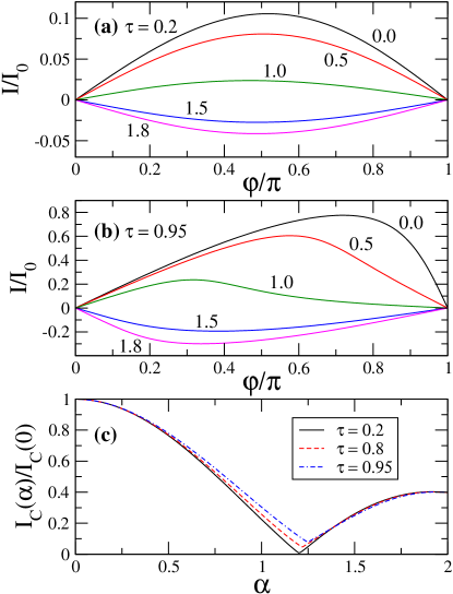
Figure 1: (Color online) Panels (a) and (b): The current-phase relation in the adiabatic approximation for $\tau=0.2$ (a) and $\tau=0.95$ (b). The different curves correspond to different values of $\alpha$ as indicated in the graphs. The current is given in units of $I_{0}=e\Delta/\hbar$, where $\Delta$ is the value of the superconducting gap at $T=0$. (c) The zero-temperature critical current as a function of $\alpha$ for three different values of the transmission $\tau$. Notice that critical current is normalized by its value in the absence of microwaves.

III The two-level model

It is instructive to start our analysis towards a microscopic theory by restricting ourselves to the study of the contribution of ABSs, ignoring for the moment the continuum part of the spectrum. This can be done with the help of the two-level models that have been derived in Refs. Ivanov1999, and Zazunov2003, to describe the dynamics of a SQPC under external ac fields. The models of these two references coincide at equilibrium, but they differ slightly when the phase depends on time. In particular, the model of Ref. Zazunov2003, ensures charge neutrality, while the model of Ref. Ivanov1999, does not. For this reason, we base our discussion here on the model put forward by Zazunov and coworkers.Zazunov2003 In this model, the SQPC is described by the $2\times 2$ Hamiltonian

$$\hat{H}_{\rm B}(t)=\Delta e^{-i\hat{\sigma}_{x}r\phi/2}\left(\cos\frac{\phi}{2}\hat{\sigma}_{z}+r\sin\frac{\phi}{2}\hat{\sigma}_{y}\right)\;,$$ (5)

where $r=\sqrt{1-\tau}$ and $\phi(t)$ is the time-dependent phase given by Eq. (2). This Hamiltonian is written in the ballistic basis of right- and left moving electrons, which are eigenvectors of the current operator in the perfectly transmitting case ($\tau=1$). For our subsequent analysis it is more convenient to work in the instantaneous Andreev basis $\{\lvert+\rangle_{\phi(t)}$, $\lvert-\rangle_{\phi(t)}\}$, whose basis vectors are time-dependent. This is the basis where the Hamiltonian of Eq. (5) becomes diagonal in equilibrium. The Andreev basis is obtained from the ballistic basis by means of a transformation $\hat{H}_{A}(t)=\hat{R}^{\dagger}(t)\hat{H}_{B}(t)\hat{R}(t)$ generated by the unitary matrix

$$\hat{R}(t)=e^{-i\hat{\sigma}_{x}r\frac{\phi}{4}}e^{-i\frac{\pi}{4}\hat{\sigma}_{z}}e^{-i\theta(\phi)\hat{\sigma}_{y}},$$ (6)

where $\theta(\phi)=(1/2)\arctan[r\tan(\phi/2)]$. With this transformation the Schrödinger equation for a state vector $\Psi(t)=(\alpha(t),\beta(t))^{T}$ becomes

$$i\partial_{t}\Psi(t)=\hat{H}_{\rm A}(t)\Psi(t)\;,$$ (7)

where

$$\hat{H}_{\rm A}(t)=E_{\rm A}(\phi(t))\hat{\sigma}_{z}-\frac{r\tau\Delta^{2}\sin^{2}(\phi(t)/2)}{4[E_{\rm A}(\phi(t))]^{2}}\dot{\phi}(t)\hat{\sigma}_{y},$$ (8)

and $\dot{\phi}(t)=\partial\phi(t)/\partial t$. Moreover, in the previous two equations, and in the rest of this section, we set $\hbar=1$.

The corresponding current operator can be written as

$$\hat{I}_{\rm A}(t)=2eE^{\prime}_{\rm A}(\phi(t))\hat{\sigma}_{z}+\frac{er\tau\Delta^{2}\sin^{2}(\phi(t)/2)}{E_{\rm A}(\phi(t))}\hat{\sigma}_{x},$$ (9)

where the prime in $E^{\prime}_{\rm A}$ means derivative with respect to the argument (the time-dependent phase in this case). To obtain the expectation value of the current at different times, Eq. (7) needs to be solved. Despite the apparent simplicity, this task has nontrivial aspects: straightforward numerical approaches run into problems, as both very fast ($t^{-1}\sim{}\omega$) and very slow ($t^{-1}\sim{}E_{\rm A}-n\omega$) time scales can be simultaneously present. No closed-form analytical solution can be obtained either,Grifoni1998 and the significantly nonlinear coupling to the drive makes it more difficult to derive approximations via standard routes.Bloch1940 ; Autler1955

Focusing our analysis on time-averaged quantities, we can obtain accurate analytical and numerical results via a systematic Floquet-type approach. We are interested in two physical quantities: the dc current

$$\bar{I}=\lim_{t\to\infty}\frac{1}{t}\int_{0}^{t}dt^{\prime}\Psi^{\dagger}(t^{\prime})\hat{I}(t^{\prime})\Psi(t^{\prime})\,,$$ (10)

and the time-averaged populations of the Andreev levels

$$\bar{p}_{\pm}=\lim_{t\to\infty}\frac{1}{t}\int_{0}^{t}dt^{\prime}\Psi^{\dagger}(t^{\prime})\frac{\hat{1}\pm\hat{\sigma}_{z}}{2}\Psi(t^{\prime})\;.$$ (11)

Below, we show how to obtain $\bar{I}$, although the method described can as well be used to compute any other time-averaged quantity, including $\bar{p}_{\pm}$.

We first introduce a modified Hamiltonian

$$\hat{H}_{\rm A}(t,\chi)=\hat{H}_{\rm A}(t)+\chi\hat{I}_{\rm A}(t)\;,$$ (12)

where $\chi$ is a parameter conjugate to the observable, and it is set to zero at the end of the calculation. The solution of the Schrödinger equation $\Psi(t,\chi)$ can be formally written by introducing the time evolution operator $\hat{U}(t,0;\chi)$

$$\Psi(t,\chi)={\cal T}e^{-i\int_{0}^{t}dt^{\prime}\hat{H}_{A}(t^{\prime},\chi)}\Psi_{0}\equiv\hat{U}(t,0;\chi)\Psi_{0}\,,$$ (13)

where ${\cal T}$ indicates time ordering and $\Psi_{0}$ is the state vector at $t=0$. We define now the generating function:

$$S(t,\chi)=\Psi_{0}^{\dagger}U(0,t;\chi=0)U(t,0;\chi)\Psi_{0}\,.$$ (14)

One can easily check that the dc current defined in Eq. (10) can be written as

$$\bar{I}=\lim_{t\to\infty}\frac{i}{t}\partial_{\chi}S(t,\chi)|_{\chi=0}\;.$$ (15)

Thus, we only need to compute the function $S$, or, equivalently, the evolution operator $\hat{U}(t,0;\chi)\equiv\hat{U}(t;\chi)$.

Since our Hamiltonian is periodic in time with a period $T=2\pi/\omega$, i.e., $H_{\rm A}(t,\chi)=H_{\rm A}(t+T;\chi)$, we can define two periodic (Floquet) states ${\rm v}_{\pm}$ via the eigenvalue problem

$$\hat{U}(T;\chi){\rm v}_{\pm}(\chi)=e^{\pm iE(\chi)T}{\rm v}_{\pm}(\chi)\,.$$ (16)

The symmetry of the two eigenvalues follows here from the fact that $\hat{H}_{\rm A}(t,\chi)$ and ${\rm log}[U(T;\chi)]$ are traceless, and $U(T;\chi)$ is unitary. Moreover, from the periodicity of the Hamiltonian it follows that

$$\hat{U}(nT;\chi)=\hat{U}(T;\chi)^{n}=\hat{V}(\chi)e^{iE(\chi)nT\hat{\sigma}_{z}}\hat{V}^{-1}(\chi)\;,$$ (17)

where the eigenvectors ${\rm v}_{\pm}$ form the columns of the unitary matrix $\hat{V}$. Replacing in Eqs. (14) and (15) $t$ by $nT$ and taking the limit $n\rightarrow\infty$ we now find the derivative with respect to $\chi$:

$$\frac{1}{nT}\partial_{\chi}\hat{U}(nT;\chi)\stackrel{{\scriptstyle n\rightarrow\infty}}{{\longrightarrow}}i\hat{V}^{-1}(\chi)\hat{\sigma}_{z}e^{iE(\chi)nT\hat{\sigma}_{z}}\hat{V}(\chi)\frac{\partial E(\chi)}{\partial\chi}\,.$$ (18)

Thus, the dc current is given by

$$\bar{I}=-\Psi_{0}^{\dagger}\left({\rm v}_{+}{\rm v}_{+}^{\dagger}-{\rm v}_{-}{\rm v}_{-}^{\dagger}\right)\Psi_{0}\left.\frac{\partial E(\chi)}{\partial\chi}\right|_{\chi=0}\;.$$ (19)

This exact expression for the dc current is very useful for numerics. It is easy to compute and it handles the fast and slow time scales of the problem separately. In order to obtain the dc current, one needs first to integrate the Schrödinger equation with the Hamiltonian of Eq. (12) over one period to find the $2\times 2$ matrix $\hat{U}(T;\chi)$, then one computes its eigenvalues $\pm{}E$ and eigenvectors ${\rm v}_{\pm}$, and finally the derivative $\partial_{\chi}{}E(\chi)$ is computed via numerical differentiation.

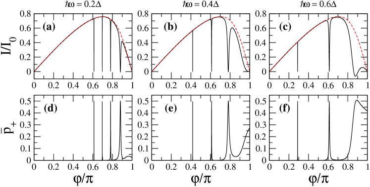
Figure 2: (Color online) (a-c) Zero temperature supercurrent, in units of $I_{0}=e\Delta/\hbar$, as a function of the phase for $\tau=0.95$, $\alpha=0.15$ and three different values of the microwave frequency, as indicated in the upper part of the graphs. The solid lines correspond to the numerical results obtained with the two-level model, while the dashed lines is the result obtained with the adiabatic approximation. (d-f) Time-average occupation of the upper ABS for the cases shown in the upper panels.

In order to have a first impression of the results from this two-level model, we show in Fig. 2 a few examples of the CPR of a highly transmissive channel ($\tau=0.95$) computed with the numerical recipe that we have just described.note-IC The upper panels of this figure show the CPR for a moderate power ($\alpha=0.15$) and three different values of the microwave frequency. For comparison, we also show the result obtained with the adiabatic approximation of Eq. (4). As one can see, the main difference is the appearance in the results of the two-level model of a series of dips at certain values of the phases where the current is largely suppressed. It is easy to understand that such dips are due to microwave-induced transitions between the ABSs. These transitions enhance the population of the upper ABS, which at zero temperature would be empty otherwise, and at the same time they reduce the occupation of the lower ABS. This redistribution of the quasiparticles in turn results in a suppression of the current. The microwave-induced transitions occur with the highest probability when the distance in energy between the ABSs (the Andreev gap) is equal to a multiple of the photon energy, i.e., when $2E_{\rm A}(\varphi)=n\omega$, where $n=1,2,\dots$ is the number of photons involved in the transition. If this condition is expressed in terms of the phase $\varphi$, it adopts the from

$$\varphi_{n}=2\,{\rm arcsin}\sqrt{[1-(n\omega/2\Delta)^{2}]/\tau},\;\;n=1,2,\dots\;.$$ (20)

A detailed analysis shows that this expression reproduces the positions of all the dips appearing in the examples of Fig. 2.

This interpretation of the origin of the dips in the CPR can be corroborated by a direct analysis of the occupations of the ABSs. Following the same numerical recipe, we have also computed the average occupation of the upper ABS, $\bar{p}_{+}$, for the examples shown in the upper panels of Fig. 2. The results can be seen in the lower panels of this figure and, as one can observe, there is a clear one-to-one correspondence between the current dips and the enhancement of the time-averaged population of the upper state. In particular, whenever the upper state reaches a population equal to $1/2$, the current vanishes exactly.

The method described above is not only very convenient for numerical calculations, but it also provides a route to obtain analytical results. In what follows, we show how this method can be used, in particular, to gain a further insight into the microwave-induced supercurrent dips. To proceed, it is useful to first rewrite Eq. (19) in a more convenient form. In particular, we would like to avoid the calculation of eigenvectors in this equation. This can be done by noting that the unperturbed Hamiltonian (8) obeys

$$\hat{\sigma}_{x}\hat{H}_{\rm A}\hat{\sigma}_{x}=-\hat{H}_{\rm A}\;.$$ (21)

Consequently, ${\rm v_{-}}\propto{}\sigma_{x}{\rm v_{+}}$, and the dc current given by Eq. (19) can be written as

$$\bar{I}=-{\rm v}_{+}^{\dagger}\left(\hat{\rho}_{0}-\hat{\sigma}_{x}\hat{\rho}_{0}\hat{\sigma}_{x}\right){\rm v}_{+}\left.\frac{\partial E(\chi)}{\partial\chi}\right|_{\chi=0}\;,$$ (22)

where $\hat{\rho}_{0}=\Psi_{0}\Psi_{0}^{\dagger}$. Using the expression for the change of an eigenvalue due to a perturbation, we can finally write

$$\bar{I}=\left.\frac{\partial E(\chi,\mu)}{\partial\mu}\frac{\partial E(\chi,\mu)}{\partial\chi}\right|_{\chi,\mu=0}\;.$$ (23)

Here $E(\chi,\mu)$ is an eigenvalue of the matrix

$$\hat{M}(\chi,\mu)=\frac{i}{T}\hat{\Omega}(T,\chi)+\mu\left(\hat{\rho}_{0}-\hat{\sigma}_{x}\hat{\rho}_{0}\hat{\sigma}_{x}\right)\;,$$ (24)

$\hat{\Omega}(T,\chi)\equiv{\rm log}[U(T,\chi)]$ and $\mu$ is an additional perturbation parameter. The problem is now reduced to finding the eigenvalues of a 2$\times$2 matrix.

As discussed above, the dc current for weak fields only deviates from the adiabatic result close to the resonant conditions $n\omega=2E_{\rm A}$ (with $n=1,2,3,\ldots$), where the transitions between the ABSs are more likely. In order to study what happens close to these resonant situations, we can consider the problem in a rotating frame, and rewrite the evolution operator $\hat{U}(t)$ defined in Eq. (13) as

$$\hat{U}(t)=e^{-i\hat{W}_{n}t}{\cal T}e^{-i\int_{0}^{t}dt^{\prime}\hat{\tilde{H}}_{n}(t^{\prime})}\equiv e^{-i\hat{W}_{n}t}\hat{\tilde{U}}_{n}(t)\,,$$ (25)

where $\hat{W}_{n}=n\omega\hat{\sigma}_{z}/2$ and the rotating-frame Hamiltonian is

$$\hat{\tilde{H}}_{n}(t)=e^{i\hat{W}_{n}t}[\hat{H}_{\rm A}(t)-\hat{W}_{n}]e^{-i\hat{W}_{n}t}\;.$$ (26)

The generating function can then be written as in Eq. (14) simply by substituting $\hat{H}_{\rm A}$ by $\hat{\tilde{H}}_{n}$. The additional exponential factors simply cancel out, and the Hamiltonian $\hat{\tilde{H}}_{n}(t)$ remains periodic. Thus, we can proceed exactly as above.

The key idea that allows us to obtain analytical results is the fact that for weak fields ($\alpha\ll 1$), the dynamics in the rotating frame are slow ($\hat{\tilde{H}}_{n}$ is small) around the corresponding resonance. For this reason, we can use the Magnus expansionMagnus54 to determine the matrix $\hat{\Omega}$ appearing in Eq. (24):

$$\hat{\Omega}(T)= -i\int_{0}^{T}dt_{1}\hat{H}_{n}(t_{1})$$ (27)

$$-\frac{1}{2}\int_{0}^{T}dt_{1}\int_{0}^{t_{1}}dt_{2}\left[\hat{H}_{n}(t_{1}),\hat{H}_{n}(t_{2})\right]+\ldots\,.$$

This is essentially an expansion in the parameter $\lambda_{n}\sim 2n\pi(E_{\rm A}-n\omega/2)/\omega$, which indeed is small close to a resonance.

We proceed now computing the dc current close to the first resonance $\omega=2E_{\rm A}$, assuming that initially the system is in its ground state $\Psi_{0}^{\dagger}=(0,1)$. We choose $\hat{W}=\omega\sigma_{z}/2$, and take only the first term of the expansion (27), expanding up to the first order in $\alpha$ and $\chi$. The time integral is straightforward to evaluate, and we obtain

$$\frac{i}{T}\hat{\tilde{\Omega}}_{1}(T,\chi) \simeq\bigl{[}E_{\rm A}-\frac{\omega}{2}+2e\chi E_{\rm A}^{\prime}\bigr{]}\hat{\sigma}_{z}$$ (28)

$$+\frac{r}{2E_{\rm A}^{2}}\alpha\bigl{[}(\Delta^{2}-E_{\rm A}^{2})\frac{\omega}{2}-\chi(\Delta^{2}+E_{\rm A}^{2})2eE_{\rm A}^{\prime}\bigr{]}\hat{\sigma}_{x}\,.$$

Note that this expression is analogous with the well-known rotating wave approximation, with the difference that by considering the generating function, our formalism takes the time dependence of the operator $\hat{I}(t)$ into account. For the eigenvalues of the matrix $\hat{\tilde{M}}_{1}=(i/T)\hat{\tilde{\Omega}}_{1}+\mu\sigma_{z}$ we obtain

$$E^{2} =[E_{\rm A}-\frac{\omega}{2}+\mu+2e\chi E_{\rm A}^{\prime}]^{2}$$ (29)

$$+(r\alpha/2E_{\rm A}^{2})^{2}[(\Delta^{2}-E_{\rm A}^{2})\frac{\omega}{2}-\chi(\Delta^{2}+E_{\rm A}^{2})2eE_{\rm A}^{\prime}]^{2}\,.$$

Finally, working in the limit $(\omega-2E_{\rm A})/\Delta\ll 1$ for simplicity, we find the dc current from Eq. (23):

$$\bar{I}_{1}(\varphi,\omega,\alpha)\approx-2eE_{\rm A}^{\prime}\left(1-\frac{\Omega_{r,1}^{2}}{(\omega-\omega_{1})^{2}+\Omega_{r,1}^{2}}\right)\,,$$ (30)

where the resonant frequency $\omega_{1}=2E_{\rm A}$ equals the unperturbed Andreev level spacing $2E_{\rm A}$ (up to first order in $\alpha$), and $\Omega_{r,1}=r\alpha\omega(\Delta^{2}-E_{\rm A}^{2})/2E_{\rm A}^{2}$ is the corresponding Rabi frequency. This expression tells us that the current vanishes exactly at the resonant condition $\omega=\omega_{1}$ and that the width of the current dip is given by $\Omega_{r,1}$, which is linear in $\alpha$. Moreover, its form clearly suggests that the populations of the two states undergo Rabi oscillations with the frequency $\Omega_{r,1}$, as usual in two-state systems, and the time-averaged populations of the ABS coincide at the resonance. As a consequence, the dc current drops to zero at the resonance, a result that qualitatively coincides with the prediction in Ref. Shumeiko1993, .

We can also determine the dc current at the higher resonances, for example for $\omega\approx E_{A}$. In this case we work in the frame corresponding to $\hat{W}_{2}=\omega\hat{\sigma}_{z}$. As the resonance is due to two-photon processes, terms up to order $\alpha^{2}$ must be taken into account, which requires including the first two terms in Eq. (27). The computations are again straightforward, and up to the second order in $\alpha$ we obtain

$$\frac{i}{T}\hat{\tilde{\Omega}}_{2} \approx\bigl{[}E_{\rm A}-\omega+\alpha^{2}E_{\rm A}^{\prime\prime}+2e\chi E_{\rm A}^{\prime}+r^{2}\alpha^{2}\omega\frac{(\Delta^{2}-\epsilon^{2})^{2}}{12E_{\rm A}^{4}}\bigr{]}\hat{\sigma}_{z}$$ (31)

$$-\frac{r\alpha^{2}E_{\rm A}^{\prime}}{2E_{\rm A}^{2}}\bigl{[}\Delta^{2}\bigl{(}\frac{\omega}{E_{\rm A}}+1\bigr{)}-E_{\rm A}^{2})\bigr{]}\hat{\sigma}_{x}\;.$$

For simplicity, we dropped terms of order $\alpha\chi$, which do not essentially affect the form of the resonance. As above, the current is obtained from the eigenvalues of $\hat{\tilde{M}}_{2}=(i/T)\hat{\tilde{\Omega}}_{2}+\mu\sigma_{z}$, and it adopts the form

$$\bar{I}_{2}(\varphi,\omega,\alpha)\simeq-2eE_{\rm A}^{\prime}\left(1-\frac{\Omega_{r,2}^{2}}{(\omega-\omega_{2})^{2}+\Omega_{r,2}^{2}}\right)\,,$$ (32)

where $\omega_{2}=E_{\rm A}+\alpha^{2}E_{\rm A}^{\prime\prime}+r^{2}\alpha^{2}(\Delta^{2}-E_{\rm A}^{2})^{2}/12E_{\rm A}^{3}$ and $\Omega_{r,2}=r\alpha^{2}(2\Delta^{2}-E_{\rm A}^{2})E_{\rm A}^{\prime}/2E_{\rm A}^{2}$. Here, one can observe that the resonant frequency is shifted from the position $2\omega=2E_{\rm A}$ by two contributions: the first arises from nonlinearities, and the second is the Bloch-Siegert shift.Bloch1940

One can also go further and compute the dc current around resonances $n>2$, although this gets progressively more cumbersome as an increasing number of terms are required in the Magnus expansion, reflecting the increasing number of allowed multiphoton processes generated by the nonlinearities. One can however see from Eqs.(30,32), and also check for higher resonances, that the width of the resonances scales with $\alpha^{n}$. Moreover, one can show that within this model, the time-averaged current vanishes exactly at each resonance, i.e., $\bar{I}\rvert_{\omega=\omega_{n}}=0$.

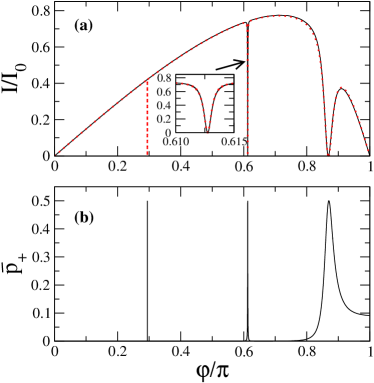
Figure 3: (Color online) (a) Current-phase relation in the two-level model, obtained from Eq. (33) (solid line) and numerics based on Eq. (19) (dotted line). Parameters are $\omega=0.6\Delta$, $\tau=0.95$, and $\alpha=0.05$. The $n=3$ resonance is not included in the analytical approximation. Inset: close-up of the second resonance. (b) Time-averaged population $\bar{p}_{+}$ of the upper Andreev state for the same parameters.

The results Eqs.(30,32) can be combined into a single approximate expression

$$\bar{I}\approx-2eE_{A}^{\prime}\biggl{(}1-\frac{\Omega_{r,1}^{2}}{(\omega-\omega_{1})^{2}+\Omega_{r,1}^{2}}\biggr{)}\biggl{(}1-\frac{\Omega_{r,2}^{2}}{(\omega-\omega_{2})^{2}+\Omega_{r,2}^{2}}\biggr{)}\,.$$ (33)

The quality of this approximation can be established by comparing it with the exact numerical results. This is done in Fig. 3 where we have considered the case of a weak microwave field ($\alpha=0.05$). There is an excellent agreement between Eq. (33) and the numerical results, apart from the fact that the numerics also include a dip produced by three-photon processes, which we have left out from the above approximation.

We can conclude this section by saying that in spite of the simplicity of the two-level model considered here, such a model captures the essential physics of the microwave-irradiated SQPC and, as we show in the next section, it provides accurate results for not too high frequencies and up to moderate radiation power. As we establish in the next section, the limitations of the two-level model are mainly related to the fact that it does not take into account the contribution of the continuum of states outside the gap region.

IV The Keldysh-Green function approach

In the previous section we have analyzed the supercurrent assuming that the only contribution comes from the ABSs. While this is true for a SQPC in equilibrium, it is not obvious that this should be the case in the presence of a microwave field. Indeed, at high frequencies or at high radiation powers, and especially at finite temperatures, transitions between the ABSs and the continuum of states outside the gap become possible and, in principle, they can also contribute to the current. Therefore, in order to describe the complete phenomenology of irradiated SQPCs we must develop a fully microscopic theory. This is the goal of this section.

Our microscopic theory is based on the Keldysh-Green function approach. In this approach the starting point is the expression for the quasiclassical Green functions of the left (L) and right (R) electrodes. In our case, these Green functions can be expressed in terms of the equilibrium Green functions $\check{g}(t-t^{\prime})$ as

$$\check{G}_{R(L)}(t,t^{\prime})=e^{\pm i\phi(t)\hat{\tau}_{3}/2}\check{g}(t-t^{\prime})e^{\mp i\phi(t^{\prime})\tau_{3}/2}\;.$$ (34)

Here $\phi(t)$ is the time-dependent phase given by Eq. (2) and the upper (lower) sign in the exponents corresponds to the R (L) electrode. The symbol $\check{\,}$ indicates that the Green functions are 4$\times$4 matrices in the Keldysh-Nambu space, where they have the structure

$$\check{G}=\begin{pmatrix}\hat{G}^{R}&\hat{G}^{K}\\ 0&\hat{G}^{A}\end{pmatrix}\;.$$ (35)

Here the symbol $\hat{\,}$ indicates that the different elements are 2$\times$2 Nambu matrices. The retarded (R), advanced (A) and Keldysh (K) components of the equilibrium Green functions appearing in Eq. (34) are given by

$$\check{g}(t)=\int^{\infty}_{-\infty}\frac{dE}{2\pi}e^{-iEt/\hbar}\check{g}(E),$$ (36)

where

$$\hat{g}^{R(A)}(E) = g^{R(A)}(E)\hat{\tau}_{3}+f^{R(A)}(E)i\hat{\tau}_{2}$$ (37)

$$\hat{g}^{K}(E) = \left[\hat{g}^{R}(E)-\hat{g}^{A}(E)\right]\tanh(E/2k_{\rm B}T)$$ (38)

and

$$g^{R(A)}(E)=\frac{E}{\sqrt{(E\pm i\eta)^{2}-\Delta^{2}}}=\frac{E}{\Delta}f^{R(A)}(E),$$ (39)

where $\eta$ describes the inelastic scattering energy rate within the relaxation time approximation and $T$ is the temperature.

Different authors have shown that the transport properties of a point contact with an arbitrary time-dependent voltage can be described by making use of adequate boundary conditions for the full quasiclassical propagators.Zaitsev1998 ; Nazarov1999 ; Cuevas2001 ; Kopu2004 These boundary conditions can be expressed in terms of a current matrix

$$\check{I}=\left(\begin{array}[]{ccc}\hat{I}^{R}&\hat{I}^{K}\\ 0&\hat{I}^{A}\end{array}\right),$$ (40)

which for the case of a single-channel SQPC of transmission $\tau$ can be expressed in terms of the lead Green functions of Eq. (34) asNazarov1999

$$\check{I}(t,t^{\prime})=2\tau\left[\check{G}_{L},\check{G}_{R}\right]_{\circ}\circ\left[4-\tau\left(2-\left\{\check{G}_{L},\check{G}_{R}\right\}_{\circ}\right)\right]^{-1}(t,t^{\prime}).$$ (41)

Here, the symbol $\circ$ denotes the convolution over intermediate time arguments. Finally, the electric current is obtained by taking the trace

$$I(t)=\frac{e}{4\hbar}{\rm Tr}\hat{\tau}_{3}\hat{I}^{K}(t,t)\;,$$ (42)

where $\hat{\tau}_{3}$ is the third Pauli matrix in Nambu space.

Due to the periodic time dependence of the phase [Eq. (2)], the Green functions $\check{G}_{L(R)}$, and any products of them, admit the following Fourier expansion

$$\check{G}(t,t^{\prime})=\sum^{\infty}_{m=-\infty}e^{im\omega t^{\prime}}\int\frac{dE}{2\pi}e^{-iE(t-t^{\prime})/\hbar}\check{G}_{0m}(E),$$ (43)

where $\check{G}_{nm}(E)\equiv\check{G}(E+n\hbar\omega,E+m\hbar\omega)$ are the corresponding Fourier components in energy space, and $n,m$ are integers. In particular, the Fourier components of $\check{G}_{L(R)}$ can be deduced from Eq. (34). For instance, for the left electrode, $\check{G}_{nm}(E)$ is given by

$$(\check{G}_{L})_{nm}=\sum_{l}\check{\Gamma}_{nl}\check{g}_{l}\check{\Gamma}^{*}_{lm},$$ (44)

where

$$\check{\Gamma}_{nm}=\left(\begin{array}[]{cc}\hat{\Gamma}_{nm}&0\\ 0&\hat{\Gamma}_{nm}\end{array}\right),\hat{\Gamma}_{nm}=\left(\begin{array}[]{cc}{\cal P}_{nm}&0\\ 0&{\cal P}^{\ast}_{nm}\end{array}\right).$$ (45)

Here, ${\cal P}_{nm}=(i)^{m-n}J_{m-n}(\alpha/2)e^{i\varphi/4}$, where $J_{n}$ is the Bessel function of order $n$, and $\check{g}_{n}=\check{g}(E+n\hbar\omega)$ is the equilibrium Green function matrix with the argument shifted in energy.

From this discussion, it is easy to understand that the current adopts the general expression

$$I(t)=\sum^{\infty}_{m=-\infty}I_{m}e^{im\omega t},$$ (46)

which means that the current oscillates in time with the microwave frequency and all its harmonics. These current components can be computed from the Fourier components in energy space of $\check{I}$ in Eq. (41). From that equation, it is straightforward to show that the Fourier components of $\hat{I}^{K}$ are given by

$$\hat{I}_{nm}^{K}=\sum_{l}[\hat{A}_{nl}^{R}\hat{X}_{lm}^{K}+\hat{A}_{nl}^{K}\hat{X}_{lm}^{A}].$$ (47)

Here, we have defined the matrices $\check{A}_{nm}\equiv 2\tau[\check{G}_{L},\check{G}_{R}]_{nm}$ and $\check{X}_{nm}=[4\check{1}-\tau(2-\{\check{G}_{L},\check{G}_{R}\})]^{-1}_{nm}$, which can be determined from the Fourier components of $\check{G}_{L(R)}$. Once the components of $\hat{I}^{K}$ are obtained from Eq. (47), one can compute the current. We are only interested here in the dc component, which reads

$$I(\varphi,\omega,\alpha)=\frac{e}{4\hbar}\int\frac{dE}{2\pi}{\rm Tr}\hat{\tau}_{3}\hat{I}^{K}_{00}(E,\varphi,\omega,\alpha).$$ (48)

The dc current can be calculated analytically in certain limiting cases: for example in the absence of microwaves, where it reduces to Eq. (3), in the tunnel regime or for very weak fields. However, for arbitrary radiation power one needs to evaluate Eq. (48) numerically. In the next subsections we present the results for the dc current of this microscopic theory and we compare them with those obtained from the two-level model of Section III.

IV.1 Zero-temperature limit: Comparison with the two-level model

We focus first on the analysis of the results of the exact theory at zero temperature. This allows us, in particular, to make a comparison with the two-level model of Section III and to establish its range of validity.

In Fig. 4 we show several examples of the CPR calculated with the microscopic approach (solid lines) for a highly conductive channel ($\tau=0.95$) for several frequencies and low values of the radiation power ($\alpha\ll 1$). For comparison, we also show the results of both the two-level model (dashed lines) and the adiabatic approximation (dotted lines). As one can see, the main deviation from the adiabatic results is the appearance of a series of dips, as discussed in section III. These features, which originate from the microwave-induced transitions between the ABSs, are accurately reproduced by the two-level model (both the position and the width of the dips). There is a small discrepancy between the exact result and those of the two-level model for phases close to $\pi$, i.e., when the level spacing between the ABS is very small. This is understandable since the model assumes that $\hbar\dot{\phi}(t)\ll 2E_{\rm A}$, which is not fulfilled when $\varphi\sim\pi$ and $\tau$ is close to 1. Notice also that for the high-order dips (due to high-order photonic processes), the suppression of the current in the two-level model is larger than in the case of the exact theory. The reason is the additional broadening introduced by the finite inelastic scattering rate used in the calculations with the microscopic theory, which in this case is $\eta=10^{-4}\Delta$.

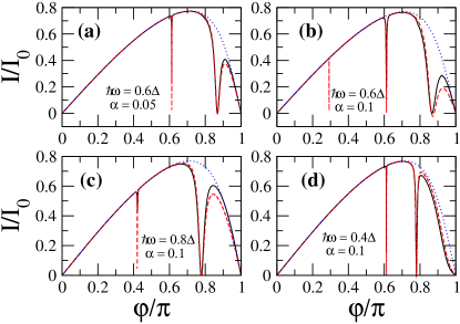
Figure 4: (Color online) Four examples of the zero-temperature current-phase relation for $\tau=0.95$ obtained from the microscopic model (solid lines), the two level model (dashed lines) and the adiabatic approximation (dotted lines). The parameters characterizing the microwave field are indicated in the different panels.

The good agreement between the microscopic theory and the two-level model in these examples can be understood as follows. At zero temperature, the lower ABS is fully occupied, while the upper one is empty. Therefore, for small values of $\alpha$ and $\hbar\omega<\Delta$ transfer of quasiparticles between the continuum and the ABSs is not possible. The agreement between these models is further confirmed in Fig. 5(a), where the CPR is shown for $\hbar\omega=0.6\Delta$, $\alpha=0.1$ and two lower values of the transmission ($\tau=0.6$ and $0.8$). In this case, the agreement is almost perfect for all phases. The reason is that now the smallest energy gap between the ABSs, which occurs at $\varphi=\pi$, is large enough to avoid the overlap of the levels in the presence of the microwave field. If the transmission is further reduced, no transitions can occur between the Andreev states and the adiabatic approximation becomes exact.

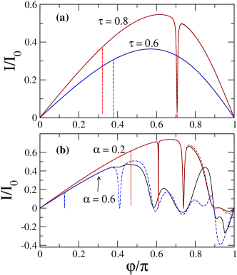
Figure 5: (Color online) (a) The current-phase relation for $\alpha=0.1$, $\hbar\omega=0.6\Delta$ and two values of the transmission coefficient, $\tau=0.8$ and $\tau=0.6$. (b) The current-phase relation for $\hbar\omega=0.3\Delta$, $\tau=0.95$ and two values of $\alpha$, 0.2 and 0.6. In both panels the solid lines correspond to the microscopic theory and the dashed lines to the two-level model.

From the discussion above, we can conclude that the two-level model provides an excellent description of the supercurrent at zero temperature and for weak fields ($\alpha\ll 1$). However, as the radiation power increases, the situation changes. This is illustrated in Fig. 5(b), where we show the CPR for a highly conductive channel ($\tau=0.95$), a frequency $\hbar\omega=0.3\Delta$ and two values of $\alpha$. As one can see, the deviations between the results of the two-level model and the microscopic theory become more apparent as the power increases. The main reason for this discrepancy is the occurrence of multiphotonic processes, which become more probable as the power increases. These processes induce quasiparticle transitions between the ABSs and the continuum part of the energy spectrum, which are not included in the two-level model.

As one could already see in Fig. 5(b), as the radiation power increases the supercurrent dips broaden and the CPR acquires a very rich structure. We illustrate this fact in more detail in Fig. 6 where we show the evolution of the CPR with $\alpha$ for two values of the transmission (0.95 and 0.8) and for frequency $\hbar\omega=0.3\Delta$. Notice that as the power increases, the dips disappear, the CPRs become highly non-sinusoidal, and in some regions of the phase the current can reverse its sign. These results are clearly at variance with those found within the adiabatic approximation (see Section II). They are a consequence of a complex interplay between the dynamics of the ABSs, which are broadened by the coupling to the microwaves, and the multiple transitions induced between the ABSs and the continuum of states. This very rich behavior has also important implications for the critical current, which for high transmission strongly deviates from the standard behavior described by the adiabatic approximation. This is discussed below in detail. Finally, it is worth stressing that the values of $\alpha$ used in Fig. 6 are easily achievable in experiment, as demonstrated in the context of atomic contacts,Chauvin2006 semiconductor nanowiresDoh2005 or graphene junctions.Heersche2007 ; Du2008 ; Jeong2011 Therefore, these results indicate that the microscopic theory presented here will always be necessary for the description of the experimental results of highly transmissive junctions at sufficiently high power, no matter how low the microwave frequency is.

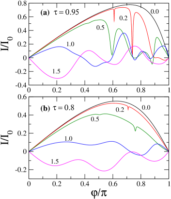
Figure 6: (Color online) The zero-temperature current-phase relation for $\hbar\omega=0.3\Delta$ and two values of the transmission: (a) $\tau=0.95$ and (b) $\tau=0.8$. The different curves correspond to different values of $\alpha$, as indicated in the graphs. The inelastic broadening used in these calculations is $\eta=10^{-3}\Delta$.

IV.2 Finite temperature: Enhancement of the supercurrent

We now turn to the analysis of the supercurrent at finite temperature, carried out within the microscopic model. The new ingredient at finite temperature is the fact that the ABSs are neither fully occupied nor fully empty, which means that quasiparticle transitions between the continuum of states and the bound states are possible, even for frequencies $\hbar\omega<\Delta$. This has important consequences.

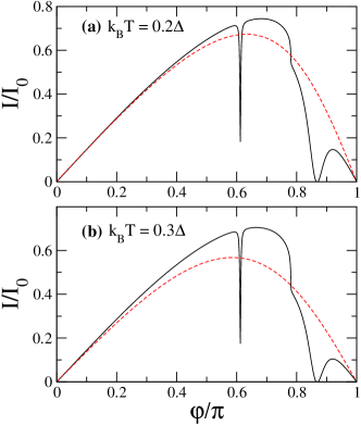
Figure 7: (Color online) The current-phase relation for $\hbar\omega=0.6\Delta$, $\alpha=0.1$, $\tau=0.95$ and two different temperatures: (a) $k_{B}T=0.2\Delta$ and (b) $k_{B}T=0.3\Delta$. The solid lines in both panels correspond to the results of the microscopic theory and the dashed lines to the supercurrent in the absence of microwaves ($\alpha=0$).

In Fig. 7 we show the CPR for $\hbar\omega=0.6\Delta$, $\alpha=0.1$, $\tau=0.95$ and two different temperatures. For comparison, we also show the results in the absence of microwaves (dashed lines). Apart from the dips, whose origin is discussed above in detail, one can observe that at a certain value of the phase ($\varphi_{0}\approx 0.78\pi$) the current is suppressed. Notice that the suppression is stronger as the temperature increases. Moreover, for phases smaller than $\varphi_{0}$ the supercurrent exceeds its value in the absence of microwaves. In other words, for $\varphi<\varphi_{0}$ there is an enhancement of the supercurrent induced by the microwave field. The origin of this enhancement is the promotion of quasiparticles from the continuum below $-\Delta$ to the lower ABS by the microwave field. There is also an identical contribution coming from transitions connecting the upper state and the continuum above $+\Delta$. At low microwave powers, these processes can only occur if the field frequency is larger than the distance in energy between the gap edges and the nearest ABS, i.e., if $\hbar\omega>\Delta-E_{\rm A}(\varphi)$, and they become possible at finite temperature because the lower state is not fully occupied and the upper state is not fully empty. For the parameters of Fig. 7 the previous condition is satisfied if $E_{\rm A}(\varphi)>0.4\Delta$, which corresponds to a phase $\varphi<0.78\pi$. Obviously, this phenomenon of microwave-enhanced supercurrent cannot be described by the two-level model since this models ignores the contribution of the continuum part of the spectrum.

In order to confirm our interpretation of the origin of the microwave-enhanced supercurrent, we have derived analytical results describing this phenomenon in the limit of weak microwave fields. We have obtained such results with the help of an alternative method, known as Hamiltonian approach, which for SQPCs has been shown to be equivalent to the microscopic theory described at the beginning of this section.Cuevas1996 ; Cuevas2001 ; Bergeret2005 In this approach, a point contact is described in terms of a tight-binding-like Hamiltonian and the transport properties are calculated following a perturbative approach, where the coupling between the electrodes is treated as the perturbation. Although the calculations with this method are slightly more cumbersome than with the approach used above, it has certain advantages. For instance, it also allows us to obtain the density of states (DOS) at the contact. Moreover, a perturbative analysis (in the field) is much simpler when using Eq. (48). The technical details of the Hamiltonian approach are described in the Appendix A, and in what follows, we only discuss the results of this analysis.

We are interested in the correction to the current due to the microwave field which is responsible for the enhancement of the supercurrent. Thus, based on our numerical results, we explore the parameter region where $\Delta-E_{A}<\hbar\omega$. Moreover, in order to avoid the resonant transitions between the ABSs, we also assume that $\hbar\omega<2E_{A}$. As described in Appendix A, a perturbative analysis to lowest order in the parameter $\alpha$ shows that the supercurrent can be written as

$$I(\varphi)=I_{\rm eq}(\varphi)+\delta I(\varphi),$$ (49)

where $I_{\rm eq}$ is the equilibrium supercurrent given by Eq. (3), and the correction $\delta I$ contains several contributions of order $\alpha^{2}$. There are two types of contributions. One type of contribution is related to the change in the bound states induced by the coupling to the electromagnetic field. The other contribution comes from the modification of the occupations of the bound states due to the quasiparticle transitions involving the ABSs. In the range of parameters that we are interested in, the second type of contributions dominates at high enough temperatures and, in particular, they are responsible for the supercurrent enhancement. Those contributions can be written in the spirit of Eq. (3) as

$$\delta I_{\rm enh}(\varphi)=I^{-}_{\rm A}(\varphi)\delta n^{-}(\varphi)+I^{+}_{\rm A}(\varphi)\delta n^{+}(\varphi),$$ (50)

where $I^{\pm}_{\rm A}(\varphi)=(2e/\hbar)\partial E^{\pm}_{\rm A}/\partial\varphi$ give the contribution of the states to the equilibrium supercurrent, and $\delta n^{\pm}(\varphi)$ are the corrections to the occupations of the ABSs due to the application of the microwave field. These corrections can be written as

$$\delta n^{\pm}(\varphi) = \frac{\alpha^{2}\tau}{8}\left[{\rm Re}\left\{e^{i\varphi}\rho_{L}(E^{\pm}_{\rm A})\tilde{\rho}_{R}(E^{\pm}_{\rm A}\pm\omega)\right\}+\right.$$ (51)

$$\left.\nu(E^{\pm}_{\rm A})\nu(E^{\pm}_{\rm A}\pm\omega)\right][F_{0}-F_{\pm 1}].$$

Here, $F_{n}$ is the distribution function with shifted arguments $F_{n}=\tanh[(E+n\hbar\omega)/2k_{\rm B}T]$, $\nu(E)$ is the density of states at the contact in the absence of microwaves, and $\rho_{j}$ and $\tilde{\rho}_{j}$ are the real part of the anomalous Green functions on the left (L) and (R) side of the interface ($j=L,R$) without the field, as defined in Appendix A. Equation (51) has a very appealing form and it tells us that the occupations of the ABSs can be changed by microwave-induced transitions connecting these states between the continua below and above the gap. These transitions are illustrated in Fig. 8, where we also present an example of the density of states of the contact in the absence of microwaves, $\nu(E)$. This density of states is given by (see Appendix A)

$$\nu(E)={\rm Re}\left\{\frac{E\sqrt{(E+i\eta)^{2}-\Delta^{2}}}{(E+i\eta)^{2}-E_{\rm A}^{2}}\right\}\;,$$ (52)

where the poles correspond to the ABSs and, as one can see in Fig. 8, there are no singularities at the gap edges $E=\pm\Delta$.

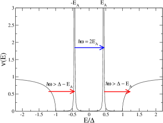
Figure 8: (Color online) The local density of states at the contact in the absence of microwaves, as defined in Eq. (52), as a function of energy for $\tau=0.95$, $\varphi=3\pi/4$ and $\eta=10^{-3}\Delta$. The lower arrows represent the microwave-induced transitions between the continuum part of the spectrum and the Andreev bound states which are responsible for the supercurrent enhancement at finite temperatures. The upper arrow indicates the resonant transition between the ABSs, which suppresses the supercurrent.

From Eq. (51) one can show that the transitions between the continuum of states below $-\Delta$ and the lower ABS increase the population of the lower state ($\delta n^{-}>0$), while the photon processes connecting the continuum above $+\Delta$ and the upper ABS decrease the occupation of the upper state ($\delta n^{+}<0$). As one can see from Eq. (50), both types of processes give a positive contribution to the current at finite temperatures and thus, they are responsible for the supercurrent enhancement. Indeed, due to the electron-hole symmetry of this problem, terms in Eq. (50) give the same contribution to the current. Finally, the correction to the current due to these microwave-induced transitions involving the continuum can be written as

$$\delta I_{\rm enh}(\varphi) = \alpha^{2}\left(\frac{-2eE^{\prime}_{\rm A}}{\hbar}\right)\frac{\tau}{16}\times$$

$$\frac{\sqrt{(E_{\rm A}+\hbar\omega)^{2}-\Delta^{2}}\sqrt{\Delta^{2}-E_{\rm A}^{2}}}{\eta\hbar\omega E_{\rm A}(2E_{\rm A}+\hbar\omega)}\times$$

$$\left[E_{\rm A}\hbar\omega+\Delta^{2}(1+\cos\varphi)\right]\left[F_{1}-F_{0}\right]\Theta\left(|E_{\rm A}+\hbar\omega|-\Delta\right).$$

This expression gives a positive contribution to the supercurrent and it explicitly shows that the enhancement can only take place when $\hbar\omega>\Delta-E_{\rm A}$. According to Eq. (IV.2), the correction to the current is proportional $1/\eta$, the inelastic scattering time. In our model the parameter $\eta$ describes the energy loss mechanism via which the microwave power is dissipated. For simplicity, we assume it to be energy and frequency independent. Equation (IV.2) reproduces the exact results obtained with the microscopic approach in the limit of weak fields and in the range of frequencies where the transitions between the ABSs cannot take place. This is illustrated in Fig. 9 where we show the supercurrent for a fixed value of the phase ($\varphi=\pi/2$) as a function of the frequency for $\tau=0.95$, $\alpha=0.1$ and $k_{\rm B}T=0.4\Delta$. As one can see, the exact result (solid line) remains constant for low frequencies. Then, at $\hbar\omega=\Delta-E_{\rm A}$ there is a rise of the supercurrent due to the onset of the transitions connecting the ABSs with the continuum of states. This increase of the supercurrent is well described by the analytical result of Eq. (IV.2) (dashed line). At higher frequencies, one can observe the dips due to the transitions between the ABSs. The dip at $\hbar\omega=E_{\rm A}$ corresponds to a two-photon process, while the one at $\hbar\omega=2E_{\rm A}$ is produced by a single-photon process. Finally, at $\hbar\omega=\Delta+E_{\rm A}$ the supercurrent starts to decrease due to microwave-induced transitions between the continuum below $-\Delta$ and the upper ABS and similar ones between the continuum above $+\Delta$ and the lower ABS. These transitions, which can also occur at zero temperature, tend to increase the occupation of the upper state and to reduce the population of the lower one, which results in a reduction of the net supercurrent.

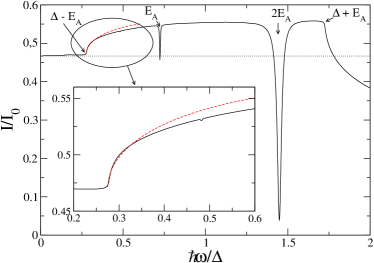
Figure 9: (Color online) The dc Josephson current as a function of the frequency $\omega$ of the microwave field for a fixed value of the phase $\varphi=\pi/2$, and $\alpha=0.1$, $\tau=0.95$ and $k_{B}T=0.4\Delta$. The solid line shows the exact numerical result while the dashed line shows the result obtained from Eq. (IV.2). The dotted line shows the value of the current in the absence of the microwave field.

As one can see in Fig. 7 and  9, the maximum supercurrent sustained by the junction, i.e. the critical current, can also be enhanced by the microwave field at finite temperatures. A microwave-enhanced critical current was first reported in experiments on superconducting microbridgesWyatt1966 ; Dayem1967 and explained by EliashbergEliashberg1970 in 1970 in terms of the stimulation of the superconductivity in the electrodes, which were made of thin films. Such a stimulation, and the corresponding microwave-enhanced critical current, only occur at temperatures very close to the critical temperature. Enhancements at much lower temperatures were reported in the 1970’s in the context of SNS structures,Notarys1973 ; Warlaumont1979 and they have been recently explained in terms of the redistribution of the quasiparticles induced by the field.Virtanen2010 In this case, for the enhancement to occur, the temperature must be of the order of the minigap in the normal wire, which can be much lower than the critical temperature of the superconducting leads.

As discussed above, in the case of a point contact the mechanism is similar to that of diffusive SNS structures,Virtanen2010 but it involves discrete ABSs, rather than a continuous band of ABSs, as in the case of diffusive proximity structures. For this reason we may expect the enhancement of the critical current in SQPCs to occur at intermediate temperatures, when $k_{\rm B}T$ is of the order of the energy distance between the ABSs and the gap edges ($\Delta-E_{\rm A}(\varphi_{\rm max})$), where $\varphi_{\rm max}$ is the phase value at which the supercurrent reaches its maximum. This is illustrated in Fig. 10, where we show the critical current as a function of $\alpha$ for different temperatures and different values of the transmission. Panel (a) shows the critical current for a highly transmissive channel ($\tau=0.97$) and three values of the temperature. Notice first that at finite temperatures, the critical current at finite $\alpha$ ($\alpha\lesssim 0.5$) exceeds the value in the absence of microwaves ($\alpha=0$). Notice also that as $\alpha$ increases, the critical currents clearly deviate from the behavior described by the adiabatic approximation, which is shown as dashed lines. It is also important to emphasize that the microwave-enhancement of the critical current is not exclusive of high conductive channels and it persists up to relatively low transmissions, as we show in Fig. 10(b-c). The relative enhancement of the critical current is larger the larger is the temperature. It is also worth remarking that at sufficiently high power, the critical current depends only weakly on the temperature.

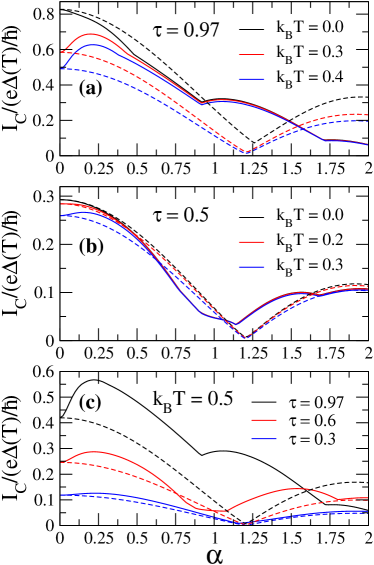
Figure 10: (Color online) The critical current as a function of $\alpha$ for $\hbar\omega=0.6\Delta$. The different curves correspond to different values of the temperature and the transmission as indicated in the graphs. The solid lines correspond to the exact results, while the dashed lines show the results of the adiabatic approximation. In the three panels the critical current has been normalized by $e\Delta(T)/\hbar$, where $\Delta(T)$ is the gap at the corresponding temperature.

V Conclusions and further discussions

Summarizing, we have presented a theoretical analysis of the supercurrent in a phase-biased SQPC under microwave irradiation. We have shown that if the microwave frequency $\omega$ is not high enough to induce transitions between the ABSs or between the ABSs and the continuum of states outside the gap region, the supercurrent is correctly described by the standard adiabatic approximation (see Section II). However, when $\hbar\omega$ is comparable to the Andreev gap (energy distance between the ABSs), quasiparticle transitions between the ABSs can occur and the supercurrent can be largely suppressed at the corresponding values of the phase difference. We have shown that this phenomenon can be nicely explained within a two-level model that describes the dynamics of the ABSs.Zazunov2003 This model indicates that the supercurrent suppression is due to the enhancement of the occupation of the upper ABS induced by resonant transitions from the lower state. Moreover, at low temperatures and weak fields, this model is quantitatively correct provided that (i) the microwave frequency is not high enough to induce transitions connecting the ABSs and the continuum of states, and (ii) the Andreev gap is large compared to the broadening acquired by the ABSs by means of the coupling to the electromagnetic field. Finally, we have shown that whenever microwave-induced transitions between the ABSs and the continuum of states become possible (due to finite temperatures, high frequencies or high radiation powers), a fully microscopic theory is needed to describe the supercurrent. We have developed such a theory and predicted the following effects. First, at finite temperatures it is possible to enhance both the supercurrent and the critical current by the application of a microwave field. This effect originates from the quasiparticle transitions between the ABSs and the continuum of states, which increase the occupation of the lower Andreev state and reduce the population of the upper one. Second, the current-phase relation at high powers is strongly distorted and it can become highly non-sinusoidal exhibiting sign changes in the region between $0$ and $\pi$. Third, the critical current as a function of the radiation power can exhibit large deviations from the standard Bessel-function behavior described by the adiabatic approximation.

It is now pertinent to discuss the connection with experiments. As explained in the introduction, most of the experimental results of the effect of microwaves on the supercurrent of a point contact have been successfully described in the frame of the adiabatic approximation. The reason is that the typical frequency used in the experiments is relatively low ($\hbar\omega\ll\Delta$) and no transitions between the ABSs can occur. However, it is important to remark that there are no fundamental limitations to study the parameter regime where we predict the occurrence of novel effects like the appearance of supercurrent dips in the current-phase relation or the microwave-enhanced critical current. These effects are easier to observe in highly transmissive point contacts where the Andreev gap can become relatively small (much smaller than $\Delta$). The ideal experimental system where to test our predictions is a superconducting atomic contact for several reasons. First, these contacts can sustain a reduced number of channels, which facilitates the comparison with the theory. Second, it has been shown that it is possible to determine independently the set of transmission eigenvalues $\{\tau_{i}\}$,Scheer1997 which has allowed to establish a comparison between theory and experiment with no adjustable parameters for many different transport properties.Cron2001 ; Chauvin2006 ; Rocca2007 . Third, it is possible to tune, at least to a certain extent, the transmission coefficients and, in particular, to achieve very high transmission coefficients, as demonstrated in the context of Al atomic contacts.Scheer1997 ; Chauvin2006 ; Rocca2007 Finally, it has already been shown that in these systems the current-phase relation is amenable to measurements,Rocca2007 and investigations of the transport properties of superconducting atomic contacts under microwave irradiation have already been performed.Chauvin2006 ; note-exp

In experiments with superconducting atomic junctions, even at the level of a single-atom contact, one often has the contribution of several conduction channels. In this sense, one may wonder whether the presence of low-transmissive channels can mask some of the striking effects that we have discussed above. In Fig. 11 we show the CPR for a contact consisting of three conducting channels with transmissions $\tau=0.17,0.6,0.97$ respectively. The current is obtained by adding the contribution of each channel according to Eq. (41). As one can see in Fig. 11 the total current still shows the dips at the resonances corresponding to the channel with the highest transmission ($\tau=0.97$). However, the current does not vanish completely due to the contribution of the low-transmissive channels.

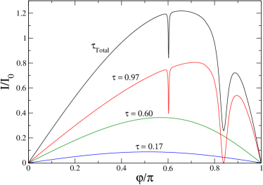
Figure 11: (Color online) The zero-temperature current-phase relation for a point-contact consisting of three channels with transmissions $\tau=0.17,0.6,0.97$, for $\alpha=0.1$ and $\hbar\omega=0.6\Delta$. The dashed lines show the contribution of each channel, while the solid line corresponds to the total current.

It is worth stressing that the major problem to establish a direct comparison between our theory and the experiments is the fact that we have assumed a phase-biased junction. In reality, and depending on the details of the electromagnetic environment seen by the point contact, the phase across the junction may undergo fluctuations (both classical and quantum) which can affect the value of the critical current or the shape of the current-phase relation. Thus, a quantitative comparison with the experiments may require in some cases to combine our theory with a description of the phase fluctuations. For classical fluctuations, this could be done in the spirit of Ref. Chauvin2007, by means of an extension of the resistively shunted junction using our microscopic current-phase relation as a starting point.

Let us conclude by saying that in this work we have shown that the application of microwaves to one of the simplest superconducting systems, namely a SQPC, leads to a very rich phenomenology, which has remained largely unexplored. In particular, we have shown that a microwave field is an ideal tool to make a direct spectroscopy of the Andreev bound states of a superconducting junction. The ideas put forward in this work pave the way for the understanding of the influence of a microwave field on the supercurrent of variety of highly transmissive superconducting weak links.

Appendix A Hamiltonian approach

The transport properties of a microwave-irradiated SQPC can also be described within the so-called Hamiltonian approach.Cuevas1996 ; Cuevas2002 We explain in this appendix how this approach can be used to obtain analytical results for the supercurrent enhancement discussed in Section IV.2. In this approach a single-channel SQPC can be described in terms of the following tight-binding-like Hamiltonian

$$\hat{H}=\hat{H}_{L}+\hat{H}_{R}+\sum_{\sigma}\left\{t\hat{c}^{\dagger}_{L\sigma}\hat{c}_{R\sigma}+t^{\ast}c^{\dagger}_{R\sigma}\hat{c}_{L\sigma}\right\},$$ (54)

where $\hat{H}_{L,R}$ are the BCS Hamiltonians describing the left (L) and right (R) electrodes and the last term describes the coupling between the electrodes. In this last term, $t$ is a hopping element that determines the transmission of the contact.

In this model the current evaluated at the interface between the two electrodes adopts the form

$$I(t)=\frac{ie}{\hbar}\sum_{\sigma}\left\{t\langle c^{\dagger}_{L\sigma}\hat{c}_{R\sigma}\rangle-t^{\ast}\langle c^{\dagger}_{R\sigma}\hat{c}_{L\sigma}\rangle\right\}.$$ (55)

This expression can be rewritten in terms of the Keldysh Green functions as

$$I(t)=\frac{e}{\hbar}{\rm Tr}\bigl{[}\hat{\tau}_{3}\bigl{(}\hat{t}\hat{\cal G}_{RL}^{K}-\hat{t}^{\dagger}\hat{\cal G}_{LR}^{K}\bigr{)}\bigr{]}(t,t)\;.$$ (56)

Here $\hat{\tau}_{3}$ is the corresponding Pauli matrix, Tr denotes the trace in Nambu space, and $\hat{t}$ is the hopping matrix in Nambu space given by

$$\hat{t}=\left(\begin{array}[]{cc}te^{i\phi(t)/2}&0\\ 0&-t^{\ast}e^{-i\phi(t)/2}\end{array}\right).$$ (57)

Here, $\phi(t)$ is the time-dependent superconducting phase given by Eq. (2).

In order to determine the Green functions appearing in the current expression, we follow a perturbative scheme and treat the coupling term in Hamiltonian (54) as a perturbation. The unperturbed Green functions describe the uncoupled electrodes in equilibrium. Thus for instance, the retarded and advanced functions are given by

$$\hat{g}_{jj}^{R(A)}(E)=\frac{-i}{W}\frac{1}{\zeta^{R(A)}(E)}\begin{pmatrix}E&\Delta\\ \Delta&E\end{pmatrix}\;,$$ (58)

where $j=L,R$, $\zeta^{R(A)}=\sqrt{(E+i\eta)^{2}-\Delta^{2}}$, and $W$ is an energy scale related to the normal density of states at the Fermi energy. The full Green functions can then be determined by solving a Dyson equation, where the retarded and advanced self-energies are simply given by the hopping matrix of Eq. (57).

Since we are interested in the limit of weak fields ($\alpha\ll 1$), we can expand the phase factors in Eq. (57) as follows

$$e^{i\phi(t)/2}\approx e^{i\varphi/2}\left(1+\alpha\cos\omega t+\frac{1}{2}\alpha^{2}(\cos\omega t)^{2}+\cdots\right).$$ (59)

Moreover, for the perturbative treatment in $\alpha$ it is convenient to use the full Green functions of the contact in the absence of microwaves ($\alpha=0$), $\hat{G}_{ij}$. It is straightforward to show that these functions can be expressed as

$$\hat{G}_{LL}^{R(A)}=\frac{-i\zeta^{R(A)}}{W(1+\beta)\xi^{R(A)}}\begin{pmatrix}E\pm i\eta&E_{g}^{*}\\ E_{g}&E\pm i\eta\end{pmatrix}\;$$ (60)

$$\hat{G}_{RL}^{R(A)}=\frac{-t}{W^{2}(1+\beta)\xi^{R(A)}}\begin{pmatrix}a^{R(A)}&b^{R(A)}\\ -b^{R(A)*}&-a^{R(A)*}\end{pmatrix}\;,$$ (61)

where $E_{g}=\Delta(1+\beta e^{i\varphi})(1+\beta)$, $\beta=(t/W)^{2}$, $\xi=E^{2}-E_{A}^{2}$, $a=E^{2}e^{-i\varphi/2}-\Delta E_{g}^{*}e^{i\varphi/2}$ and $b=E(E_{g}e^{-i\varphi/2}-\Delta e^{i\varphi/2})$. Similar expressions hold for $G_{RR}$ and $G_{LR}$. These Green functions are now the zero-order propagators of the perturbation theory. Substituting these functions in the current expression of Eq. (56) and identifying the transmission coefficient as $\tau=4\beta/(1+\beta)^{2}$,Cuevas1996 one obtains the expression for the equilibrium current of Eq. (3). On the other hand, from the previous expressions one can determine the local density of states at the contact in the absence of microwaves, which is defined as $\nu_{j}(E)=W(1+\beta)(i/2)(\hat{G}_{jj}^{R}-\hat{G}_{jj}^{A})_{11}$ ($\nu_{L}=\nu_{R}$ in our symmetric contacts). This density of states is given by Eq. (52) and it is shown in Fig. 8.

Going into the energy representation as done in Section IV, the first correction to the current of Eq. (56), which is of order $\alpha^{2}$, contains the following three terms

$$\delta I=\frac{e}{\hbar}\int\frac{dE}{2\pi}{\rm Tr}\bigl{[}\hat{t}^{(2)}\hat{\cal G}_{RL}^{(0)}+\hat{t}^{(0)}\hat{\cal G}_{RL}^{(2)}+\hat{t}^{(1)}\hat{\cal G}_{RL}^{(1)}\bigr{]}-L\leftrightarrow R\,,$$ (62)

where the superindices denote the order of perturbation in $\alpha$. To obtain a complete analytical expression for an arbitrary value of the field frequency is quite cumbersome. Instead, we concentrate on the parameter range where the current enhancement takes place. For that purpose, we focus on frequency values far from the resonant condition $\hbar\omega=2E_{\rm A}$ and close to $\Delta-E_{\rm A}$. In this region, it turns out that the second term in Eq. (62) is proportional to the parameter $\Delta/\eta$. All the other terms give a contribution which depends only weakly on the frequency. Assuming a small inelastic scattering rate, one can approximate the correction to the current by Eqs. (50) and (51), with $\rho_{j}=(i/2)W(1+\beta)[\hat{G}_{j}^{R}-\hat{G}_{j}^{A}]_{1,2}$, $\tilde{\rho}_{j}=(i/2)W(1+\beta)[\hat{G}_{j}^{R}-\hat{G}_{j}^{A}]_{2,1}$ , and $F_{n}=F(E+n\hbar\omega)$. This correction gives precisely the enhancement of the supercurrent at finite temperatures, as discussed in section IV.2.

References

- (1) B. D. Josephson, Phys. Lett. 1, 251 (1962).
- (2) P. W. Anderson and J.M. Rowell, Phys. Rev. Lett. 10, 230 (1963).
- (3) For a review on the activities in the 1960’s and 1970’s see K. K. Likharev, Rev. Mod. Phys. 51, 101 (1979) and Ref.Barone1982, .
- (4) A. Barone and G. Paterno, Physics and Applications of the Josephson Effect (Wiley-Interscience, New York, 1982).
- (5) For a recent review see A. A. Golubov, M. Yu. Kupriyanov, and E. Il’ichev, Rev. Mod. Phys. 76, 411 (2004).
- (6) M. C. Koops, G. V. van Duyneveldt, and R. de Bruyn Ouboter, Phys. Rev. Lett. 77, 2542 (1996).
- (7) M. F. Goffman, R. Cron, A. Levy Yeyati, P. Joyez, M. H. Devoret, D. Esteve, and C. Urbina, Phys. Rev. Lett. 85, 170 (2000).
- (8) M. L. Della Rocca, M. Chauvin, B. Huard, H. Pothier, D. Esteve, and C. Urbina, Phys. Rev. Lett. 99, 127005 (2007).
- (9) A. Yu. Kasumov, R. Deblock, M. Kociak, B. Reulet, H. Bouchiat, I. I. Khodos, Yu. B. Gorbatov, V. T. Volkov, C. Journet and M. Burghard, Science 284, 1508 (1999).
- (10) P. Jarillo-Herrero, J. A. van Dam, and L. P Kouwenhoven, Nature 439, 953 (2006).
- (11) H. I. Jørgensen, K. Grove-Rasmussen, T. Novotný, K. Flensberg, and P. E. Lindelof, Phys. Rev. Lett. 96, 207003 (2006).
- (12) A. Yu. Kasumov, K. Tsukagoshi, M. Kawamura, T. Kobayashi, Y. Aoyagi, K. Senba, T. Kodama, H. Nishikawa, I. Ikemoto, K. Kikuchi, V. T. Volkov, Yu. A. Kasumov, R. Deblock, S. Guéron, and H. Bouchiat, Phys. Rev. B 72, 033414 (2005).
- (13) Y.-J. Doh, J. A. van Dam, A. L. Roest, E. P. A. M. Bakkers, L. P. Kouwenhoven and S. De Franceschi, Science 309, 272 (2005).
- (14) J. Xiang, A. Vidan, M. Tinkham, R. M. Westervelt, and C. M. Lieber, Nature Nanotech. 1, 208 (2006).
- (15) H. B. Heersche, P. Jarillo-Herrero, J. B. Oostinga1, L. M. K. Vandersypen, and A. F. Morpurgo, Nature (London) 446, 56 (2007).
- (16) X. Du, I. Skachko and E. Y. Andrei, Phys. Rev. B 77, 184507 (2008).
- (17) D. Jeong, J.-H. Choi, G.-H. Lee, S. Jo, Y.-J. Doh, and H.-J. Lee, Phys. Rev. B 83, 094503 (2011).
- (18) A. Furusaki and M. Tsukada, Solid State Commun. 78, 299 (1991).
- (19) C. W. J. Beenakker, Phys. Rev. Lett. 67, 3836 (1991).
- (20) M. A. Despósito and A. Levy Yeyati, Phys. Rev. B 64, 140511 (2001).
- (21) A. Zazunov, V. S. Shumeiko, E. N. Bratus’, J. Lantz, and G. Wendin, Phys. Rev. Lett. 90, 087003 (2003).
- (22) A. Zazunov, V. S. Shumeiko, G. Wendin, and E. N. Bratus’, Phys. Rev. B 71, 214505 (2005).
- (23) V. S. Shumeiko, G. Wendin and E. N. Bratus’, Phys. Rev. B 48, 13129 (1993).
- (24) L.Y. Gorelik, V.S. Shumeiko, R.I. Shekhter, G. Wendin, and M. Jonson, Phys. Rev. Lett. 75, 1162 (1995).
- (25) L.Y. Gorelik, N.I. Lundin, V.S. Shumeiko, R.I. Shekhter, and M. Jonson, Phys. Rev. Lett. 81, 2538 (1998).
- (26) N. I. Lundin, Phys. Rev. B 61, 9101 (2000).
- (27) F. S. Bergeret, P. Virtanen, T. T. Hekkilä, and J.C. Cuevas, Phys. Rev. Lett. 105, 117001 (2010) .
- (28) D.A. Ivanov and M.V. Feigelman, Phys. Rev. B 59, 8444 (1999).
- (29) W. Haberkorn, H. Knauer, and J. Richter, Phys. Status Solidi A 47, K161 (1978).
- (30) V. Ambegaokar and A. Baratoff, Phys. Rev. Lett. 10, 486 (1963).
- (31) I. O. Kulik, and A. N. Omelyanchuk, Sov. J. Low Temp. Phys. 3, 459 (1977).
- (32) For a review on techniques and approaches for problems on driven tunneling see M. Grifoni and P. Hänggi, Phys. Reps. 304, 229 (1998) and references therein.
- (33) F. Bloch and A. Siegert, Phys. Rev. 57, 522 (1940).
- (34) S. H. Autler and C. H. Townes, Phys. Rev. 100, 703 (1955).
- (35) In all the numerical calculations within the two-level model shown in this work we have assumed that the system is initially in its ground state, i.e., .
- (36) W. Magnus, Commun. Pure Appl. Math. 7, 649 (1954).
- (37) A.V. Zaitsev and D.V. Averin, Phys. Rev. Lett. 80, 3602 (1998).
- (38) Yu. V. Nazarov, Superlattices Microstruct. 25, 1221 (1999).
- (39) J. C. Cuevas and M. Fogelström, Phys Rev B. 64, 104502 (2001).
- (40) J. Kopu, M. Eschrig, J. C. Cuevas, and M. Fogelström, Phys. Rev. B 69, 094501 (2004).
- (41) M. Chauvin, P. vom Stein, H. Pothier, P. Joyez, M. E. Huber, D. Esteve, and C. Urbina, Phys. Rev. Lett. 97, 067006 (2006).
- (42) J. C. Cuevas, A. Martin-Rodero, and A. Levy Yeyati, Phys Rev B. 54, 7366 (1996).
- (43) F. S. Bergeret, A. Levy Yeyati, and A. Martín-Rodero, Phys. Rev. B 72, 064524 (2005).
- (44) A.F.G. Wyatt, V. M. Dmitriev, W. S. Moore, and F. W. Sheard, Phys. Rev. Lett. 16, 1166 (1966).
- (45) A.H. Dayem and J.J. Wiegand, Phys. Rev. 155, 419 (1967).
- (46) G. M. Eliashberg, JETP Lett. 11, 114 (1970).
- (47) H. A. Notarys, M. L. Yu, and J. E. Mercereau, Phys. Rev. Lett. 30, 743 (1979).
- (48) J. M. Warlaumont, J. C. Brown, T. Foxe, and R. A. Buhrman, Phys. Rev. Lett. 43, 169 (1979).
- (49) P. Virtanen, T. T. Heikkilä, F. S. Bergeret, and J. C. Cuevas, Phys. Rev. Lett. 104, 247003 (2010).
- (50) E. Scheer, P. Joyez, D. Esteve, C. Urbina, and M. H. Devoret, Phys. Rev. Lett. 78, 3535 (1997).
- (51) R. Cron, M. F. Goffman, D. Esteve, and C. Urbina, Phys. Rev. Lett. 86, 4104 (2001).
- (52) In Ref. Chauvin2006, the experimental study focused on the interplay between microwaves and finite-bias transport (Shapiro steps and subharmonic gap structure). The effect of the microwaves on the supercurrent was also measured, but it was not analyzed in detail.
- (53) M. Chauvin, P. vom Stein, D. Esteve, C. Urbina, J. C. Cuevas, and A. Levy Yeyati, Phys. Rev. Lett. 99, 067008 (2007).
- (54) J. C. Cuevas, J. Heurich, A. Martin-Rodero, A. Levy Yeyati and G. Schön, Phys. Rev. Lett. 88, 157001 (2002).