Sharp bounds on the volume fractions of two materials in a two-dimensional body from electrical boundary measurements: the translation method

Abstract

We deal with the problem of estimating the volume of inclusions using a finite number of boundary measurements in electrical impedance tomography. We derive upper and lower bounds on the volume fractions of inclusions, or more generally two phase mixtures, using two boundary measurements in two dimensions. These bounds are optimal in the sense that they are attained by certain configurations with some boundary data. We derive the bounds using the translation method which uses classical variational principles with a null Lagrangian. We then obtain necessary conditions for the bounds to be attained and prove that these bounds are attained by inclusions inside which the field is uniform. When special boundary conditions are imposed the bounds reduce to those obtained by Milton and these in turn are shown here to reduce to those of Capdeboscq-Vogelius in the limit when the volume fraction tends to zero. The bounds of this paper, and those of Milton, work for inclusions of arbitrary volume fractions. We then perform some numerical experiments to demonstrate how good these bounds are.

Mathematics subject classification(MSC2000): Primary 35R30; Secondary 35A15

Keywords: Electrical Impedance Tomography, size estimation, optimal bounds, translation method, null Lagrangian, Hashin-Shtrikman bounds

1 Introduction

One of the central problems of the theory and practice of electrical impedance tomography is the problem of estimating the volume of the inclusions in terms of boundary measurements, either voltage measurements when currents are applied around the boundary of the body or current measurements when voltages are applied. The problem can described in rigorous terms as follows: Let $D$ be an inclusion inside a body $\Omega$, and suppose that the conductivities of $D$ and $\Omega\setminus D$ are $\sigma_{1}$ and $\sigma_{2}$ ($\sigma_{1}\neq\sigma_{2}$), respectively. Let $\sigma=\sigma_{1}\chi(D)+\sigma_{2}\chi(\Omega\setminus D)$ where $\chi(D)$ is the characteristic function of $D$ and the potential $V$ be the solution to

$$\left\{\begin{array}[]{l}\nabla\cdot\sigma\nabla V=0\quad\mbox{in }\Omega,\\ V=V^{0}\quad\mbox{on }\partial\Omega\end{array}\right.$$ (1.1)

for some Dirichlet data (voltage) $V^{0}$ on $\partial\Omega$. Then the measurement of current (the Neumann data) is $q:=\sigma\frac{\partial V}{\partial{\bf n}}$ on $\partial\Omega$. (Throughout this paper $\frac{\partial}{\partial{\bf n}}$ denotes the normal derivative.) The problem is to estimate the volume $|D|$ of the inclusion using the boundary data $(V^{0},q)$ for finitely many voltages, say $V^{0}=V_{1}^{0},\ldots,V_{n}^{0}$. If the Neumann boundary condition $\sigma\frac{\partial V}{\partial{\bf n}}=q$ is prescribed on $\partial\Omega$ instead of the Dirichlet condition, then the measurement is $V^{0}:=V|_{\partial\Omega}$.

The purpose of this paper is to consider this problem and derive optimal upper and lower bounds for the volume fraction of inclusions in two dimensions. In fact, we deal with a more general situation where $\Omega$ is a two phase mixture in which the phase 1 has conductivity $\sigma_{1}$ and the phase 2 has conductivity $\sigma_{2}$ ($\sigma_{1}>\sigma_{2}$) so that the conductivity distribution $\sigma$ of $\Omega$ is given by $\sigma({\bf x})=\sigma_{1}\chi_{1}({\bf x})+\sigma_{2}\chi_{2}({\bf x})$ where $\chi_{j}$ is the characteristic function of phase $j$ for $j=1,2$, i.e.,

$$\chi_{1}({\bf x})=1-\chi_{2}({\bf x})=\left\{\begin{array}[]{l}1\quad\mbox{in phase 1},\\ 0\quad\mbox{in phase 2}.\end{array}\right.$$ (1.2)

We derive optimal upper and lower bounds for the volume fraction $f_{1}$ of phase 1 ($f_{1}=\frac{1}{|\Omega|}\int_{\Omega}\chi_{1}({\bf x})$) using boundary measurements corresponding to either a pair of Dirichlet data ($V_{1}^{0}$ and $V_{2}^{0}$) or a pair of Neumann data ($q_{1}$ and $q_{2}$) on $\Omega$. The bounds are optimal in the sense that they are attained by some inclusions or configurations. The bounds can be easily computed from the boundary measurements. In fact, they are given by two quantities: the measurement (or response) matrix $A=(a_{ij})_{i,j=1,2}$ where

$$a_{ij}:=\frac{1}{|\Omega|}\int_{\partial\Omega}V_{i}^{0}q_{j}$$ (1.3)

and

$$b_{D}:=\frac{1}{|\Omega|}\int_{\partial\Omega}V_{1}^{0}\frac{\partial V_{2}^{0}}{\partial{\bf t}}$$ (1.4)

if the Dirichlet data are used. Here and throughout this paper, $\frac{\partial}{\partial{\bf t}}$ denotes the tangential derivative along $\partial\Omega$ in the positive orientation. If the Neumann data are used, then $b_{D}$ is replaced with

$$b_{N}:=\frac{1}{|\Omega|}\int_{\partial\Omega}q_{1}({\bf x})(\int_{{\bf x}_{0}}^{{\bf x}}q_{2}).$$ (1.5)

where the ${\bf x}_{0}\in\partial\Omega$ and the last integral is on the surface $\partial\Omega$. See Theorem 2.1 and 2.2.

Some significant results on the problem of estimating the volume of inclusion using boundary measurements are as follows. Kang-Seo-Sheen [16], Alessandrini-Rosset [1], and Alessandrini-Rosset-Seo [2] obtained upper and lower bounds for the volume of the inclusion. However, their bounds involve constants which are not easy to determine, and hence it is not possible to compare them with the bounds of this paper. It is worth emphasizing that these results use only a single measurement. Another important result on volume estimation is that of Capdeboscq-Vogelius [6, 7]. They found, using the Lipton bounds on polarization tensors [18], upper and lower estimates for the volume of inclusions occupying a low volume fraction, which are optimal bounds in the asymptotic limit as the volume fraction tends to zero. Recently it was recognised by Milton [25] that bounds on the response of two-phase periodic composites could be easily used to bound the multi-measurement response of two-phase bodies when special boundary conditions are imposed (see (2.73) and (2.77) below) and that these could be used in an inverse fashion to bound the volume fraction. As shown here those bounds coincide exactly with the Capdeboscq-Vogelius bounds in the asymptotic limit as the volume fraction tends to zero.

The bounds obtained in this paper allow for more general boundary conditions and we emphasize that they are optimal for any volume fraction. They reduce to those of Milton for the special boundary conditions, but have the advantage of being able to utilize the same set of measurements for both the upper and lower volume fraction bounds. We derive the bounds using the translation method which in its simplest form is based on classical variational principles with null Lagrangians added, i.e., non-linear functions of fields which may be integrated by parts and expressed in terms of boundary measurements. The translation method, developed by Murat and Tartar [28, 29, 26] and independently by Lurie and Cherkaev [21, 22], is a powerful method for deriving bounds on effective tensors of composites. As shown by Murat and Tartar it can be extended using the method of compensated compactness to allow for functions more general than null Lagrangians, namely quasiconvex functions. It is reviewed in the books [9, 23, 3, 30]. The use of classical variational principles to determine information about the conductivity distribution inside a body from electrical impedance measurements was pioneered by Kohn and Berryman [17].

We continue our investigation by looking for necessary and sufficient conditions for the bounds to be attained. These are the exact analogs of the condition found by Grabovsky [11] for attainability of the translation bounds for composites. (See also section 25.6 of [23].). It turns out that the upper bound is attained if and only if the field in phase 1 is uniform and the lower bound is attained if and only if the field in phase 2 is uniform. It means that if phase 1 is an inclusion, the upper bound is attained if the field inside the inclusion is uniform. However, the lower bound can only be approached since no boundary data generate a nonzero uniform field outside the inclusion. The lower bound (for $f_{1}$) can be attained for the configuration where phase 2 is an inclusion.

There are plenty of inclusions inside which the field is uniform for some boundary conditions. We call such inclusions E_Ω-inclusions. They include E-inclusions which were named in [20]. An inclusion $E$ is called an E-inclusion if the field inside $E$ is uniform for any uniform loading at infinity. More precisely, E-inclusions are such that if $V$ is the solution to

$$\left\{\begin{array}[]{l}\nabla\cdot(\sigma_{1}\chi(E)+\sigma_{2}\chi({\mathbb{R}}^{2}\setminus E))\nabla V=0\quad\mbox{in }{\mathbb{R}}^{2},\\ V({\bf x})-{\bf a}\cdot{\bf x}=O(|{\bf x}|^{-1})\ \ \mbox{as }|{\bf x}|\to\infty,\end{array}\right.$$ (1.6)

then $-\nabla V$ is constant in $E$ for any direction ${\bf a}$. If an E-inclusion $E$ is simply connected, then $E$ must be an ellipse (an ellipsoid in three dimensions). This was known as Eshelby’s conjecture [10] and resolved by Sendeckyj in two dimensions [27] (see also [14, 19] for different proofs), and by Kang-Milton [15] and Liu [19] in three dimensions. There are E-inclusions with multiple components [8, 19, 13]. There are also inclusions other than E-inclusions inside which the field is uniform. For example, if $\Omega$ contains a connected component, say $E$, of an E-inclusion with multiple components, then $E$ is an E_Ω-inclusion. More generally if $E$ is an E_Ω-inclusion and $\Psi\subset\Omega$ then the field in $E\cap\Psi$ will be uniform when appropriate boundary conditions are imposed at the boundary of $\Psi$.

We perform some numerical experiments to demonstrate how good the bounds are for inclusions. Special attention is paid to the variation of the bounds when certain parameters, such as conductivity, the volume fraction and the distance from the boundary, vary. We also look at the role of boundary data.

This paper is organized as follows. In the next section we derive the lower and upper bounds on the volume fraction. In section 3, we obtain conditions for these bounds to be attained, and then in section 4, we show that if the field is uniform in phase 1 then the upper bound is attained and if the field is uniform in phase 2 then the lower bound is attained. In Section 5, we obtain different sufficient conditions for the bounds to be obtained. Section 6 is devoted to the asymptotic analysis of the bounds when the volume fraction tends to zero. Numerical results are presented in section 7. In section 8 we show how to construct a wide variety of simply connected E_Ω-inclusions, following the approach outlined in section 23.9 of [23].

We emphasize that the method of this paper (the translation method) works for three dimensions as well. The results in three dimensions will be presented in a forthcoming paper.

2 Translation bounds in two dimensions

In this section we derive upper and lower bounds on $f_{1}$ (the volume fraction of the phase with higher conductivity) using pairs of Cauchy data. Each bound requires two pairs of Cauchy data. The derivation in this section is based on the translation method, and parallels the treatment given by Murat and Tartar [28, 29, 26] and Lurie and Cherkaev [21, 22].

2.1 Lower bound

Consider two potentials satisfying

$$\nabla\cdot\sigma\nabla V_{j}=0\quad\mbox{in }\Omega,\quad j=1,2.$$ (2.1)

Let

$${\bf j}_{j}({\bf x})=-\sigma({\bf x})\nabla V_{j}({\bf x}),\quad j=1,2.$$ (2.2)

We want to use information about two pairs of Cauchy data $(V_{1}^{0},q_{1}:=-{\bf j}_{1}\cdot{\bf n})$ and $(V_{2}^{0},q_{2}:=-{\bf j}_{2}\cdot{\bf n})$ on $\partial\Omega$ to generate a lower bound on $f_{1}$.

Using the boundary data we can compute

$$\langle{\bf j}_{i}\rangle:=\frac{1}{|\Omega|}\int_{\Omega}{\bf j}_{i}=-\frac{1}{|\Omega|}\int_{\partial\Omega}{\bf x}q_{i},\quad i=1,2.$$ (2.3)

We assume that $\langle{\bf j}_{1}\rangle$ and $\langle{\bf j}_{2}\rangle$ are linearly independent. Then, by taking linear combinations of the old potentials if necessary we may assume

$$\langle{\bf j}_{1}\rangle=\begin{bmatrix}1\\ 0\end{bmatrix},\quad\langle{\bf j}_{2}\rangle=\begin{bmatrix}0\\ 1\end{bmatrix}.$$ (2.4)

With

$$R_{\bot}=\begin{bmatrix}0&1\\ -1&0\end{bmatrix},$$ (2.5)

let us introduce a $4\times 4$ matrix

$$L_{c}({\bf x}):=\begin{bmatrix}\sigma^{-1}&cR_{\bot}\\ -cR_{\bot}&\sigma^{-1}\end{bmatrix}$$ (2.6)

where the constant $c$ is chosen so that $L_{c}({\bf x})\geq 0$ for all ${\bf x}$. Here we assume that $\sigma$ is an anisotropic conductivity (matrix). With the constants $k_{1}$, $k_{2}$, $k_{3}$, $k_{4}$, define a 4-dimensional vector $J$ by

$$J:=\begin{bmatrix}k_{1}{\bf j}_{1}+k_{2}{\bf j}_{2}\\ k_{3}{\bf j}_{1}+k_{4}{\bf j}_{2}\end{bmatrix}.$$ (2.7)

We then consider

$$W_{c}:=\frac{1}{|\Omega|}\int_{\Omega}J\cdot L_{c}({\bf x})J.$$ (2.8)

Define a $2\times 2$ matrix $A=(a_{ij})$, which we call the response (or measurement) matrix, by

$$a_{ij}:=\frac{1}{|\Omega|}\int_{\Omega}{\bf j}_{i}\cdot\sigma^{-1}{\bf j}_{j}=\frac{1}{|\Omega|}\int_{\partial\Omega}V_{i}^{0}q_{j},\quad i,j=1,2,$$ (2.9)

and

$$b:=\frac{1}{2|\Omega|}\int_{\Omega}{\bf j}_{1}\cdot R_{\bot}{\bf j}_{2}-{\bf j}_{2}\cdot R_{\bot}{\bf j}_{1}=\frac{1}{|\Omega|}\int_{\Omega}{\bf j}_{1}\cdot R_{\bot}{\bf j}_{2}.$$ (2.10)

Since

$$\int_{\Omega}{\bf j}_{i}\cdot R_{\bot}{\bf j}_{i}=0,\quad i=1,2,$$ (2.11)

one can see that

$$W_{c}=\begin{bmatrix}k_{1}\\ k_{2}\\ k_{3}\\ k_{4}\end{bmatrix}\cdot D_{c}\begin{bmatrix}k_{1}\\ k_{2}\\ k_{3}\\ k_{4}\end{bmatrix}$$ (2.12)

where

$$D_{c}=\begin{bmatrix}a_{11}&a_{12}&0&cb\\ a_{12}&a_{22}&-cb&0\\ 0&-cb&a_{11}&a_{12}\\ cb&0&a_{12}&a_{22}\end{bmatrix}.$$ (2.13)

We emphasize that $W_{c}$ can be computed from the boundary measurements. In fact, since $\nabla\times R_{\bot}{\bf j}_{i}=0$, there are potentials $\varphi_{i}$ such that

$$R_{\bot}{\bf j}_{i}=\nabla\varphi_{i}.$$ (2.14)

Moreover, if ${\bf t}$ is the unit tangent vector field on $\partial\Omega$ in the positive orientation, then

$${\bf t}\cdot\nabla\varphi_{i}=R_{\bot}^{T}{\bf t}\cdot{\bf j}_{i}=-{\bf j}_{i}\cdot{\bf n}=q_{i}\quad\mbox{on }\partial\Omega$$ (2.15)

(T for the transpose), and hence the boundary value of $\varphi_{i}$ which we denote by $\varphi_{i}^{0}$ is given by

$$\varphi_{i}^{0}({\bf x})=\int_{{\bf x}_{0}}^{{\bf x}}q_{i}$$ (2.16)

where the integration is along $\partial\Omega$ in the positive orientation (counterclockwise). Hence

$$b=-\frac{1}{|\Omega|}\int_{\partial\Omega}q_{1}\varphi_{2}^{0}=\frac{1}{|\Omega|}\int_{\partial\Omega}q_{2}\varphi_{1}^{0}.$$ (2.17)

Since

$$W_{c} =\frac{1}{|\Omega|}\int_{\Omega}(k_{1}{\bf j}_{1}+k_{2}{\bf j}_{2})\sigma^{-1}(k_{1}{\bf j}_{1}+k_{2}{\bf j}_{2})+(k_{3}{\bf j}_{1}+k_{4}{\bf j}_{2})\sigma^{-1}(k_{3}{\bf j}_{1}+k_{4}{\bf j}_{2})$$

$$\quad+2c(k_{1}k_{4}-k_{2}k_{3})b,$$ (2.18)

we have the variational principle

$$W_{c}=\min_{\displaystyle\nabla\cdot\underline{{\bf j}_{1}}=\nabla\cdot\underline{{\bf j}_{2}}=0\atop\displaystyle\underline{{\bf j}_{1}}\cdot{\bf n}=q_{1},\ \underline{{\bf j}}_{2}\cdot{\bf n}=q_{2}}\frac{1}{|\Omega|}\int_{\Omega}\begin{bmatrix}k_{1}\underline{{\bf j}_{1}}+k_{2}\underline{{\bf j}_{2}}\\ k_{3}\underline{{\bf j}_{1}}+k_{4}\underline{{\bf j}_{2}}\end{bmatrix}\cdot L_{c}({\bf x})\begin{bmatrix}k_{1}\underline{{\bf j}_{1}}+k_{2}\underline{{\bf j}_{2}}\\ k_{3}\underline{{\bf j}_{1}}+k_{4}\underline{{\bf j}_{2}}\end{bmatrix}.$$ (2.19)

One can easily see from the constraints that

$$\langle\underline{{\bf j}_{i}}\rangle=\frac{1}{|\Omega|}\int_{\partial\Omega}-{\bf x}q_{i}=\langle{\bf j}_{i}\rangle.$$ (2.20)

So if we replace the constraints by the weaker constraint that

$$\langle\underline{{\bf j}_{i}}\rangle=\langle{\bf j}_{i}\rangle,\quad i=1,2,$$ (2.21)

then we get

$$W_{c}\geq\min_{\displaystyle\underline{{\bf j}_{1}},\underline{{\bf j}_{2}}\atop\displaystyle\langle\underline{{\bf j}_{i}}\rangle=\langle{\bf j}_{i}\rangle}\left\langle\begin{bmatrix}k_{1}\underline{{\bf j}_{1}}+k_{2}\underline{{\bf j}_{2}}\\ k_{3}\underline{{\bf j}_{1}}+k_{4}\underline{{\bf j}_{2}}\end{bmatrix}\cdot L_{c}\begin{bmatrix}k_{1}\underline{{\bf j}_{1}}+k_{2}\underline{{\bf j}_{2}}\\ k_{3}\underline{{\bf j}_{1}}+k_{4}\underline{{\bf j}_{2}}\end{bmatrix}\right\rangle.$$ (2.22)

In order to find the minimum, we first observe that at the minimum

$$\int_{\Omega}\begin{bmatrix}k_{1}\psi_{1}+k_{2}\psi_{2}\\ k_{3}\psi_{1}+k_{4}\psi_{2}\end{bmatrix}\cdot L_{c}({\bf x})\begin{bmatrix}k_{1}\underline{{\bf j}_{1}}+k_{2}\underline{{\bf j}_{2}}\\ k_{3}\underline{{\bf j}_{1}}+k_{4}\underline{{\bf j}_{2}}\end{bmatrix}=0$$ (2.23)

for any (vector-valued) functions $\psi_{1},\psi_{2}$ satisfying $\langle\psi_{1}\rangle=\langle\psi_{2}\rangle=0$, which implies

$$L_{c}({\bf x})\begin{bmatrix}k_{1}\underline{{\bf j}_{1}}+k_{2}\underline{{\bf j}_{2}}\\ k_{3}\underline{{\bf j}_{1}}+k_{4}\underline{{\bf j}_{2}}\end{bmatrix}=\mu\ (\mbox{a constant vector}).$$ (2.24)

We then have

$$\left\langle\begin{bmatrix}k_{1}{\bf j}_{1}+k_{2}{\bf j}_{2}\\ k_{3}{\bf j}_{1}+k_{4}{\bf j}_{2}\end{bmatrix}\right\rangle=\left\langle\begin{bmatrix}k_{1}\underline{{\bf j}_{1}}+k_{2}\underline{{\bf j}_{2}}\\ k_{3}\underline{{\bf j}_{1}}+k_{4}\underline{{\bf j}_{2}}\end{bmatrix}\right\rangle=\langle L_{c}^{-1}\rangle\mu$$ (2.25)

Thus the minimum is given by

$$\left\langle\begin{bmatrix}k_{1}\underline{{\bf j}_{1}}+k_{2}\underline{{\bf j}_{2}}\\ k_{3}\underline{{\bf j}_{1}}+k_{4}\underline{{\bf j}_{2}}\end{bmatrix}\cdot L_{c}\begin{bmatrix}k_{1}\underline{{\bf j}_{1}}+k_{2}\underline{{\bf j}_{2}}\\ k_{3}\underline{{\bf j}_{1}}+k_{4}\underline{{\bf j}_{2}}\end{bmatrix}\right\rangle$$

$$=\langle\mu\cdot L_{c}^{-1}\mu\rangle=\left\langle\begin{bmatrix}k_{1}{\bf j}_{1}+k_{2}{\bf j}_{2}\\ k_{3}{\bf j}_{1}+k_{4}{\bf j}_{2}\end{bmatrix}\right\rangle\cdot\langle L_{c}^{-1}\rangle^{-1}\left\langle\begin{bmatrix}k_{1}{\bf j}_{1}+k_{2}{\bf j}_{2}\\ k_{3}{\bf j}_{1}+k_{4}{\bf j}_{2}\end{bmatrix}\right\rangle,$$ (2.26)

which implies, thanks to (2.4), that

$$W_{c}\geq\begin{bmatrix}k_{1}\\ k_{2}\\ k_{3}\\ k_{4}\end{bmatrix}\cdot\langle L_{c}^{-1}\rangle^{-1}\begin{bmatrix}k_{1}\\ k_{2}\\ k_{3}\\ k_{4}\end{bmatrix}.$$ (2.27)

Thus we have

$$D_{c}\geq\langle L_{c}^{-1}\rangle^{-1}.$$ (2.28)

Let us now assume that $\sigma$ is isotropic so that

$$L_{c}=\begin{bmatrix}\sigma^{-1}&0&0&c\\ 0&\sigma^{-1}&-c&0\\ 0&-c&\sigma^{-1}&0\\ c&0&0&\sigma^{-1}\end{bmatrix},$$ (2.29)

and

$$\langle L_{c}^{-1}\rangle=\left\langle\frac{1}{(\sigma^{-2}-c^{2})}\begin{bmatrix}\sigma^{-1}&0&0&-c\\ 0&\sigma^{-1}&c&0\\ 0&c&\sigma^{-1}&0\\ -c&0&0&\sigma^{-1}\end{bmatrix}\right\rangle.$$ (2.30)

Since

$$\begin{bmatrix}Q^{T}&0\\ 0&Q^{T}\end{bmatrix}\langle L_{c}^{-1}\rangle^{-1}\begin{bmatrix}Q&0\\ 0&Q\end{bmatrix}=\langle L_{c}^{-1}\rangle^{-1}$$ (2.31)

for any rotation $Q$, we obtain from (2.28) that

$$\begin{bmatrix}Q^{T}&0\\ 0&Q^{T}\end{bmatrix}D_{c}\begin{bmatrix}Q&0\\ 0&Q\end{bmatrix}\geq\langle L_{c}^{-1}\rangle^{-1}.$$ (2.32)

In particular, we may choose $Q$ so that

$$Q^{T}\begin{bmatrix}a_{11}&a_{12}\\ a_{12}&a_{22}\end{bmatrix}Q=\begin{bmatrix}\lambda_{1}&0\\ 0&\lambda_{2}\end{bmatrix}$$ (2.33)

where $\lambda_{1}\geq\lambda_{2}$ are eigenvalues of the response matrix $(a_{ij})$. Then by taking the inverse of both sides of (2.32) we get

$$\frac{1}{(\lambda_{1}\lambda_{2}-c^{2}b^{2})}\begin{bmatrix}\lambda_{2}&0&0&-cb\\ 0&\lambda_{1}&cb&0\\ 0&cb&\lambda_{2}&0\\ -cb&0&0&\lambda_{1}\end{bmatrix}\leq\langle L_{c}^{-1}\rangle.$$ (2.34)

So we get the inequality

$$\frac{1}{(\lambda_{1}\lambda_{2}-c^{2}b^{2})}{\bf v}\cdot\begin{bmatrix}\lambda_{2}&-cb\\ -cb&\lambda_{1}\end{bmatrix}{\bf v}\leq\left\langle\frac{1}{(\sigma^{-2}-c^{2})}{\bf v}\cdot\begin{bmatrix}\sigma^{-1}&-c\\ -c&\sigma^{-1}\end{bmatrix}{\bf v}\right\rangle$$ (2.35)

for any vector ${\bf v}$.

Now suppose that the medium is 2-phase, with $\sigma_{1}>\sigma_{2}$. In this case $L_{c}({\bf x})>0$ as long as $c<\sigma_{1}^{-1}$. We take the limit as $c$ approaches $\sigma_{1}^{-1}$. Then

$$\frac{{\bf v}}{(\sigma_{1}^{-2}-c^{2})}\cdot\begin{bmatrix}\sigma_{1}^{-1}&-c\\ -c&\sigma_{1}^{-1}\end{bmatrix}{\bf v}$$ (2.36)

becomes infinite unless ${\bf v}$ is proportional to $\begin{bmatrix}1\\ 1\end{bmatrix}$, and when ${\bf v}=\begin{bmatrix}1\\ 1\end{bmatrix}$

$$\frac{{\bf v}}{(\sigma^{-2}-c^{2})}\cdot\begin{bmatrix}\sigma^{-1}&-c\\ -c&\sigma^{-1}\end{bmatrix}{\bf v}=\frac{2(\sigma^{-1}-c)}{\sigma^{-2}-c^{2}}=\frac{2}{\sigma^{-1}+c}$$ (2.37)

approaches $\sigma_{1}$ in phase 1 and $2/(\sigma_{1}^{-1}+\sigma_{2}^{-1})$ in phase 2. Hence the bound in (2.35) reduces to

$$\frac{\lambda_{1}+\lambda_{2}-2b/\sigma_{1}}{\lambda_{1}\lambda_{2}-b^{2}/\sigma_{1}^{2}} \leq f_{1}\sigma_{1}+\frac{2f_{2}}{1/\sigma_{1}+1/\sigma_{2}}$$ (2.38)

$$=f_{1}\sigma_{1}+\frac{2f_{2}\sigma_{1}\sigma_{2}}{\sigma_{1}+\sigma_{2}}$$ (2.39)

$$=f_{1}\frac{\sigma_{1}(\sigma_{1}-\sigma_{2})}{(\sigma_{1}+\sigma_{2})}+\frac{2\sigma_{1}\sigma_{2}}{\sigma_{1}+\sigma_{2}},$$ (2.40)

which gives the desired lower bound on the volume fraction:

$$f_{1}\geq\frac{(\sigma_{1}+\sigma_{2})}{\sigma_{1}(\sigma_{1}-\sigma_{2})}\left[\frac{\lambda_{1}+\lambda_{2}-2b/\sigma_{1}}{\lambda_{1}\lambda_{2}-b^{2}/\sigma_{1}^{2}}-\frac{2\sigma_{1}\sigma_{2}}{\sigma_{1}+\sigma_{2}}\right],$$ (2.41)

or

$$f_{1}\geq\frac{(\sigma_{1}+\sigma_{2})}{\sigma_{1}(\sigma_{1}-\sigma_{2})}\left[\frac{\mathop{\rm Tr}\nolimits A-2b/\sigma_{1}}{\det A-b^{2}/\sigma_{1}^{2}}-\frac{2\sigma_{1}\sigma_{2}}{\sigma_{1}+\sigma_{2}}\right],$$ (2.42)

where the matrix $A$ is defined by (2.9). We emphasize that the righthand side of (2.42) can be computed by the boundary measurements. In fact, $A$ is computed by using (2.9) and $b$ using (2.17) under the condition (2.4).

In general, if Neumann data $q_{1}$ and $q_{2}$ do not satisfy (2.4), then let

$$P_{N}:=\begin{bmatrix}\displaystyle\frac{-1}{|\Omega|}\int_{\partial\Omega}q_{1}{\bf x}&\ \ \displaystyle\frac{-1}{|\Omega|}\int_{\partial\Omega}q_{2}{\bf x}\end{bmatrix}^{-1}.$$ (2.43)

Then $\tilde{{\bf j}}_{1}$ and $\tilde{{\bf j}}_{2}$ defined by

$$\tilde{{\bf j}}_{i}=\sum_{m=1}^{2}\left[P_{N}\right]_{im}{\bf j}_{m},\quad i=1,2$$ (2.44)

satisfy (2.4). Since

$$\left[\frac{1}{|\Omega|}\int_{\Omega}\tilde{{\bf j}_{i}}\cdot\sigma^{-1}\tilde{{\bf j}_{j}}\right]_{i,j=1,2}=P_{N}AP_{N}^{T}$$ (2.45)

and

$$\frac{1}{|\Omega|}\int_{\Omega}\tilde{{\bf j}}_{1}\cdot R_{\bot}\tilde{{\bf j}}_{2}=\frac{\det P_{N}}{|\Omega|}\int_{\Omega}{\bf j}_{1}\cdot R_{\bot}{\bf j}_{2},$$ (2.46)

we obtain the following theorem from (2.42).

Theorem 2.1

Let $P_{N}$ be given by (2.43) and

$$b_{N}:=\frac{1}{|\Omega|}\int_{\Omega}{\bf j}_{1}\cdot R_{\bot}{\bf j}_{2}=\frac{1}{|\Omega|}\int_{\partial\Omega}q_{1}({\bf x})(\int_{{\bf x}_{0}}^{{\bf x}}q_{2}).$$ (2.47)

Then,

$$f_{1}\geq\frac{(\sigma_{1}+\sigma_{2})}{\sigma_{1}(\sigma_{1}-\sigma_{2})}\left[\frac{\mathop{\rm Tr}\nolimits(P_{N}AP_{N}^{T})-2(\det P_{N})b_{N}/\sigma_{1}}{(\det P_{N})^{2}(\det A-b_{N}^{2}/\sigma_{1}^{2})}-\frac{2\sigma_{1}\sigma_{2}}{\sigma_{1}+\sigma_{2}}\right].$$ (2.48)

2.2 Upper bound

We now derive the upper bound on $f_{1}$.

Let us introduce a $4\times 4$ matrix

$$L^{\prime}_{c}({\bf x}):=\begin{bmatrix}\sigma&cR_{\bot}\\ -cR_{\bot}&\sigma\end{bmatrix}$$ (2.49)

where the constant $c$ is chosen so that $L^{\prime}_{c}({\bf x})\geq 0$ for all ${\bf x}$. With the constants $k_{1}$, $k_{2}$, $k_{3}$, $k_{4}$ and

$${\bf e}_{j}({\bf x})=-\nabla V_{j}({\bf x}),\quad j=1,2,$$ (2.50)

define a 4-dimensional vector $E$ by

$$E:=\begin{bmatrix}k_{1}{\bf e}_{1}+k_{2}{\bf e}_{2}\\ k_{3}{\bf e}_{1}+k_{4}{\bf e}_{2}\end{bmatrix}.$$ (2.51)

We then consider

$$W^{\prime}_{c}:=\langle E\cdot L^{\prime}_{c}E\rangle.$$ (2.52)

The minimization problem in this case is

$$W^{\prime}_{c}\geq\min_{\displaystyle\underline{{\bf e}_{1}},\underline{{\bf e}_{2}}\atop\displaystyle\langle\underline{{\bf e}_{i}}\rangle=\langle{\bf e}_{i}\rangle}\left\langle\begin{bmatrix}k_{1}\underline{{\bf e}_{1}}+k_{2}\underline{{\bf e}_{2}}\\ k_{3}\underline{{\bf e}_{1}}+k_{4}\underline{{\bf e}_{2}}\end{bmatrix}\cdot L^{\prime}_{c}\begin{bmatrix}k_{1}\underline{{\bf e}_{1}}+k_{2}\underline{{\bf e}_{2}}\\ k_{3}\underline{{\bf e}_{1}}+k_{4}\underline{{\bf e}_{2}}\end{bmatrix}\right\rangle.$$ (2.53)

As for (2.24), one can show that at the minimum of the right hand side of (2.53)

$$L^{\prime}_{c}({\bf x})\begin{bmatrix}k_{1}\underline{{\bf e}_{1}}+k_{2}\underline{{\bf e}_{2}}\\ k_{3}\underline{{\bf e}_{1}}+k_{4}\underline{{\bf e}_{2}}\end{bmatrix}=\mu\ (\mbox{a constant vector})$$ (2.54)

and the minimum is given by

$$\left\langle\begin{bmatrix}k_{1}\underline{{\bf e}_{1}}+k_{2}\underline{{\bf e}_{2}}\\ k_{3}\underline{{\bf e}_{1}}+k_{4}\underline{{\bf e}_{2}}\end{bmatrix}\cdot L^{\prime}_{c}\begin{bmatrix}k_{1}\underline{{\bf e}_{1}}+k_{2}\underline{{\bf e}_{2}}\\ k_{3}\underline{{\bf e}_{1}}+k_{4}\underline{{\bf e}_{2}}\end{bmatrix}\right\rangle=\left\langle\begin{bmatrix}k_{1}{\bf e}_{1}+k_{2}{\bf e}_{2}\\ k_{3}{\bf e}_{1}+k_{4}{\bf e}_{2}\end{bmatrix}\right\rangle\cdot\langle(L^{\prime}_{c})^{-1}\rangle^{-1}\left\langle\begin{bmatrix}k_{1}{\bf e}_{1}+k_{2}{\bf e}_{2}\\ k_{3}{\bf e}_{1}+k_{4}{\bf e}_{2}\end{bmatrix}\right\rangle.$$ (2.55)

Proceeding in the exactly same way as in the previous subsection (with $c$ approaching to $\sigma_{2}$), we can derive ‘dual bounds’:

$$\frac{\mathop{\rm Tr}\nolimits A-2b^{\prime}\sigma_{2}}{\det A-b^{\prime 2}\sigma_{2}^{2}}\leq\frac{f_{2}}{\sigma_{2}}+\frac{2f_{1}}{\sigma_{1}+\sigma_{2}}$$ (2.56)

where

$$b^{\prime}:=\langle{\bf e}_{1}\cdot R_{\bot}{\bf e}_{2}\rangle$$ (2.57)

and

$$A=\begin{bmatrix}a_{11}&a_{12}\\ a_{12}&a_{22}\end{bmatrix}$$ (2.58)

in which

$$a_{ij}:=\langle{\bf e}_{i}\cdot\sigma{\bf e}_{j}\rangle=\langle{\bf e}_{i}\cdot{\bf j}_{j}\rangle,$$ (2.59)

and linear combination of potentials have been chosen so that

$$\langle{\bf e}_{1}\rangle=\frac{1}{|\Omega|}\int_{\partial\Omega}-V_{1}^{0}{\bf n}=\begin{bmatrix}1\\ 0\end{bmatrix},\quad\langle{\bf e}_{2}\rangle=\frac{1}{|\Omega|}\int_{\partial\Omega}-V_{2}^{0}{\bf n}=\begin{bmatrix}0\\ 1\end{bmatrix}.$$ (2.60)

Apart from this constraint, ${\bf e}_{1}$ and ${\bf e}_{2}$ are any fields solving

$$\nabla\cdot\sigma\nabla V_{j}=0\quad\mbox{in }\Omega,\quad{\bf e}_{j}=-\nabla V_{j}.$$ (2.61)

One can obtain from (2.56) the upper bound on $f_{1}$:

$$f_{1}\leq\frac{\sigma_{2}(\sigma_{1}+\sigma_{2})}{(\sigma_{1}-\sigma_{2})}\left[\frac{1}{\sigma_{2}}-\frac{\mathop{\rm Tr}\nolimits A-2b^{\prime}\sigma_{2}}{\det A-b^{\prime 2}\sigma_{2}^{2}}\right].$$ (2.62)

We emphasize that $A$ and $b^{\prime}$ can be computed from the boundary measurements:

$$a_{ij}=\frac{1}{|\Omega|}\int_{\partial\Omega}V_{i}^{0}q_{j},$$ (2.63)

and

$$b^{\prime}=\frac{1}{|\Omega|}\int_{\partial\Omega}V_{1}^{0}{\bf n}\cdot R_{\bot}{\bf e}_{2}=-\frac{1}{|\Omega|}\int_{\partial\Omega}V_{1}^{0}{\bf t}\cdot{\bf e}_{2}=\frac{1}{|\Omega|}\int_{\partial\Omega}V_{1}^{0}\frac{\partial V_{2}^{0}}{\partial{\bf t}}.$$ (2.64)

More generally, if $V_{1}^{0}$ and $V_{2}^{0}$ do not satisfy (2.60), then we have the following theorem in the same way as before.

Theorem 2.2

Let

$$P_{D}:=\begin{bmatrix}\displaystyle\frac{-1}{|\Omega|}\int_{\partial\Omega}V_{1}^{0}{\bf n}&\ \ \displaystyle\frac{-1}{|\Omega|}\int_{\partial\Omega}V_{2}^{0}{\bf n}\end{bmatrix}^{-1}$$ (2.65)

and

$$b_{D}:=\frac{1}{|\Omega|}\int_{\partial\Omega}V_{1}^{0}\frac{\partial V_{2}^{0}}{\partial{\bf t}}.$$ (2.66)

Then

$$f_{1}\leq\frac{\sigma_{2}(\sigma_{1}+\sigma_{2})}{(\sigma_{1}-\sigma_{2})}\left[\frac{1}{\sigma_{2}}-\frac{\mathop{\rm Tr}\nolimits(P_{D}AP_{D}^{T})-2(\det P_{D})b_{D}\sigma_{2}}{(\det P_{D})^{2}(\det A-b_{D}^{2}\sigma_{2}^{2})}\right].$$ (2.67)

2.3 Special boundary data

In the special case where the Neumann data are given by

$$q_{1}=-{\bf n}\cdot{\bf j}_{1}=-{\bf n}\cdot\begin{bmatrix}1\\ 0\end{bmatrix},\quad q_{2}=-{\bf n}\cdot{\bf j}_{2}=-{\bf n}\cdot\begin{bmatrix}0\\ 1\end{bmatrix},$$ (2.68)

we have

$$b=1\quad\mbox{and}\quad A=\mbox{\boldmath${\sigma}$}_{N}^{-1}$$ (2.69)

where $\mbox{\boldmath${\sigma}$}_{N}$ is the Neumann tensor which is defined via the relation

$$\langle{\bf e}\rangle=\mbox{\boldmath${\sigma}$}_{N}^{-1}\langle{\bf j}\rangle,$$ (2.70)

when the Neumann data is given by $q=-{\bf n}\cdot{\bf v}$ for some constant vector ${\bf v}$. In fact, we have from (2.14) and (2.17)

$$b=\frac{1}{|\Omega|}\int_{\partial\Omega}({\bf j}_{1}\cdot{\bf n})\varphi_{2}^{0}=\frac{1}{|\Omega|}{\bf j}_{1}\cdot\int_{\partial\Omega}{\bf n}\varphi_{2}^{0}=-\begin{bmatrix}1\\ 0\end{bmatrix}\cdot\langle\nabla\varphi_{2}\rangle=\begin{bmatrix}1\\ 0\end{bmatrix}\cdot R_{\bot}\begin{bmatrix}0\\ 1\end{bmatrix}=1,$$ (2.71)

and from (2.9)

$$a_{ij}=\frac{1}{|\Omega|}\int_{\partial\Omega}V_{i}^{0}q_{j}=\frac{1}{|\Omega|}{\bf j}_{j}^{0}\cdot\int_{\partial\Omega}V_{i}^{0}{\bf n}=\langle{\bf j}_{i}\rangle\cdot\langle{\bf e}_{j}\rangle=\langle{\bf j}_{i}\rangle\cdot\mbox{\boldmath${\sigma}$}_{N}^{-1}\langle{\bf j}_{j}\rangle.$$ (2.72)

So, the bound (2.42) reduces to the bound

$$f_{1}\geq\frac{(\sigma_{1}+\sigma_{2})}{\sigma_{1}(\sigma_{1}-\sigma_{2})}\left[\frac{\mathop{\rm Tr}\nolimits\mbox{\boldmath${\sigma}$}_{N}^{-1}-2/\sigma_{1}}{\det\mbox{\boldmath${\sigma}$}_{N}^{-1}-1/\sigma_{1}^{2}}-\frac{2\sigma_{1}\sigma_{2}}{\sigma_{1}+\sigma_{2}}\right].$$ (2.73)

of Milton [25].

If the Dirichlet data take the special affine form

$$V_{1}^{0}=-\begin{bmatrix}1\\ 0\end{bmatrix}\cdot{\bf x},\quad V_{2}^{0}=-\begin{bmatrix}0\\ 1\end{bmatrix}\cdot{\bf x},$$ (2.74)

one can prove in the same way that

$$b^{\prime}=1\quad\mbox{and}\quad A=\mbox{\boldmath${\sigma}$}_{D}$$ (2.75)

where $\mbox{\boldmath${\sigma}$}_{D}$ is the Dirichlet tensor which is defined via the relation

$$\mbox{\boldmath${\sigma}$}_{D}\langle{\bf e}\rangle=\langle{\bf j}\rangle$$ (2.76)

when the Dirichlet data $V^{0}$ is given by $-{\bf v}\cdot{\bf x}$ for some constant vector ${\bf v}$. Thus the bound (2.62) reduces to the other bound

$$f_{1}\leq\frac{\sigma_{2}(\sigma_{1}+\sigma_{2})}{(\sigma_{1}-\sigma_{2})}\left[\frac{1}{\sigma_{2}}-\frac{\mathop{\rm Tr}\nolimits\mbox{\boldmath${\sigma}$}_{D}-2\sigma_{2}}{\det\mbox{\boldmath${\sigma}$}_{D}-\sigma_{2}^{2}}\right].$$ (2.77)

of Milton [25].

3 Attainability conditions of the bounds

In this section we derive conditions on the fields for the bounds in (2.42) and (2.62) to be attained. We will show in the next section that the bounds are actually attained by certain inclusions.

The derivation of the lower bound on $f_{1}$, and in particular (2.24) and (2.25), suggests that if there is no column vector ${\bf K}=(k_{1},k_{2},k_{3},k_{4})^{T}$, with say $|{\bf K}|^{2}=k_{1}^{2}+k_{2}^{2}+k_{3}^{2}+k_{4}^{2}=1$, such that

$$L_{\sigma_{1}^{-1}}\begin{bmatrix}k_{1}{{\bf j}_{1}}+k_{2}{{\bf j}_{2}}\\ k_{3}{{\bf j}_{1}}+k_{4}{{\bf j}_{2}}\end{bmatrix}=\langle(L_{\sigma_{1}^{-1}})^{-1}\rangle^{-1}\left\langle\begin{bmatrix}k_{1}{{\bf j}_{1}}+k_{2}{{\bf j}_{2}}\\ k_{3}{{\bf j}_{1}}+k_{4}{{\bf j}_{2}}\end{bmatrix}\right\rangle,$$ (3.1)

then the lower bound will not be attained. Here, $\langle(L_{\sigma_{1}^{-1}})^{-1}\rangle^{-1}$ is understood as the limit of $\langle L_{c}^{-1}\rangle^{-1}$ as $c$ tends to $\sigma_{1}^{-1}$. To prove this, fix $c_{0}<\sigma_{1}^{-1}$ and let

$${\bf F}_{c}({\bf x}):=L_{c}({\bf x})\begin{bmatrix}k_{1}{{\bf j}_{1}}+k_{2}{{\bf j}_{2}}\\ k_{3}{{\bf j}_{1}}+k_{4}{{\bf j}_{2}}\end{bmatrix}-\langle L_{c}^{-1}\rangle^{-1}\left\langle\begin{bmatrix}k_{1}{{\bf j}_{1}}+k_{2}{{\bf j}_{2}}\\ k_{3}{{\bf j}_{1}}+k_{4}{{\bf j}_{2}}\end{bmatrix}\right\rangle.$$ (3.2)

for $c$ such that $c_{0}\leq c<\sigma_{1}^{-1}$. Then, we have

$$\langle{\bf F}_{c}\cdot L_{c_{0}}^{-1}{\bf F}_{c}\rangle\leq\langle{\bf F}_{c}\cdot L_{c}^{-1}{\bf F}_{c}\rangle$$

$$=\left\langle\begin{bmatrix}k_{1}{{\bf j}_{1}}+k_{2}{{\bf j}_{2}}\\ k_{3}{{\bf j}_{1}}+k_{4}{{\bf j}_{2}}\end{bmatrix}\cdot L_{c}\begin{bmatrix}k_{1}{{\bf j}_{1}}+k_{2}{{\bf j}_{2}}\\ k_{3}{{\bf j}_{1}}+k_{4}{{\bf j}_{2}}\end{bmatrix}\right\rangle-\left\langle\begin{bmatrix}k_{1}{{\bf j}_{1}}+k_{2}{{\bf j}_{2}}\\ k_{3}{{\bf j}_{1}}+k_{4}{{\bf j}_{2}}\end{bmatrix}\right\rangle\cdot\langle L_{c}^{-1}\rangle^{-1}\left\langle\begin{bmatrix}k_{1}{{\bf j}_{1}}+k_{2}{{\bf j}_{2}}\\ k_{3}{{\bf j}_{1}}+k_{4}{{\bf j}_{2}}\end{bmatrix}\right\rangle$$

$$={\bf K}\cdot D_{c}{\bf K}-{\bf K}\cdot\langle L_{c}^{-1}\rangle^{-1}{\bf K}$$ (3.3)

Letting $c\to\sigma_{1}^{-1}$ we see that if ${\bf F}_{\sigma_{1}^{-1}}$ is non-zero (in the $L^{2}$ norm) for all ${\bf K}$ with $|{\bf K}|=1$ then the right hand side of (3.3) is non-zero in this limit, or equivalently $D_{\sigma_{1}^{-1}}>\alpha\langle(L_{\sigma_{1}^{-1}})^{-1}\rangle^{-1}$ for some $\alpha>1$. It follows that equality is not achieved in (2.35) and hence in (2.42), i.e., the lower bound on the volume fraction is not attained.

Conversely, suppose we have equality in (3.1) for some ${\bf K}\neq 0$. Then,

$${\bf K}\cdot D_{\sigma_{1}^{-1}}{\bf K}={\bf K}\cdot\langle(L_{\sigma_{1}^{-1}})^{-1}\rangle^{-1}{\bf K},$$ (3.4)

and as $D_{\sigma_{1}^{-1}}\geq\langle(L_{\sigma_{1}^{-1}})^{-1}\rangle^{-1}$ it follows that $D_{\sigma_{1}^{-1}}-\langle(L_{\sigma_{1}^{-1}})^{-1}\rangle^{-1}$ must have zero determinant. A simple calculation shows that

$$\langle(L_{\sigma_{1}^{-1}})^{-1}\rangle^{-1}=\frac{1}{g}\begin{bmatrix}I&R_{\bot}\\ -R_{\bot}&I\end{bmatrix}$$ (3.5)

where

$$g:=f_{1}\frac{\sigma_{1}(\sigma_{1}-\sigma_{2})}{\sigma_{1}+\sigma_{2}}+\frac{2\sigma_{1}\sigma_{2}}{\sigma_{1}+\sigma_{2}}.$$ (3.6)

Hence the matrix

$$\begin{bmatrix}Q^{T}&0\\ 0&Q^{T}\end{bmatrix}[D_{\sigma_{1}^{-1}}-\langle(L_{\sigma_{1}^{-1}})^{-1}\rangle^{-1}]\begin{bmatrix}Q&0\\ 0&Q\end{bmatrix}=\begin{bmatrix}\lambda_{1}-1/g&0&0&b/\sigma_{1}-1/g\\ 0&\lambda_{2}-1/g&-b/\sigma_{1}+1/g&0\\ 0&-b/\sigma_{1}+1/g&\lambda_{1}-1/g&0\\ b/\sigma_{1}-1/g&0&0&\lambda_{2}-1/g\end{bmatrix}$$ (3.7)

must have zero determinant, which implies

$$\lambda_{1}\lambda_{2}-(\lambda_{1}+\lambda_{2})/g-b^{2}/\sigma_{1}^{2}+2b/(g\sigma_{1})=0.$$ (3.8)

Thus equality holds in (2.40) and the lower bound on $f_{1}$ is attained.

In summary, the attainability condition is that for some $k_{1}$, $k_{2}$, $k_{3}$ and $k_{4}$,

$$L_{\sigma_{1}^{-1}}{\bf J}=\langle(L_{\sigma_{1}^{-1}})^{-1}\rangle^{-1}\langle{\bf J}\rangle$$ (3.9)

where

$${\bf J}=\begin{bmatrix}k_{1}{{\bf j}_{1}}+k_{2}{{\bf j}_{2}}\\ k_{3}{{\bf j}_{1}}+k_{4}{{\bf j}_{2}}\end{bmatrix}.$$ (3.10)

From (3.5) a vector ${\bf U}$ in the range of $\langle(L_{\sigma_{1}^{-1}})^{-1}\rangle^{-1}$ takes the form

$${\bf U}=\begin{bmatrix}a_{1}\\ a_{2}\\ -a_{2}\\ a_{1}\end{bmatrix}$$ (3.11)

for some $a_{1}$ and $a_{2}$.

We have the following theorem.

Theorem 3.1

The attainability condition (3.9) for the lower bound holds if and only if

$$L_{\sigma_{1}^{-1}}{\bf J}={\bf U}$$ (3.12)

for some ${\bf U}$ of the form (3.11).

Proof: The ‘only if’ part is trivial. Suppose that (3.12) holds. We write $L=L_{\sigma_{1}^{-1}}$ for the ease of notation. One can see from the definition (2.6) of $L$ that $L_{1}$ (=$L$ on phase 1) and $L_{2}$ (=$L$ on phase 2) can be simultaneously diagonalizable. Thus in that basis (3.12) reads as

$$\left[\lambda_{1}^{(j)}\chi_{1}({\bf x})+\lambda_{2}^{(j)}\chi_{2}({\bf x})\right]J^{(j)}({\bf x})=U^{(j)},\quad j=1,2,3,4.$$ (3.13)

Here $\lambda_{1}^{(j)}$ and $\lambda_{2}^{(j)}$ are eigenvalues of $L_{1}$ and $L_{2}$, respectively, and $J^{(j)}({\bf x})$ and $U^{(j)}$ are $j$-th components of ${\bf J}$ and ${\bf U}$ in new basis.

Since $L_{1}$ has rank 2, two of eigenvalues $\lambda_{1}^{(j)}$ are zero, say $\lambda_{1}^{(3)}$ and $\lambda_{1}^{(4)}$, and hence $\chi_{1}J^{(3)}({\bf x})$ and $\chi_{2}J^{(4)}({\bf x})$ may depend on ${\bf x}$. However, $J^{(j)}({\bf x})$ for $j=1,2$ is piecewise constant, and by (3.13),

$$J^{(j)}({\bf x})=\left\{\begin{array}[]{l}U^{(j)}/\lambda_{1}^{(j)}\quad\mbox{in phase 1}\\ U^{(j)}/\lambda_{2}^{(j)}\quad\mbox{in phase 2}.\end{array}\right.$$ (3.14)

Thus we have

$$\langle J^{(j)}\rangle=\left[f_{1}/\lambda_{1}^{(j)}+f_{2}/\lambda_{2}^{(j)}\right]U^{(j)}=\langle L^{-1}\rangle_{jj}U^{(j)},\quad j=1,2.$$ (3.15)

Here $\langle L^{-1}\rangle_{jj}$ is the $(j,j)$-entry of the diagonal matrix $\langle L^{-1}\rangle$. So,

$$U^{(j)}=(\langle L^{-1}\rangle^{-1})_{jj}\langle J^{(j)}\rangle,\quad j=1,2.$$ (3.16)

If $j=1,2$, then $(\langle L^{-1}\rangle^{-1})_{jj}=0$ and ${\bf U}$, which belongs to the range of $\langle L^{-1}\rangle^{-1}$ satisfies $U^{(3)}=U^{(4)}=0$, and hence (3.16) holds for all $j$. Therefore

$${\bf U}=\langle L^{-1}\rangle^{-1}\langle{\bf J}\rangle,$$ (3.17)

and hence (3.9) holds.   

Similarly one can show that the attainability condition for the upper bound is that for some $k_{1}$, $k_{2}$, $k_{3}$ and $k_{4}$

$$L^{\prime}_{\sigma_{2}}{\bf E}=\langle(L^{\prime}_{\sigma_{2}})^{-1}\rangle^{-1}\langle{\bf E}\rangle$$ (3.18)

where

$${\bf E}=\begin{bmatrix}k_{1}{{\bf e}_{1}}+k_{2}{\bf e}_{2}\\ k_{3}{\bf e}_{1}+k_{4}{{\bf e}_{2}}\end{bmatrix},$$ (3.19)

and it is equivalent to

$$L^{\prime}_{\sigma_{2}}{\bf E}={\bf U}$$ (3.20)

for some ${\bf U}$ of the form (3.11). We emphasize that the attainability conditions (3.12) and (3.20) are precisely analogous to those found by Grabovsky [11] for composites.

4 Attainability and uniformity

We now investigate the attainability condition more closely. (3.20) says that the field ${\bf E}$ is uniform in phase 1. This condition alone guarantees that the upper bound is attained. In fact, we show in this section that even more is true: if the field is uniform in phase 1 for a single boundary data $V^{0}=V^{0}_{1}$ then there is a $V^{0}_{2}$ such that the upper bound is attained.

Theorem 4.1

Suppose that phase 1 and 2 have finitely many connected (possibly multiply connected) components and the interfaces are Lipschitz continuous. Let $V$ be the solution to

$$\left\{\begin{array}[]{l}\nabla\cdot\sigma\nabla V=0\quad\mbox{in }\Omega,\\ V=V^{0}\quad\mbox{on }\partial\Omega.\end{array}\right.$$ (4.1)

If $-\nabla V$ is constant (the field is uniform) in phase 1 for some boundary data $V^{0}=V^{0}_{1}\neq 0$, then there is a $V^{0}_{2}$ such the upper bound is attained.

Proof: Phase 1 can be broken into connected components $\Psi_{1}^{(\alpha)}$, $\alpha=1,2,\ldots,m$, and phase 2 can be broken into connected components $\Psi_{2}^{(\beta)}$, $\beta=1,2,\ldots,n$. If $\Psi_{2}^{(\beta)}$ has a boundary in common with $\Psi_{1}^{(\alpha)}$, we denote the common boundary by $\Gamma^{\alpha\beta}$.

Let $V_{\beta}({\bf x})$ denote the potential $V({\bf x})$ inside $\Psi_{2}^{(\beta)}$. If $-\nabla V=\begin{bmatrix}e_{1}\\ e_{2}\end{bmatrix}$ in phase 1 for some constants $e_{1}$ and $e_{2}$, then

$$V({\bf x})=-e_{1}x-e_{2}y+c_{\alpha}$$ (4.2)

for some constant $c_{\alpha}$ inside $\Psi_{1}^{(\alpha)}$ (where $c_{\alpha}=c_{\gamma}$ if $\Psi_{1}^{(\alpha)}$ touches $\Psi_{1}^{(\gamma)}$ at a common point), and the continuity of the potential on $\Gamma^{\alpha\beta}$ implies

$$V_{\beta}({\bf x})=-e_{1}x-e_{2}y+c_{\alpha}\quad\mbox{on }\Gamma^{\alpha\beta}.$$ (4.3)

Since $\nabla\cdot{\bf j}({\bf x})=0$ in $\Omega$, there is a continuous potential $W({\bf x})$ such that

$${\bf j}({\bf x})=-\sigma_{2}R_{\bot}\nabla W({\bf x})\quad\mbox{in }\Omega.$$ (4.4)

In phase 1, inside $\Psi_{1}^{(\alpha)}$, we have

$$\nabla W({\bf x})=\frac{\sigma_{1}}{\sigma_{2}}\begin{bmatrix}e_{2}\\ -e_{1}\end{bmatrix},$$ (4.5)

and hence

$$W({\bf x})=\frac{\sigma_{1}}{\sigma_{2}}(e_{2}x-e_{1}y)+d_{\alpha}$$ (4.6)

for some constant $d_{\alpha}$ (where, by continuity of the potential $W$, $d_{\alpha}=d_{\gamma}$ if $\Psi_{1}^{(\alpha)}$ touches $\Psi_{1}^{(\gamma)}$ at a common point)

Let $W_{\beta}({\bf x})$ denote the potential $W({\bf x})$ inside $\Psi_{2}^{(\beta)}$. Since $W({\bf x})$ is continuous,

$$W_{\beta}({\bf x})=\frac{\sigma_{1}}{\sigma_{2}}(e_{2}x-e_{1}y)+d_{\alpha}\quad\mbox{on }\Gamma^{\alpha\beta}.$$ (4.7)

Note that inside $\Psi_{2}^{(\beta)}$,

$$\nabla V({\bf x})=-\frac{1}{\sigma_{2}}{\bf j}({\bf x})=R_{\bot}\nabla W({\bf x}),$$ (4.8)

i.e., $V_{\beta,x}=W_{\beta,y}$ and $V_{\beta,y}=-W_{\beta,x}$, which are the Cauchy-Riemann equations. Thus $V_{\beta}+iW_{\beta}$ is an analytic function of $z=x+iy$.

Now consider

$$V^{\prime}_{\beta}({\bf x}) :=-W_{\beta}({\bf x})+(\sigma_{1}/\sigma_{2}+1)(e_{2}x-e_{1}y)$$ (4.9)

$$W^{\prime}_{\beta}({\bf x}) :=V_{\beta}({\bf x})+(\sigma_{1}/\sigma_{2}+1)(e_{1}x+e_{2}y).$$ (4.10)

Clearly

$$V^{\prime}_{\beta}+iW^{\prime}_{\beta}=i(V_{\beta}+iW_{\beta})+(\sigma_{1}/\sigma_{2}+1)(e_{2}+ie_{1})(x+iy)$$ (4.11)

is an analytic function of $z$. On $\Gamma^{\alpha\beta}$, we have

$$V^{\prime}_{\beta} =-(\sigma_{1}/\sigma_{2})(e_{2}x-e_{1}y)+d_{\alpha}+(\sigma_{1}/\sigma_{2}+1)(e_{2}x-e_{1}y)=e_{2}x-e_{1}y+d_{\alpha},$$ (4.12)

$$W^{\prime}_{\beta} =-e_{1}x-e_{2}y+c_{\alpha}+(\sigma_{1}/\sigma_{2}+1)(e_{1}x+e_{2}y)=(\sigma_{1}/\sigma_{2})(e_{1}x+e_{2}y)+c_{\alpha}.$$ (4.13)

So the conductivity equation $\nabla\cdot\sigma\nabla V=0$ is satisfied with potentials $V^{\prime}$ and $W^{\prime}$ defined by $V^{\prime}=V^{\prime}_{\beta}$, $W^{\prime}=W^{\prime}_{\beta}$ in $\Psi_{2}^{(\beta)}$, and

$$V^{\prime}({\bf x})=e_{2}x-e_{1}y+d_{\alpha},\quad W^{\prime}({\bf x})=(\sigma_{1}/\sigma_{2})(e_{1}x+e_{2}y)+c_{\alpha}$$ (4.14)

in $\Psi_{2}^{(\alpha)}$. Note that

$$-\nabla V^{\prime}=\begin{bmatrix}-e_{2}\\ e_{1}\end{bmatrix}.$$ (4.15)

We then have, in $\Psi_{2}^{(\beta)}$

$$L^{\prime}_{\sigma_{2}}{\bf E} =\begin{bmatrix}\sigma_{2}I&\sigma_{2}R_{\bot}\\ -\sigma_{2}R_{\bot}&\sigma_{2}I\end{bmatrix}\begin{bmatrix}-\nabla V\\ -\nabla V^{\prime}\end{bmatrix}=\begin{bmatrix}\sigma_{2}I&\sigma_{2}R_{\bot}\\ -\sigma_{2}R_{\bot}&\sigma_{2}I\end{bmatrix}\begin{bmatrix}-\nabla V_{\beta}\\ \nabla W_{\beta}-(\sigma_{1}/\sigma_{2}+1)\begin{bmatrix}e_{2}\\ -e_{1}\end{bmatrix}\end{bmatrix}$$

$$=\begin{bmatrix}-\sigma_{2}(\nabla V_{\beta}-R_{\bot}\nabla W_{\beta})+(\sigma_{1}+\sigma_{2})\begin{bmatrix}e_{1}\\ e_{2}\end{bmatrix}\\ \sigma_{2}(R_{\bot}\nabla V_{\beta}+\nabla W_{\beta})+(\sigma_{1}+\sigma_{2})\begin{bmatrix}-e_{2}\\ e_{1}\end{bmatrix}\end{bmatrix}=(\sigma_{1}+\sigma_{2})\begin{bmatrix}e_{1}\\ e_{2}\\ -e_{2}\\ e_{1}\end{bmatrix},$$ (4.16)

and in phase 1

$$L^{\prime}_{\sigma_{2}}{\bf E} =\begin{bmatrix}\sigma_{1}I&\sigma_{2}R_{\bot}\\ -\sigma_{2}R_{\bot}&\sigma_{1}I\end{bmatrix}\begin{bmatrix}-\nabla V\\ -\nabla V^{\prime}\end{bmatrix}=\begin{bmatrix}\sigma_{1}I&\sigma_{2}R_{\bot}\\ -\sigma_{2}R_{\bot}&\sigma_{1}I\end{bmatrix}\begin{bmatrix}\begin{bmatrix}e_{1}\\ e_{2}\end{bmatrix}\\ \begin{bmatrix}-e_{2}\\ e_{1}\end{bmatrix}\end{bmatrix}$$

$$=(\sigma_{1}+\sigma_{2})\begin{bmatrix}e_{1}\\ e_{2}\\ -e_{2}\\ e_{1}\end{bmatrix}.$$ (4.17)

Thus $L^{\prime}_{\sigma_{2}}{\bf E}={\bf U}$ where ${\bf U}$ is of the form (3.11). Hence the upper bound is attained when we take boundary data $V^{0}_{1}=V^{0}$ and $V^{0}_{2}=V^{\prime 0}$   

Observe that the Dirichlet condition in (4.1) may be replaced with the Neumann condition. One can prove in the exactly same way that the lower bound is attained if the field is uniform in phase 2.

5 Attainability and analyticity

We have seen that uniformity and independence of the fields ${\bf e}_{1}=-\nabla V_{1}$ and ${\bf e}_{2}=-\nabla V_{2}$ in phase 1 is necessary and sufficient to ensure that the upper bound is attained. Now we will see there is a condition on the potentials $V_{1}$ and $V_{2}$ in phase 2 which is also necessary and sufficient to ensure that the upper bound is attained. We assume that phase 2 is connected and completely surrounds each inclusion of phase 1.

First suppose that the upper bound is attained. Then, given a constant $k$, there exist potentials $V$ and $V^{\prime}$, which are linear combinations of the potentials $V_{1}$ and $V_{2}$, such that in phase 1 $-\nabla V=\begin{bmatrix}k\\ 0\end{bmatrix}$ and $-\nabla V^{\prime}=\begin{bmatrix}0\\ k\end{bmatrix}$. Thus the analysis of the previous section holds with $e_{1}=k$ and $e_{2}=0$. In particular, we may choose $k=1/(\sigma_{1}/\sigma_{2}+1)$ and, since in phase two $V+iW$ is an analytic function of $z$, it follows from (4.9) that $V-iV^{\prime}+x$ is an analytic function of $z=x+iy$ in phase 2.

Conversely suppose there exist potentials $V$ and $V^{\prime}$, which are linear combinations of the potentials $V_{1}$ and $V_{2}$, such that $V-iV^{\prime}+x$ is an analytic function of $z$ in phase 2. Then the harmonic conjugate to $V$ in phase 2 is $-V^{\prime}-y$ and the harmonic conjugate to $V^{\prime}$ in phase 2 is $V+x$. Since by (4.8) these harmonic conjugates can be identified with the potentials $W$ and $W^{\prime}$, we have in phase 2

$$W=-V^{\prime}-y,\quad W^{\prime}=V+x,$$ (5.1)

and in particular these identities hold on the boundary of an inclusion of phase 1. By (4.4) inside that inclusion $V+i(\sigma_{2}/\sigma_{1})W$ and $V^{\prime}+i(\sigma_{2}/\sigma_{1})W^{\prime}$ are analytic functions of $z$. Therefore

$$V^{\prime}+i(\sigma_{2}/\sigma_{1})W^{\prime}-i(\sigma_{1}/\sigma_{2})(V+i(\sigma_{2}/\sigma_{1})W)-i(x+iy)$$

is also an analytic function of $z$ inside the inclusion and from (5.1) takes the value

$$i(\sigma_{2}/\sigma_{1}-1)[(\sigma_{1}/\sigma_{2}+1)V+x]$$

at the boundary of the inclusion. Since the only function which has zero real part at the boundary of a closed curve, and which is analytic in the interior, is an imaginary constant, we deduce that $(\sigma_{1}/\sigma_{2}+1)V+x$ is constant around the boundary of the inclusion and hence constant inside, i.e., in the inclusion $-\nabla V=\begin{bmatrix}k\\ 0\end{bmatrix}$ with $k=1/(\sigma_{1}/\sigma_{2}+1)$.

The harmonic conjugate to $V$ inside the inclusion is then $-ky$ which can be identified with $(\sigma_{2}/\sigma_{1})W$ (to within an additive constant). Then from the first condition in (5.1) it follows that (to within an additive constant) $V^{\prime}$ takes the value $-ky$ around the boundary of the inclusion and hence in its interior too, i.e., in the inclusion $-\nabla V^{\prime}=\begin{bmatrix}0\\ k\end{bmatrix}$. Hence the uniform field attainability condition is met, and the upper bound is attained.

We summarize our findings as a theorem.

Theorem 5.1

Provided the body $\Omega$ consists of inclusions of phase 1 completely surrounded by phase 2 then the upper bound is attained if and only if there exist potentials $V$ and $V^{\prime}$, which are linear combinations of the potentials $V_{1}$ and $V_{2}$, such that $V-iV^{\prime}+x$ is an analytic function of $z=x+iy$ in phase 2.

Similarly we have the following theorem for the lower bound.

Theorem 5.2

Provided the body $\Omega$ consists of inclusions of phase 2 completely surrounded by phase 1 then the lower bound is attained if and only if there exist potentials $V$ and $V^{\prime}$, which are linear combinations of the potentials $V_{1}$ and $V_{2}$, such that $V-iV^{\prime}+x$ is an analytic function of $z=x+iy$ in phase 1.

6 Asymptotic bounds for small volume fraction

Suppose that the phase 1 occupies a region $\omega\subset\Omega$ satisfying

$$\mbox{dist}(\omega,\partial\Omega)\geq c$$ (6.1)

for some $c>0$. The purpose of this section is to compare the bounds (2.42) and (2.62) with the bounds obtained in [7] when the volume $|\omega|$ of $\omega$ tends to $0$.

Let $q$ be a function on $L^{2}(\partial\Omega)$ satisfying $\int_{\partial\Omega}q=0$. Let $V$ be the solution to

$$\left\{\begin{array}[]{l}\nabla\cdot\sigma\nabla V=0\quad\mbox{in }\Omega,\\ \vskip 3.0pt plus 1.0pt minus 1.0pt\cr\displaystyle\sigma\frac{\partial V}{\partial{\bf n}}=q\quad\mbox{on }\partial\Omega,\quad(\int_{\partial\Omega}V=0),\end{array}\right.$$ (6.2)

and let $U$ be the solution to (6.2) with $\sigma$ replaced with $\sigma_{2}$. It is proved in [6] that given a sequence $\omega_{n}$ satisfying (6.1) and such that $|\omega_{n}|\to 0$ there is a subsequence still denoted $\omega_{n}$, a probability measure $d\mu$ supported in the set $\{x~{}|~{}\mbox{dist}(x,\partial\Omega)\geq c\}$, and a (pointwise) polarization tensor field $M({\bf x})$ such that if $V_{n}$ is the solution to (6.2) when $\omega=\omega_{n}$, then

$$V_{n}({\bf x})-U({\bf x})=-|\omega_{n}|\int_{\Omega}\nabla U({\bf z})\cdot M({\bf z})\nabla_{z}N({\bf x},{\bf z})d\mu({\bf z})+o(|\omega_{n}|),\quad{\bf x}\in\partial\Omega,$$ (6.3)

where $N({\bf x},{\bf z})$ is the Neumann function for $\Omega$, i.e., $U$ is given by

$$U({\bf z})=\int_{\partial\Omega}N({\bf x},{\bf z})q({\bf x})ds({\bf x}).$$ (6.4)

Note that we have absorbed a factor of $\sigma_{1}-\sigma_{2}$ into the definition of $M$ given by Capdeboscq and Vogelius to be consistent with the conventional definition of polarization tensors.

Let $V^{\prime}_{n}$ be the solution to

$$\left\{\begin{array}[]{l}\nabla\cdot\sigma\nabla V=0\quad\mbox{in }\Omega,\\ V=V^{0}\quad\mbox{on }\partial\Omega\end{array}\right.$$ (6.5)

with $\omega=\omega_{n}$ and $U^{\prime}$ be the solution to (6.5) with $\sigma$ replaced with $\sigma_{2}$. Then we have

$$\sigma_{2}\frac{\partial V^{\prime}_{n}}{\partial{\bf n}}({\bf x})-\sigma_{2}\frac{\partial U^{\prime}}{\partial{\bf n}}({\bf x})=|\omega_{n}|\int_{\Omega}\nabla U^{\prime}({\bf z})\cdot M({\bf z})\nabla_{z}\frac{\partial}{\partial{\bf n}_{\bf x}}G({\bf x},{\bf z})d\mu({\bf z})+o(|\omega_{n}|),\quad{\bf x}\in\partial\Omega,$$ (6.6)

where $G({\bf x},{\bf z})$ is the Green function for $\Omega$, i.e., $U^{\prime}$ is given by

$$U^{\prime}({\bf z})=\int_{\partial\Omega}\frac{\partial}{\partial{\bf n}_{\bf x}}G({\bf x},{\bf z})V^{0}({\bf x})ds({\bf x}).$$ (6.7)

To see (6.6) let us define the Neumann-to-Dirichlet (NtD) map $\Lambda_{\sigma}$ by

$$\Lambda_{\sigma}[q]:=V|_{\partial\Omega}$$ (6.8)

where $V$ the solution to (6.2). Let $\Lambda_{\sigma_{2}}$ be the NtD map when $\sigma$ is replaced with $\sigma_{2}$. Observe that because of (6.4), we have

$$\int_{\Omega}\nabla U({\bf z})\cdot M({\bf z})\nabla_{z}N({\bf x},{\bf z})d\mu({\bf z}) =\int_{\partial\Omega}\left[\int_{\Omega}\nabla_{z}N({\bf y},{\bf z})\cdot M({\bf z})\nabla_{z}N({\bf x},{\bf z})d\mu({\bf z})\right]q({\bf y})ds({\bf y})$$

$$:=K[q]({\bf x}).$$ (6.9)

So (6.3) can be rewritten as

$$\Lambda_{\sigma}[q]=\Lambda_{\sigma_{2}}[q]-|\omega_{n}|K[q]+o(|\omega_{n}|).$$ (6.10)

Then the Dirichlet-to-Neumann map $\Lambda_{\sigma}^{-1}$ is given by

$$\Lambda_{\sigma}^{-1}=(I-|\omega_{n}|\Lambda_{\sigma_{2}}^{-1}K)^{-1}\Lambda_{\sigma_{2}}^{-1}+o(|\omega_{n}|)=\Lambda_{\sigma_{2}}^{-1}+|\omega_{n}|\Lambda_{\sigma_{2}}^{-1}K\Lambda_{\sigma_{2}}^{-1}+o(|\omega_{n}|).$$ (6.11)

Observe that

$$\Lambda_{\sigma_{2}}^{-1}[N(\cdot,{\bf z})]({\bf x})=\frac{\partial}{\partial{\bf n}_{\bf x}}G({\bf x},{\bf z}),\quad{\bf x}\in\Omega,\ \ {\bf z}\in\Omega.$$ (6.12)

In fact,

$$\int_{\partial\Omega}\Lambda_{\sigma_{2}}^{-1}[N(\cdot,{\bf z})]({\bf x})V^{0}({\bf x})=\int_{\partial\Omega}N({\bf x},{\bf z})\sigma_{2}\frac{\partial U^{\prime}}{\partial{\bf n}}({\bf x})=U^{\prime}({\bf z})\quad\mbox{for all }{\bf z}\in\Omega,$$ (6.13)

and hence (6.12) follows. We now obtain (6.6) from (6.11).

Let $U_{1}({\bf x})=-\sigma_{2}^{-1}x$ and $U_{2}({\bf x})=-\sigma_{2}^{-1}y$, and let $V_{j}$ be the solution to (6.2) with $q=q_{j}$ for $j=1,2$, where $q_{j}=\sigma_{2}\frac{\partial U_{j}}{\partial{\bf n}}=-n_{j}$. Then, we have

$$[\mbox{\boldmath${\sigma}$}_{N}^{-1}]_{ij}=a_{ij}=\frac{1}{|\Omega|}\int_{\partial\Omega}V_{i}q_{j}=\frac{1}{|\Omega|}\int_{\partial\Omega}(V_{i}-U_{i})q_{j}+\sigma_{2}^{-1}\delta_{ij}$$ (6.14)

where $\delta_{ij}$ is Kronecker’s delta. Since

$$\int_{\partial\Omega}N({\bf x},{\bf z})q_{j}({\bf x})ds({\bf x})=U_{j}({\bf z}),$$ (6.15)

we have from (6.3) that

$$\frac{1}{|\Omega|}\int_{\partial\Omega}(V_{i}-U_{i})q_{j}=-|\omega_{n}|\frac{1}{\sigma_{2}^{2}|\Omega|}\int_{\Omega}M_{ij}({\bf x})d\mu(x)+o(|\omega_{n}|).$$ (6.16)

Thus we have

$$\mbox{\boldmath${\sigma}$}_{N}^{-1}=-f_{1}\sigma_{2}^{-2}M+\sigma_{2}^{-1}I+o(f_{1})$$ (6.17)

where

$$M:=\int_{\Omega}M_{ij}({\bf x})d\mu({\bf x}).$$ (6.18)

We then have

$$\frac{\mathop{\rm Tr}\nolimits\mbox{\boldmath${\sigma}$}_{N}^{-1}-2\sigma_{1}^{-1}}{\det\mbox{\boldmath${\sigma}$}_{N}^{-1}-\sigma_{1}^{-2}} =\frac{-\frac{f_{1}}{\sigma_{2}^{2}}\mathop{\rm Tr}\nolimits M+\frac{2}{\sigma_{2}}-\frac{2}{\sigma_{1}}+o(f_{1})}{-\frac{f_{1}}{\sigma_{2}^{3}}\mathop{\rm Tr}\nolimits M+\frac{1}{\sigma_{2}^{2}}-\frac{1}{\sigma_{1}^{2}}+o(f_{1})}$$

$$=\frac{\frac{2(\sigma_{1}-\sigma_{2})}{\sigma_{1}\sigma_{2}}\left[1-\frac{f_{1}\sigma_{1}}{2\sigma_{2}(\sigma_{1}-\sigma_{2})}\mathop{\rm Tr}\nolimits M\right]+o(f_{1})}{\frac{(\sigma_{1}^{2}-\sigma_{2}^{2})}{\sigma_{1}^{2}\sigma_{2}^{2}}\left[1-\frac{f_{1}\sigma_{1}^{2}}{\sigma_{2}(\sigma_{1}^{2}-\sigma_{2}^{2})}\mathop{\rm Tr}\nolimits M\right]+o(f_{1})}$$

$$=\frac{2\sigma_{1}\sigma_{2}}{\sigma_{1}+\sigma_{2}}\left[1+\frac{f_{1}\sigma_{1}}{2\sigma_{2}(\sigma_{1}+\sigma_{2})}\mathop{\rm Tr}\nolimits M\right]+o(f_{1}),$$ (6.19)

and hence

$$\frac{(\sigma_{1}+\sigma_{2})}{\sigma_{1}(\sigma_{1}-\sigma_{2})}\left[\frac{\mathop{\rm Tr}\nolimits\mbox{\boldmath${\sigma}$}_{N}^{-1}-2/\sigma_{1}}{\det\mbox{\boldmath${\sigma}$}_{N}^{-1}-1/\sigma_{1}^{2}}-\frac{2\sigma_{1}\sigma_{2}}{\sigma_{1}+\sigma_{2}}\right]=\frac{f_{1}\sigma_{1}}{(\sigma_{1}^{2}-\sigma_{2}^{2})}\mathop{\rm Tr}\nolimits M+o(f_{1}).$$ (6.20)

The lower bound (2.73) now reads

$$\frac{f_{1}\sigma_{1}}{(\sigma_{1}^{2}-\sigma_{2}^{2})}\mathop{\rm Tr}\nolimits M\leq f_{1},$$ (6.21)

or equivalently

$$\frac{\sigma_{1}}{(\sigma_{1}^{2}-\sigma_{2}^{2})}\mathop{\rm Tr}\nolimits(I-\sigma_{2}\mbox{\boldmath${\sigma}$}_{N}^{-1})\leq f_{1}$$ (6.22)

up to $o(f_{1})$ terms by (6.17).

We now consider the upper bound. Let $U_{1}({\bf x})=-x$ and $U_{2}({\bf x})=-y$, and let $V_{i}$ be the solution to (6.5) with $V^{0}=U_{i}$ on $\partial\Omega$ for $i=1,2$. Then, defining $q_{j}=\sigma_{2}\frac{\partial V_{j}}{\partial{\bf n}}$ on $\partial\Omega$, we have

$$[\mbox{\boldmath${\sigma}$}_{D}]_{ij}=a_{ij}=\frac{1}{|\Omega|}\int_{\partial\Omega}V_{i}^{0}q_{j}=\frac{1}{|\Omega|}\int_{\partial\Omega}V_{i}^{0}(q_{j}-\sigma_{2}\frac{\partial U_{j}}{\partial{\bf n}})+\sigma_{2}\delta_{ij}$$ (6.23)

One can use (6.6) and the fact that

$$\int_{\partial\Omega}\frac{\partial}{\partial{\bf n}_{{\bf x}}}G({\bf x},{\bf z})V_{i}^{0}({\bf x})d{\bf x}=U_{i}({\bf z})$$ (6.24)

to derive that

$$\mbox{\boldmath${\sigma}$}_{D}=f_{1}M+\sigma_{2}I+o(f_{1})=\mbox{\boldmath${\sigma}$}_{N}+o(f_{1}).$$ (6.25)

Thus we obtain

$$\frac{1}{\sigma_{2}}-\frac{\mathop{\rm Tr}\nolimits\mbox{\boldmath${\sigma}$}_{D}-2\sigma_{2}}{\det\mbox{\boldmath${\sigma}$}_{D}-\sigma_{2}^{2}}=\frac{f_{1}}{\sigma_{2}^{2}}\frac{\det M}{\mathop{\rm Tr}\nolimits M}+o(f_{1}).$$ (6.26)

Since $\det M=(\mathop{\rm Tr}\nolimits M^{-1})^{-1}\mathop{\rm Tr}\nolimits M$, (2.77) reads

$$f_{1}\leq\frac{f_{1}(\sigma_{1}+\sigma_{2})}{\sigma_{2}(\sigma_{1}-\sigma_{2})}(\mathop{\rm Tr}\nolimits M^{-1})^{-1},$$ (6.27)

or equivalently

$$f_{1}\leq\frac{(\sigma_{1}+\sigma_{2})}{(\sigma_{1}-\sigma_{2})}(\mathop{\rm Tr}\nolimits(-I+\sigma_{2}^{-1}\mbox{\boldmath${\sigma}$}_{D})^{-1})^{-1}$$ (6.28)

up to $o(f_{1})$ terms.

By (6.17) and (6.25), we have

$$-I+\sigma_{2}^{-1}\mbox{\boldmath${\sigma}$}_{D}=I-\sigma_{2}\mbox{\boldmath${\sigma}$}_{N}^{-1}$$ (6.29)

modulo $o(f_{1})$. Hence by putting (6.22) and (6.28) together, we have

$$\frac{\sigma_{1}\sigma_{2}}{(\sigma_{1}^{2}-\sigma_{2}^{2})}\mathop{\rm Tr}\nolimits(I-\sigma_{2}\mbox{\boldmath${\sigma}$}_{N}^{-1})\leq f_{1}\leq\frac{(\sigma_{1}+\sigma_{2})}{(\sigma_{1}-\sigma_{2})}(\mathop{\rm Tr}\nolimits(I-\sigma_{2}\mbox{\boldmath${\sigma}$}_{N}^{-1})^{-1})^{-1}$$ (6.30)

modulo $o(f_{1})$, where $\mbox{\boldmath${\sigma}$}_{N}^{-1}$ is determined from the boundary measurements with special Neumann conditions, via (6.14). We emphasize that these asymptotic bounds for small volume fraction were found in [6, 7]. From (6.29) we also have the bounds

$$\frac{\sigma_{1}\sigma_{2}}{(\sigma_{1}^{2}-\sigma_{2}^{2})}\mathop{\rm Tr}\nolimits(\sigma_{2}^{-1}\mbox{\boldmath${\sigma}$}_{D}-I)\leq f_{1}\leq\frac{(\sigma_{1}+\sigma_{2})}{(\sigma_{1}-\sigma_{2})}(\sigma_{2}^{-1}\mbox{\boldmath${\sigma}$}_{D}-I)^{-1})^{-1}$$ (6.31)

modulo $o(f_{1})$, where $\mbox{\boldmath${\sigma}$}_{D}$ is obtained from the boundary measurements with special Dirichlet conditions.

It is interesting to observe that the translation bounds also yield the Lipton bounds for the polarization tensor: We obtain from (6.21) and (6.27) that

$$\mathop{\rm Tr}\nolimits M\leq\frac{(\sigma_{1}^{2}-\sigma_{2}^{2})}{\sigma_{1}}\quad\mbox{and}\quad\mathop{\rm Tr}\nolimits(M^{-1})\leq\frac{(\sigma_{1}+\sigma_{2})}{\sigma_{2}(\sigma_{1}-\sigma_{2})}.$$ (6.32)

We refer to [4, 5, 23] for properties of polarization tensors. If the phase 1 is an inclusion (or a cluster of inclusions) of the form

$$D=\varepsilon B+{\bf z}$$ (6.33)

where $\varepsilon$ is a small parameter representing the diameter of $D$, $B$ is a reference domain containing $0$, and ${\bf z}$ indicates the location of $D$ inside $\Omega$, then $M_{ij}=|B|^{-1}M(B)$ (a constant matrix) and $d\mu=\lim_{n\to\infty}|\omega_{n}|^{-1}\chi(\omega_{n})d{\bf x}=\delta({\bf x}-{\bf z})d{\bf x}$. Here $M(B)$ is the polarization tensor associated with $B$. Therefore we have $M=|B|^{-1}M(B)$, and hence

$$\mathop{\rm Tr}\nolimits(M(B))\leq|B|\frac{(\sigma_{1}^{2}-\sigma_{2}^{2})}{\sigma_{1}},$$ (6.34)

and the lower bound is given by

$$\mathop{\rm Tr}\nolimits(M(B)^{-1})\leq\frac{\sigma_{1}+\sigma_{2}}{\sigma_{2}(\sigma_{1}-\sigma_{2})|B|}.$$ (6.35)

The bounds in (6.34) and (6.35) were obtained by Lipton [18] and later by Capdeboscq-Vogelius [6, 7] in a more general setting. They can also easily be derived from the bounds of Lurie and Cherkaev [21] and Tartar and Murat [26, 29] using the observation made by Milton [24] that the low volume fraction limit of bounds on effective tensors of periodic arrays of well-separated inclusions yield bounds on polarization tensors. We also mention that if the lower bound in (6.35) is attained for $B$ and $B$ is simply connected, then $B$ is an ellipse. This was known as the Pólya-Szegö conjecture and resolved by Kang-Milton [14, 15] (see also a review paper [12]).

7 Numerical results

7.1 Forward solutions

We implement an integral equation solver in FORTRAN in order to generate forward solutions of the Neumann and Dirichlet problems of the equation $\nabla\cdot\sigma\nabla V=0$ in $\Omega$ when $D$ is an inclusion and $\sigma=\sigma_{1}\chi(D)+\sigma_{2}\chi(\Omega\setminus D)$. We set $\sigma_{2}=1$ throughout this section. We compute the forward solutions $V$ with $N=64,80,96,120,160,192,240,320$ and $480$ equi-spaced points on $\partial D$ and $N$ points on $\partial\Omega$. And then they are computed with the solutions on the finer discretization of $N=960$. Figure 1 shows the convergence of a forward solver for the Neumann problem as a function of discretization points, $N$, and Figure 2 for the Dirichlet problem, with $\sigma_{1}=10$

Figure 1: Convergence error of the forward solver with 64-480 discretization points. The solid line represents the convergence error of $V$ on $\partial\Omega$ for the Neumann problem.

Figure 2: Convergence error of the forward solver with 64-480 discretization points. The solid line represents the convergence error of $\frac{\partial V}{\partial{\bf n}}$ for the Dirichlet problem.

7.2 Numerical Experiments

We perform numerical simulations to judge the performance of the bounds when relevant parameters are varying. Parameters under consideration are the conductivity contrast $\sigma_{1}/\sigma_{2}$, the volume fraction $f_{1}$, and the distance between the inclusion and $\partial\Omega$. We also investigate the role of boundary data in deriving bounds.

We use boundary data of special forms; $q_{1}=-\begin{bmatrix}1\\ 0\end{bmatrix}\cdot{\bf n}$ and $q_{2}=-\begin{bmatrix}0\\ 1\end{bmatrix}\cdot{\bf n}$ as Neumann data for the lower bound, and $V_{1}=-\begin{bmatrix}1\\ 0\end{bmatrix}\cdot{\bf x}$ and $V_{2}=-\begin{bmatrix}0\\ 1\end{bmatrix}\cdot{\bf x}$ as Dirichlet data for the upper bound, in all examples except examples 7.4 and 7.5. Thus except in these examples, the bounds correspond to those derived by Milton [25].

Let

$$L(\sigma_{1}):=\frac{(\sigma_{1}+\sigma_{2})}{\sigma_{1}(\sigma_{1}-\sigma_{2})}\left[\frac{\mathop{\rm Tr}\nolimits A-2b/\sigma_{1}}{\det A-b^{2}/\sigma_{1}^{2}}-\frac{2\sigma_{1}\sigma_{2}}{\sigma_{1}+\sigma_{2}}\right],$$ (7.1)

denote the lower bound on $f_{1}$ and let

$$U(\sigma_{1}):=\frac{\sigma_{2}(\sigma_{1}+\sigma_{2})}{(\sigma_{1}-\sigma_{2})}\left[\frac{1}{\sigma_{2}}-\frac{\mathop{\rm Tr}\nolimits A-2b^{\prime}\sigma_{2}}{\det A-b^{\prime 2}\sigma_{2}^{2}}\right]$$ (7.2)

denote the upper bound on $f_{1}$.

Example 7.1

(variation of $\sigma_{1}$). We compute the bounds changing $\sigma_{1}$, keeping $\sigma_{2}=1$, when the inclusion is a disk or an ellipse inside a disk or a rectangle (with corners rounded). Figures 3, 4, and 5 show the numerical results. Figure 6 is when the inclusion is simply connected and of general shape. Figure 7 is when the inclusion is not simply connected. The results show that the lower bound deteriorates seriously as the conductivity ratio $\sigma_{1}$ increases while the upper bounds are relatively good even with large $\sigma_{1}$.

first diagram                            second diagram
$\sigma_{1}$ $L(\sigma_{1})/f_{1}$ $U(\sigma_{1})/f_{1}$ 1.1 0.9979 1.0000 1.2 0.9925 1.0000 1.5 0.9635 1.0000 2 0.8979 1.0000 3 0.7673 1.0000 5 0.5787 1.0000 10 0.3518 1.0000 20 0.1958 1.0000       $\sigma_{1}$ $L(\sigma_{1})/f_{1}$ $U(\sigma_{1})/f_{1}$ 1.1 0.9904 1.0077 1.2 0.9783 1.0149 1.5 0.9340 1.0337 2 0.8532 1.0583 3 0.7115 1.0917 5 0.5237 1.1287 10 0.3113 1.1659 20 0.1710 1.1889

Figure 3: The bounds with increasing $\sigma_{1}$ when the inclusion is a disk and $\Omega$ is a circle, and $f_{1}=0.09$. We take Neumann and Dirichlet data of the special forms. The second and third columns are graphs of the same data; the third column is with a log-scale for the $\sigma_{1}$-axis. The values for the bounds are given in the table.

first diagram                            second diagram
$\sigma_{1}$ $L(\sigma_{1})/f_{1}$ $U(\sigma_{1})/f_{1}$ 1.1 0.9982 1.0000 1.2 0.9934 1.0000 1.5 0.9677 1.0000 2 0.9091 1.0001 3 0.7895 1.0001 5 0.6099 1.0001 10 0.3818 1.0002 20 0.2170 1.0002       $\sigma_{1}$ $L(\sigma_{1})/f_{1}$ $U(\sigma_{1})/f_{1}$ 1.1 0.9921 1.0062 1.2 0.9819 1.0119 1.5 0.9435 1.0268 2 0.8712 1.0459 3 0.7396 1.0714 5 0.5569 1.0988 10 0.3395 1.1257 20 0.1896 1.1420

Figure 4: The bounds with increasing $\sigma_{1}$ when the inclusion is an ellipse and $\Omega$ is a circle and $f_{1}=0.08$. We take Neumann and Dirichlet data of the special forms. The second and third columns are graphs of the same data; the third column is with a log-scale for the $\sigma_{1}$-axis. The values for the bounds are given in the table.

first diagram                            second diagram
$\sigma_{1}$ $L(\sigma_{1})/f_{1}$ $U(\sigma_{1})/f_{1}$ 1.1 0.9976 1.0003 1.2 0.9917 1.0006 1.5 0.9614 1.0013 2 0.8939 1.0022 3 0.7608 1.0033 5 0.5708 1.0044 10 0.3449 1.0054 20 0.1912 1.0060       $\sigma_{1}$ $L(\sigma_{1})/f_{1}$ $U(\sigma_{1})/f_{1}$ 1.1 0.9915 1.0065 1.2 0.9803 1.0125 1.5 0.9376 1.0281 2 0.8576 1.0480 3 0.7155 1.0744 5 0.5262 1.1027 10 0.3122 1.1302 20 0.1713 1.1468

Figure 5: The bounds with increasing $\sigma_{1}$ when the inclusion is a disk and $\Omega$ is a square, and $f_{1}=0.0699$. We take Neumann and Dirichlet data of the special forms. The second and third columns are graphs of the same data; the third column is with a log-scale for the $\sigma_{1}$-axis. The values for the bounds are given in the table.

Figure 6: The bounds with increasing $\sigma_{1}$ when the inclusion is not a disk or an ellipse and $\Omega$ is a square, and $f_{1}=0.0673$. We take Neumann and Dirichlet data of the special forms. The second and third columns are graphs of the same data; the third column is with a log-scale for the $\sigma_{1}$-axis.

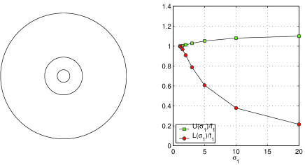
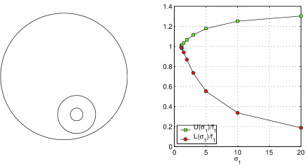
Figure 7: The bounds with increasing $\sigma_{1}$ when the inclusion is an annulus. We take Neumann and Dirichlet data of the special forms. The second and third columns are graphs of the same data; the third column is with a log-scale for the $\sigma_{1}$-axis.

Example 7.2

(variation of $f_{1}$). We compute the bounds for various volume fractions. Figure 8 shows the numerical results. It clearly shows that the lower bound works better for higher volume fractions.

Figure 8: $\sigma_{1}=5$. The bounds changing the volume fraction. We take Neumann and Dirichlet data with the special forms.

Example 7.3

(variation of distance from $\partial\Omega$). We compute the lower and upper bounds changing the distance between the inclusion and $\partial\Omega$. Figure 9 shows the numerical results when $\sigma_{1}=2$. It shows that the further the inclusion is from $\partial\Omega$, the better bounds are.

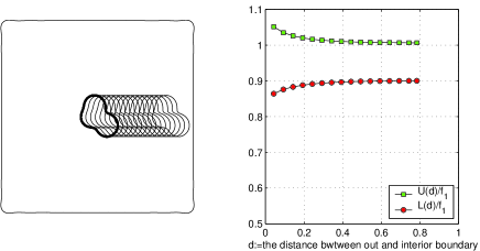
Figure 9: $\sigma_{1}=2$ and $f_{1}=0.0262$. The bounds changing the distance between the inclusion and $\partial\Omega$. We take Neumann and Dirichlet data of the special forms.

Example 7.4

(boundary data). In the example we compute the bounds using other boundary data. We use as Neumann data for the lower bound $q_{1}=-n_{1}-n_{1}n_{2}$ and $q_{2}=-n_{2}-n_{1}n_{2}$, and as Dirichlet data for the upper bound $V_{1}=-x-xy$ and $V_{2}=-y-xy$. Figure 10 shows that the special boundary data work much better.

Figure 10: The bounds changing $\sigma_{1}$ in case that we take Neumann data $g_{1}=-\nu_{1}-\nu_{1}\nu_{2}$ and $g_{2}=-\nu_{2}-\nu_{1}\nu_{2}$. Also we take Dirichlet data $V_{1}=-x-xy$ and $V_{2}=-y-xy$.

Example 7.5

When we use special Neumann data $q_{1}=-n_{1}$ and $q_{2}=-n_{2}$, then a pair of Dirichlet data are measured on $\partial\Omega$. We may use this data to compute the upper bound using the formula (2.67). Likewise, we may use the measured Neumann data corresponding to the Dirichlet data $V_{1}=-x$ and $V_{2}=-y$ to compute the lower bound using the formula (2.48). Figure 11 shows numerical results when the volume fraction varies. In this example it clearly shows that bounds using the measured data are better than those using the given data.

Figure 11: $\sigma_{1}=5$. $L_{N}(f_{1})$ is the lower bound using the Neumann data corresponding to the special Dirichlet data and $U_{D}(f_{1})$ is the upper bound using the Dirichlet data corresponding to the special Neumann data.

8 Construction of E_Ω-inclusions

Following the method outlined in section 23.9 of [23] we look for a simply connected inclusion inside which the field is uniform for some boundary condition assigned on the outer boundary. More precisely, we look for an inclusion $E$ contained in a domain $\Omega$ (bounded or unbounded) such that $-\nabla V$ is uniform inside $E$, where $V$ is the solution to

$$\left\{\begin{array}[]{l}\nabla\cdot\sigma\nabla V=0\quad\mbox{in }\Omega,\\ V=V^{0}\quad\mbox{on }\partial\Omega\end{array}\right.$$ (8.1)

for some boundary data $V^{0}$ with $\sigma=\sigma_{1}\chi(E)+\sigma_{2}\chi(\Omega\setminus E)$ ($\sigma_{1}\neq\sigma_{2}$). We may suppose, without loss of generality, that ${\bf e}=-\nabla V=(-1,0)^{T}$. We also suppose that the coordinates have been positioned and scaled so that $y_{\mbox{max}}=1$ and $y_{\mbox{min}}=-1$, where $y_{\mbox{max}}=\max\{y~{}|~{}(x,y)\in E\mbox{ for some }x\}$ and $y_{\mbox{min}}=\min\{y~{}|~{}(x,y)\in E\mbox{ for some }x\}$. Let $W$ be a harmonic conjugate of $V$ in $\Omega\setminus\overline{E}$ so that $V+iW$ is an analytic function of $z=x+iy$ in $\Omega\setminus\overline{E}$. Then we have

$$V=x,\quad W=\frac{\sigma_{1}}{\sigma_{2}}y,\quad\mbox{on }\partial E.$$ (8.2)

Define new potentials $u$ and $v$ by

$$u+iv=\frac{i(V+iW-z)}{(1-\sigma_{1}/\sigma_{2})}.$$ (8.3)

Then, $u+iv$ is still an analytic function of $z=x+iy$ in $\Omega\setminus\overline{E}$, and on $\partial E$

$$u=\frac{-W+y}{1-\sigma_{1}/\sigma_{2}}=y,\quad v=\frac{V-x}{1-\sigma_{1}/\sigma_{2}}=0.$$ (8.4)

Now assume $u+iv$ is a univalent function of $z=x+iy$ inside $\Omega\setminus\overline{E}$, and consider $x+iy$ as an analytic function of $u+iv$ (hodograph transformation). Because of (8.4), the image of $\partial E$ by $u+iv$ is the slit $S=[y_{\mbox{min}},y_{\mbox{max}}]=[-1,1]$ on the $u$-axis, and $y=u$ on $S$.

The problem is now to construct a function $z=x+iy=f(u+iv)$ such that

• $f$ is analytic and univalent in $U\setminus S$ for some neighborhood $U$ of $S$,

• $\mathop{\rm Im}\nolimits f=u$ on $S$,

• $\mathop{\rm Re}\nolimits f|_{+}-\mathop{\rm Re}\nolimits f|_{-}>0$ on $S$ except at $\pm 1$ where it is $0$.

Here $|_{+}$ and $|_{-}$ indicate the limit from above and below $S$, respectively.

One can see that the conditions (i), (ii), and (iii) guarantee that $f$ maps $U\setminus S$ onto $\Omega\setminus\overline{E}$ for a simply connected domain $E$ and $\Omega$ a domain containing $\overline{E}$. In fact, (ii) and (iii) imply that $f$ maps $S$ onto $\partial E$ and the orientation is preserved. Since $f$ is conformal, it maps $U\setminus S$ to outside $\overline{E}$.

We have the following lemma for univalence.

Lemma 8.1

Let $\gamma$ be a simple closed curve which consists of two curves $\gamma^{+}$ and $\gamma^{-}$. Let $U$ be an open neighborhood of $S$ and let $B_{1}(\delta)$ and $B_{-1}(\delta)$ be open balls of radius $\delta$ centered at $w=1$ and $w=-1$ respectively. Let $f$ be an analytic function in $U\setminus S$ which maps $U\setminus S$ outside $\gamma$ of the form

$$f(w)=iw+g(w)$$ (8.5)

where $\mathop{\rm Im}\nolimits g=0$ on $S$. Suppose that the mapping $u\mapsto\lim_{v\to 0^{+}}f(u+iv)$ is one-to-one from $S$ onto $\gamma^{+}$, and $u\mapsto\lim_{v\to 0^{+}}f(u-iv)$ is one-to-one from $S$ onto $\gamma^{-}$. If there is $\delta>0$ such that $f$ is univalent in $B_{1}(\delta)\setminus S$ and in $B_{-1}(\delta)\setminus S$, then there is an open neighborhood $U_{0}$ of $S$ such that $f$ is univalent in $U_{0}\setminus S$.

Proof: Let $\varphi(z)=(z+\frac{1}{z})/2$ for $|z|\geq 1$. $\varphi$ maps $|z|>1$ onto $\mathbb{C}\setminus S$ and $|z|=1$ onto $S$. Let $G(z)=g(\varphi(z))$. Since $\mathop{\rm Im}\nolimits G(z)=0$ on $|z|=1$, $G$ can be extended so that it is analytic in $1-\varepsilon<|z|<1+\varepsilon$ for some $\varepsilon>0$. Let $F(z)=f(\varphi(z))$. Then $F$ is analytic in $1-\varepsilon<|z|<1+\varepsilon$ and univalent in the neighborhoods of $z=1$ and $z=-1$. Moreover, $F$ is one-to-one from $|z|=1$ onto $\gamma$. We claim that $F$ is univalent in $1-\varepsilon_{0}<|z|<1+\varepsilon_{0}$ for some $\varepsilon_{0}>0$. In fact, if not, then for each $n$ there are $z_{1,n}$ and $z_{2,n}$ such that $1-\frac{1}{n}<|z_{j,n}|<1+\frac{1}{n}$, $z_{1,n}\neq z_{2,n}$, and $F(z_{1,n})=F(z_{2,n})$. For $j=1,2$, the sequence $z_{j,n}$ has a subsequence which converges to a point on $|z|=1$, say $z_{j}$. Since $F$ is one-to-one on $|z|=1$, $z_{1}=z_{2}$. But this implies that $F^{\prime}(z_{1})=0$, where

$$F^{\prime}(z)=f^{\prime}(\varphi(z))\varphi^{\prime}(z)=[i+g^{\prime}(\varphi(z))](1-z^{-2})/2,$$ (8.6)

and since $g^{\prime}(\varphi(z_{1}))$ is real we conclude that $z_{1}=1$ or $z_{1}=-1$ which is contradiction since $F$ is univalent in the neighborhoods of these points. Thus $F$ is univalent in $1-\varepsilon_{0}<|z|<1+\varepsilon_{0}$ for some $\varepsilon_{0}>0$. This completes the proof.   

We now construct $f$ satisfying (i), (ii), and (iii) using conformal mappings. Let $w=u+iv$ and define

$$g(w)=f(w)-iw$$ (8.7)

so that $\mathop{\rm Im}\nolimits g=0$ on $S$. Let

$$\xi=\frac{1-w}{1+w},$$ (8.8)

which maps $S$ onto the positive real axis. Let $\zeta=\sqrt{\xi}$ with the branch cut along the positive real axis and define

$$F(\zeta)=g\left(\frac{1-\zeta^{2}}{1+\zeta^{2}}\right).$$ (8.9)

Then $\mathop{\rm Im}\nolimits F=0$ on the whole real axis. Thus, by defining $F(\zeta^{*})=F(\zeta)^{*}$, where $*$ denotes the complex conjugate, $F$ can be extended as an analytic function in a tubular neighborhood of the real axis. Moreover, since $g$ is analytic in a neighborhood of $-1$ except the part of the slit and the bilinear transform $\zeta$ maps a neighborhood of $-1$ onto outside a compact set, $F$ must be analytic in $\mathbb{C}\setminus(K\cup K^{*})$ where $K$ is a compact set in the upper half plane and $K^{*}$ is its symmetric part with respect to the real axis, i.e., $K^{*}=\{z^{*}~{}|~{}z\in K\}$. $F$ satisfies

• $F$ is analytic in $\mathbb{C}\setminus(K\cup K^{*})$ for a compact set $K$ in the upper half plane.

• $\mathop{\rm Im}\nolimits F=0$ on the real axis,

• $F(\zeta)-F(-\zeta)>0$ for real positive $\zeta$.

The function $f$ is now given by

$$f(w)=iw+F\left(\sqrt{\frac{1-w}{1+w}}.\right)$$ (8.10)

Note that $y=u$ on the slit and hence $\partial E$ is given by

$$x=F\left(\pm\sqrt{\frac{1-y}{1+y}}\right).$$ (8.11)

In addition to (i)^′, (ii)^′, and (iii)^′, $F$ needs to be univalent inside a suffiently small ball around the origin, and outside a sufficiently large ball. The first condition is satisfied if $F^{\prime}(0)\neq 0$. Since $F$ maps $\infty$ to a point in $\mathbb{C}$, $F$ being analytic and univalent outside a sufficiently large ball has the series expansion

$$F(\zeta)=\sum_{j=0}^{\infty}\frac{\beta_{j}}{\zeta^{j}}$$ (8.12)

as $\zeta\to\infty$, where $\beta_{1}\neq 0$ (and $\beta_{1}$ is real and positive from conditions (ii)^′, and (iii)^′).

We make a record of these conditions:

• The derivative $F^{\prime}(0)$ is non-zero, and $F(\zeta)$ has the asymptotic expansion

  $$F(\zeta)=\beta_{0}+\frac{\beta_{1}}{\zeta}+O(|\zeta|^{-2})\quad\mbox{as }|\zeta|\to\infty,$$ (8.13)

  where $\beta_{1}$ is real and positive.

Good candidates for functions satisfying (i)^′, (ii)^′, and (iv)^′ are rational functions of the form

$$F(\zeta)=\sum_{\alpha=1}^{n}\left[\frac{b_{\alpha}}{\zeta-a_{\alpha}}+\frac{b_{\alpha}^{*}}{\zeta-a_{\alpha}^{*}}\right]+c$$ (8.14)

where the $a_{\alpha}$’s are complex numbers with positive imaginary parts, the $b_{\alpha}$’s are complex numbers, $c$ is a real number, and

$$\sum_{\alpha=1}^{n}\mathop{\rm Re}\nolimits(b_{\alpha})>0,\quad\sum_{\alpha=1}^{n}\mathop{\rm Re}\nolimits(b_{\alpha}/a_{\alpha}^{2})\neq 0.$$ (8.15)

To ensure that (iii)^′ is satisfied we require that the function

$$F(\zeta)-F(-\zeta)=2\zeta\sum_{\alpha=1}^{n}\left[\frac{b_{\alpha}}{\zeta^{2}-a_{\alpha}^{2}}+\frac{b_{\alpha}^{*}}{\zeta^{2}-(a_{\alpha}^{*})^{2}}\right]$$ (8.16)

has no real roots aside from $\zeta=0$. (The sign of the inequality in (iii)^′ is guaranteed by the positivity of $\beta_{1}$.)

Let us now characterize those rational functions $F$ which yield ellipses as E_Ω-inclusions. Because $y=u$ on the slit $[-1,1]$, the ellipse takes the shape like the first figure in Figure 14 (after translation). Let the ellipse be given by $x^{2}+\alpha y^{2}+\beta xy=c$ with $4\alpha>\beta^{2}$. Solving for $x$ we get

$$x=\frac{-\beta y\pm\sqrt{\beta^{2}y^{2}-4(\alpha y^{2}-c)}}{2}.$$ (8.17)

Since the discriminant vanishes at $y=\pm 1$, we have $c=4\alpha-\beta^{2}$, and hence

$$x=\frac{-\beta}{2}y\pm\frac{(1+y)}{2}\sqrt{(4\alpha-\beta^{2})\frac{1-y}{1+y}}.$$ (8.18)

Letting $\zeta=\sqrt{\frac{1-y}{1+y}}$, we have

$$x=\frac{\pm\zeta\sqrt{4\alpha-\beta^{2}}-\beta}{\zeta^{2}+1}+\frac{\beta}{2}=F(\zeta)$$ (8.19)

for real $\zeta$. It means that ellipses are obtained by $F$’s of the form

$$F(\zeta)=\frac{b}{\zeta-a}+\frac{b^{*}}{\zeta-a^{*}}+c$$ (8.20)

with $a=i$ and $b$ with positive real part.

Example. In this example, we construct some E_Ω-inclusions other than ellipses. We use $F$ in the form (8.20) with $c=0$ (it amounts to translating the figure). Then in $\zeta$-coordinates $f$ is given by

$$f(\zeta)=\frac{2i}{\zeta^{2}+1}+\frac{b}{\zeta-a}+\frac{b^{*}}{\zeta-a^{*}}.$$ (8.21)

where both (8.15) and the absence of real non-zero roots of (8.16) will be ensured if we choose $b$ and $-b/a^{2}$ with positive real parts.

We will plot the image of a vicinity of the real axis in the upper half plane under the map $f$. To avoid computational difficulty in dealing with an infinite space, we use a bilinear transform

$$\zeta=\frac{1-iw}{w-i},$$ (8.22)

which maps the unit disk onto the upper half plane. Then we plot

$$f(w)=\frac{2i}{\zeta(w)^{2}+1}+\frac{b}{\zeta(w)-a}+\frac{b^{*}}{\zeta(w)-a^{*}}$$ (8.23)

for $w=re^{i\theta}$ with $1-\varepsilon\leq r\leq 1$. From the expansions for $F(\zeta)$ in powers of $\zeta$ and $1/\zeta$ we see that near the bottom and top of the inclusion the boundary is given by

$$x\approx\mathop{\rm Re}\nolimits(b)\sqrt{2(1+y)}+O(1+y),\quad\quad x\approx-2\mathop{\rm Re}\nolimits(b/a)-\mathop{\rm Re}\nolimits(b/a^{2})\sqrt{2(1-y)}+O(1-y).$$ (8.24)

Thus the bottom and top are positioned at $x=0$ and $x=-2\mathop{\rm Re}\nolimits(b/a)$ and the curvature of the boundary there is determined by $\mathop{\rm Re}\nolimits(b)$ and $-\mathop{\rm Re}\nolimits(b/a^{2})$ respectively.

Figure 13 shows various shapes of $\partial\Omega$, which are the image of $|z|=r<1$ under $f$, and the boundary of E_Ω-inclusion, which is the image of $|z|=1$. Figure 12, 14, 15, 16, 17, and 18 show various shapes of E_Ω-inclusions when we vary the complex parameters $a$, $b$, and $b/a^{2}$.

We emphasize that with these values of $a$ and $b$, the univalence of $f$ is guaranteed by Lemma 8.1.

Figure 12: Various shapes of E_Ω-inclusions when varying Re $a$ with Im $a=1$ and $b=1$.

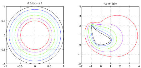
Figure 13: With $a=0.8+i$ and $b=1$, the inner most curve (the image of $|z|=1$) is the boundary of the E_Ω-inclusion (the rightmost inclusion in Fig. 12). The others are images of $|z|=0.9,\ 0,8,\ 0,7,\ 0,6,\ 0,5$. These, or any simple closed curve enclosed by them, can be regarded as boundaries of $\Omega$.

Figure 14: Various shapes of E_Ω-inclusions when varying Im $a$ with Re $a=0$ and $b=1+i$.

Figure 15: Various shapes of E_Ω-inclusions when varying Re $b$ with Im $b=1$ and $a=1.3i$.

Figure 16: Various shapes of E_Ω-inclusions when varying Im $b$ with Re $b=1$ and $a=1.3i$.

Figure 17: Various shapes of E_Ω-inclusions when varying Im $b$ with Re $b=0.1$ and $b/a^{2}=-10+2i$.

Figure 18: Various shapes of E_Ω-inclusions when varying Im $b/a^{2}$ with $b=0.1+2i$ and Re $b/a^{2}=-10$.

References

- [1] G. Alessandrini and E. Rosset, The inverse conductivity problem with one measurement: bounds on the size of the unknown object, SIAM J. Appl. Math., 58 (1998), 1060–1071.
- [2] G. Alessandrini, E. Rosset, and J.K. Seo, Optimal size estimates for the inverse conductivity problem with one measurement, Proc. Amer. Math. Soc., 128 (2000), 53–64.
- [3] G. Allaire, Shape Optimization by the Homogenization Method, Applied Mathematical Sciences, Vol. 146 , Springer-Verlag, 2002.
- [4] H. Ammari and H. Kang, Reconstruction of Small Inhomogeneities from Boundary Measurements, Lecture Notes in Mathematics, Vol. 1846, Springer-Verlag, Berlin, 2004.
- [5] H. Ammari and H. Kang, Polarization and Moment Tensors: with Applications to Inverse Problems and Effective Medium Theory, Applied Mathematical Sciences, Vol. 162, Springer-Verlag, New York, 2007.
- [6] Y. Capdeboscq and M.S. Vogelius, Optimal asymptotic estimates for the volume of internal inhomogeneities in terms of multiple boundary measurements, Math. Modelling Num. Anal., 37 (2003), 227–240.
- [7] Y. Capdeboscq and M.S. Vogelius, A review of some recent work on impedance imaging for inhomogeneities of low volume fraction, Proceedings of the Pan-American Advanced Studies Institute on PDEs, Inverse Problems and Nonlinear Analysis, January 2003, 69–87, Contemp. Math., 362, Amer. Math. Soc., Providence, RI, 2005.
- [8] G.P. Cherepanov, Inverse problems of the plane theory of elasticity, PMM Vol. 38 (1974), 963-979.
- [9] A.V. Cherkaev, Variational Methods for Structural Optimization , Applied Mathematical Sciences, Vol. 140 , Springer-Verlag, 2000.
- [10] J.D. Eshelby, Elastic inclusions and inhomogeneities. In Progress in Solid Mechanics, ed. by I.N. Sneddon and R. Hill, Vol. II (1961) 87–140, North-Holland, Amsterdam.
- [11] Y. Grabovsky, Bounds and extremal microstructures for two-component composites: A unified treatment based on the translation method, Proc. Roy. Soc. Lond. A, 452 (1996), 919–944.
- [12] H. Kang, Conjectures of Polya-Szego and Eshelby, and the Newtonian Potential Problem; A Review, Mechanics of Materials, 41 (2009), 405-410.
- [13] H. Kang, E. Kim, and G.W. Milton, Inclusion pairs satisfying Eshelby’s uniformity property, SIAM J. Appl. Math. 69 (2008), 577-595.
- [14] H. Kang and G.W. Milton, On Conjectures of Polya-Szego and Eshelby, in lnverse Problems, Multi-scale Analysis and Effective Medium Theory (H. Kang and H. Ammari Eds.), Contemporary Math. 408 (2006), 75-80.
- [15] H. Kang and G.W. Milton, Solutions to the Pólya-Szegö Conjecture and the Weak Eshelby Conjecture, Arch. Rational Mech. Anal. 188 (2008), 93-116.
- [16] H. Kang, J.K. Seo, and D. Sheen, The inverse conductivity problem with one measurement: stability and estimation of size, SIAM J. Math. Anal., 28 (1997), 1389–1405.
- [17] J.G. Berryman and R.V. Kohn, Variational constraints for electrical-impedance tomography, Phys. Rev. Lett. 65 (1990), 325–328.
- [18] R. Lipton, Inequalities for electric and elastic polarization tensors with applications to random composites, J. Mech. Phys. Solids 41 (1993), 809–833.
- [19] L.P. Liu, Solutions to the Eshelby conjectures, Proc. R. Soc. A. 464 (2008), 573-594.
- [20] L.P. Liu, R. James, and P. Leo, New extremal inclusions and their applications to two-phase composites, preprint.
- [21] K.A. Lurie and A.V. Cherkaev, Accurate estimates of the conductivity of mixtures formed of two materials in a given proportion (two-dimensional problem), Doklady Akademii Nauk SSSR 264 (1982) 1128–1130. English translation in Soviet Phys. Dokl. 27 (1982), 461–462.
- [22] K.A. Lurie and A.V. Cherkaev, Exact estimates of conductivity of composites formed by two isotropically conducting media taken in prescribed proportion, Proc. Royal Soc. Edinburgh A, 99 (1984), 71–87.
- [23] G.W. Milton, The Theory of Composites, Cambridge Monographs on Applied and Computational Mathematics, Cambridge University Press, 2002.
- [24] G.W. Milton, Transport properties of arrays of intersecting cylinders, Appl. Phys. 25 (1981), 23–30.
- [25] G.W. Milton, Universal bounds on the electrical and elastic response of two-phase bodies and their application in bounding the volume fraction from boundary measurements. In preparation.
- [26] F. Murat and L. Tartar, Calcul des variations et homogénísation, in Les méthodes de l’homogénéisation: théorie et applications en physique, pp. 319–369 Eyrolles, 1985. English translation in Topics in the Mathematical Modelling of Composite Materials (A. Cherkaev and R. Kohn Eds), Progress in Nonlinear Differential Equations and Their Applications 31 (1997) 139–173, Birkhäuser.
- [27] G.P. Sendeckyj, Elastic inclusion problems in plane elastostatics, Int. J. Solids Structures 6 (1970), 1535–1543.
- [28] L. Tartar, Estimation de coefficients homogénéisés, in Computing Methods in Applied Sciences and Engineering: Third International Symposium, Versailles, France, December 5–9, 1977 (R. Glowinski and J.-L. Lions Eds.), Lecture Notes in Mathematics 704 (1979) 364–373, Springer-Verlag. English translation in Topics in the Mathematical Modelling of Composite Materials (A. Cherkaev and R. Kohn Eds), Progress in Nonlinear Differential Equations and Their Applications 31 (1997) 9–20, Birkhäuser.
- [29] L. Tartar, Estimations fines des coefficients homogénéisés, in Ennio de Giorgi Colloquium: Papers Presented at a Colloquium Held at the H. Poincaré Institute in November 1983 (P. Krée Ed.) Pitman Research Notes in Mathematics 125 (1985) 168–187, Pitman.
- [30] L. Tartar, The General Theory of Homogenization: A Personalized Introduction, Lecture Notes of the Unione Matematica Italiana, Springer-Verlag, 2009.