Topological Transitions for Lattice Bosons in a Magnetic Field

Abstract

The Hall response provides an important characterization of strongly correlated phases of matter. We study the Hall conductivity of interacting bosons on a lattice subjected to a magnetic field. We show that for any density or interaction strength, the Hall conductivity is characterized by a single integer. We find that the phase diagram is intersected by topological transitions between different integer values. These transitions lead to surprising effects, including sign reversal of the Hall conductivity and extensive regions in the phase diagram where it acquires a negative sign. This implies that flux flow is reversed in these regions - vortices there flow upstream. Our finding have immediate applications to a wide range of phenomena in condensed matter physics, which are effectively described in terms of lattice bosons.

The Hall response is a key theoretical and experimental tool for characterizing emergent charge carriers Ziman in strongly correlated systems, ranging from high temperature superconductors Hagen90 ; LeBoeuf07 ; LeBoeuf11 to the quantum Hall effect Wen95 . In this paper, we study the Hall conductivity of strongly correlated bosons on a lattice. We find that the entire phase diagram of such systems can be characterized using a single integer $p$, and inevitably contains topological transitions between different $p$ - values. These observations allow us to calculate the Hall conductivity throughout the whole phase diagram, and we show that they lead to surprising consequences, such as sign reversals of the Hall conductivity. The model we study describes a wide range of systems in condensed matter physics, to which our results have immediate implications. Examples are cold atoms on optical lattices Jaksch98 ; Jaksch05 , Josephson junction arrays Fazio01 , granular superconductors Simanek79 ; Doniach81 , and perhaps even high temperature superconductors such as the underdoped cuprates Uemura89 ; Micnas95 ; Mihlin09 .

In the absence of disorder and at weak magnetic fields the Hall conductivity of bosonic systems is dominated by the flow of superfluid vortices. For a continuum (Galilean invariant) superfluid, vortex flow gives a Hall conductivity which is proportional to the ratio of the particle density and the applied magnetic field. We find that on the lattice, vortex dynamics is strongly modified. As a result the Hall conductivity is characterized, in addition to the particle density, by the integer $p$. We show how emergent particle-hole symmetry points in the ground-state phase diagram necessarily lead to a non-trivial behavior of this integer and we discuss the topological transitions between different $p$-sectors. As we shall show, these transitions are attributed to degeneracies in the many body spectrum, which serve as sources for the Berry curvature.

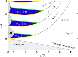
Figure 1: Topological transitions in the Bose-Hubbard phase diagram. The Galilean invariant regime denotes the region where $\sigma_{xy}$ is proportional to the particle density $n_{b}$ divided by the magnetic field strength $B$. Mott insulator lobes are indicated in gray. The yellow and green lines exhibit an emergent particle hole symmetry, where $\sigma_{xy}=0$. They are divided into two types: (i) Lines emanating from the tip of the Mott lobe at integer boson filling where $\sigma_{xy}$ has a smooth zero crossing (green). (ii) Transition lines (yellow), through which $B\sigma_{xy}$ exhibits integer jumps. The latter continue into the phase diagram, with $\sigma_{xy}>0$, as indicated by the dashed lines. The blue region corresponds to regions where the Hall conductivity is negative.

Specifically, we focus on the conventional Bose-Hubbard model Fisher89 in two dimensions. We restrict our study to a dissipation-less system, at zero temperature and without disorder. Within the phase diagram of this model we find large parameter regions corresponding to a negative Hall conductivity, $\sigma_{xy}<0$, and reversed vortex motion where vortices flow upstream, cf. Fig 1. We discuss methods to directly test these results in cold atom systems where the neutral atoms are subjected to synthetic magnetic fields introduced through rotation or phase imprinting Lin09 ; Cooper11 .

I Hall conductivity and vortex motion

We begin by giving a description of vortex dynamics in bosonic systems. A vortex moving with respect to a current experiences a force arising from the interaction of the velocity field of the vortex with the one of external current. This hydrodynamical force is called the Magnus force, and it acts perpendicularly to the current, as depicted in Fig. 2(a). Similarly, a superfluid vortex (of unit vorticity) in two dimensions experiences a force

$${\bf F}_{\scriptscriptstyle\rm M}=-2\pi\hbar n_{s}{\bf v}_{s}\times\hat{\bf e}_{z}.$$ (1)

where $n_{s}$ is the number density of superfluid bosons, and ${\tenmib v}_{s}$ is their velocity. The unit vector $\hat{\bf e}_{z}$ is a normal to the plane.

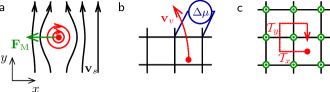
Figure 2: Forces acting on a vortex. (a) The classical Magnus force due to the interaction of the velocity field of the vortex and the external flow ${\bf v}_{s}$ acts perpendicular to ${\bf v}_{s}$. (b) Vortex motion leads to a change in the momentum of the system due to its phase singularity, which is perpendicular to its velocity ${\bf v}_{v}$. (c) Moving a vortex around a lattice site yields a Berry phase of $2\pi\alpha=2\pi(n_{b}+p)$.

The force ${\bf F}_{\scriptscriptstyle\rm M}$ in Eq. (1) arises from the dynamical phase (time integral of the energy) in a Lagrangian describing the superfluid. Such a Lagrangian necessarily contains a term corresponding to the Berry phase picked up by the vortex motion. The Berry phase acquired by a vortex moving around a loop of area $S$ is given by $2\pi\alpha S$, where $\alpha$ is a proportionality factor which depends on the microscopic details of the Hamiltonian. Therefore, an equation of motion for the vortex leading to dissipation-less flow is linear in the vortex velocity and given by Fisher91

$${\bf F}_{\scriptscriptstyle\rm M}+2\pi\hbar\alpha\,{\bf v}_{v}\times\hat{\bf e}_{z}=0.$$ (2)

Equation (2) can also be understood from the perspective of momentum balance. A moving vortex imprints a phase discontinuity on the superfluid wave function. The Josephson relation $\Delta\mu=\hbar\partial_{t}\Delta\varphi$ connects the resulting chemical potential to the time derivative of the relative phase difference, cf. Fig. 2(b). The chemical potential drop will be balanced by a flow of particles, which results in momentum transfer from the particles to the moving vortex, perpendicular to the vortex velocity ${\bf v}_{v}$ and proportional to its magnitude. The proportionality factor $\alpha$ relates the change in the system’s momentum to the vortex velocity.

The Hall conductivity can be related to the drift velocity of a vortex. From (1) and (2) we get

$${\bf v}_{v}={\textstyle{n_{s}\over\alpha}}\bf{v}_{s}.$$ (3)

In a system with a low density of vortices we can neglect the effects of vortex-vortex interactions. Considering strictly dissipation-less flow, we obtain from the Josephson relation a semi-classical expression for the Hall conductivity

$$\sigma_{xy}={\textstyle{qn_{s}v_{s}\over\Delta\mu}}={\textstyle{q^{2}n_{s}v_{s}\over 2\pi\hbar n_{v}v_{v}}}={\textstyle{q^{2}\over h}}{\textstyle{\alpha\over n_{v}}}.$$ (4)

where $n_{v}$ is the density of vortices and $q$ the boson charge.

In systems with Galilean invariance, in a reference frame moving at the vortex velocity, there should be no forces acting on the vortex. This requires ${\tenmib v}_{v}={\tenmib v}_{s}$ and therefore sets $\alpha=n_{s}$ Haldane85 ; Ao93 . This relation is modified in the presence of a lattice, as we discuss now.

We consider the standard model for interacting bosons on a lattice Fisher89

$${\cal H}= - t\sum_{\langle{\tenmib r},{\tenmib r}^{\prime}\rangle}\Bigl{[}b_{{\tenmib r}}^{{\dagger}}b_{{\tenmib r}^{\prime}}^{\phantom{{\dagger}}}e^{iA_{{\tenmib r}{\tenmib r}^{\prime}}}+b_{{\tenmib r}}^{{\dagger}}b_{{\tenmib r}^{\prime}}^{\phantom{{\dagger}}}e^{-iA_{{\tenmib r}{\tenmib r}^{\prime}}}\Bigr{]}$$ (5)

$$+ {\textstyle{U\over 2}}\sum_{{\tenmib r}}b_{{\tenmib r}}^{{\dagger}}b_{{\tenmib r}}^{\phantom{{\dagger}}}(b_{{\tenmib r}}^{{\dagger}}b_{{\tenmib r}}^{\phantom{{\dagger}}}-1)-\mu\sum_{{\tenmib r}}b_{{\tenmib r}}^{{\dagger}}b_{{\tenmib r}}^{\phantom{{\dagger}}},$$

where $b_{{\tenmib r}}^{{\dagger}}$ creates a boson on site ${\tenmib r}$, $t$ is the hopping amplitude, $U$ the on-site repulsion; $A_{{\tenmib r}{\tenmib r}^{\prime}}=q\int_{{\tenmib r}}^{{\tenmib r}^{\prime}}\bf{A}\cdot{\bf dx}$ is the phase factor due to applied gauge field ${\bf A}$. We work in units where $\hbar=c=1$, and likewise we set the lattice constant $a=1$.

We first note that vortices live on the center of the plaquettes of the lattice. We explicitly construct operators $\mathcal{T}_{x}$ and ${\cal T}_{y}$ which translate a vortex by one lattice constant in the $x$ and $y$ directions. We show that they obey the commutation relation (see supplementary materials for a full derivation)

$$\mathcal{T}_{x}\mathcal{T}_{y}=\mathcal{T}_{y}\mathcal{T}_{x}e^{2\pi i\hat{N_{b}}/N}.$$ (6)

Here, $\hat{N}_{b}$ is the total boson number operator, and $N$ is the number of sites. We denote the particle filling by $n_{b}=N_{b}/N$. From Eq. (6), we see that the Berry phase acquired by moving a vortex around a dual lattice plaquette is

$$2\pi\alpha=2\pi(n_{b}+p)\qquad\mbox{with}\qquad p\in\mathbb{Z}.$$ (7)

The integer $p$ arises from the $2\pi$ ambiguity in Eq. (6).

Equation (7) can also be understood in terms of momentum balance Oshikawa00 . Following Paramekanti and Vishwanath Paramekanti04 , we note that Eq. (6) implies that when a vortex is transported by $\Delta y$ sites along $\hat{\bf e}_{y}$, the momentum of the system changes by $\Delta P_{x}=2\pi n_{b}\Delta y$. At the same time we can integrate Eq. (2) to obtain $\Delta P_{x}=2\pi\alpha\Delta y$. Combining the two results and taking into account that momentum is only conserved up to a reciprocal lattice vector $2\pi p$ leads us to Eq. (7).

The above results, together Eq. (4), imply a similar relation for the Hall conductivity,

$$\sigma_{xy}\,n_{v}={\textstyle{q^{2}\over h}}\left(n_{b}+p\right)\qquad\mbox{with}\qquad p\in\mathbb{Z}.$$ (8)

While Eqs. (4) and (8) are a semi-classical derivation of the Hall conductivity, in Sec. IV we derive an exact relation between $\alpha$ and the Hall conductivity for a system containing one vortex,

$$\sigma_{xy}={\textstyle{q^{2}\over h}}N\alpha={\textstyle{q^{2}\over h}}N(n_{b}+p)\qquad\mbox{with}\qquad p\in\mathbb{Z}.$$ (9)

In the remainder of this paper we investigate the relations (7–9) throughout the phase diagram of the Bose-Hubbard model. In Sec. II we study these relations in the Gross-Pitaevskii and Mott transition limits. In Sections III, IV we study the transition between different $p$-sectors in the hard core boson limit. We complete the phase diagram using numerical calculations in Sec. V.

II Low-energy limits

We start by discussing low energy limits of Eq. (5) where a diverging length-scale enables the derivation of a continuum low-energy theory. In these limits $\alpha$ and $\sigma_{xy}$ can be deduced directly. We review the derivation of the low-energy theories for weak ($U\ll t$) and strong ($U\gg t$) interactions. In both cases we start by rewriting (5) as a coherent state path integral with the following action for the complex valued field $\psi_{i}$

$$S=\int\!\!d\tau\,\Bigg{\{}\sum_{i}\psi_{i}^{*}(\partial_{\tau}-\mu)\psi_{i}-t\sum_{\langle i,j\rangle}(\psi_{i}^{*}\psi_{j}e^{-i\varphi_{ij}}+{\rm c.c.})\\ +{\textstyle{U\over 2}}\sum_{i}|\psi_{i}|^{2}(|\psi_{i}|^{2}-1)\Bigg{\}}.$$ (10)

The Gross-Pitaevskii limit – In the weakly interacting limit, the Gross-Pitaevskii healing length $\xi_{\scriptscriptstyle\rm GPE}=a\sqrt{t/Un_{b}}$ is much larger than the lattice spacing $a$. This enables a straight-forward gradient expansion of (10). To lowest order in gradients we obtain the continuum action

$$S=\int\!\!d\tau d{\bf x}\,\Big{\{}\psi^{*}\partial_{\tau}\psi+a^{2}t|(\nabla-iq{\bf A})\psi|^{2}+\dots\Big{\}}.$$ (11)

Using the above expression we can now derive the coefficient $\alpha$ in the Gross-Pitaevskii limit. When written in terms of $\psi=\sqrt{n_{b}}\exp(i\vartheta)$, the term $\psi^{*}\partial_{\tau}\psi$ in Eq. (11) leads to a purely imaginary ${\mathcal{L}}_{\tau}=2\pi imn_{b}$, where $m$ is a field that counts the winding of the phase $\vartheta$ Fisher91 . Consider the action of a field configuration associated with taking a vortex around a closed loop of area $S$. A little reflection shows that the regions outside the loop do not change the value of $m$ while those inside contribute unity per particle. Hence, $\mathcal{L}_{\tau}$ gives rise to a Berry phase of $2\pi in_{b}S$ Haldane85 . This observations fixes

$$\alpha=n_{b}.$$ (12)

Around the Mott insulator – At strong interactions and integer filling, $n_{b}\in{\mathbb{N}}$, the Hamiltonian (5) stabilizes a localized Mott insulating phase with vanishing superfluid fraction $\bar{\psi}_{i}\!\equiv\!\langle\psi_{i}\rangle\!=0$ Fisher89 . In the insulating phase all sites are occupied by exactly $n_{b}$ bosons. Both the addition or removal of a particle is protected by a finite gap. This gap closes at the boundary of the Mott lobes in the phase diagram of Fig. 1, whereby at the lower (upper) boundary of the Mott lobe the hole (particle) gap vanishes. Hence, the tip of the Mott lobe represents a multi-critical point where the particle and hole gap close simultaneously Capogrosso-Sansone07 . In the following we focus on this multi-critical point.

When both the particle and hole gap vanish, an enhanced symmetry in the low energy sector emerges. Instead of going through the standard procedure of deriving the low-energy theory from microscopic considerations Oosten01 ; Polkovnikov05 we motivate the effective action via its symmetry properties. We expect the following particle-hole symmetry (PHS) to hold $\bar{\psi}\rightarrow\bar{\psi}^{*}$ and ${\bf A}\rightarrow-{\bf A}$ Dorsey92 . To leading order in powers of $\bar{\psi}$ we find

$$S=\int\!\!d\tau d{\bf x}\,\Big{\{}{\textstyle{1\over 8tn_{b}}}|\partial_{\tau}\bar{\psi}|^{2}+a^{2}tn_{b}|(\nabla-iq{\bf A})\bar{\psi}|^{2}+\dots\Big{\}}.$$ (13)

The gradient expansion leading to an effective continuum theory is controlled by the diverging correlation length close to the second order phase transition into the Mott insulating state.

A direct consequence of PHS in the continuum theory (13) is $\sigma_{xy}({\bf A})=\sigma_{xy}(-{\bf A})$. Together with the Onsager relation $\sigma_{xy}({\bf A})=-\sigma_{xy}(-{\bf A})$ we obtain $\sigma_{xy}=0$. This result can also be understood in terms of vortex motion. As opposed to the Gross-Pitaevskii action, the continuum theory (13) is real. Hence it does not give rise to any Berry phase when a vortex is moved around a closed loop and we conclude

$$\alpha=0.$$ (14)

Starting from the PHS points, we expect to find lines with $\alpha=0$ in the $\mu/U$–$t/U$ phase diagram of the Bose Hubbard model. From Eq. (7) on the other hand, we know that at a fixed density, $\alpha$ can only change by an integer. This leads to the conclusion that the lines with $\alpha=0$ are bound to lines of integer fillings in the phase diagram, c.f. Fig. 1.

III Hard core bosons limit

We now consider the limit $t/U\to 0$ and $\mu/U\to m$, where $m$ is an integer. In Fig. 1, these limits lie in-between two Mott lobes. The two states with $m$ and $m+1$ bosons per site are degenerate single-site states of Hamiltonian (5). States with different fillings are separated by a gap of order $U$, and do not appear in the low energy theory.

We use a Schrieffer-Wolf transformation macdonald88 to project the Hamiltonian (5) onto the subspace with only $m$ and $m+1$ bosons per site. The resulting Hamiltonian corresponds to hard-core bosons (HCB) and can be written using spin-$1\over 2$ operators; $S^{z}_{i}+\mbox{$1\over 2$}$ is the onsite number operator, and $S^{+}_{i}$ ($S^{-}_{i}$) raises (lowers) the occupation from $m$ to $m+1$ (and vice versa). At zeroth order in $t/U$, the HCB Hamiltonian is given by

$${\cal H}_{\scriptscriptstyle\rm HC}^{(0)}=-(m+1)t\sum_{\langle{\tenmib r},{\tenmib r}^{\prime}\rangle}\left(e^{iA_{{\tenmib r}{\tenmib r}^{\prime}}}S^{+}_{\tenmib r}S^{-}_{{\tenmib r}^{\prime}}+{\rm h.c.}\right)-\mu\sum_{{\tenmib r}}S^{z}_{{\tenmib r}}.$$ (15)

The HCB Hamiltonian (15) has an emergent charge conjugation symmetry. One defines the unitary transformation

$$C\equiv\exp\Big{(}i\pi\sum_{\tenmib r}S^{x}_{\tenmib r}\Big{)}.$$ (16)

$C$ transforms particles into holes, i.e., $C^{\dagger}S^{z}_{\tenmib r}C=-S^{z}_{\tenmib r}$, and

$$C^{\dagger}\,{\cal H}^{(0)}_{\scriptscriptstyle\rm HC}\big{(}q{\tenmib A},\mu\big{)}\,C={\cal H}^{(0)}_{\scriptscriptstyle\rm HC}\big{(}-q{\tenmib A},-\mu\big{)}.$$ (17)

At half filling for the hard core bosons, the Hamiltonian (15) is independent of $\mu$ and hence Eq. (17) implies invariance under ${\bf A}\to-{\bf A}$. Hence, the Onsager relation $\sigma_{xy}({\bf A})=-\sigma_{xy}(-{\bf A})$ implies that for half integer fillings ($n_{b}=\mbox{$1\over 2$}+m$)

$$\sigma_{xy}=\alpha=0.$$ (18)

Note that the situation at the HCB limits and at the tip of the Mott lobes are qualitatively different. The Hall conductivity at the tip of the Mott lobe vanishes due to a zero-crossing of $\alpha$ when $p=-n_{b}$. In the HCB limit, the integer $p$ jumps exactly at $n_{b}=m+\mbox{$1\over 2$}$. In other words: in the first case it reflects a particle hole-symmetry between $n_{b}-1$ and $n_{b}+1$ while in the latter the symmetry connects $n_{b}-1$ and $n_{b}$ at $n_{b}=m+\mbox{$1\over 2$}$. The symmetry at the HCB limits has a remarkable consequence for $\sigma_{xy}$ in the full phase diagram of the model, as we shall now show.

IV Away from the hard core boson limit

We now consider the effect of a finite but small value of $t/U$. Second order processes in which a virtual excitation with an on-site occupation of $m-1$ or $m+2$ bosons are created lead to corrections to the Hamiltonian (15) of order $t^{2}/U$. Taking into account all the different processes we obtain up to irrelevant re-normalizations of the parameters in ${\cal H}_{\scriptscriptstyle\rm HC}$

$${\cal H}_{\scriptscriptstyle\rm HC}^{(1)}\!=\!{\cal H}^{(0)}_{\scriptscriptstyle\rm HC}-\epsilon_{m}\!\!\!\sum_{\langle\langle{\tenmib r},{\tenmib r}^{\prime};{\tenmib r}^{\prime\prime}\rangle\rangle}\!\!\!\left(e^{iA_{{\tenmib r}{\tenmib r}^{\prime}}}S_{{\tenmib r}}^{+}S_{{\tenmib r}^{\prime}}^{-}(S^{z}_{{\tenmib r}^{\prime\prime}}+\mbox{$1\over 2$})+{\rm h.c.}\right),$$ (19)

where $\langle\langle{\tenmib r},{\tenmib r}^{\prime};{\tenmib r}^{\prime\prime}\rangle\rangle$ denote sites ${\tenmib r}$ and ${\tenmib r}^{\prime}$ which are nearest neighbors of site ${\tenmib r}^{\prime\prime}$, and $\epsilon_{m}=(m+1)(m+2)t^{2}/U$.

The new terms in Eq. (19) break the charge conjugation symmetry, and therefore the Hall conductivity at exactly half integer filling does not vanish; below we calculate it in the limit of small $t/U$.

We consider the model Eq. (19) on a torus of size $N=L_{x}L_{y}$, with $N$ even. The gauge field ${\bf A}$ describes a uniform flux penetrating the surface of the torus. We take the total flux to be one flux quantum, which induces one vortex into the system. An important gauge invariant quantity described by the gauge field are the two Wilson line functions Lindner10

$$\Phi_{x}(y)=\oint dxA_{x},\qquad\Phi_{y}(x)=\oint dyA_{y}.$$ (20)

We define $\Theta_{x}=\Phi_{x}(y=0)$ and $\Theta_{y}=\Phi_{y}(x=0)$. Changing the values of $\Theta_{x}$ and $\Theta_{y}$ corresponds to threading Aharonov-Bohm (AB) fluxes through the two holes of the torus Lindner10 .

The Hall conductivity at zero temperature, for a general many-body Hamiltonian can be calculated by integrating the Berry curvature Avron85

$$\sigma_{xy}={q^{2}\over h}{1\over 2\pi}\int\limits_{0}^{2\pi}\!\!d\Theta^{\vphantom{*}}_{x}\!\!\int\limits_{0}^{2\pi}\!\!d\Theta^{\vphantom{*}}_{y}\>{\cal F}.$$ (21)

${\cal F}$ is given by

$${\cal F}=\epsilon^{\mu\nu}\partial_{\Theta_{\mu}}A_{\nu},\qquad{\cal A}_{\nu}=i\left\langle{\Psi_{0}(\boldsymbol{\Theta})}\bigg{|}{\partial\Psi_{0}(\boldsymbol{\Theta})\over\partial\Theta^{\vphantom{*}}_{\nu}}\right\rangle.$$ (22)

Here $\Psi_{0}(\boldsymbol{\Theta})$ is the many-body ground state wave function which depends on the Aharonov-Bohm fluxes through the holes of the torus.

Remarkably, the Hall conductivity in the presence of one vortex can be calculated analytically at half filling. The key ingredients are degeneracies in the spectrum that occur for $t/U=0$ Lindner09 ; Lindner10 and serve as point (monopole) sources for the Berry curvature ${\cal F}$ Simon83 .

To understand the degeneracies, we consider an effective Hamiltonian for the vortex hopping between dual lattice sites. As shown in Ref. Lindner09 ; Lindner10 , this is given by

$${\cal H}_{\textsf{V}}=-t^{\vphantom{*}}_{\textsf{V}}\sum_{\langle{\tenmib R},{\tenmib R}^{\prime}\rangle}\left(e^{iA^{\rm D}_{{\tenmib R},{\tenmib R}^{\prime}}}\,b^{\dagger}_{{\tenmib R}}b^{\vphantom{\dagger}}_{{\tenmib R}^{\prime}}+\mbox{h.c.}\right)\\ +\sum_{{\tenmib R}}U({\bf R}-{\bf R}_{\rm V})\,b^{\dagger}_{\tenmib R}b^{\vphantom{\dagger}}_{\tenmib R},$$ (23)

where $b_{\bf R}^{{\dagger}}$ creates a vortex on a dual lattice site, and $t_{\rm V}\approx t$. The dual gauge field’s flux is given by the boson density, $\nabla\times{\boldsymbol{A}^{\rm D}}=\Phi^{D}=2\pi n_{b}$. The potential $U({\tenmib R}-{\tenmib R}_{\rm V})$ for the vortex position arises due to the fact that the Wilson lines (20) break translational symmetry on the torus. In fact, as shown in Lindner09 ; Lindner10 for one flux quantum penetrating the surface of the torus, all translational symmetries are absent, and the potential $U({\tenmib r}-{\tenmib R}_{\rm V})$ acquires its minimum at a point ${\tenmib R}_{\rm V}$ for which the Wilson lines both take on the value $\pi$.

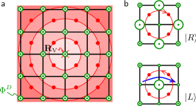
Figure 3: Vortex Hamiltonian. (a) The vortex hops between dual lattice sites (red), where at half filling for the bosons the average dual flux per plaquette is $1\over 2$ a flux quantum. The circular contours represent the equipotential contours for the confining potential for the vortex. When the Aharonov-Bohm fluxes are tuned to $\Theta_{x}^{0},\Theta_{y}^{0}$, the minimum of the potential is situated on a (direct) lattice site and the vortex ground state has two degenerate states $|R\rangle$, $|L\rangle$. (b) The two ground states correspond to two different charge density wave configurations, with $|R\rangle$ ($|L\rangle$) corresponding to depleted (excess) charge at ${\tenmib R}_{\rm V}$. When the particle hole symmetry breaking terms of Eq. (19) are introduced, hopping terms through ${\tenmib R}_{\rm V}$ (depicted by the blue arrow) lower the energy of the state $|L\rangle$ relative to $|R\rangle$.

If the point $\bf R_{\rm V}$ lies on a site of the direct lattice, the eigenstates of ${\cal H}_{\textsf{V}}$ (in a symmetric gauge) can be written as $\psi({\tenmib R}-{\tenmib R}_{\rm V})=f(\left|{\tenmib R}-{\tenmib R}_{\rm V}\right|)e^{im\varphi({\tenmib R}-{\tenmib R}_{\rm V})}$. Here $\varphi\left({\tenmib R}-{\tenmib R}_{\rm V}\right)$ denotes the angle between ${\tenmib R}-{\tenmib R}_{\rm V}$ and the $x$-axis, and $m=0,\pm 1,\pm 2$. At half filling, the average dual flux per plaquette is $\overline{\Phi}_{D}=\pi$ and the ground state is doubly degenerate with $m=0,1$. The two states $|R\rangle$ ($m=0$) and $|L\rangle$ ($m=1$) represent states with clockwise and counter-clockwise vortex currents, respectively, as depicted in Fig. 3(b). Note that this two-fold degeneracy occurs for $N$ distinct values of $\boldsymbol{\Theta}$.

To calculate $\sigma_{xy}$ we need to analyze the spectrum around the $N$ degeneracy points. Around these points, the Hamiltonian restricted to the $|R\rangle$ and $|L\rangle$ basis is of the form $H_{\rm V}={\bf h}\cdot{\boldsymbol{\sigma}}$ . To find ${\bf h}$, we first notice that if $\boldsymbol{\Theta}^{0}=\left(\Theta_{x}^{0},\Theta_{y}^{0}\right)$ is a degeneracy point, tuning away from it by $\boldsymbol{\Theta}=\boldsymbol{\Theta}^{0}+\Delta\boldsymbol{\Theta}$, moves ${\tenmib R}_{\rm V}$ as Lindner10

$${\tenmib R}_{\rm V}={\tenmib R}^{0}_{\rm V}+\Delta{\tenmib R}_{\rm V},\qquad\Delta R_{\rm V}^{\alpha}=-{\textstyle{1\over 2\pi}}\epsilon^{\alpha\beta}L_{\alpha}\Delta\Theta_{\beta},$$ (24)

where $\alpha,\beta=x,y$ and indices are not summed. Thus, tuning away from $\boldsymbol{\Theta}^{0}$ breaks the degeneracy between the two ground states $|R\rangle$ and $|L\rangle$, as it shifts the minimum of the potential $U({\tenmib R}-{\tenmib R}_{\rm V})$. Second, the terms $\propto\epsilon_{m}$ in (19) lift the degeneracy even at $\boldsymbol{\Theta}=\boldsymbol{\Theta}^{0}$; the assisted hopping terms through ${\tenmib R}_{\rm V}$ (blue arrow in Fig. 3) favor $|L\rangle$ over $|R\rangle$.

Together, these two effects give rise to the following low energy Hamiltonian for each degeneracy point (see supplementary materials for details),

$${\cal H}_{\textsf{V}}=\tilde{U}\left(-\Delta\Theta_{y}\sigma_{x}+\Delta\Theta_{x}\sigma_{y}\right)+\tilde{\epsilon}\sigma_{z}.$$ (25)

where the energy scales appearing above are $\tilde{U}\propto{\textstyle{\partial U\over\partial{{\tenmib R}}}}{\textstyle{L_{\alpha}\over 2\pi}}$, and $\tilde{\epsilon}\propto\epsilon_{m}$.

We use Eqs. (21-25) to calculate the Hall conductivity for one vortex. Consider the Hamiltonian ${\cal H}_{\scriptscriptstyle\rm HC}^{(1)}$ of Eq. (19) where we let the parameter $\epsilon_{m}$ take on both negative and positive values. For $0<\epsilon_{m}/t\ll 1$, the many body ground state $\Psi_{+}(\boldsymbol{\Theta},\epsilon_{m})$ is non-degenerate, and likewise $\Psi_{-}(\boldsymbol{\Theta},\epsilon_{m})$ for $-1\ll\epsilon_{m}/t<0$. For $\epsilon_{m}=0$ the two states become degenerate at a set of $N$ values of $\boldsymbol{\Theta}$ space. The Berry connection of the ground state manifold at $\epsilon_{m}=0$ is given by

$${\cal A}_{\mu}=i\sum_{i=+,-}\left\langle{\Psi_{i}(\boldsymbol{\Theta})}\bigg{|}{\partial\Psi_{i}(\boldsymbol{\Theta})\over\partial\Theta^{\vphantom{*}}_{\mu}}\right\rangle$$ (26)

and must satisfy $\int d^{2}\boldsymbol{\Theta}\,{\cal F}=0$ due to particle hole symmetry at $\epsilon_{m}=0$. As a result,

$$\sigma_{xy}(\epsilon_{m}>0)+\sigma_{xy}(\epsilon_{m}<0)=0$$ (27)

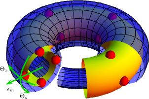
Figure 4: Berry monopoles. The parameter space of $\Theta_{x}$,$\Theta_{y}$, and $\epsilon_{m}$. The yellow surface denotes the particle-hole symmetric manifold $\epsilon_{m}=0$, on which the red dots denote the degeneracy points for $N$ values of $(\Theta_{x},\Theta_{y})$. The blue surfaces denote $\epsilon_{m}<0$ and $\epsilon_{m}>0$. The integral of the curvature ${\cal F}$ on these surfaces counts the number of sources in the three dimensional parameter space which they enclose.

Next, we consider the space of $\Theta_{x},\Theta_{y},\epsilon_{m}$, which has the topology of a thick torus, as depicted in Fig. 4. We are interested in the integral of the Berry curvature ${\cal F}$ on the surfaces with $\epsilon_{m}>0$ and $\epsilon_{m}<0$, which yield $\sigma_{xy}(\epsilon_{m}>0)$ and $\sigma_{xy}(\epsilon_{m}<0)$ respectively. At the same time, an analog of Gauss’ law for ${\cal F}$ implies that the integral of ${\cal F}$ on these surfaces counts the number of sources for ${\cal F}$ Berry84 ; Simon83 . These are just the degeneracy points discussed above, which are all described by Eq. (25) and therefore correspond to sources with charge $+\mbox{$1\over 2$}$. This leads to

$$\sigma_{xy}(\epsilon_{m}>0)-\sigma_{xy}(\epsilon_{m}<0)=N.$$ (28)

Combining Eqs. (27) and (28) gives

$$\sigma_{xy}(0<t/U\ll 1)={\textstyle{N\over 2}}.$$ (29)

Before concluding this section, we note that Eq. (24) leads to an exact relation between $\alpha$ and the Hall conductivity of one vortex. From Eq. (24), the Berry phase for moving a vortex around a plaquette is given by

$$2\pi\alpha=\oint_{\cal C}d\Theta_{\mu}\,{\cal A}_{\mu}=\int_{S({\cal C})}d^{2}\boldsymbol{\Theta}\,{\cal F}$$ (30)

where the contour ${\cal C}$ defines a square of size $2\pi/L_{x}\times 2\pi/L_{y}$ in flux space, and $S({\cal C})$ is the surface it bounds. Therefore, for one vortex,

$$\alpha N={\textstyle{1\over 2\pi}}\int\limits_{0}^{2\pi}\!\!d\Theta^{\vphantom{*}}_{x}\!\!\int\limits_{0}^{2\pi}\!\!d\Theta^{\vphantom{*}}_{y}\,{\cal F}=\sigma_{xy}.$$ (31)

Consider again the phase diagram of the Bose Hubbard model. From the above discussion, we conclude that the transitions lines between two integer values for $p$ emanate from the HCB points, and move to higher densities with increasing $t/U$. These lines all correspond to changes of the integer $p$ by unity. The PHS lines emanating from the neighboring Mott lobe tips terminate at the transition lines, cf. Fig. 1. Together, they define regions with negative $\alpha$ and Hall conductivity.

V Evolution of the transition lines

We numerically calculate the Chern number (21) for one vortex, to obtain the behavior of the integer $p$ in the full parameter regime of the Bose Hubbard model. We use a Lanczos algorithm Albuquerque07 to find the ground-state wave function $\Psi_{0}(\boldsymbol{\Theta})$ for different AB fluxes. Using a standard procedure Fukui05 to numerically integrate the Berry curvature (22) we obtain the Hall conductivity for different values of $t/U$ and $n_{b}$.

In Fig. 5 we show the results obtained for a $3\times 3$ cluster, cf. supplementary materials. We indicate which integer $p$ describes the Hall conductivity in panel (b). Panel (a) shows a trace of $\sigma_{xy}$ for different particle numbers at $t/U=0.2$. In both panels the region in the phase diagram where $\sigma_{xy}<0$ are marked with yellow hatches. As expected from the calculation at half-filling, the transition lines between two integer value of $p$ move to higher densities for $t/U>0$. Remarkably, the transition lines intersect the integer density line at increasing values of $t/U$ for higher densities. As a direct consequence the area of negative Hall conductivity increases for higher densities. This is in contrast to the decreasing extent of the Mott insulating phases indicated by the yellow bars in Fig. 5(b). This surprising behavior of the Bose-Hubbard model is explained below.

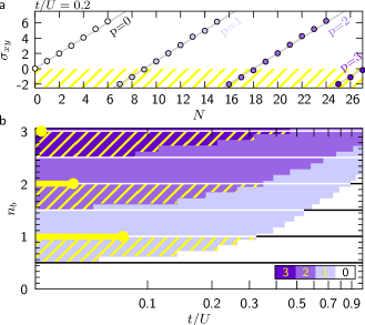
Figure 5: Numerical results. (a) The Chern number calculated numerically on a $3\times 3$ system at $t/U=0.2$ for various particle numbers $N$. The different branches are described by different integers $p$. The regions where the resulting Hall conductivity is negative is hatched in yellow. (b) Phase diagram obtained from cuts of the form of panel (a). Different colors indicate the different integers $p$. The lines where the integer $p$ changes by one are the topological transitions. The Mott insulators at integer filling are indicated by the yellow bars.

In order to see at which values of $t/U$ a sign change of $\alpha$ should be expected at integer fillings, we consider the healing length $\xi_{\scriptscriptstyle\rm GPE}$, which sets the size of a vortex. For $\xi_{\scriptscriptstyle\rm GPE}=a\sqrt{t/Un_{b}}\ll a$ the size of a vortex is much smaller then the lattice spacing $a$ Huber08 , and the Bose Hubbard model maps onto the quantum rotor model Simanek80 ; Doniach81 which has an emergent PHS at integer filling Fisher91 ; Sonin97 . We have seen that PHS implies $\alpha=0$. The dependence of $\xi_{\scriptscriptstyle\rm GPE}$ on the mean-field interaction $Un_{b}$ therefore explains the growing extent of the negative Hall conductivity. This has to be contrasted to the bosonic enhancement factors in the hopping terms $\propto\sqrt{n_{b}}$ which facilitate the melting of the Mott insulator and lead to smaller Mott lobes at increasing densities.

Finally, in Fig. 1 we present the numerical results as a function of $t/U$ and $\mu/U$. To translate from the results at fixed density $n_{b}$ to a fixed chemical potential $\mu$ we use a standard mean-field approach Huber07 .

VI Experimental verification

Our results have a direct experimental signature in terms of the vortex flow velocity in a moving system of lattice bosons. If $\sigma_{xy}$ is positive (negative) the vortices move with (against) the superfluid flow, cf. Eq. (3).

In a cold-atoms setup, the direction and speed of the vortex flow can be measured with in-situ imaging techniques Bakr09 . However, in the strongly interaction regime the vortex core is smaller then a lattice spacing $a$. Hence, to make the vortex visible in the density profile, the system parameters have to be ramped into the weakly interaction regime before imaging.

The sign change of the Hall conductivity can also be measured studying collective modes in a trap. When the atom cloud is displaced from the minimum of the harmonic trap the atoms start to oscillate in the trap Jin96 . A non-vanishing $\sigma_{xy}$ induces a transverse force on this dipole mode leading to a rotation of the axis of oscillation. Depending on the sign of the Hall conductivity the rotation is clock or counter-clockwise.

VII Discussion and outlook

In this paper we focused on vortex dynamics for the Bose-Hubbard model. We mapped the sectors corresponding to different integer $p$ which characterizes the Hall conductivity and vortex motion throughout the phase diagram. We found that close to the Mott insulating phases the sign of $\sigma_{xy}$ is reversed and vortices flow against the applied current.

Our results are obtained neglecting vortex-vortex interactions or disorder. We note, however, that there are an infinite number of particle hole symmetric points in the zero temperature phase diagram: at the tip of every Mott lobe, and in between two adjacent Mott lobes. We saw that the latter necessarily slice the full phase diagram into an infinite number of different $p$-sectors. This underlying structure cannot be removed by the inclusion of vortex-vortex interactions or disorder. However, the transition lines are expected to change their exact location and to be smoothed out by these effects, as well as by finite temperature.

Incidentally, reversal of the Hall conductivity have been repeatedly measured in many strongly correlated electronic materials, including high temperature superconductors, e.g. in Refs. Hagen90 ; LeBoeuf07 ; LeBoeuf11 . These experiments are beyond the direct applicability of our model. An extension to treat these materials is an interesting future direction. As discussed above, a clean verification of our predictions is possible in systems of cold atoms.

Acknowledgement

We thank Assa Auerbach, Ehud Altman, Joseph Avron, Hans-Peter Büchler, Olexi Motrunich, and Ady Stern for fruitful discussions. Special thanks to Daniel Podolsky for his enlightening comments. NHL acknowledges support by the Gordon and Betty Moore Foundation through Caltech’s Center for the Physics of Information, National Science Foundation Grant No. PHY-0803371, and the Israel Rothschild foundation. SDH acknowledges support by the Swiss Society of Friends of the Weizmann Institute of Science. This research was supported in part by the National Science Foundation under Grant No. PHY05-51164.

Appendix A Vortex translation operators

We derive the commutation relations for the vortex translation operators

$${\cal T}_{x}{\cal T}_{y}={\cal T}_{y}{\cal T}_{x}\exp(2\pi i\hat{N}_{b}/N)$$ (32)

Our derivation of equations (32) holds for any interaction strength $U$ in the Bose Hubbard model (5). We consider the Hamiltonian of Eq. (5) on a torus with $N=L_{x}L_{y}$ sites. The gauge field $A_{{\tenmib r}{\tenmib r}^{\prime}}$ describes one flux quantum piercing the surface of the torus uniformly, whereby the flux per plaquette is given by

$$B={\textstyle{2\pi\over L_{x}L_{y}}}.$$ (33)

An important gauge invariant quantity described by the gauge field ${\bf A}$ are the Wilson loop functions

$$\Phi_{x}(y)=\oint dxA_{x},\qquad\Phi_{y}(x)=\oint dyA_{y}.$$ (34)

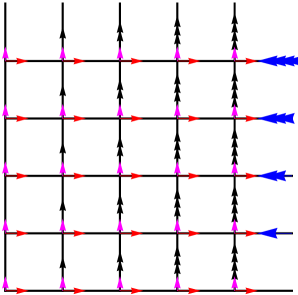
Figure 6: The gauge choice Eq. (35). Arrows on links represent the values for $A_{{\tenmib r},{\tenmib r}^{\prime}}$: Black arrows represent a value of $B$, blue arrows represent $BL_{x}$, red represent $\Theta_{x}/L_{x}$, and magenta $\Theta_{y}/L_{y}$. Open links stand for periodic boundary conditions.

We choose a continuous parametrization of the gauge field, which yields a continuous family of Wilson line function. Our gauge choice is given by

$$A^{x}_{{\tenmib r},{\tenmib r}+\hat{{\tenmib x}}} = yBL_{x}\delta_{x,L_{x}-1}+{\textstyle{\Theta_{y}\over L_{x}}}$$

$$A^{y}_{{\tenmib r},{\tenmib r}+\hat{{\tenmib y}}} = xBL_{x}+{\textstyle{\Theta_{x}\over L_{y}}}.$$ (35)

where $x=0,...,L_{x}-1$, and $y=0,...,L_{y}-1$. Our gauge choice is shown in Fig. 6. The two Wilson loop functions are given by

$$\Phi^{\vphantom{*}}_{y}(x) = \phantom{-}xBL_{y}+\Theta^{\vphantom{*}}_{y},$$ (36)

$$\Phi^{\vphantom{*}}_{x}(y) = -yBL_{x}+\Theta^{\vphantom{*}}_{x}.$$ (37)

Note that the parameters $\Theta_{x},\Theta_{y}\in\left[0,2\pi\right]$ define a continuous family of Hamiltonians, which are inequivalent under gauge transformation.

Let $t_{x}$ and $t_{y}$ be lattice translation operators, i.e.

$$t_{x}^{{\dagger}}b_{{\tenmib r}}t_{x}=b_{{\tenmib r}+\hat{\bf x}},\qquad t_{y}^{{\dagger}}b_{{\tenmib r}}t_{y}=b_{{\tenmib r}+\hat{\bf y}}$$ (38)

Translating the Hamiltonian by $t_{x}$ and $t_{y}$ leads to

$$t_{\alpha}^{\dagger}{\cal H}[{\tenmib A}]t_{\alpha} = {\cal H}[\tilde{{\tenmib A}}^{(\alpha)}],$$

$$\tilde{A}^{(\alpha)}_{{\tenmib r},{\tenmib r}^{\prime}} = A_{t_{\alpha}({\tenmib r}),t_{\alpha}({\tenmib r}^{\prime})}.$$ (39)

The gauge invariant content of the new gauge fields $\tilde{{\tenmib A}}^{(\alpha)}$ is the same flux per plaquette $B$ as for ${\tenmib A}$, however the Wilson line functions of Eq. (34) are shifted by one lattice constant,

$$t_{x}:\Phi_{y}(x)\to\tilde{\Phi}_{y}(x) = \Phi_{y}(x+1)$$

$$t_{y}:\Phi_{x}(y)\to\tilde{\Phi}_{x}(y) = \Phi_{x}(y+1).$$ (40)

Note that the values of the Wilson lines cannot be changed by a gauge transformation. Therefore if we conjugate the Hamiltonian by $t_{x}$ or $t_{y}$ we cannot make a gauge transformation back to the original Hamiltonian. However, we can find gauge transformations $U_{x}$ and $U_{y}$ that yield the following relations:

$$U_{\alpha}^{{\dagger}}t_{\alpha}^{{\dagger}}{\cal H}\left[{\tenmib A}(\boldsymbol{\Theta})\right]t_{\alpha}U_{\alpha}^{{\dagger}}={\cal H}\left[{\tenmib A}\left(\boldsymbol{\Theta}-\Delta\boldsymbol{\Theta}^{(\alpha)}\right)\right],$$ (41)

where $\boldsymbol{\Theta}=(\Theta_{x},\Theta_{y})$, and

$$(\Delta\Theta^{(\alpha)})_{\beta}=\epsilon^{\alpha\beta}BL_{\beta}.$$ (42)

where $\epsilon^{\alpha\beta}$ is an antisymmetric tensor with $\epsilon^{xy}=1$.

We parametrize the unitaries $U_{x}$ and $U_{y}$ as

$$U_{x}=\exp(i2\pi\sum_{\tenmib r}\chi^{x}_{\tenmib r}\,b^{{\dagger}}_{\tenmib r}b_{\tenmib r}),\quad U_{y}=\exp(i2\pi\sum_{\tenmib r}\chi^{y}_{\tenmib r}\,b^{{\dagger}}_{\tenmib r}b_{\tenmib r}),$$

where the functions $\chi^{\alpha}_{\tenmib r}$ are given by

$$\chi^{\alpha}_{\tenmib r}=\int^{{\tenmib r}}d{\tenmib r}^{\prime}\cdot\left({\tenmib A}(\boldsymbol{\Theta}-\Delta\boldsymbol{\Theta}^{(\alpha)})-\tilde{{\tenmib A}}^{(\alpha)}\right).$$ (43)

We now calculate the commutation relation between ${\cal T}_{x}$ and ${\cal T}_{y}$. An explicit formula for $\chi^{\alpha}_{\tenmib r}$ using the gauge choice Eq. (35) reads

$$\chi^{x}({\tenmib r}) = -BL_{x}y\delta_{x,0},$$

$$\chi^{y}({\tenmib r}) = \phantom{-}Bx.$$ (44)

Multiplying these operators we get

$${\cal T}_{y}{\cal T}_{x} = t_{y}t_{x}\exp\left(i\sum_{\tenmib r}\left(\chi^{x}_{\tenmib r}+\chi^{y}_{{\tenmib r}-{\tenmib x}}\right)\,b^{{\dagger}}_{\tenmib r}b_{\tenmib r}\right),$$

$${\cal T}_{x}{\cal T}_{y} = t_{x}t_{y}\exp\left(i\sum_{\tenmib r}\left(\chi^{x}_{{\tenmib r}-{\tenmib y}}+\chi^{y}_{{\tenmib r}}\right)\,b^{{\dagger}}_{\tenmib r}b_{\tenmib r}\right)$$ (45)

$$= {\cal T}_{y}{\cal T}_{x}\exp(i\Upsilon).$$

In the above equation, we have used $\left[t_{x},t_{y}\right]=0$. The factor $\exp(i\Upsilon)$ is given by

$$\Upsilon=\sum_{\tenmib r}\omega_{\tenmib r}\,b^{{\dagger}}_{\tenmib r}b_{\tenmib r},$$ (46)

with

$$\omega_{\tenmib r}=\chi^{x}_{\tenmib r}-\chi^{x}_{{\tenmib r}-{\tenmib y}}+\chi^{y}_{{\tenmib r}-{\tenmib x}}-\chi^{y}_{{\tenmib r}}.$$ (47)

Using Eq. (44) we get

$$\omega_{\tenmib r}=-B,$$ (48)

and substituting this into Eq. (45) we arrive at our final result

$${\cal T}_{x}{\cal T}_{y}={\cal T}_{y}{\cal T}_{x}\exp(2\pi i\hat{N}_{b}/N).$$ (49)

Here, $\hat{N}_{b}$ is the boson number operator and $N$ are the number of sites.

Note that although explicit gauge choice were made in the derivation of Eq. (32),the result is gauge invariant: a different gauge choice in Eq. (32) yield the same result.

To relate ${\cal T}_{x}$ and ${\cal T}_{y}$ to the vortex position, we note that the vortex position can only depend on the values the Wilson lines $\Phi_{x}(y)$ and $\Phi_{y}(x)$, as these the only gauge invariant quantities which break the translational symmetry on the torus. Therefore, the ground states of the continuous family of Hamiltonians ${\cal H}[{\tenmib A}(\boldsymbol{\Theta})]$ corresponds to many body states $\Psi(\Theta)$ with vortex positions continuously parametrized by $\boldsymbol{\Theta}$ as well. The vortex position in the many body states $\Psi(\boldsymbol{\Theta})$ has quantum fluctuations; the amplitudes however are centered around a point ${\tenmib R}_{\rm V}$ which depends only on $\boldsymbol{\Theta}$ Lindner09 ; Lindner10 . As a result, the action of ${\cal T}_{x}$ and ${\cal T}_{y}$ shifts the vortex position by one lattice site in the $x$ and $y$ direction accordingly.

To relate Eq. (49) to $2\pi\alpha$, the Berry phase acquired by moving a vortex around a dual lattice plaquette, we note that

$$\exp(i2\pi\alpha) = \exp(i\oint d\Theta_{\mu}{\cal A}_{\mu})$$ (50)

$$= \langle\Psi(\boldsymbol{\Theta}^{0})|U_{4}U_{3}U_{2}U_{1}|\Psi(\boldsymbol{\Theta}^{0})\rangle,$$

where ${\cal A}_{\mu}=i\langle\Psi(\boldsymbol{\Theta})|\partial_{\Theta_{\mu}}\Psi(\boldsymbol{\Theta})\rangle$, and the line integral is taken around a plaquette in flux space of size $\left(BL_{y},BL_{x}\right)$. In Eq. (50), $U_{i}=U(\boldsymbol{\Theta}^{i},\boldsymbol{\Theta}^{i+1})$ are adiabatic evolution operators from $\boldsymbol{\Theta}^{i}$ to $\boldsymbol{\Theta}^{i+1}$, and

$$\boldsymbol{\Theta}^{1} = \boldsymbol{\Theta}^{0}+\Delta\boldsymbol{\Theta}^{(x)}$$

$$\boldsymbol{\Theta}^{2} = \boldsymbol{\Theta}^{0}+\Delta\boldsymbol{\Theta}^{(x)}+\Delta\boldsymbol{\Theta}^{(y)}$$

$$\boldsymbol{\Theta}^{3} = \boldsymbol{\Theta}^{0}+\Delta\boldsymbol{\Theta}^{(y)}$$

$$\boldsymbol{\Theta}^{4} = \boldsymbol{\Theta}^{0}.$$

Using $U_{3}={\cal T}_{y}U_{1}^{{\dagger}}{\cal T}_{y}^{\dagger}$ and $U_{4}={\cal T}_{x}^{\dagger}U_{2}^{{\dagger}}{\cal T}_{x}$ and assuming that the ground state $|\Psi(\boldsymbol{\Theta})\rangle$ is non-degenerate, we find

$$\exp(i\oint d\Theta_{\mu}{\cal A}_{\mu}) = \langle\Psi(\boldsymbol{\Theta}^{0})|{\cal T}^{{\dagger}}_{y}{\cal T}^{{\dagger}}_{x}{\cal T}_{y}{\cal T}_{x}|\Psi(\boldsymbol{\Theta}^{0})\rangle$$ (52)

$$= \exp(-i2\pi n_{b})$$

Finally, from Eq. (52) we see that the Berry flux through an elementary plaquette in flux space (which has the topology of a torus) is $2\pi(n_{b}+p)$. All of the $N$ elementary plaquette on the flux torus are identical. The Hall conductivity is given by the integral of the Berry curvature on the whole flux torus Avron85 , and therefore, in the presence of one vortex,

$$\sigma_{xy}=N(n_{b}+p).$$ (53)

Appendix B Vortex hopping Hamiltonian

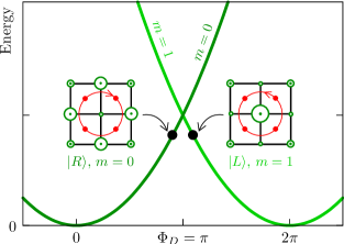
Figure 7: Vortex Hamiltonian. The green curves show the energy for a particle on a ring as a function of the flux through its center. At slightly higher (lower) flux than $\Phi_{D}=\pi$ the state $m=1$ ($m=0$) is the ground state. Two charge density waves centered at ${\tenmib R}_{\rm V}$ lead to $\Phi_{D}=\pi+\delta,\pi-\delta$ and correspond to the states $|L\rangle$, $|R\rangle$ which have the same energy. Therefore, the state $|L\rangle$ ($m=1$) corresponds to a charge density wave with excess density at the center site.

In the following we derive the form of Hamiltonian (25). Let us start with the terms arising from a change in the AB fluxes $\boldsymbol{\Theta}=\boldsymbol{\Theta}^{0}+\Delta\boldsymbol{\Theta}$, which moves the vortex potential $U({\tenmib R}-{\tenmib R}_{\rm V})$ minimum according to (24). We can now apply degenerate perturbation theory in the subspace of $|R\rangle$ and $|L\rangle$. The effect of $\Delta\boldsymbol{\Theta}$ only leads to off diagonal matrix elements between $|R\rangle$ and $|L\rangle$ since both states have the same $|\psi({\tenmib R}-{\tenmib R}_{\rm V})|$ and the perturbation is diagonal with respect to ${\tenmib R}$. The state $|R\rangle+e^{-i\varphi}|L\rangle$ has excess weight along $\arctan(x/y)=\varphi$, and therefore becomes the ground state for $\Delta{\tenmib R}_{\rm V}$ along that direction, i.e.,

$${\cal H}_{\textsf{V}}=\tilde{U}\left(-\Delta\Theta_{y}\sigma_{x}+\Delta\Theta_{x}\sigma_{y}\right).$$ (54)

We now consider the effect of the particle-hole symmetry breaking terms of Eq. (19). We expect the two ground states $|R\rangle$ and $|L\rangle$ to conform to two charge density wave orders centered at ${\tenmib R}_{\rm V}$, as the moving vortex exerts a force on the particles due to the Josephson relation. We note that the two charge density wave orders decay exponentially with the distance from ${\tenmib R}_{\rm V}$ (the decay length scale is the lattice constant) Lindner09 ; Lindner10 . To see which of the states ($|R\rangle$ or $|L\rangle$) has an excess (reduced) density at ${\tenmib R}_{\rm V}$, we consider an analogy with a particle hopping on a ring around ${\tenmib R}_{\rm V}$.

In Fig. 7 we show the energy of a particle on a ring for the two states $|R\rangle$ with $m=0$ and $|L\rangle$ with $m=1$ as a function of the flux $\Phi_{D}$ through the center of the ring. Note that the energy of $|R\rangle$ for $\Phi_{D}=\pi-\delta$ is equal to that of $|L\rangle$ for $\Phi_{D}=\pi+\delta$ (at $\Phi_{D}=\pi$ the two states are degenerate). Consider now the vortex Hamiltonian of Eq. (23). At half filling for HCBs, we can consider two dual flux configurations which at ${\tenmib R}_{\rm V}$ have $\Phi_{D}({\tenmib R}_{\rm V})=\pi\pm\delta$. Via $\Phi_{D}({\tenmib r})=2\pi\langle S^{z}_{\tenmib r}+\mbox{$1\over 2$}\rangle$ they are related to two corresponding charge configurations (the two configurations are related by charge conjugation). From the analogy to the particle on a ring, we can infer that these two charge configurations lead to the vortex ground states $|L\rangle$, $|R\rangle$ respectively. We therefore conclude that the state $|L\rangle$ ($|R\rangle$) has an excess (reduced) density at ${\tenmib R}_{\rm V}$, respectively, cf. Fig. 7.

While for the particle-hole symmetric point these charge configurations are equivalent energetically, the assisted hopping ($t^{2}/U$) terms in Eq. (19) give different energies for the two configurations. Due to the exponential decay of the charge density wave order Lindner09 ; Lindner10 , the difference between the expectation value of these terms in the states $|L\rangle$, $|R\rangle$ is also going to decay exponentially with the distance to ${\tenmib R}_{\rm V}$.

To account for their effect we estimate the energy change using mean field HCBs states for $|L\rangle$, $|R\rangle$ of the form $|\Psi\rangle=\prod_{{\tenmib r}}|\psi_{{\tenmib r}}(\vartheta_{{\tenmib r}})\rangle$, with

$$|\psi(\vartheta_{{\tenmib r}})\rangle=\cos(\vartheta_{{\tenmib r}})|\downarrow\rangle+\sin(\vartheta_{{\tenmib r}})e^{i\varphi_{\tenmib r}}|\uparrow\rangle.$$ (55)

Here $\varphi_{\tenmib r}$ is the phase arising due to the votex. Due to the exponential decay of the charge density wave order we only consider the $3\times 3$ cluster shown in Fig. 7. We evaluate the assisted hopping (19) in a state where the parameters $\vartheta_{{\tenmib r}}$ are chosen such that the center site has $n_{b}=\mbox{$1\over 2$}\pm\delta$, its nearest neighbors $n_{b}=\mbox{$1\over 2$}\mp\delta/4$, and the sites at the corners of the cluster have $n_{b}=\mbox{$1\over 2$}$. We find that the energy difference is dominated by assisted hopping terms which hop over the central site ${\tenmib R}_{\rm V}$

$$E(|L\rangle)-E(|R\rangle)\approx-\epsilon_{m}\sum_{{\tenmib r},{\tenmib r}^{\prime}}\bigg{[}\langle L|e^{iA_{{\tenmib r}{\tenmib r}^{\prime}}}S^{+}_{\tenmib r}(S^{z}_{{\tenmib R}_{\rm V}}+\mbox{$1\over 2$})S^{-}_{{\tenmib r}^{\prime}}|L\rangle\\ -\langle R|e^{iA_{{\tenmib r}{\tenmib r}^{\prime}}}S^{+}_{\tenmib r}(S^{z}_{{\tenmib R}_{\rm V}}+\mbox{$1\over 2$})S^{-}_{{\tenmib r}^{\prime}}|R\rangle\bigg{]}$$ (56)

where ${\tenmib r}$ and ${\tenmib r}^{\prime}$ are nearest neighbors of ${\tenmib R}_{\rm V}$. As discussed above, the state $|L\rangle$ corresponds to higher density at ${\tenmib R}_{\rm V}$, therefore the quantity above is negative.

The combined effect of moving the vortex position ${\tenmib R}_{\rm V}$ away from a direct lattice site and the PHS symmetry breaking terms of (19) leads to the low energy effective Hamiltonian near the degeneracy point

$${\cal H}_{\textsf{V}}=\tilde{U}\left(-\Delta\Theta_{y}\sigma_{x}+\Delta\Theta_{x}\sigma_{y}\right)+\tilde{\epsilon}\sigma_{z},$$ (57)

which is given in Eq. (25).

Appendix C Exact diagonalization

We calculate the ground state wave function for different AB fluxes using the ALPS Lanczos application Albuquerque07 on a $3\times 3$ cluster. We choose the same gauge choice a depicted in Fig. 6. To obtain the phase diagram we truncate the local Hilbert-space to include all occupation states up to five particles per site.

To get some insight into finite size effects we also calculate $\sigma_{xy}$ for a $3\times 4$ cluster at filling $n_{b}=1$. To compare the two cluster sizes we estimate the Mott transition by considering the gap to the first excited state. We attribute the transition to a kink in the gap as a function of $t/U$. If we rescale the results for the Hall conductivity by the critical $t/U$ the change from $\sigma_{xy}=0$ to $\sigma_{xy}=1$ obtained with the two clusters fall on top of each other.

References

- (1) Ziman, J. M. Principles of the theory of solids (Cambridge University Press, London, 1972).
- (2) Wen, X.-G. Topological orders and edge excitations in fractional quantum hall states. Adv. in Phys. 44, 405 (1995).
- (3) Hagen, S. J., Lobb, C. J., Greene, R. L., Forrester, M. G. & Kang, J. H. Anomalous hall effect in superconductors near their critical temperatures. Physical Review B 41, 11630 (1990).
- (4) LeBoeuf, D. et al. Electron pockets in the fermi surface of hole-doped high-tc superconductors. Nature 450, 533–536 (2007).
- (5) LeBoeuf, D. et al. Lifshitz critical point in the cuprate superconductor yba2cu3oy from high-field hall effect measurements. Physical Review B 83, 054506 (2011).
- (6) Jaksch, D., Bruder, C., Cirac, J. I., Gardiner, C. W. & Zoller, P. Cold bosonic atoms in optical lattices. Phys. Rev. Lett. 81, 3108 (1998).
- (7) Jaksch, D. & Zoller, P. The cold atom hubbard toolbox. Annals of Physics 315, 52–79 (2005).
- (8) Fazio, R. & van der Zant, H. Quantum phase transitions and vortex dynamics in superconducting networks. Phys. Rep. 355, 235 (2001).
- (9) Simanek, E. Effect of charging energy on transition temperature of granular superconductors. Solid State Comm. 31 (1979).
- (10) Doniach, S. Quantum fluctuations in two-dimensional superconductors. Phys. Rev. B 24, 5063 (1981).
- (11) Uemura, Y. J. et al. Universal correlations between tc and ns/m∗ (carrier density over effective mass) in high-tc cuprate superconductors. Physical Review Letters 62, 2317 (1989).
- (12) Micnas, R., Robaszkiewicz, S. & Kostyrko, T. Thermodynamic and electromagnetic properties of hard-core charged bosons on a lattice. Physical Review B 52, 6863 (1995).
- (13) Mihlin, A. & Auerbach, A. Temperature dependence of the order parameter of cuprate superconductors. Physical Review B 80, 134521 (2009).
- (14) Fisher, M. P. A., Weichman, P. B., Grinstein, G. & Fisher, D. S. Boson localization and the superfluid-insulator transition. Phys. Rev. B 40, 546–570 (1989).
- (15) Lin, Y. J., Compton, R. L., Jimenez-Garcia, K., Porto, J. V. & Spielman, I. B. Synthetic magnetic fields for ultracold neutral atoms. Nature 462, 628–632 (2009).
- (16) Cooper, N. R. Optical flux lattices for ultracold atomic gases. Physical Review Letters 106, 175301 (2011).
- (17) Fisher, M. P. A. Hall effect at the magnetic-field-tuned superconductor-insulator transition. Physica A 177, 553 (1991).
- (18) Haldane, F. D. M. & Wu, Y.-S. Quantum dynamics and statistics of vortices in two-dimensional superfluids. Physical Review Letters 55, 2887 (1985).
- (19) Ao, P. & Thouless, D. J. Berry’s phase and the magnus force for a vortex line in a superconductor. Physical Review Letters 70, 2158 (1993).
- (20) Oshikawa, M. Commensurability, excitation gap, and topology in quantum many-particle systems on a periodic lattice. Phys. Rev. Lett. 84, 1535 (2000).
- (21) Paramekanti, A. & Vishwanath, A. Extending luttinger’s theorem to fractionalized phases of matter. Phys. Rev. B 70, 245118 (2004).
- (22) Capogrosso-Sansone, B., Prokov’ef, N. & Svistunov, B. Phase diagram and thermodynamics of the three-dimensional bose-hubbard model. Phys. Rev. B 75, 134302 (2007).
- (23) van Oosten, D., van der Straten, P. & Stoof, H. T. C. Quantum phases in an optical lattice. Phys. Rev. A 63, 053601 (2001).
- (24) Polkovnikov, A., Altman, E., Demler, E., Halperin, B. & Lukin, M. D. Decay of superfluid currents in a moving system of strongly interacting boson. Phys. Rev. A 71, 063613 (2005).
- (25) Dorsey, A. T. Vortex motion and the hall effect in type-ii superconductors: A time-dependent ginzburg-landau theory approach. Phys. Rev. B 46, 8376 (1992).
- (26) Macdonald, A. H., Girvin, S. M. & Yoshioka, D. expansion for the hubbard-model. Phys. Rev. B 37, 9753 (1988).
- (27) Lindner, N., Auerbach, A. & Arovas, D. P. Vortex dynamics and hall conductivity of hard core bosons. Phys. Rev. B 82, 134510 (2010).
- (28) Avron, J. E. & Seiler, R. Quantization of the hall conductance for general, multiparticle schrödinger hamiltonians. Phys. Rev. Lett. 54, 259 (1985).
- (29) Lindner, N. H., Auerbach, A. & Arovas, D. P. Vortex quantum dynamics of two dimensional lattice bosons. Physical Review Letters 102, 070403 (2009).
- (30) Simon, B. Holonomy, the quantum adiabatic theorem, and berry’s phase. Physical Review Letters 51, 2167 (1983).
- (31) Berry, M. V. Quantal phase factors accompanying adiabatic changes. Proc. R. Soc. Lond. A 392, 45 (1984).
- (32) Albuquerque, A. et al. The alps project release 1.3: Open-source software for strongly correlated systems. J. of Magn. Magn. Materials 310, 1187 (2007).
- (33) Fukui, T., Hatsugai, Y. & Suzuki, H. Chern numbers in discretized brillouin zone: Efficient method of computing (spin) hall conductances. J. Phys. Soc. Jpn. 74, 1674 (2005).
- (34) Huber, S. D., Theiler, B., Altman, E. & Blatter, G. Amplitude mode in the quantum phase model. Phys. Rev. Lett. 100, 050404 (2008).
- (35) Simanek, E. Instability of granular superconductivity. Phys. Rev. B 22, 459 (1980).
- (36) Sonin, E. B. Magnus force in superfluids and superconductors. Phys. Rev. B 55, 485 (1997).
- (37) Huber, S. D., Altman, E., Büchler, H. P. & Blatter, G. Dynamical properties of ultracold bosons in an optical lattice. Phys. Rev. B 75, 085106 (2007).
- (38) Bakr, W. S., Gillen, J. I., Peng, A., Fölling, S. & Greiner, M. A quantum gas microscope for detecting single atoms in a hubbard-regime optical lattice. Nature 462, 74 (2009).
- (39) Jin, D. S., Ensher, J. R., Matthews, M. R., Wieman, C. E. & Cornell, E. A. Collective excitations of a bose-einstein condensate in a dilute gas. Phys. Rev. Lett. 77, 420 (1996).