Strain-induced interface reconstruction in epitaxial heterostructures

Abstract

We investigate in the framework of Landau theory the distortion of the strain fields at the interface of two dissimilar ferroelastic oxides that undergo a structural cubic-to-tetragonal phase transition. Simple analytical solutions are derived for the dilatational and the deviatoric strains that are globally valid over the whole of the heterostructure. The solutions reveal that the dilatational strain exhibits compression close to the interface which may in turn affect the electronic properties in that region.

I Introduction

Recent discoveries in material science related to several unexpected properties of epitaxial heterostructures made of different transition metal oxide (TMO) materials, bring in the forefront of interest the problem of interface reconstruction through the developement of spontaneous strain at the interface Ohtomo2002 ; Ohtomo2004 . Lattice distortion close to the interface is known to result in charge redistribution that leads to the formation of a two-dimensional electron gas (2DEG) and metallicity in that region Shibuya2004 ; Okamoto2006 ; Ishida2008 ; Wong2010 . Most of the TMOs of interest are ferroelastics that undergo structural transitions Salje1990 from a cubic/pseudocubic to a lower symmetry phase with decreasing temperature. Notably, heterostructures containing strontium titanate (SrTiO₃), a band-insulator oxide undergoing a cubic-to-tetragonal (CTT) structural transition at $T_{s}\sim 105~{}^{o}K$, exhibit extraordinary interfacial properties below $T_{s}$; metallicity Ohtomo2002 ; Shibuya2004 ; Seo2007 ; Wong2010 , superconductivity Biscaras2010 , and nonlinear Hall effect Kim2010 . Moreover, in LaTiO₃/SrTiO₃ and LaAlO₃/SrTiO₃ heterostructures, the structural transition of SrTiO₃ causes the overlayers to stabilize in a tetragonal phase with an in-plane lattice constant almost equal to that of SrTiO₃ close to the interface Kim2003 ; Wu2011 .

It has been discussed in the past that the electromagnetic properties of TMOs couple to the elastic degrees of freedom Ahn2004 ; Bishop2008 ; Maniadis2008 . The effect of tensile and compressive strains to the electronic conduction properties at the interface of TMO heterostructures has already been addressed experimentally Bark2011 ; JWSeo2010 . Furthermore, strong polarization enhancement in ferroelectric TMO superlattices driven by interfacial strain has been unambigiously observed Lee2005 . In the present work we apply continuous elasticity theory through a Ginzburg-Landau description in terms of the strain tensor components to a heterostructure. Based solely on symmetry considerations, Ginzburg-Landau theory can provide a reliable description of the equilibrium behavior of a system near a phase transition. It has been recently used to show theoretically the emergence of a multiferroic state of a EuTiO₃ film on (LaAlO${}_{3})_{0.29}$–(SrAl_1/2Ta_1/2O${}_{3})_{0.71}$ (LSAT) substrate Lee2010 , to provide a physical understanding of the strain-induced metal-insulator phase coexistence in manganites Ahn2004 , and to explain phase separation between metallic ferromagnetic and insulating charge-modulated phases Milward2005 .

We investigate the interfacial effects on the strain-state of a bilayer heterostructure, composed of dissimilar TMOs that join at a single planar interface and propose a strain-based mechanism that may help understand the formation of a 2DEG. In particular, we obtain approximate analytical solutions for the dilatational and the deviatoric strain fields in the bilayer, that exhibit spatial variation due to breaking of the uniformity. Notably, the dilatational strain field exhibits a well-defined minimum at the interface corresponding to local compression Wong2010 . We argue that the suppression of the dilatational strain field in the interfacial region may encourage the formation of a 2DEG. The proposed strain-based mechanism does not exclude other possible mechanisms, like, e.g., the orbital and/or the electronic reconstruction mechanisms Chakhalian2007 ; Okamoto2004 .

II Ginzburg-Landau theory and equations of motion

In the Lagrangian description of elasticity the symmetric strain tensor is defined as $\epsilon_{ij}=\left\{u_{i,j}+u_{j,i}\right\}/2$ ($i,j=x,y,z$), where $u_{i,j}$ is the $j-$th derivative of the $i-$th component of the displacement vector $\bf u$ of a material point relative to its position in the parent phase. The six symmetry adapted strains for the CTT structural transition are defined as Jacobs2003

$$e_{1}=u_{x,x}+u_{y,y}+u_{z,z},~{}~{}e_{2}=\frac{1}{2}(u_{x,x}-u_{y,y})$$ (1)

$$e_{3}=\frac{1}{2\sqrt{3}}(u_{x,x}+u_{y,y}-2u_{z,z}),~{}~{}e_{4}=\frac{1}{2}(u_{y,z}+u_{z,y}),$$ (2)

while $e_{5}$ and $e_{6}$ are given by $e_{4}$ with cyclic permutation of the indices. The deviatoric strains $e_{2}$ and $e_{3}$ form the two-component order parameter (OP) of the CTT transition. Both the OP and the non-OP strains are coordinate-independent in the uniform product (tetragonal) phase in static equilibrium, with the latter customarily being set to zero. In a TMO heterostructure, where the uniformity of the product phase is broken due to the interface, all $e_{i}$’s vary spatially; in that case, their second derivatives are linked through compatibility relations Rasmussen2001 . In a non-uniform state, the non-OP strains cannot be all set to zero. Specifically, in TMO heterostructures the dilatational strain $e_{1}$, which is concommitant to $e_{3}$ Kosogor2011 ; Chernenko1996 , exhibits measurable compression indicating its importance in their structural properties Wong2010 .

In ferroelasticity theory, the strain energy density ${\cal F}$ of a material undergoing a CTT structural transition is expanded in powers of the invariants of the strain tensor and their products around the energy of the parent phase Kosogor2011 ; Chernenko1996 ; Barsch1984 ; Gomonaj1994 ; Gomonaj1996 ; Rasmussen2001 . Thus, the functional ${\cal F}$ is expressed solely in terms of the $e_{i}$’s and their spatial derivatives. Guided by previous works we adopt a functional ${\cal F}$ of the form

$${\cal F}=\frac{c_{1}}{2}e_{1}^{2}+\frac{c_{2}}{2}(e_{2}^{2}+e_{3}^{2})+\frac{c_{3}}{2}(e_{4}^{2}+e_{5}^{2}+e_{6}^{2})$$

$$+\frac{d_{1}}{2}\left({\bf\nabla}e_{1}\right)^{2}+\frac{d_{2}}{2}\left[\left({\bf\nabla}e_{2}\right)^{2}+\left({\bf\nabla}e_{3}\right)^{2}\right]$$

$$+\frac{a_{1}}{2}e_{1}^{3}+\frac{a_{2}}{2}e_{1}(e_{2}^{2}+e_{3}^{2})+\frac{a_{4}}{3}e_{3}(e_{3}^{2}-3e_{2}^{2})+\frac{b_{1}}{4}e_{1}^{4}$$

$$+\frac{b_{2}}{2}e_{1}^{2}(e_{2}^{2}+e_{3}^{2})+\frac{b_{4}}{4}(e_{2}^{2}+e_{3}^{2})^{2}+\frac{b_{7}}{2}e_{1}e_{3}(e_{3}^{2}-3e_{2}^{2}),$$ (3)

where the Ginzburg-Landau coefficients $a_{1},a_{2},a_{4}$, $b_{1},b_{2},b_{4},b_{7}$, and $c_{1},c_{2},c_{3}$ are related to the second-, third-, and fourth-order elastic coefficients of the parent phase, respectively, through (in Voigt notation) Liakos1982

$$a_{1} = \frac{1}{27}\left(C_{111}+6C_{112}+2C_{123}\right)$$

$$a_{2} = \frac{2}{3}(C_{111}-C_{123})$$

$$a_{4} = -\frac{1}{\sqrt{3}}\left(C_{111}-3C_{112}+2C_{123}\right)$$

$$b_{1} = \frac{1}{162}(C_{1111}+8C_{1112}+6C_{1122}+12C_{1123})$$

$$b_{2} = \frac{1}{9}(C_{1111}+2C_{1112}-3C_{1123})$$ (4)

$$b_{4} = \frac{1}{3}(C_{1111}-4C_{1112}+3C_{1122})$$

$$b_{7} = -2\frac{\sqrt{3}}{27}(C_{1111}-C_{1112}-3C_{1122}+3C_{1123})$$

$$c_{1} = \frac{1}{3}(C_{11}+2C_{12})$$

$$c_{2} = 2(C_{11}-C_{12}),$$

while $d_{1},d_{2}$ are two independent strain-gradient coefficients. In accordance with common principles of Landau theory, the critical temperature dependence of the $c_{2}$ elastic constant, $c_{2}\propto(T-T_{s})$, is supposed to be true close to the transition point.

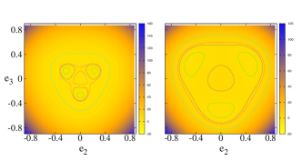
Figure 1: (color online) Strain energy density lanscape on the $e_{2}-e_{3}$ plane for $a_{4}=25.4$, $b_{4}=225$, and $c_{2}=-10$ (left); $-50$ (right), exhibiting the familiar pattern of three degenerate minima.

In a single material at static equilibrium, the spatially homogeneous strains in the product phase are the lowest energy solutions of the conditions ${\partial{\cal F}}/{\partial e_{i}}=0$. Neglecting the non-OP terms, the energy density landscape on the $e_{2}-e_{3}$ plane exhibits the familiar pattern of three degenerate minima corresponding to three different variants in the tetragonal phase (Fig. 1). Notably, a non-zero $e_{1}$ preserves the energetic degeneracy of the three variants. We are particularly interested in the variant having $e_{2}=0$; this is because TMO heterostructures are usually grown along the $z-$direction and both materials go into a $c-$tetragonal phase at low temperatures Kim2003 ; Wu2011 . For $e_{2}=0$, the energy landscape on the $e_{1}-e_{3}$ plane shown in Fig. 2 exhibits significant qualitative differences for different $a_{2}$ values. Specifically, the strain $e_{1}$ varies from positive (i.e., expansional) to negative (i.e., compressional) with decreasing the magnitude of $a_{2}$. A small $a_{2}$ absolute value is however expected from the principle $e_{1}<<e_{2},e_{3}$ for all martensitic transformations Gomonaj1994 ; Gomonaj1996 . Moreover, a small $a_{2}$ leads to negative $e_{1}$ and $e_{3}$, in accordance with the empirical principle for the ferroelastic transitions of close-packed solids, i.e., that cooling of the solid is usually accompanied by a decrease of volume. The dependence of the strains on $c_{2}$ for all three variants is shown in Fig. 3 for two different values of $a_{2}$. We later refer to the two materials forming the bilayer heterostructure, which occupy the regions $z<0$ and $z>0$, as the left ($L$) and the right ($R$) material, respectively. The Ginzburg-Landau parameters used in Figs. 1-3 are those given for the left material in Table I, and they have been calculated from the corresponding elastic coefficients through Eqs. (II). The second- and third-order elastic coefficients of the left material are those reported for SrTiO₃ Bell1963 ; Beattie1971 , while for the fourth-order ones a reasonable choise was made (Table I). Note that for the parameter $a_{2}$, which can be treated as a phenomenological one, we have also used values that are smaller than the one given in Table I for the left material (i.e., $a_{2}^{L}=-31$).

Figure 2: (color online) Strain energy density lanscape on the $e_{1}-e_{3}$ plane for $c_{2}=-50$, and $a_{2}=-31$ (left); $-10$ (right). The other Ginzburg-Landau parameters are those for the left material given in Table I.

The dynamics of the displacements is governed by the Euler-Lagrange equations

$$\rho_{0}\ddot{u}_{i}=\sigma_{ik,k}+\sigma_{ik,k}^{\prime},$$ (5)

where

$$\sigma_{ik}\equiv\frac{\partial{\cal F}}{\partial u_{i,k}},\qquad\sigma_{ik}^{\prime}\equiv\frac{\partial{\cal R}}{\partial\dot{u}_{i,k}},$$ (6)

are the strain tensor and the dissipative strain tensor, respectively, $\rho_{0}$ is the density in the parent phase, and ${\cal R}$ is the the Rayleigh dissipation function

$${\cal R}=\frac{1}{2}c_{1}^{\prime}\dot{e}_{1}^{2}+\frac{1}{2}c_{2}^{\prime}(\dot{e}_{2}^{2}+\dot{e}_{3}^{2})+\frac{1}{2}c_{3}^{\prime}(\dot{e}_{4}^{2}+\dot{e}_{5}^{2}+\dot{e}_{6}^{2}).$$ (7)

Then, from Eq. (5) we get

$$\rho_{0}\ddot{u}_{i}=\partial_{i}\Phi_{i}+\frac{1}{2}(c_{3}H_{i}+c_{3}^{\prime}\dot{H}_{i}),$$ (8)

where

$$H_{x}=e_{6,y}+e_{5,z},~{}H_{y}=e_{4,z}+e_{6,x},~{}H_{z}=e_{4,y}+e_{5,x},$$ (9)

and

$$\Phi_{i}=-\nabla^{2}G_{i}+W_{i}+R_{i}+\dot{W}_{i}^{\prime},$$ (10)

$$W_{i}=c_{1}e_{1}+\frac{c_{2}}{2}\left(qe_{2}+\frac{1}{\sqrt{3}}e_{3}\right),W_{z}=c_{1}e_{1}-\frac{c_{2}}{\sqrt{3}}e_{3},$$ (11)

with $q=+1~{}(-1)$ for $i=x~{}(y)$.

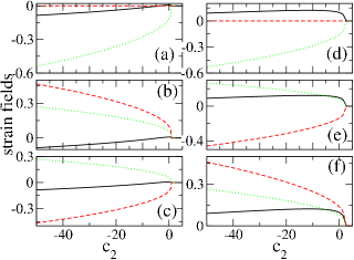
Figure 3: (color online) The strains $e_{1}$ (black-solid), $e_{2}$ (red-dashed), $e_{3}$ (green-dotted), as a function of $c_{2}$ for the three variants, for $a_{2}=-7$ (left panels); $-31$ (right panels). The other Ginzburg-Landau parameters are those for the left material given in Table I.

The functions $W_{i}^{\prime}$ and $G_{i}$ have the same form with that of the $W_{i}$’s, with the obvious change $c_{j}\rightarrow c_{j}^{\prime}$ and $c_{j}\rightarrow d_{j}$, respectivelly ($j=1,2$), and the $R_{i}$’s are lengthy nonlinear functions of $e_{1}$, $e_{2}$, and $e_{3}$, which are given in Appendix A.

III Approximate solutions and interface reconstruction

In order to separate the interfacial effects on the strain-state of the bilayer heterostructure (from those originating from external boundaries, domain walls, dislocations, etc.), we consider two monodomain, semi-infinite TMOs joined along a chemically abrupt, planar interface at $z=0$. Eqs. (8) could be simplified in a strict way, since at low temperatures the strains depend on one coordinate only and $e_{2}=0$ Chernenko2006 ; Chernenko2006b . However, for non-zero $e_{1}$ the simpification of Eqs. (8) following the strict way is a non-trivial task, which makes preferable the use of a simple ansatz for the displacements. This ansatz assures that the strains depend only on the $z-$coordinate and that $e_{2}$, as well as the small strains $e_{4}$, $e_{5}$, $e_{6}$, are identically zero. Assume that the strains exhibit a relatively strong $z-$coordinate dependence in the proximity of the interface, while they attain their static equilibium values for large enough $|z|$. This approximation seems well-suited for heterostuctures composed of TMOs with small lattice mismatch (i.e., LaTiO₃/SrTiO₃). Indeed, both experimental observations Helvoort2005 (discussed below) and first-principles calculations Okamoto2006 indicate that strain inhomogeneity and lattice deformation occur within a few layers near the interface. Thus, for practical purposes, it is sufficient for the two layers of the heterostructure to be thick enough for the deformation to vanish relatively far from the interface. The choise of semi-infinite layers was made only for mathematical convinience.

We then introduce the ansatz

$$u_{x}=-\frac{a}{2}x,~{}~{}~{}u_{y}=-\frac{a}{2}y,~{}~{}~{}u_{z}=bz+f(z),$$ (12)

where $f(z)$ is a yet unknown function, and

$$a=-\frac{2}{3}(e_{10}+\sqrt{3}e_{30}),\qquad b=+\frac{1}{3}(e_{10}-2\sqrt{3}e_{30}),$$ (13)

with $e_{10}$ and $e_{30}$ being the values of $e_{1}$ and $e_{3}$, respectively, far from the interface. The non-zero strains are then

$$e_{1}=e_{10}+f^{\prime}(z),\qquad e_{3}=e_{30}-\frac{1}{\sqrt{3}}f^{\prime}(z),$$ (14)

where the prime denotes differentiation with respect to $z$. Substitution of Eq. (14) into Eqs. (8) results, in the static limit, in the equation

$$\left(d_{1}+\frac{d_{2}}{3}\right)G^{\prime\prime\prime}=\left(c_{1}+\frac{c_{2}}{3}\right)G^{\prime}+R_{z}^{\prime}(G),$$ (15)

where $G=G(z)\equiv f^{\prime}(z)$, and $R_{z}$ with $e_{2}=0$ is

$$R_{z}=\frac{3a_{1}}{2}e_{1}^{2}+b_{1}e_{1}^{3}+\left(\frac{a_{2}}{2}-\frac{a_{4}}{\sqrt{3}}\right)e_{3}^{2}+\left(\frac{b_{7}}{2}-\frac{b_{4}}{\sqrt{3}}\right)e_{3}^{3}$$

$$-\frac{1}{\sqrt{3}}e_{1}e_{3}\left[a_{2}+b_{2}e_{1}+3\left(\frac{b_{7}}{2}-\frac{b_{2}}{\sqrt{3}}\right)e_{3}\right],~{}~{}~{}~{}~{}$$ (16)

where $e_{1}$ and $e_{3}$ are meant to be expressed in terms of $f$ through Eq. (14). After rearrangement, Eq. (15) becomes

$$G^{\prime\prime\prime}=G^{\prime}(\tilde{\kappa}+3\tilde{\lambda}G+6\tilde{\mu}G^{2}),$$ (17)

where

$$\tilde{\kappa}=\frac{a_{1z}+\kappa}{d_{1z}},~{}~{}\tilde{\lambda}=\frac{\lambda}{3d_{1z}},~{}~{}\tilde{\mu}=\frac{\mu}{6d_{1z}},$$ (18)

with

$$a_{1z}=c_{1}+\frac{1}{3}c_{2}=C_{11},\qquad d_{1z}=d_{1}+\frac{1}{3}d_{2},$$ (19)

and

$$\kappa = bC_{111}-3aC_{112}+\frac{3a^{2}}{4}(C_{1122}+C_{1123})-3abC_{1112}$$

$$+\frac{b^{2}}{2}C_{1111},$$

$$\lambda = c_{111}+(bC_{1111}-aC_{1112}),$$ (20)

$$\mu = \frac{1}{2}C_{1111}.$$

Eq. (17) can be reduced to a quadrature that has the analytic solution

$$G^{\pm}=4\tilde{\kappa}\left(e^{\pm\sqrt{\tilde{\kappa}}(z\mp z_{0})}+\Delta e^{\mp\sqrt{\tilde{\kappa}}(z\mp z_{0})}+\Delta_{1}\right)^{-1},$$ (21)

where $-\Delta\equiv 4\tilde{\kappa}\tilde{\mu}-\tilde{\lambda}^{2}$, $\Delta_{1}=-2\tilde{\lambda}$, and $z_{0}$ is a constant of integration. Integration of $G^{\pm}$ gives

$$f^{\pm}=\mp\frac{2}{\sqrt{\tilde{\mu}}}\tanh^{-1}\left(\frac{e^{\pm\sqrt{\tilde{\kappa}}(z\mp z_{0})}-\tilde{\lambda}}{2\sqrt{\tilde{\kappa}\tilde{\mu}}}\right)+C^{\pm},$$ (22)

where $C^{\pm}$ are constants of integration.

The displacements and the strains in each material of the bilayer can be written in terms of $f^{\pm}$ and $G^{\pm}$ from Eqs. (12) and (14), respectively.

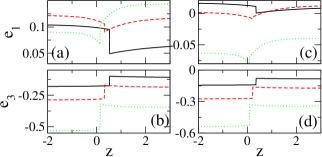
Figure 4: (color online) The strains $e_{1}$ and $e_{3}$ as a function of $z$ for $c_{2}^{L}=-1$, $c_{2}^{R}=-0.76$ (black-solid), $c_{2}^{L}=-10$, $c_{2}^{R}=-7.56$ (red-dashed); $c_{2}^{L}=-50$, $c_{2}^{R}=-37.8$ (green-dotted), and (a)-(b): $a_{2}^{L}=-31$, $a_{2}^{R}=-29.5$; (c)-(d): $a_{2}^{L}=-10$, $a_{2}^{R}=-9.5$. The other Ginzburg-Landau parameters are those for the left and the right material given in Table I.

Specifically, the solutions for $u_{z}$, $e_{1}$, $e_{3}$ in the material left, (right) from the interface occupying the region $z<0$ ($z>0$) are written as

$$u_{z}^{L(R)}=b^{L(R)}+f^{+(-)},$$ (23)

$$e_{1}^{L(R)}=e_{10}^{L(R)}+G^{+(-)},~{}~{}e_{3}^{L(R)}=e_{30}^{L(R)}-\frac{1}{\sqrt{3}}G^{+(-)},$$ (24)

where the superscript $L$ ($R$) indicates the value of the corresponding quantity in the left (right) material. For this choice, the integration constants in Eq. (22) are $C^{\pm}=\pm\frac{2}{\sqrt{\tilde{\mu}}}\tanh^{-1}\left(\frac{-\tilde{\lambda}}{2\sqrt{\tilde{\kappa}\tilde{\mu}}}\right)$, so that $f$ and its derivatives vanish on either side of the heterostructure far from the interface, in accordance with our earlier assumptions.

In order to obtain solutions for $u_{z}$, $e_{1}$, $e_{3}$ that are globally valid over the whole bilayer structure, we impose the following (internal) boundary conditions at the interface

$$u_{z}^{L}(z^{\star})=u_{z}^{R}(z^{\star}),\qquad\sigma_{zz}^{L}(z^{\star})=\sigma_{zz}^{R}(z^{\star}),$$ (25)

where the stress component $\sigma_{zz}$ is obtained from $\Phi_{z}$, Eq. (10), in the static limit, and $z^{\star}$ is the location of the interface that is not necessarily at zero. We thus distinguish between the positions of the actual interface, where the strains exhibit significant variation, and the interface which is the natural boundary of the two materials. The actual and the natural interfaces could be slightly displaced one another due to reconstruction of the interface, similarly to that observed in Ag(111)/Ru(0001) Ling2004 . Eqs. (25) can be satisfied for appropriate values of $z_{0}$ and $z^{\star}$ which can be obtained numerically.

The strains $e_{1}$ and $e_{3}$ along the $z-$direction, that is perpendicular to the interface, are shown in Fig. 4 for several combinations of $c_{2}$ and $a_{2}$. The strain $e_{1}$ exhibits a minimum close to the interface, indicating relative lattice compression in that region. Notably, compressionally strained layers at the PbTiO₃/SrTiO₃ interface, corresponding to a reduced $c-$axis lattice parameter of the PbTiO₃ film in the first few unit cells, have been experimentally observed Helvoort2005 . This interface reconstruction is solely due to the elastic properties of the materials of the bilayer. The dependence of $e_{1}$ on $z$ and $c_{2}$ is shown in the left panel of Fig. 5. The corresponding dependence of the well’s depth, $D$, and the constants $z^{\star}$ and $z_{0}$, is shown in the right panel of Fig. 5. Thus, with decreasing $c_{2}$ (i.e., becoming more negative) $D$ increases, while $z_{0}$, which is a measure of the well’s width, decreases. Also, $z^{\star}$ decreases with decreasing $c_{2}$, so that the actual interface approaches the natural one at low temperatures.

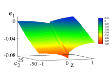
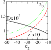
Figure 5: (color online) Left panel: The strain $e_{1}$ as a function of the $z-$coordinate and the $c_{2}$ parameter. Right panel: The depth of the well $D$, and the numerically obtained constants $z_{0}$ and $z^{\star}$ as a function of $c_{2}$. The other Ginzburg-Landau parameters are those for the left and the right material given in Table I.

The values of the Ginzburg-Landau parameters used in the calculations of the strains in Figs. 4 and 5 are given in Table I, calculated from the corresponding elastic coefficients through Eqs. (II). For the left ($L$) material, the second- and third-order constants are those reported for SrTiO₃ Bell1963 ; Beattie1971 , while the second-order constants for the right ($R$) material are those reported recently for LaTiO₃ Liu2011 . The values of the elastic coefficients, whose values are not reported in the literature due to the lack of experimental and theoretical data, are chosen to be reasonable for perovskites (Table I). However,the obtained interfacial effects persists for a wide range of values of the higher-order elastic coefficients. The strain gradient coefficients $d_{1}$ and $d_{2}$ are treated as phenomenological parameters to set the scale of the deformed region. Their values for the left and the right material are chosen to be, respectively, $d_{1}^{L}=d_{2}^{L}=6$ and $d_{1}^{R}=d_{2}^{R}=7$, in units of $10^{-7}~{}N$. For this choise, significant variations in $e_{1}$ and $e_{3}$ occur within $\sim 1$ nm corresponding to $\sim$2-3 TMO layers. The value of $c_{2}$ was taken to be negative for both materials, in accordance with common practices of Ginzburg-Landau theory of phase transitions. In Figs. 4 and 5, where $c_{2}$ and/or $a_{2}$ vary for both materials, a constant ratio between the left and the right value was assumed, calculated from their values given in Table I. The parameter $a_{2}$ is again treated phenomenologically, so that pairs of $a_{2}^{L}$ and $a_{2}^{R}$ with absolute values smaller that those given in Table I (but with the same ratio) have been used. These values are also consistent with the principle $e_{1}<<e_{2},e_{3}$ for all martensitic tranformations.

It has been reported that LaAlO₃ and LaTiO₃ follow the structure of the SrTiO₃ substrate when the latter undergoes a CTT transition Kim2003 ; Wu2011 . The correlation of these structural changes and the electromagnetic properties in these systems may be empirically seen in the observation of an enhancement in the interfacial charge carrier mobility and magnetization below $T_{s}$ Huijben2006 ; Kim2010 ; Christen2008 ; Ariando2011 . In TMO heterostructures undergoing a CTT transition, significant lattice deformation occurs at the interface region due to lattice mismatch, that results in spontaneous strains. Despite the empirical evidence for the effects of interfacial lattice deformation on the electromagnetic properties of TMO heterostructures, the relationship between the strain and the formation of a 2DEG remains largely unexplored. In a Ginzurg-Landau approach that includes charge and/or magnetic degrees of freedom, the dilatational strain $e_{1}$ couples linearly to the charge density Bishop2003 . Then, the results of Fig. 4 reveal that $e_{1}$ serves as an effective potential well which may affect the charge distribution throughout the heterostructure. In particular, the compressed interfacial region may attract and confine electron charges. The localized charges may contribute to the formation of a 2DEG, a prerequisite for interfacial metallicity in TMO heterostructures.

Elastic	Left	Right
Const.	Mater.	Mater.
$C_{11}$	3.172	2.979
$C_{12}$	1.025	1.355
$C_{111}$	-50.0	-47.5
$C_{112}$	-4.0	-3.8
$C_{123}$	-3.0	-2.85
$C_{1111}$	777.5	760.0
$C_{1112}$	270.0	152.0
$C_{1122}$	326.0	342.0
$C_{1123}$	250.0	244.0

GL	Left	Right
Coeff.	Mater.	Mater.
$c_{1}$	1.74	1.89
$c_{2}$	4.29	2.25
$a_{1}$	-3.00	-2.80
$a_{2}$	-31.0	-29.5
$a_{4}$	25.4	24.1
$b_{1}$	48.7	42.9
$b_{2}$	63.3	36.9
$b_{4}$	225	393
$b_{7}$	-35.4	-40.3

Table 1: Second-, third-, and fourth-order elastic coefficients (in units of $10^{11}~{}N/m^{2}$), and Ginzburg-Landau (GL) dimensionless coefficients for the left and the right material used in the calculations.

IV Conclusions

We applied continuum elasticity to investigate theoretically the strain-state of bilayer TMO heterostructures within a Landau theory, and we have obtained simple approximate solutions for the fields $e_{1}$ and $e_{3}$. Interface reconstruction may lead to electronic charge redistribution in the heterostructure, and particularly to electronic charge concentration in the interface region favoring the formation of a 2DEG. The presence of a minimum in the dilatational strain field demonstrates that possibility, linking thus the elastic to the electronic properties of TMOs. Although such a reconstruction is a microscopic phenomenon involving significant changes of atomic arrangements at the interface Chakhalian2007 , it results in macroscopic changes of the unit cells that can be observed experimentally. Those changes can be described, at least qualitatively, by the Ginzburg-Landau theory, and their implications on the electron charge distribution of the bilayer can be inferred from basic physical laws.

Appendix A Nonlinear functions

The nonlinear functions $R_{i}$ ($i=x,y,z$) are given by

$$R_{x}=-a_{4}\left[+e_{2}e_{3}+\frac{1}{2\sqrt{3}}(e_{2}^{2}-e_{3}^{2})\right]$$

$$+\frac{b_{4}}{2}(e_{2}^{2}+e_{3}^{2})\left(+e_{2}+\frac{1}{\sqrt{3}}e_{3}\right)$$

$$+\frac{3a_{1}}{2}e_{1}^{2}+\frac{a_{2}}{2}\left[(e_{2}^{2}+e_{3}^{2})+e_{1}\left(+e_{2}+\frac{1}{\sqrt{3}}e_{3}\right)\right]$$

$$+b_{1}e_{1}^{3}+b_{2}e_{1}(e_{2}^{2}+e_{3}^{2})+\frac{b_{2}}{2}e_{1}^{2}\left(+e_{2}+\frac{1}{\sqrt{3}}e_{3}\right)$$

$$+\frac{b_{7}}{2}\left[e_{3}(e_{3}^{2}-3e_{2}^{2})-3e_{1}e_{2}e_{3}+\frac{\sqrt{3}}{2}e_{1}(e_{3}^{2}-e_{2}^{2})\right]$$ (26)

$$R_{y}=-a_{4}\left[-e_{2}e_{3}+\frac{1}{2\sqrt{3}}(e_{2}^{2}-e_{3}^{2})\right]$$

$$+\frac{b_{4}}{2}(e_{2}^{2}+e_{3}^{2})\left(-e_{2}+\frac{1}{\sqrt{3}}e_{3}\right)$$

$$+\frac{3a_{1}}{2}e_{1}^{2}+\frac{a_{2}}{2}\left[(e_{2}^{2}+e_{3}^{2})+e_{1}\left(-e_{2}+\frac{1}{\sqrt{3}}e_{3}\right)\right]$$

$$+b_{1}e_{1}^{3}+b_{2}e_{1}(e_{2}^{2}+e_{3}^{2})+\frac{b_{2}}{2}e_{1}^{2}\left(-e_{2}+\frac{1}{\sqrt{3}}e_{3}\right)$$

$$+\frac{b_{7}}{2}\left[e_{3}(e_{3}^{2}-3e_{2}^{2})+3e_{1}e_{2}e_{3}+\frac{\sqrt{3}}{2}e_{1}(e_{3}^{2}-e_{2}^{2})\right]$$ (27)

$$R_{z}=-\frac{1}{\sqrt{3}}\left[-a_{4}(e_{2}^{2}-e_{3}^{2})+b_{4}e_{3}(e_{2}^{2}+e_{3}^{2})\right]$$

$$+\frac{3a_{1}}{2}e_{1}^{2}+\frac{a_{2}}{2}\left[(e_{2}^{2}+e_{3}^{2})-\frac{2}{\sqrt{3}}e_{1}e_{3}\right]$$

$$+b_{1}e_{1}^{3}+b_{2}\left[e_{1}(e_{2}^{2}+e_{3}^{2})-\frac{1}{\sqrt{3}}e_{1}^{2}e_{3}\right]$$

$$+\frac{b_{7}}{2}\left[e_{3}(e_{3}^{2}-3e_{2}^{2})-\sqrt{3}e_{1}(e_{3}^{2}-e_{2}^{2})\right]$$ (28)

It can be easily checked that for $e_{2}=0$ we have $R_{x}=R_{y}$.

References

- (1) A. Ohtomo, D. A. Muller, J. L. Grazul, and H. Y. Hwang, Nature 419, 378 (2002).
- (2) A. Ohtomo and H. Y. Hwang, Nature 427, 423 (2004).
- (3) K. Shibuya, T. Ohnishi, M. Kawasaki, H. Koinuma, and M. Lippmaä, Jpn. J. Appl. Phys. 43, L1178 (2004).
- (4) S. Okamoto, A. J. Millis, and N. A. Spaldin, Phys. Rev. Lett. 97, 056802 (2006).
- (5) H. Ishida and A. Liebsch, Phys. Rev. B 77, 115350 (2008).
- (6) F. J. Wong, S.-H. Baek, R. V. Chopdekar, V. V. Mehta, Ho-Won Jang, C.-B. Eom, and Y. Suzuki, Phys. Rev. B 81, 161101(R) (2010).
- (7) E. K. H. Salje, ”Phase Transitions in Ferroelastic and Co-elastic Crystals”, (Cambridge University Press, Cambridge, 1990).
- (8) S. S. A. Seo, W. S. Choi, H. N. Lee, L. Yu, K. W. Kim, C. Bernhard, and T. W. Noh, Phys. Rev. Lett. 99, 266801 (2007).
- (9) J. Biscaras, N. Bergeal, A. Kushwaha, T. Wolf, A. Rastogi, R. C. Budhani, and J. Lesueur, Nat. Comms. 1, 89 (2010).
- (10) J. S. Kim, S. S. A. Seo, M. F. Chisholm, R. K. Kremer, H.-U. Habermeier, B. Keimer, and H. N. Lee, Phys. Rev. B 82, 201407(R) (2010).
- (11) K. H. Kim, D. P. Norton, J. D. Budai, M. F. Chisholm, B. C. Sales, D. K. Christen, and C. Cantoni, Phys. Stat Sol. (a) 200, 346 (2003).
- (12) S. X. Wu, H. Y. Peng, and T. Wu, Appl. Phys. Lett. 98, 093503 (2011).
- (13) K. H. Ahn, T. Lookman, and A. R. Bishop Nature 428, 401 (2004).
- (14) A. R. Bishop, J. Phys.: Conf. Series 108, 012027 (2008).
- (15) P. Maniadis, T. Lookman, and A. R. Bishop, Phys. Rev. B 78, 134304 (2008).
- (16) C. W. Bark, D. A. Felker, Y. Wang, Y. Zhang, H. W. Jang, C. M. Folkman, J. W. Park, S. H. Baek, H. Zhou, D. D. Fong, X. Q. Pan, E. Y. Tsymbal, M. S. Rzchowski, and C. B. Eom, PNAS 108, 4720 (2011).
- (17) J. W. Seo, W. Prellier, P. Padhan, P. Boullay, J.-Y. Kim, H. Lee, C. D. Batista, I. Martin, E. E. M. Chia, T. Wu, B.-G. Cho, and C. Panagopoulos, Phys. Rev. Lett. 105, 167206 (2010).
- (18) Ho Nyung Lee, H. M. Christen, M. F. Chisholm, C. M. Rouleau, and D. H. Lowndes, Nature 433, 395 (2005).
- (19) J. H. Lee, L. Fang, E. Vlahos, X. Ke, Y. W. Jung, L. Fitting-Kourkoutis, J.-W. Kim, P. J. Ryan, T. Heeg, M. Roeckerath, V. Goian, M. Bernhagen, R. Uecker, P. C. Hammel, K. M. Rabe, S. Kamba, J. Schubert, J. W. Freeland, D. A. Muller, C. J. Fennie, P. Schiffer, V. Gopalan, E. Johnston-Halperin, and D. G. Schlom, Nature 466, 954 (2010).
- (20) G. C. Milward, M. J. Calderon, and P. B. Littlewood, Nature 433, 607 (2005).
- (21) J. Chakhalian, J. W. Freeland, G. Cristiani, G. Khaliullin, M. van Veenendaal, and B. Keimer, Science 318, 1114 (2007).
- (22) S. Okamoto and A. J. Millis, Nature 428, 630 (2004).
- (23) A. E. Jacobs, S. H. Curnoe, and R. C. Desai, Phys. Rev. B 68, 224104 (2003).
- (24) K. Ø. Rasmussen, T. Lookman, A. Saxena, A. R. Bishop, R. C. Albers, and S. R. Shenoy, Phys. Rev. Lett. 87, 055704 (2001).
- (25) A. Kosogor, V. A. L’vov, O. Söderberg, S.-P. Hannula, Acta Mater. 59, 3593 (2011).
- (26) V. A. Chernenko and V. A. L’Vov, Phil. Mag. A 73, 999 (1996).
- (27) G. R. Barsch and J. A. Krumhansl, Phys. Rev. Lett. 53, 1069 (1984).
- (28) E. V. Gomonaj and V. A. L’Vov, Phase Transit. 47, 9 (1994);
- (29) E. V. Gomonaj and V. A. L’Vov, Phase Transit. 56, 43 (1996).
- (30) J. K. Liakos and G. A. Saunders, Philos. Mag. A 46, 217 (1982).
- (31) R. O. Bell and G. Rupprecht, Phys. Rev. 129, 90 (1963).
- (32) A. G. Beattie and G. A. Samara, J. Appl. Phys. 42, 2376 (1971).
- (33) V. A. Chernenko, M. Kohl, V. A. L’vov, V. M. Kniazkyi, M. Ohtsuka, and O. Kraft, Mater. Trans. 47, 619 (2006).
- (34) V.A. Chernenko, M. Kohl, M. Ohtsuka, T. Takagi, V. A. L’vov, V. M. Kniazky, Mater. Sci. Eng. A 438-440, 944 (2006).
- (35) A. T. J. Helvoort, Ø. Dahl, B. G. Soleim, R. Holmestad, and T. Tybell, Appl. Phys. Lett. 86, 092907 (2005).
- (36) W. L. Ling, J. de la Figuera, N. C. Bartelt, R. Q. Hwang, A. K. Schmid, G. E. Thayer, and J. C. Hamilton, Phys. Rev. Lett. 92, 116102 (2004).
- (37) C.-M. Liu, N.-N. Ge, and G.-F. Li, Physica B 406, 1926 (2011).
- (38) M. Huijben, G. Rijnders, D. H. A. Blank, S. Bals, S. Van Aert, Jo Verbeeck, G. Van Tendeloo, A. Brinkman, and H. Hilgenkamp, Nature Mater. 5, 556 (2006).
- (39) H. M. Christen, D. H. Kim, and C. M. Rouleau, Appl. Phys. A 93, 807 (2008).
- (40) Ariando, X. Wang, G. Baskaran, Z. Q. Liu, J. Huijben, J. B. Yi, A. Annadi, A. Roy Barman, A. Rusydi, S. Dhar, Y. P. Feng, J. Ding, H. Hilgenkamp, and T. Venkatesan, Nat. Comms. 2, 188 (2011).
- (41) A. R. Bishop, T. Lookman, A. Saxena, and S. R. Shenoy, Europhys. Lett. 63, 289 (2003).