Domain Adaptation:
Overfitting and Small Sample Statistics

Abstract

We study the prevalent problem when a test distribution differs from the training distribution. We consider a setting where our training set consists of a small number of sample domains, but where we have many samples in each domain. Our goal is to generalize to a new domain. For example, we may want to learn a similarity function using only certain classes of objects, but we desire that this similarity function be applicable to object classes not present in our training sample (e.g. we might seek to learn that “dogs are similar to dogs” even though images of dogs were absent from our training set). Our theoretical analysis shows that we can select many more features than domains while avoiding overfitting by utilizing data-dependent variance properties. We present a greedy feature selection algorithm based on using $T$-statistics. Our experiments validate this theory showing that our $T$-statistic based greedy feature selection is more robust at avoiding overfitting than the classical greedy procedure.

1 Introduction

The generalization ability of most modern machine learning algorithms are predicated on the assumption that the distribution over training examples (roughly) matches the distribution over the test data. There is growing literature studying settings where this implicit assumption fails to hold — often referred to as domain adaptation or transfer learning. This problem is central in fields such as speech recognition [19], computational biology [20], natural language processing [5, 8, 12], and web search [6, 11].

We examine how severe this problem can be, even on one of the most conventional benchmark datasets, the MNIST digits dataset. Here, state-of-the-art algorithms reliably obtain classification error rates below $1\%$, when recognizing one digit vs. the other digits. Consider a natural modification of this setting where we train a model to recognize the digit “$2$” vs. the other even digits. If we learn to recognize a “$2$” accurately (vs. only even digits), then we may hope that our classifier will robustly recognize a “$2$” against new odd digits. Unfortunately, this is far from being true: a logistic regression algorithm, trained on this dataset and achieving a (true) test error rate of about $0.5\%$ (against even digits), jumps to $35\%$ error rate when tested vs. odd digits, a startling $7000\%$ increase in error. While the present work uses deep belief network features [13], trained on unlabeled data, this situation is generic across many other common training methods we have tried: SVMs with various kernels and logistic/linear regression with various feature choices (where error rates increase from hundreds to thousands of percent depending on the details of the experiment).

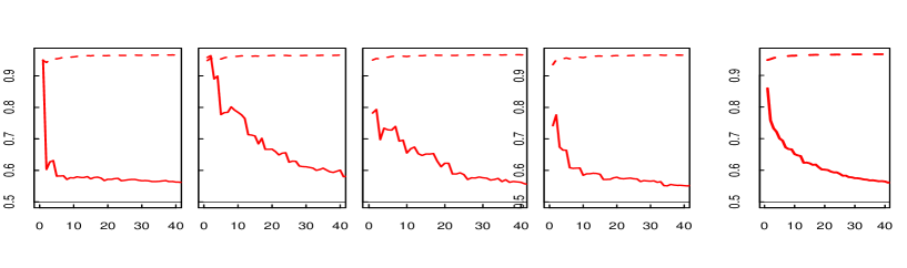
Figure 1: Area under ROC (AUROC) (y-axis) for predicting digit ’2’ using the greedy algorithm. The x-axis shows the order of variables were picked out of 2000 total variables. The top dashed line shows generalization or ’test’ performance on the source domain. The transfer to a new domain is shown below it as the solid line. The last figure on the right shows the average of all the ROC curves. The horizontal line is at “chance.”

We elucidate this overfitting issue by examining how various “area under the ROC curves” change as we greedily add more features. Here, we train our model to recognize the digit “$2$” vs. eight other digits, and test recognition of a “$2$” vs. the remaining digit (with balanced distributions where a “$2$” appears half the time in both the training and test distributions). The first four plots in Figure 1 show the test performance using the area under the ROC metric on the training distribution (the dashed red curve) and on the test distribution (the solid red curve) vs. the number of features we have greedily added. Note two striking effects: 1) how rapidly the test performance plummets; 2) more troubling, how quickly the test performance for the training and test distributions diverge. In particular, note that the true generalization performance on the source training distribution is not at all reflective of the true generalization performance on the target test distribution, even after adding just a few features: a classic example of overfitting. The final plot shows the average of the training and test performance, averaged over which digit is held out, and cycling through digits.

Overfitting is to be expected, because this experiment violates the learning theoretic preconditions for successful generalization. Furthermore, for this particular experiment, we could argue that a generative approach is more robust: if we have a model for generating a “$2$”, then it should be good for recognition in diverse settings. While the generative framework is promising, particularly for generating predictive features, it is often difficult to specify good generative models.

In this work, we assume a distribution over domains, and that our training sample consists of a small number of sample domains independently drawn from the distribution over domains and where we have access to many samples in each domain. The goal in our setting is to perform well on new domains sampled from this distribution. For example, in the previous experiments, we can consider that we have eight sample (known) domains in our training set, where domains are of the form “2 vs. 0”, “2 vs. 1”, “2 vs. 3”, etc. This is much like the standard supervised learning model, except that sampled “points” are now “domains”. The challenge is that we desire to avoid overfitting with an extremely small number of domains, or few “samples”, compared to standard supervised learning paradigms, that assume hundreds to millions of samples.

The problem of domain adaptation is more general than this particular formulation, where our focus is on how to do well on a new random domain. There are numerous different aspects of the domain adaptation problem that have been studied. For example, assumptions considered are: when the classes are “imbalanced” (e.g. when $\Pr[Y|D]$ could vary with the domain $D$); “covariate shift” [4] where $\Pr[X|D]$ varies with the domain $D$, while $\Pr[Y|X,D]$ is not a function of the domain; under a change of representation, the joint distributions of $\Pr[(X,Y)|D]$ is more similar [5, 21, 12, 14, 16]; settings where one desires mixtures of predictors which adapt to each domain [9]. A detailed discussion of these models is beyond the scope of this paper (see [17] for a more comprehensive review.). There is also a growing body of theoretical work on this problem, including [15, 2, 7, 1] that concentrates on either characterizing the degradation that can occur due to distributional shift (e.g.  [2]) or robustly training using biased sampling, such as the sample selection bias work of  [7].

Our work differs in that we assume a distribution over domains, and our focus is on generalization on new domains. One interesting application of this work is on learning similarity functions. For example, we may desire to learn a similarity function for objects, where objects of the same label have high similarity, in manner so as to be able to utilize this similarity function to recognize new objects, not present in our training set; a problem known as “zero-shot” learning.

Our Contributions: Our analysis focuses on the issue of overfitting, and we borrow the idea from small sample statistics that a certain empirical variance should be utilized when deciding whether or not an effect is significant, namely, that an added feature will decrease our error. We do this using $T$-statistics. The key idea is that we can estimate the weight of each feature on each training domain separately. Indeed, if this weight varies wildly over the training source domains, then even though this feature may be useful on all our source domains, its potential for generalization to new domains may be poor. We show that our data-dependent version of feature selection robustly enjoys the usual feature selection properties, i.e. we can select many more features than domains, particularly if certain data-dependent variances are low, under relatively weak assumptions.

The contributions of this work are as follows:

• Using small sample statistics, namely that of $T$-tests, we provide a more robust procedure to add features, which takes into account data-dependent properties.

• Using the theory of large deviations for self-normalized sums, we show that we can robustly add many more feature than domains (exponentially more), utilizing certain empirical variances.

• We empirically demonstrate that we control for overfitting using an alternative greedy procedure for feature addition, based on the $T$-statistic. In particular, we show that these ideas can be utilized towards the theory of “zero-shot learning”.

2 Setting

A key idea in our setting is that we consider a distribution over domains, which we denote by $\Pr[D]$ (it is possible that there may be an infinite number of domains). Conditioned on a domain $D=d$, the distribution over input/output pairs is $\Pr[(X,Y)|D=d]$, where our inputs are $X\in{\mathbb{R}}^{p}$. As is standard, these inputs could represent a high dimensional feature space. The goal is to find a weight vector which minimizes the squared error, averaged over both instances and over the domains. More precisely, the error we want to minimize is:

$${\cal L}(w)={\mathbb{E}}_{D}{\mathbb{E}}_{X,Y}[(Y-w\cdot X)^{2}|D]$$

where the inner and outer expectations are over $(X,Y)$ and $D$, respectively.

Our training set consists of a set of $n$ known domains $\{d_{1},d_{2},\ldots d_{n}\}$, where each domain is sampled independently. In practice, while $n$ is small, we often have a large number of samples in each domain, so that the second order statistics can be estimated accurately on each training domain. As a natural abstraction, we assume that for each domain $d$ in our training set, we have knowledge of both ${\mathbb{E}}[XY|D=d]$ and ${\mathbb{E}}[XX^{\top}|D=d]$.

For our theoretical analysis, we also assume the joint input covariance matrix ${\mathbb{E}}[XX^{\top}]$ is known, as it can be estimated accurately with unlabeled data. This permits a cleaner exposition in terms of unbiased estimation, although this distinction is relatively minor in practice.

3 Feature Selection and Small Sample Statistics

Our goal is to avoid overfitting while adding features: we desire confidence that our added feature actually improves the error on new domains. The naive greedy method is to add features which maximally decreases our training set error, which, as we have shown in the Introduction, can perform remarkably poorly. Instead, we provide a theory which more sharply characterizes when adding a feature actually improves our performance.

3.1 Adding a Single Feature

We first investigate the question of whether or not a single feature improves the null prediction of always saying $0$. It is natural to base our theory using unbiased estimates, as we often have the most robust statistical tests for these estimates.

Consider a feature $X_{i}$, which is normalized so that ${\mathbb{E}}[X_{i}^{2}]=1$. The optimal weight on this feature is $w^{*}_{i}={\mathbb{E}}[X_{i}Y]$. Furthermore, any weight $w_{i}$ on $X_{i}$ has regret:

$${\cal L}(w_{i})-{\cal L}(w^{*}_{i})=(w_{i}-{\mathbb{E}}[X_{i}Y])^{2}$$

Hence, with respect to adding just one feature, our task is to find a feature $X_{i}$ and weight vector $w_{i}$ such that we have confidence that $w_{i}$ is closer to ${\mathbb{E}}[X_{i}Y]$ than $0$ is (as weight $0$ corresponds to the null prediction). The natural unbiased estimate for $w^{*}_{i}$ is simply:

$${\widehat{\mu}}_{i}=\frac{1}{n}\sum_{k=1}^{n}{\mathbb{E}}[X_{i}Y|d_{k}]$$

The Central Limit Theorem implies that ${\widehat{\mu}}_{i}$ should be close to ${\mathbb{E}}[X_{i}Y]$ on the order of $O(\frac{\sigma(X_{i}Y)}{\sqrt{n}})$, where $\sigma(X_{i}Y)$ is the standard deviation. A key idea in small sample statistics is to take into account the empirical variance. Here, when determining if $X_{i}$ is useful, we seek to consider the (unbiased) variance estimate:

$${\widehat{\sigma}}_{i}^{2}=\frac{1}{n-1}\sum_{k=1}^{n}({\mathbb{E}}[X_{i}Y|d_{k}]-{\widehat{\mu}}_{i})^{2}$$

and the issue is how to utilize this estimate rather than the true variance.

In our domain adaptation setting, it may be the case that this covariance for certain “robust” features ${\mathbb{E}}[X_{i}Y]$ is more consistently correlated with the target — it is these features that we seek to add. By contrast, “large” sample analysis typically involves only using an upper bound on the standard deviation $\sigma(X_{i}Y)$, along with tail bounds such as the Bernstein bound [3], to get estimates on the deviation between ${\widehat{\mu}}_{i}$ and its mean. However, crucially, as $\sigma(X_{i}Y)$ could vary greatly with our feature $X_{i}$, we desire a sharper estimate which takes into account the empirical variance, ${\widehat{\sigma}}_{i}^{2}$.

If ${\widehat{\mu}}_{i}$ followed a normal distribution, then this question reduces to a Student’s $T$-test. Here, the $T$ statistic is:

$$T_{i}=\frac{\hat{\mu}_{i}}{\hat{\sigma}_{i}/\sqrt{n}}$$

While we do not expect the ${\widehat{\mu}}_{i}$ to actually follow a normal distribution, there is a rather large literature showing that the $T$-test is robust (see for example  [10]). We now demonstrate this point under a milder assumption, that $\hat{\mu}_{i}$ is symmetric (where the source of randomness is from a random domain). Equivalently, this is an assumption that the covariances ${\mathbb{E}}[X_{i}Y|d]$ are symmetric about their mean (i.e. both ${\mathbb{E}}[X_{i}Y|d]-{\mathbb{E}}[X_{i}Y]$ and $-({\mathbb{E}}[X_{i}Y|d]-{\mathbb{E}}[X_{i}Y])$ have the same distribution, where $d$ is the source of randomness). The following theorem assumes no moment conditions on $X_{i}$ or $Y$ (not even upper bounds). It shows that we can accurately test an exponential number of features with high confidence. This bound has similar behavior to the $T$-distribution (for fixed $n$) as we scale the number of features.

Theorem 1.

Assume the random vector ${\mathbb{E}}[XY|d]-{\mathbb{E}}[XY]$ is symmetric (where $d$ is random). Let $\delta>0$. Suppose ${\cal F}$ is a set of features whose size satisfies $|{\cal F}|\leq\frac{\delta}{2}e^{\frac{n}{8}}$ (e.g. it is of size at most exponential in $n$). Then for all $X_{i}$ in ${\cal F}$, we have with probability greater than $1-\delta$:

$$|\hat{\mu}_{i}-{\mathbb{E}}[X_{i}Y]|\leq\frac{{\widehat{\sigma}}_{i}}{\sqrt{n}}\ \sqrt{4\log\frac{2|{\cal F}|}{\delta}}$$

where no moment bounds on $X$ and $Y$ are assumed, aside from existence of ${\mathbb{E}}[XY|d]$ and ${\mathbb{E}}[XY]$.

The proof of this theorem is in the appendix. The key is that this theorem shows that the empirical variance can be taken into account when searching through a large feature set. In fact, asymptotically, as implied by the Central Limit Theorem, the only improvement possible is that the constant of $4$ would become a $2$.

The proof (provided in the Appendix) of this bound is significantly more subtle than the standard “Bernstein”-like bounds, since the $T$-statistic has much “thicker” tails. Our proof is based on the following bound for “self-normalized” sums, which, to our knowledge, has not been utilized in the machine learning literature.

Theorem 2.

(See Theorem 2.15 in  [10]) Assume $Z_{1},\ldots Z_{n}$ are independent, mean $0$, symmetric random variables. For all $t>0$, the following bound on the self-normalized sum holds:

$$\Pr\left[\ \frac{({\sum_{i=1}^{n}}Z_{i})^{2}}{{\sum_{i=1}^{n}}Z_{i}^{2}}>t\ \right]\leq\exp\left(-\frac{t}{2}\right)$$

where no moment bounds on $Z_{i}$ are assumed, aside from its mean existing.

For completeness, we add the proof of this theorem in appendix. It is based on a simple symmetrization argument along with Hoeffding’s tail inequality. Note that the above bound is not quite a large deviation bound for a $T$-statistic, as the denominator uses ${\sum_{i=1}^{n}}Z_{i}^{2}$, while a $T$-statistic would have a term of the form ${\sum_{i=1}^{n}}(Z_{i}-\hat{Z})^{2}$, where $\hat{Z}$ is the empirical estimate of the mean, ${\sum_{i=1}^{n}}Z_{i}/n$. This subtlety leads to the condition in Theorem 1 that the size of ${\cal F}$ is at most exponential in $n$.

3.2 Subset Selection

Merely searching for the lowest error solution over all subsets of, say, size $q$ is prone to overfitting. Instead, we seek to take into account the empirical variance when searching over subsets of features. We now provide a data-dependent bound showing that the empirical variance can be utilized for a much sharper bound. In the next subsection, we discuss a greedy method for this search.

Given some set of features ${\cal S}$ of size $q$, let ${\widetilde{X}}_{1}\ldots{\widetilde{X}}_{q}$ be an orthonormal basis for this subspace (e.g. ${\mathbb{E}}[{\widetilde{X}}_{i}{\widetilde{X}}_{j}]$ is $0$ if $i\neq j$ and $1$ if $i=j$. Note that we can put ${\cal S}$ into this basis as we have assumed knowledge of ${\mathbb{E}}[XX^{\top}]$). The best weight vector for this subspace is again the covariance $[\mu_{S}]_{i}={\mathbb{E}}[{\widetilde{X}}_{i}Y]$. Define the (unbiased) empirical means and variances as follows:

$$[{\widehat{\mu}}_{S}]_{i} = \frac{1}{n}\sum_{k=1}^{n}{\mathbb{E}}[{\widetilde{X}}_{i}Y|d_{k}],$$

$$\textrm{{ }}[{\widehat{\sigma}}_{S}]_{i}^{2} = \frac{1}{n-1}\sum_{k=1}^{n}({\mathbb{E}}[{\widetilde{X}}_{i}Y|d_{k}]-[{\widehat{\mu}}_{S}]_{i})^{2}$$

We take ${\widehat{\mu}}_{S}$ as the estimate of the weight vector on this subspace. We now provide our data dependent generalization bound, in terms of an appropriate empirical variance. In particular, we are interested in a generalization bound for all subsets of size $q$ out of a feature set of size $p$.

Corollary 3.

Assume the random vector ${\mathbb{E}}[XY|d]-{\mathbb{E}}[XY]$ is symmetric. Let $\delta>0$. Assume that our set of features ${\cal F}$ is of size $p$, and that $qp^{q}\leq\frac{\delta}{2}e^{\frac{n}{8}}$. For all subsets ${\cal S}\subset{\cal F}$ of size $q$, we have:

$$L({\widehat{\mu}}_{S})-L(\mu_{S})\leq\left(\sum_{i\in{\cal S}}[{\widehat{\sigma}}_{S}]_{i}^{2}\right)\frac{8q\log p+\log(2/\delta)}{n}\vspace{-0.1in}$$

This bound is analogous to the usual bounds for regression where instead of the sum empirical variance, we have the true variance (which is usually assumed to be constant in idealized Gaussian noise regression model). Crucially, the bound shows that we can robustly utilize the empirical variance when doing our estimation. The implications of this are that we can design a much sharper procedure for testing if a feature improves performance.

3.3 Practice: The T-Greedy Algorithm

In practice, the natural methodology is to “greedily” choose a feature instead of searching all subsets, which usually consists of finding the feature which decreases the error the most. Instead, we introduce the $T$-greedy algorithm, a “stagewise” procedure for adding the feature which has the highest $T$-statistic (e.g. the goal is to add a feature in which we have the most confidence that the true error will be improved).

There are a variety of greedy regression procedures, such as “stepwise”,“stagewise”, etc. We now present a stagewise variant by considering covariances with our residual error $(Y-w\cdot X)$. Suppose that our current weight vector is $w$ (on our current set of features). For each feature $X_{i}$, we compute the empirical mean and variance:

$${\widehat{\mu}}_{i} = \frac{1}{n}\sum_{k=1}^{n}{\mathbb{E}}[X_{i}(Y-w\cdot X)|d_{k}],$$

$${\widehat{\sigma}}_{i}^{2} = \frac{1}{n-1}\sum_{k=1}^{n}({\mathbb{E}}[X_{i}(Y-w\cdot X)|d_{k}]-{\widehat{\mu}}_{i})^{2}$$

Note that with a finite number samples in each domain, we would simply use the empirical estimates instead. Now we just add the feature with the highest $T$-statistic, e.g. add the feature:

$$i^{\star}={\rm arg}\max_{i}T_{i}$$

where $T_{i}=\frac{\hat{\mu}_{i}}{\hat{\sigma}_{i}/\sqrt{n}}$. Now our update to the weight on this feature is simply:

$$w_{i^{\star}}\leftarrow w_{i^{\star}}+\frac{{\widehat{\mu}}_{i}}{\hat{\mathbb{E}}[X_{i}^{2}]},\quad\hat{\mathbb{E}}[X_{i}^{2}]=\frac{1}{n}\sum_{k=1}^{n}{\mathbb{E}}[X_{i}^{2}|d_{k}]$$

Observe that this is actually a biased estimate of the optimal weight on this added feature. Technically, our theory is only applicable to using unbiased estimates, where we would have ${\mathbb{E}}[X_{i}^{2}]$ in the denominator. This is a minor distinction in practice, and with unlabeled data we could essentially run the unbiased version. We should point out that stepwise variants are also possible.

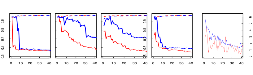
Figure 2: Area under ROC (AUROC) (y-axis) for predicting digit ’2’ for both the greedy algorithm (shown in red) and for our $T$-greedy algorithm (shown in blue), as we add more features (x-axis). Since we choose features based on T-statistics (see last graph), our T-statistics is generally higher than that of the greedy algorithm.

4 Experimental Results

We now present results on the MNIST and CIFAR image datasets. The MNIST digit dataset contains 60,000 training and 10,000 test images of ten handwritten digits (0 to 9), with 28$\times$28 pixels. In all experiments, we use 10,000 digits (1,000 per class) for training and 10,000 digits for testing. Instead of using raw pixel values, each image was represented by 2000 real-valued features, that were extracted using a deep belief network [13].

We also present results on the more challenging CIFAR image dataset [18], that contains images of 10 object categories, including airplane, car, bird, cat, dog, deer, truck, deer, frog, and horse. As with the MNIST dataset, we use 10,000 images (1,000 per class) for training and 10,000 images for testing. Each image was also represented by 2000 real-valued features, that were extracted using a deep belief network [18]. We note that extreme variability in scale, viewpoint, illumination, and cluttered background, makes object recognition task for this dataset difficult.

In all experiments, we report the area under ROC (AUROC) metric of two different algorithms, that we refer to as the greedy and our proposed T-greedy algorithm. The greedy algorithm chooses the next feature which decreases the squared loss the most on the training set. The T-greedy algorithm, on the other hand, chooses a feature with the largest T-statistic. For both methods, we report both generalization error on our training or ’source’ domains as well as generalization error on test or ’target’ domains. We do not focus on the issue of stopping but rather on robustness. There are a variety of methods for stopping which we mention in the Discussion section.

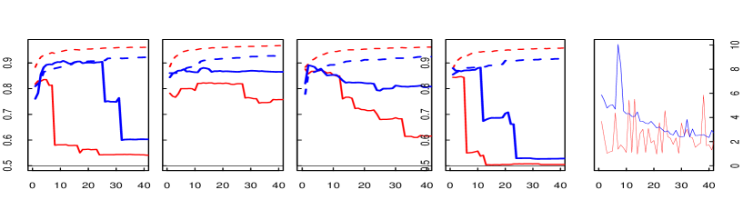
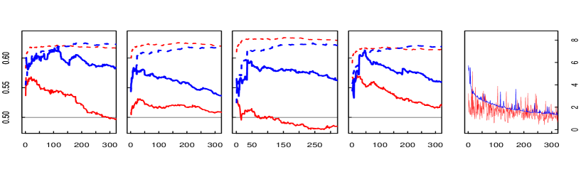
Figure 3: Area under ROC (AUROC) (y-axis) for learning similarity function for both the greedy algorithm (shown in red) and for our $T$-greedy algorithm (shown in blue), as we add more features (x-axis). Since we choose features based on T-statistics, our T-statistics are generally higher than that of the greedy algorithm.

4.1 MNIST (2 vs. other)

In our first experiment, shown as the leftmost plot in Fig. 2, we tested the ability of the proposed algorithm to generalize to a new target domain: recognizing the digit ’2’ vs. the new, previously unseen digit ’9’. To this end, we created eight source domains: {’2’ vs. ’0’},…, {’2’ vs. ’8’}, where each domain contained a balanced set of 2000 labeled training examples. Our new target domain (as the test set) {’2’ vs. ’9’} also contained a balanced set of 2000 examples.

Fig. 2, the leftmost plot, displays an evolution of the area under ROC (AUROC) metric for both greedy (red curves) and $T$-greedy (blue curves) algorithms. Note that an area of 0.5 corresponds to a random classifier, shown on the graph as a horizontal line. The dashed curves correspond to generalization or ’test’ performance on the source domains, whereas the solid curves display performance on the target domain. Observe that after adding a few features, test performance of the greedy algorithm on the new target domain (red solid curve) rapidly decreases. Test error on the source domains, however, keeps improving, clearly demonstrating that no overfitting on the source domains is occurring. Hence, for the greedy algorithm, the true error on the source and target domains rapidly diverge.

This is in sharp contrast to the performance of the $T$-greedy algorithm. Even though performance of the $T$-greedy algorithm on the source domains (blue dashed curve) is slightly worse (as expected as it is not as aggressively striving for source error minimization), the true AUROC on the source and target domains diverges less rapidly — in particular, these curves start close together. Fig. 2 further shows results for different source/target splits. We consistently observe that as we add few features, the $T$-greedy algorithm overfits much less on the target domain. This consistency is also seen in left most plot of Fig. 4, that displays results averaged over all splits of the source and target domains.

The rightmost plot of Fig. 2 also shows the $T$-statistic of the added feature to the model of both algorithms. We only show one such figure since they all look similar.

We formulate the similarity learning problem in our regression setting as follows. Given two feature vectors corresponding to two images $\phi(X^{1})$ and $\phi(X^{2})$, we consider a linear regression function:

$$y=\textrm{sgn}(\sum_{i}w_{i}\phi_{i}(X^{1})\phi_{i}(X^{2})),$$

where we set $y=1$ if two images have the same label (positive example), and $y=-1$ if two images have different labels (negative example).

Fig. 3, top row, displays results on learning a similarity function for MNIST digits. In particular, consider learning a similarity function on all the digits, but with digit ’9’ excluded. Similar to the previous experiment, we constructed nine source domains (corresponding to digits 0 through 8). Each domain contained 1000 positive and 1000 negative examples, where negative examples were randomly sampled from the remaining digits in the source domain. Our target domain contained 1000 positive examples of newly observed images of ’9’ and 1000 negative examples, randomly sampled from images of 0-to-8.

4.2 Learning similarity function

We now consider a more demanding task of learning a similarity function between two images. A good similarity function can provide insight into how high-dimensional data is organized and can significantly improve the performance of many machine learning algorithms that are based on computing similarity metric. Our goal is to learn a similarity function that can not only work well for objects that are part of the training set, but also works well for new objects that we may have never seen before: a widely studied problem known as a “zero-shot” learning.

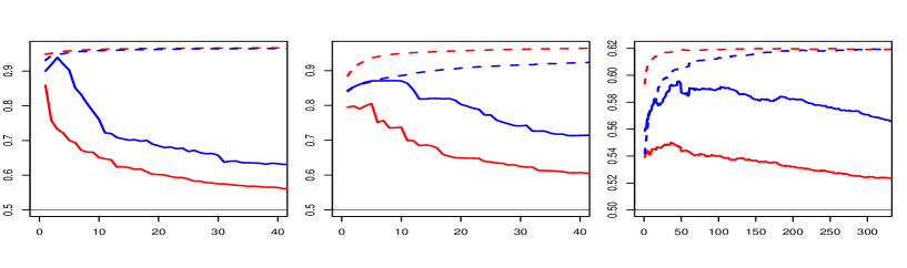
Figure 4: Area under ROC averaged over all splits of source/target domains for predicting digit 2 (left), learning similarity function for MNIST digits (middle) and CIFAR images (right).

Fig. 3, top leftmost plot, shows that the generalization error of the greedy algorithm on the source and target domains rapidly diverge. The $T$-greedy, on the other hand, is able to select up to 25 reliable features that help us generalize well to the new target domain. Fig. 3 further displays performance results when generalizing a similarity function to different target domains. Again, the rightmost plot shows the value of the added $T$-statistic for one of these plots.

Finally, we experimented with learning a similarity function for more challenging image CIFAR dataset. Similar to the results on the MNIST dataset, Fig. 3, bottom row, shows that the $T$-greedy algorithm is able to consistently pick up to 50 robust features that are useful for transfer to a new domain (note the difference in scale on the $x$-axis, which now goes to 300 features). The greedy algorithm, however, barely improves upon making random predictions.

We have focused attention on the individual domains to help drive home how variable each domain is from the others. But, it is sometimes hard to see the signal amongst all this noise, so we also provide averaged versions of the AUROC curves (Fig. 4). The $T$-greedy algorithm is able to pick up many more robust features and overfits far less on the target domain (difference in blue-dashed and blue-solid curves). The greedy algorithm’s test error diverges after adding only a handful of features. Almost immediately we see a big gap in the error on the source and target domains (difference in red-dashed and red-solid curves).

5 Discussion

All experiments demonstrate that the $T$-greedy algorithm has better correspondence between training AUROC and testing AUROC. The curves start out with the training and the testing AUROC curves with about the same value. This is particularly striking in the averaged curves, shown in Fig. 4. So by looking only at the training curves one can get a good estimate of the generalization performance. As expected, eventually overfitting occurs, since the training AUROC continues to improve whereas the testing AUROC decreases. However, even then it is possible to get a handle on using our method (e.g. when to stop). One option is to simply keep yet another domain held out for cross-validation and cycle through. Alternatively, we can use properties of the T-statistic to get a handle on when to stop (e.g. when the $T$-statistics is behaving like chance). Here, Bonferoni can also be used as a heuristic to decide how many variables to use. Again, this is made easier by the fact that the curves are close.

We also observe that the variability between domains is much greater than the variability within any given domain (Figs. 2, 3, and 4 all show this variability). Classical statistics assumes that each error is independent (if just merged across all the domains), but we see from plots that each domain behaves idiosyncratically. Sometimes they overfit after a few variables, sometimes they continue to improve. This means that using more observations from the domains we have already studied is not informative of how we will extrapolate to new domains. Such small sample sizes were the original motivation for Gosset to come up with his Student’s T-statistic. Note that we do not have many degrees of freedom but we can still obtain as much information out of the data we have. What we see from our analysis and experiments is that this information can still be substantial.

Acknowledgments

RS is supported by NSERC, and NTT Communication Sciences Laboratory.

Appendix A Appendix

First, let us prove Theorem 2 (also, see Theorem 2.15 in  [10]).

Proof.

(of Theorem 2). Let ${\epsilon}_{i}$ be Rademacher random variables (e.g. independent random variables which take values uniformly in $\{-1,1\}$). Since each $Z_{i}$ is symmetric, we have that the distribution of $Z_{i}$ is identical to the distribution of ${\epsilon}_{i}Z_{i}$. Hence, we have that:

$$\Pr\left[\ \frac{({\sum_{i=1}^{n}}Z_{i})^{2}}{{\sum_{i=1}^{n}}Z_{i}^{2}}>t\ \right]=\Pr\left[\ \frac{({\sum_{i=1}^{n}}{\epsilon}_{i}Z_{i})^{2}}{{\sum_{i=1}^{n}}Z_{i}^{2}}>t\ \right]$$

Now we bound this latter quantity for every realization of $Z_{i}$. Consider a fixed set of values $z_{1},\ldots z_{n}$ (some realization of $Z_{1},\ldots Z_{n}$). For these fixed values, let us now bound the probability:

$$\Pr\left[\ \frac{({\sum_{i=1}^{n}}{\epsilon}_{i}z_{i})^{2}}{{\sum_{i=1}^{n}}z_{i}^{2}}>t\ \right]\kern-6.0pt = \kern-6.0pt\Pr\left[\ \left({\sum_{i=1}^{n}}{\epsilon}_{i}z_{i}\right)^{2}>t{\sum_{i=1}^{n}}z_{i}^{2}\ \right]$$

$$= \kern-6.0pt\Pr\left[\ \left|{\sum_{i=1}^{n}}{\epsilon}_{i}z_{i}\right|>\sqrt{t{\sum_{i=1}^{n}}z_{i}^{2}}\ \right]$$

$$\leq \kern-6.0pt2\exp\left(-\frac{t{\sum_{i=1}^{n}}z_{i}^{2}}{2{\sum_{i=1}^{n}}z_{i}^{2}}\right)$$

$$= \kern-6.0pt2\exp(-t/2)$$

where the second to last step is by Hoeffding’s inequality (where the only randomness is due to the ${\epsilon}_{i}$). To see this, note that we are adding the independent variables ${\epsilon}_{i}z_{i}$ which are mean $0$ and bounded in magnitude by $z_{i}$. ∎

Now we prove Theorem 1.

Proof.

(of Theorem 1) For symmetric, mean $0$, independent $Z_{i}$, define:

$${\widehat{\mu}}=\frac{1}{n}{\sum_{i=1}^{n}}Z_{i},\quad{\widehat{\sigma}}^{2}=\frac{1}{n-1}{\sum_{i=1}^{n}}(Z_{i}-{\widehat{\mu}})^{2}$$

The $T$-statistic is then defined as:

$$T=\frac{{\widehat{\mu}}}{{\widehat{\sigma}}/\sqrt{n}}$$

Define the related quantity:

$$\widetilde{T}=\frac{{\widehat{\mu}}}{\left(\frac{1}{n}{\sum_{i=1}^{n}}Z_{i}^{2}\right)^{1/2}/\sqrt{n}}$$

and note that:

$$\frac{({\sum_{i=1}^{n}}Z_{i})^{2}}{{\sum_{i=1}^{n}}Z_{i}^{2}}=\widetilde{T}^{2}$$

Also, one can show that $\widetilde{T}^{2}=\frac{n}{n-1}\frac{T^{2}}{1+\frac{T^{2}}{n-1}}$. Hence, using the bound on self-normalized sums,

$$\Pr[T^{2}\geq t^{2}] = \Pr\left[\widetilde{T}^{2}\geq\frac{n}{n-1}\frac{t^{2}}{1+\frac{t^{2}}{n-1}}\right]$$

$$\leq 2\exp\left(-\frac{1}{2}\frac{n}{n-1}\frac{t^{2}}{1+\frac{t^{2}}{n-1}}\right)$$

$$\leq 2\exp\left(-\frac{1}{2}\frac{t^{2}}{1+\frac{t^{2}}{n-1}}\right)$$

Now let us choose $t=\sqrt{4\log\frac{2|{\cal F}|}{\delta}}$. By assumption on the size of ${\cal F}$, we have that $t^{2}\leq n/2$, and so $\frac{t^{2}}{n-1}\leq\frac{n}{2(n-1)}\leq 1$ (since $n\geq 2$). Hence,

$$Pr\left[T^{2}\geq 4\log\frac{2|{\cal F}|}{\delta}\right]\leq 2\exp\left(-\frac{1}{2}\frac{t^{2}}{2}\right)=\frac{\delta}{|{\cal F}|}$$

Our result now follows by the union bound (over all $|{\cal F}|$ features). ∎

Our corollary now follows:

Proof.

(of Corollary 3) For any subset, the regret is:

$$\sum_{i\in{\cal S}}({\widehat{\mu}}_{i}-{\mathbb{E}}[\widetilde{X}_{i}Y])^{2}$$

Now note that there are no more than $p^{q}$ possible subsets. Also, each subset comes with its own basis. So let us demand confidence on all $qp^{q}$ possible basis elements. So we use Theorem 1 with a set of size $qp^{q}$ features (note that the $\log$ of the size of this set is bounded by $2q\log p$). Our theorem now follows by summing over the errors. ∎

References

- [1] J. Baxter. A model of inductive bias learning. Journal of Artificial Intelligence Research, 12:149–226, 2000.
- [2] S. Ben-David, J. Blitzer, K. Crammer, and F. Pereira. Analysis of representations for domain adaptation. In NIPS, 2007.
- [3] S. Bernstein. The Theory of Probabilities. Gastehizdat Publishing House, Moscow, 1946.
- [4] Steffen Bickel, Michael Brückner, and Tobias Scheffer. Discriminative learning for differing training and test distributions. In In ICML, pages 81–88. ACM Press, 2007.
- [5] J. Blitzer, R. McDonald, and F. Pereira. Domain adaptation with structural correspondence learning. In EMNLP, 2006.
- [6] K. Chen, R. Liu, C.K. Wong, G. Sun, L. Heck, and B. Tseng. Trada: tree based ranking function adaptation. In CIKM, 2008.
- [7] C. Cortes, M. Mohri, M. Riley, and A. Rostamizadeh. Sample selection bias correction theory. In ALT, 2008.
- [8] Hal Daumé, III. Frustratingly easy domain adaptation. In ACL, 2007.
- [9] Hal Daumé, III and Daniel Marcu. Domain adaptation for statistical classifiers. In JAIR, 2006.
- [10] Victor de la Pena, Tze Leung Lai, and Qi-Man Shao. Self-Normalized Processes: Limit Theory and Statistical Applications. Springer, 2009.
- [11] Jianfeng Gao, Qiang Wu, Chris Burges, Krysta Svore, Yi Su, Nazan Khan, Shalin Shah, and Hongyan Zhou. Model adaptation via model interpolation and boosting for web search ranking. In EMNLP, 2009.
- [12] Honglei Guo, Huijia Zhu, Zhili Guo, Xiaoxun Zhang, Xian Wu, and Zhong Su. Domain adaptation with latent semantic association for named entity recognition. In NAACL, 2009.
- [13] G. Hinton, S. Osindero, and Y. W. Teh. A fast learning algorithm for deep belief nets. Neural Computation, 18(7):1527–1554, 2006.
- [14] F. Huang and A. Yates. Distributional representations for handling sparsity in supervised sequence-labeling. In ACL, 2009.
- [15] J. Huang, A. Smola, A. Gretton, K. Borgwardt, and B. Schoelkopf. Correcting sample selection bias by unlabeled data. In NIPS, 2007.
- [16] J. Jiang and C. Zhai. Instance weighting for domain adaptation in NLP. In ACL, 2007.
- [17] Jing Jiang. A literature survey on domain adaptation of statistical classifiers, 2007.
- [18] Alex Krizhevsky. Learning multiple layers of features from tiny images. Technical report, Dept. of Computer Science, University of Toronto, 2009.
- [19] C. Legetter and P. Woodland. Maximum likelihood linear regression for speaker adaptation of continuous density hidden markov models. Computer Speech and Language, 9:171–185, 1995.
- [20] Q. Liu, A. Mackey, D. Roos, and F. Pereira. Evigan: a hidden variable model for integrating gene evidence for eukaryotic gene prediction. Bioinformatics, 5:597–605, 2008.
- [21] G. Xue, W. Dai, Q. Yang, and Y. Yu. Topic-bridged plsa for cross-domain text classification. In SIGIR, 2008.