Electronic properties of graphite in tilted magnetic fields

Abstract

The minimal nearest-neighbor tight-binding model with the Peierls substitution is employed to describe the electronic structure of Bernal-stacked graphite subject to tilted magnetic fields. We show that while the presence of the in-plane component of the magnetic field has a negligible effect on the Landau level structure at the K point of the graphite Brillouin zone, at the H point it leads to the experimentally observable splitting of Landau levels which grows approximately linearly with the in-plane field intensity.

1 Introduction

Recently, graphene monolayers have attracted much attention motivated by their unusual two-dimensional (2D) Dirac energy spectrum of electrons. In graphite, which is a graphene multilayer composed of weakly coupled graphene sheets, the interlayer interaction converts the 2D electron energy spectrum of graphen into the three-dimensional (3D) spectrum of graphite. The application of the tilted magnetic field is a typical method to distinguish between 2D and 3D electron systems, as in 3D systems the orbital effect of the in-plane magnetic field should be observable. This problem has been touched in two recent theoretical studies of the graphene multilayer energy spectrum in magnetic fields parallel to the layers Pershoguba_2010 , and of the Landau levels (LLs) of bilayer graphene in magnetic fields of arbitrary orientation Hyun . Both papers conclude that the very strong in-plane field components are necessary to induce observable effects on the electronic structure. Here we show that at the H point of the hexagonal Brillouin zone of graphite the application of the tilted magnetic field leads to experimentally observable splitting of LLs.

2 Model and results

Bulk graphite is composed of periodically repeated graphene bilayers formed by two nonequivalent Bernal-stacked graphene sheets. There are two sublattices, A and B, on each sheet and, therefore, four atoms in a unit cell. The distance between the nearest atoms A and B in a single layer is $1.42\,$ Å, the interlayer distance between nearest atoms A is $d=3.35\,$Å.

To describe the graphite band structure, we employ the minimal nearest-neighbor tight-binding model introduced in Ref. Koshino_2008 and successfully applied in Refs. Pershoguba_2010 ; Hyun ; Orlita_2009 . The wave functions are expressed via four orthogonal components $\psi^{A}_{j}$, $\psi^{B}_{j}$, $\psi^{A}_{j+1}$, $\psi^{B}_{j+1}$, which are, in zero magnetic field, Bloch sums of atomic wave functions over the lattice sites of sublattices A and B in individual layers. The tight-binding Hamiltonian $\mathcal{H}$ includes only the intralayer interaction $\gamma_{0}=3.16\,\rm{eV}$ between nearest atoms A and B in the plane, and the interlayer interaction $t=0.38\,\rm{eV}$ between nearest atoms A out of plane. The continuum approximation is used in the vicinity of the $H-K-H$ axis of the graphite Brillouin zone, for small $\vec{k}$ measured from the axis. Then the electron wavelength is larger than the distance between atoms, and the non-zero matrix elements of $\mathcal{H}$ can be written as

$$\mathcal{H}^{AB}=\hbar v_{F}(k_{x}+ik_{y}),\,\,\,\mathcal{H}^{BA}=\hbar v_{F}(k_{x}-ik_{y}),\,\,\,\mathcal{H}^{AA}=t.$$ (1)

The Fermi velocity, $v_{F}$, is defined by $\hbar v_{F}=\sqrt{3}a\gamma_{0}/2$ and will be used as an intralayer parameter instead of $\gamma_{0}$ in the subsequent consideration.

The effect of the magnetic field $\vec{B}=(0,B_{y},B_{z})$ is conveniently introduced by Peierls substitution into the zero-field Hamiltonian. If we choose the vector potential in the form $\vec{A}=(B_{y}z-B_{z}y,0,0)$ we get

$$\hbar k_{x}\rightarrow\hbar k_{x}-|e|B_{z}y+|e|B_{y}jd.$$ (2)

When solving the Schrödinger equation for the above four wave functions, we can make use of the structure of $\mathcal{H}$, which allows to express the function $\psi_{j}^{B}$ via the function $\psi_{j}^{A}$ from the same layer, and leaves us with two ,,interlayer” equations for $\psi_{j}^{A}$ and $\psi_{j+1}^{A}$.

Note, that graphite is no longer periodic in the $z$-direction (parallel to the $c$-axis) but becomes periodic in the direction of the tilted magnetic field. Here we apply an approach developed in Goncharuk_2005 . The new periodicity implies that $\psi_{j}^{A}$ can be written as

$$\psi_{j}^{A}=e^{ik_{z}dj}\phi_{1}^{A}\left(\eta+j\eta_{d}\right),\,\,\,\,\psi_{j+1}^{A}=e^{ik_{z}d(j+1)}\phi_{2}^{A}\left(\eta+(j+1)\eta_{d}\right),$$ (3)

$-\pi/2\leq k_{z}d\leq\pi/2$. Here $\phi_{1}^{A}\left(\eta+j\eta_{d}\right)$ and $\phi_{2}^{A}\left(\eta+j\eta_{d}\right)$ can be associated with cyclotron orbits in two layers. The dimensionless variable $\eta$ is defined by $\eta=(y-y_{0})/\ell$, where $y_{0}$ is the cyclotron orbit center, $y_{0}=\ell_{z}^{2}k_{x}$, and $\ell_{z}$ is the magnetic length, $\ell_{z}^{2}=\hbar/(|e|B_{z})$. The small parameter

$$\eta_{d}=\frac{B_{y}}{B_{z}}\frac{d}{\ell_{z}}$$ (4)

means the shift of the cyclotron orbit center in the $j$-layer due to the in-plane component of the magnetic field, $B_{y}$. Introducing the shift operator by

$$\phi\left(\eta+\eta_{d}\right)=e^{i\kappa\eta_{d}}\phi(\eta),\,\,\,\ \kappa=-i\partial/\partial\eta,$$ (5)

and employing $\kappa$-representation, two ,,interlayer” equations can be given the form

$$\left[\frac{\mathcal{B}}{2}\left(-\frac{\partial^{2}}{\partial\kappa^{2}}+\kappa^{2}+1\right)-E^{2}\right]\phi_{2}^{A}+2t\,E\cos{(\kappa\eta_{d}+k_{z}d)}\phi_{1}^{A}=0,$$ (6)

$$\left[\frac{\mathcal{B}}{2}\left(-\frac{\partial^{2}}{\partial\kappa^{2}}+\kappa^{2}-1\right)-E^{2}\right]\phi_{1}^{A}+2t\,E\cos{(\kappa\eta_{d}+k_{z}d)}\phi_{2}^{A}=0,$$ (7)

where $\mathcal{B}$ stands for $2\hbar|e|v_{F}^{2}B_{z}$. Eqs. (6,7) represent the main result of this work.

It is evident that $\phi_{1}^{A}$ and $\phi_{2}^{A}$ cannot be too far from the eigenfunctions of the harmonic oscillator, $\varphi_{n}(\kappa)$. If we write

$$\phi_{1}^{A}=\frac{1}{L_{x}}e^{ik_{x}x}\sum_{n^{\prime}=0}^{\infty}A_{1,n^{\prime}}\varphi_{n^{\prime}},\,\,\,\phi_{2}^{A}=\frac{1}{L_{x}}e^{ik_{x}x}\sum_{n^{\prime}=0}^{\infty}A_{2,n^{\prime}}\varphi_{n^{\prime}},$$ (8)

we arrive to

$$\left[\mathcal{B}(n+1)-E^{2}\right]A_{2,n}+2E\sum_{n^{\prime}=0}^{\infty}T_{n,n^{\prime}}A_{1,n^{\prime}}=0,$$ (9)

$$\left[\mathcal{B}n-E^{2}\right]A_{1,n}+2E\sum_{n^{\prime}=0}^{\infty}T_{n,n^{\prime}}A_{2,n^{\prime}}=0,$$ (10)

where

$$T_{n,n^{\prime}}=t\int_{-\infty}^{\infty}\varphi_{n}(\kappa)\cos(\kappa\eta_{d}+k_{z}d)\varphi_{n^{\prime}}(\kappa)d\kappa.$$ (11)

In the perpendicular magnetic field $\eta_{d}=0$ and $T_{n,n^{\prime}}=2\cos(k_{z}d)\delta_{n,n^{\prime}}$. This corresponds to the previously discussed case Koshino_2008 . At the $K$ point, $k_{z}d=0$, we get the energy spectrum of an effective bilayer. At the $H$ point, $k_{z}d=\pm\pi/2$, the coupling between layers disappears, and we obtain the LLs corresponding to graphene Dirac fermions, namely $E_{1,n}^{\pm}=\pm\sqrt{\mathcal{B}n}$ for the first layer, and $E_{2,n}^{\pm}=\pm\sqrt{\mathcal{B}(n+1)}$ for the second layer, $n=0,1,2,\cdots$.

Let us discuss the magnetic field of an arbitrary direction. It is obvious that the influence of the small parameter $\eta_{d}$ is negligible at the point K when $k_{z}d=0$ and $\cos{(\kappa\eta_{d}-k_{z}d)}\approx 1$. This case corresponds to the bilayer subject to the tilted field discussed in Ref. Hyun , with the result that corrections induced by $B_{y}$ are negligible.

Let us consider the influence of $B_{y}$ at the H point, when $\cos(k_{z}d)=0$ and $\sin(k_{z}d)=\pm 1$. Then, unlike the case of the perpendicular field, the interlayer interaction is not reduced to zero, but remains finite. Note, that the small perturbation $\eta_{d}$ couples the unperturbed states $|n_{2}^{A}\rangle$ and $|(n+1)_{1}^{A}\rangle$, which belong to the same unperturbed eigenvalues $\pm\sqrt{\mathcal{B}(n+1)}$. Consequently, the perturbation approach suitable to describe the coupling of these degenerated states must be applied, which yields equations

$$\left[\mathcal{B}(n+1)-E^{2}\right]A_{2,n}+2ET_{n,n+1}A_{1,n+1}=0,$$ (12)

$$\left[\mathcal{B}(n+1)-E^{2}\right]A_{1,n+1}+2ET_{n+1,n}A_{2,n}=0,$$ (13)

where

$$T_{n,n+1}=T_{n+1,n}=t\left[\eta_{d}\sqrt{\frac{n+1}{2}}-\frac{1}{2}\left(\eta_{d}\sqrt{\frac{n+1}{2}}\right)^{3}+\ldots\right].$$ (14)

The secular equation derived from Eqs.(12,13) reads

$$\left[\mathcal{B}(n+1)-E^{2}\right]^{2}-4E^{2}T^{2}_{n,n+1}=0,$$ (15)

and from here we get the four eigenenergies

$$E_{n+1}^{\pm,\pm}=\pm T_{n,n+1}\pm\sqrt{\mathcal{B}(n+1)+T^{2}_{n,n+1}},\,\,\,n=0,1,2,\cdots.$$ (16)

The eigenenergies, $E_{0}^{\mp}$ and $E_{0}^{\pm}$, originated from $E_{1,0}^{\pm}$ remain the same as in the perpendicular magnetic field. In that case the degeneracy is not removed.

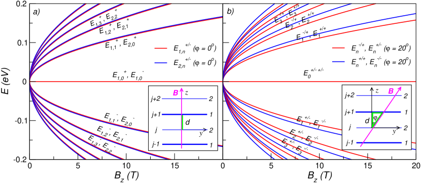
Figure 1: LLs of graphite at the H point as a function of the perpendicular component of the magnetic field, $B_{z}$. a) LLs, $E_{1,n}^{\pm}$ and $E_{2,n}^{\pm}$, in the perpendicular magnetic field ($\varphi=0^{o}$). b) LLs, $E_{n}^{\pm,\pm}$, splitted by tilting the magnetic field ($\varphi=20^{o}$).

Lifting of LL degeneracy by the tilted magnetic field is shown in Fig. 1. The LL splitting is of the order of several meV, and it grows with the tilt angle, i.e., with $B_{y}$.

To conclude, we have obtained the LL structure of graphite at the H point of the Brillouine zone in the tilted magnetic field configuration. This effect is experimentally observable.

References

• (1) S. S. Pershoguba and V. M. Yakovenko, Phys. Rev. B 82, 205408 (2010).
• (2) Y.-H. Hyun, Y. Kim, C. Sochichiu, M.-Y. Choi, arXiv:1008.0488v1 (2010).
• (3) M. Koshino and T. Ando, Phys. Rev. B 77, 115313 (2008).
• (4) M. Orlita, C. Faugeras, J. M. Schneider, G. Martinez, D. K. Maude, M. Potemski,
Phys. Rev. Lett. 102, 166401 (2009).
• (5) N. A. Goncharuk, L. Smrčka, J. Kučera, K. Výborný, Phys. Rev. B 71, 195318 (2005).