Scattering amplitudes: the most perfect microscopic structures in the universe

Abstract

This article gives an overview of many of the recent developments in understanding the structure of relativistic scattering amplitudes in gauge theories ranging from QCD to ${{\cal N}=4}$ super-Yang-Mills theory, as well as (super)gravity. I also provide a pedagogical introduction to some of the basic tools used to organize and illuminate the color and kinematic structure of amplitudes. This article is an invited review introducing a special issue of Journal of Physics A devoted to “Scattering Amplitudes in Gauge Theories”.

1 Overview

The astrophysicist Subrahmanyan Chandrasekhar once referred to black holes as “the most perfect macroscopic objects there are in the universe: the only elements in their construction are our concepts of space and time.” [1] This special issue of Journal of Physics A is devoted to a completely different topic, the quantum-mechanical amplitudes for the scattering of relativistic particles, in which a revolution in our understanding has been taking place recently. However, scattering amplitudes represent a kind of short-distance complement to the perfection Chandrasekhar saw in black holes. We might consider them to be the most perfect microscopic structures in the universe.

Black holes are gigantic and (almost) eternal. Scattering amplitudes, in contrast, portray events that wink in and out of existence much faster than the blink of an eye. They describe processes at the shortest distance scales that can be probed in the laboratory. When gravitons scatter, interacting via Einstein’s field equations, again in some sense the only elements in the construction are our concepts of space and time — although the boundary conditions at infinity can be more detailed than for black holes, involving multiple plane-wave ripples (the gravitons) propagating in various directions through Minkowski space-time. When other relativistic particles scatter, as in non-abelian gauge theory, more information has to be provided, such as the gauge group, the coupling constant, the matter content of the theory, the particle masses, and the precise set of particle types and spins being scattered. However, in the ultra-relativistic limit, if there are only gauge interactions, much of the group-theoretical information can be stripped from the amplitudes, and certain color-ordered “primitive” amplitudes can be defined which are quite universal. These amplitudes have intricate analytic properties, which have been teased out over the decades, but especially in the past few years. A variety of new, efficient techniques have been found to construct amplitudes, and hidden symmetries have been identified which illustrate the amplitudes’ “perfection.”

In the real universe, black holes are not found in an absolute vacuum. Typically they are surrounded by accretion disks of gas and dust, which muddy their perfection somewhat, but also enrich the range of phenomena involving them, and make them much easier to observe, albeit indirectly. Similarly, scattering amplitudes for quantum chromodynamics, or QCD, the most relativistic non-abelian gauge theory we can study in the laboratory, are shrouded from direct view by confinement. The quarks and gluons that theorists scatter mentally are never seen experimentally. In the initial state of a hadronic collision they are bound into a proton or other hadron. In the final state they emerge as collimated jets of particles. Despite this fact, quantities that are sensitive only to very short distances, so-called infrared-safe observables such as jet production cross sections, can be computed reliably in terms of quarks and gluons, in a systematic expansion in the strong coupling $\alpha_{s}$.

If we could go to asymptotically high energies, so that $\alpha_{s}$ were infinitesimal, it would be enough to consider just the leading order in this expansion, which is generated by the Born approximation, or tree-level amplitudes. The tree-level amplitudes of QCD have even more “perfection” than the generic, loop-level amplitudes, because they coincide with the tree amplitudes of a much more symmetric theory, ${{\cal N}=4}$ supersymmetric Yang-Mills theory (${{\cal N}=4}$ sYM). This theory, which is the subject of many of the articles in this special issue, has the maximum amount of supersymmetry possible in a gauge theory. Its four supercharges can be used to transform the helicity $+1$ gluon state, by $\frac{1}{2}$ unit of helicity at a time, all the way to the helicity $-1$ CPT conjugate gluon state. All states in the theory belong to a single supermultiplet, transforming in the adjoint representation of the gauge group. Therefore all interactions are related by supersymmetry to the triple-gluon vertex, and the theory has a single dimensionless coupling $g$. The $\beta$ function for ${{\cal N}=4}$ sYM vanishes exactly for any gauge group, $\beta(g)=0$, so that the theory is exactly conformally invariant at the quantum level, as well as classically. (The classical conformal invariance of QCD with massless quarks is of course spoiled by its nonvanishing one-loop $\beta$ function, which leads to asymptotic freedom.)

In investigations of scattering amplitudes in ${{\cal N}=4}$ sYM, the gauge group under consideration is usually SU$(N_{c})$. Quite often, the limit $N_{c}\to\infty$ is also taken, at a fixed value of the ’t Hooft coupling, $\lambda=g^{2}N_{c}$. For $\lambda\ll 1$, perturbation theory can be applied, and for large $N_{c}$ only planar Feynman diagrams contribute. For $\lambda\gg 1$, perturbation theory breaks down, but the AdS/CFT correspondence [2] can be used. In the large-$N_{c}$ or planar limit of ${{\cal N}=4}$ sYM, even more remarkable symmetries and relations emerge for scattering amplitudes. As we will discuss further below, these properties include dual conformal (super)symmetry, which is part of a larger Yangian invariance; a description of amplitudes in terms of spaces of complex planes (Grassmannians); and in terms of various types of twistors; and a relation between scattering amplitudes and the expectation values of Wilson loops for closed polygons bounded by light-like edges. Many of these properties are intimately connected with a strong-coupling picture of gluon scattering in terms of strings moving in anti-de-Sitter space [3].

The exceptional simplicity and numerous hidden symmetries of ${{\cal N}=4}$ sYM have made it a playground for theorists interested in scattering amplitudes for a couple of decades. This interest has accelerated rapidly in the past few years. Because the tree-level amplitudes of QCD and ${{\cal N}=4}$ sYM coincide, the early discoveries about QCD helicity amplitudes, motivated by the physics of jet production, were also discoveries about ${{\cal N}=4}$ sYM. For example, the Parke-Taylor formula [4] for the maximal-helicity-violating (MHV) sequence of $n$-gluon amplitudes, which is just a single-term expression, even for an arbitrarily large value of $n$, is also consistent with all the symmetries of ${{\cal N}=4}$ sYM [5], including some that were only unveiled decades later.

Many general properties of tree amplitudes were understood early on, such as their factorization properties [6] and the (${{\cal N}=1}$ or ${{\cal N}=2}$) supersymmetry Ward identities that they obey [7, 8]. However, a fuller understanding and exploitation of these properties have come only in recent years. For instance, the complete solutions of the long-known ${{\cal N}=4}$ supersymmetry Ward identities, and the corresponding ${{\cal N}=8}$ identities in supergravity, have been worked out recently by Elvang, Freedman and Kiermaier [9], and are reviewed here [10].

Several years ago, Witten [11] discovered that the twistor space developed decades earlier by Penrose [12] gave a natural description of tree-level amplitudes in massless gauge theory. As discussed in section 3, such amplitudes have a natural description in terms of two-component Weyl spinors, a left-handed and a right-handed spinor for each external state. To go to twistor space, one performs a Fourier transform on half the variables, namely the left-handed spinors, leaving the right-handed ones alone. Witten found that gauge theory could be reformulated in terms of a topological string moving in twistor space. Gauge amplitudes turn out to be localized on particular curves in twistor space. In one approach, the curves are intersecting lines: a single line for the simplest MHV amplitudes, a pair of lines for the next-to-maximally-helicity-violating (NMHV) amplitudes, and so on. This version gave rise to the CSW or MHV rules for gauge theory [13], whose MHV vertices are a particular off-shell continuation of the Parke-Taylor formulae. These developments are reviewed here by Brandhuber, Spence and Travaglini [14], and by Adamo, Bullimore, Mason and Skinner [15]. The latter reference also discusses another class of twistors, namely momentum twistors, which also provides a natural set of kinematic variables for amplitudes, in that they automatically satisfy the kinematic constraints of momentum conservation and the mass-shell conditions. Finally, the correspondence between Wilson loops and scattering amplitudes is described in this article [15] from the perspective of twistor space.

Britto, Cachazo, Feng and Witten (BCFW) [16] recognized that factorization properties are powerful enough to allow the derivation of recursion relations [17] for tree amplitudes, in terms of on-shell lower-point amplitudes, which are evaluated at particular complex momenta. This observation, reviewed here by Brandhuber, Spence and Travaglini [14], makes essential use of the analyticity, or plasticity, of amplitudes; that is, how they vary under smooth deformations of the kinematics. BCFW embedded an amplitude $A=A(0)$ into a one-complex-parameter family of on-shell amplitudes $A(z)$ with shifted complex momenta, and associated the poles of $A(z)$ in the $z$ plane with factorization of the amplitude onto simpler lower-point amplitudes. One can also construct a supersymmetrized version of the BCFW recursion relation, in which Grassmann variables $\eta^{A}$ associated with ${{\cal N}=4}$ supersymmetry are shifted along with the momenta [18, 19, 14]. This recursion relation can be solved explicitly to yield all tree amplitudes in ${{\cal N}=4}$ sYM [20]; the solution and its many symmetries are reviewed here by Drummond [21].

Scattering amplitudes in massless gauge theories all have quite similar structure at tree level, once the color factors have been stripped off, as discussed in section 2. On the other hand, the structure of loop amplitudes depends critically on the theory. The simplicity of one-loop multi-gluon amplitudes in ${{\cal N}=4}$ sYM played a key role in the development of the unitarity method [22, 23]. This method reconstructs loop amplitudes from their unitarity cuts, again exploiting analyticity. In general at one loop, as explained in this issue by Britto [24] and Ita [25], unitarity cuts are matched against a decomposition of the amplitude in terms of a set of scalar integrals — boxes, triangles, bubbles and (sometimes) tadpoles — in order to determine the coefficients of the integrals. In ${{\cal N}=4}$ sYM, the high degree of supersymmetry implies that only boxes have non-vanishing coefficients. Using unitarity, an infinite sequence of one-loop amplitudes (the MHV amplitudes) could be determined in ${{\cal N}=4}$ sYM from just the product of two tree-level MHV (Parke-Taylor) amplitudes [22].

Later, generalized unitarity was applied to the problem of computing one-loop amplitudes, by extracting additional information from products of three and four tree amplitudes, the so-called triple [26] and quadruple [27] cuts. Quadruple cuts have four on-shell conditions. These four equations determine the four components of the (four-dimensional) loop momenta completely, up to a (possible) two-fold degeneracy. This realization allows the box coefficients to be computed very simply in terms of the product of four tree amplitudes, glued together as the four corners of a box, and evaluated at each of the two solutions for the loop momenta [27]. For ${{\cal N}=4}$ sYM, there are no other coefficients to determine, so the one-loop problem has been “reduced to quadrature.” (It turns out that maximal ${{\cal N}=8}$ supergravity can be proven to have the same “no-triangle” property [28, 18], so it too is solved at one loop by the quadruple cuts.)

Generalized unitarity can also be applied very effectively at the multi-loop level. In principle it can be used for any gauge (or gravitational) theory. As an example, the two-loop four-gluon scattering amplitudes in QCD have been computed in this way [29]. In practice the method has been pushed the furthest in ${{\cal N}=4}$ sYM. The basic techniques of multi-loop generalized unitarity are reviewed here by Bern and Huang [30], and by Carrasco and Johansson [31].

Returning now to one-loop amplitudes for generic gauge theories, including QCD, the triangle and bubble coefficients have to be determined, as well as certain rational parts, which have no unitarity cuts in four dimensions. The triple cuts contain information about the triangle coefficients, but they also receive contributions from boxes. Similarly, the ordinary double cuts determine the bubble coefficients, once the contributions of triangles and boxes are removed. This separation can be done analytically, by making use of the different analytic behavior of the different types of cut integrals, as reviewed by Britto [24]. It can also be done numerically, by a suitable sampling of the continuum of loop momenta solving the triple or double cut on-shell conditions [32, 33, 34], as described by Ita [25]. These two articles also review methods for computing the rational parts of one-loop amplitudes. Although the rational parts have no unitarity cuts in four dimensions (by definition), they can be constructed via their cuts in dimensional regularization in $D=4-2\epsilon$ dimensions. Alternatively, it is possible to construct them recursively in the number of legs [34].

On-shell loop amplitudes in massless non-abelian gauge theories always contain infrared divergences, due to the exchange of soft gluons or virtual collinear splittings. In QCD it is conventional to regulate these divergences, as well as the ultraviolet ones, using dimensional regularization. In supersymmetric theories, dimensional reduction [35], or the related four-dimensional helicity scheme [36], can be used to keep the number of bosonic and fermionic states the same, and preserve Ward identities for ordinary supersymmetry.

The general structure of the infrared divergences is well understood from decades of work in QED as well as QCD [37]. It has been worked out in the most detail in the context of dimensional regularization [38, 39, 40]. The basic picture is shown in fig. 1. Soft divergences and collinear divergences associated with the amplitude $M$ each have a universal form. They can be factorized from each other and from a hard, short-distance part of the amplitude. Soft divergences, denoted by the blob marked $S$, come from exchange of long-wavelength gluons. These gluons do not have the resolving power to probe the internal structure of the “jets” $J$ of virtual collinear particles which capture the collinear divergences. Soft gluons can only see the overall color charges of the jets. An individual jet function $J_{i}$ depends on the type of particle $i$, but not on the full amplitude kinematics. The soft function $S$ does not depend on the particle types, but only on their momenta and color quantum numbers. In general these quantum numbers can be mixed by gluon exchange, so $S$ is a matrix in color space. The hard function $h$ has no infrared singularities, but generically depends on the particle types, colors and kinematics.

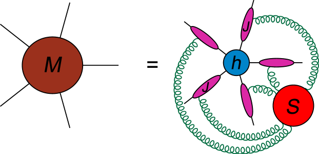
Figure 1: Factorization of soft and collinear singularities.

In the planar or large-$N_{c}$ limit, the picture simplifies considerably, to that shown in fig. 2. Now $M$ represents the coefficient of a particular color structure, such as $\,{\rm Tr}(T^{a_{1}}T^{a_{2}}\cdots T^{a_{n}})$ (assuming that all external states are in the adjoint representation; see section 2). In the planar limit, individual soft gluons can only connect color-adjacent external partons. There is no mixing of different color structures at large $N_{c}$. One can absorb the entire soft function $S$ into jet functions, which corresponds to breaking up the right-hand side of fig. 2 into $n$ wedges. Each wedge is bounded by two hard lines, and is composed of “half” of each of the two jet functions, as well as the soft gluons exchanged between them. Up to nonsingular terms, the wedge controlling the infrared divergences represents the square root of the Sudakov form factor, which is defined as the amplitude for a color-singlet state to decay into a pair of (adjoint) gluons.

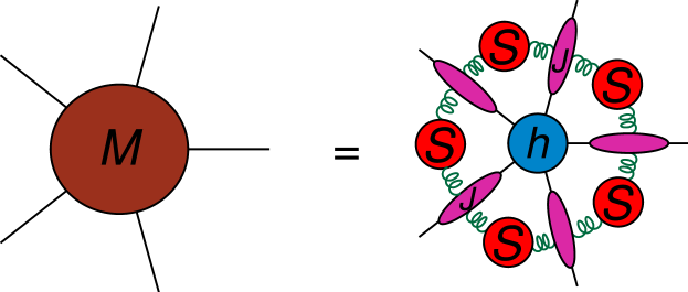
Figure 2: Soft-collinear factorization in the planar limit.

In dimensional regularization, the Sudakov form factor obeys a particular differential equation [38], whose source term is called the cusp anomalous dimension $\gamma_{K}$ [41]. There is an additional constant of integration, called ${\cal G}_{0}$. These two functions (along with the $\beta$ function in a non-conformal theory) control the infrared divergences to all orders for any amplitude in a planar massless gauge theory. In planar ${{\cal N}=4}$ sYM, the cusp anomalous dimension has been determined to all orders in the coupling using integrability [42]. The BDS ansatz [43] was built up from this description of the infrared singularities of planar amplitudes, plus the observation for the two- and three-loop four-point amplitudes that the hard function $h$ essentially reduces to a constant, independent of the kinematics.

Besides the cusp anomalous dimension, another place that integrability certainly enters multi-loop scattering amplitudes is in multi-Regge-kinematics, a particular class of high-energy or small-angle limits of $2\to(n-2)$ particle scatterings. These kinematics gave the first indication that the BDS ansatz for MHV amplitudes has to be corrected beginning at the six-point level [44]. (It was previously argued [45] using the properties of Wilson loops, that the ansatz should be corrected at two loops for a large value of $n$, unless the correspondence between MHV amplitudes and Wilson loops were to break down. The hexagon Wilson loop was then computed and found to differ from the ansatz prediction [46].) The dynamics of gluons in the transverse plane is given, in the leading-logarithmic approximation, by the Hamiltonian for a integrable open spin chain, as reviewed here by Bartels, Lipatov and Prygarin [47].

In planar ${{\cal N}=4}$ sYM, another infrared regulator is more convenient for many purposes, in particular for exploring the loop-level consequences of dual conformal symmetry, which is not preserved by dimensional regularization. The features of a recently-developed “Higgs regulator” [48] are reviewed in this issue by Henn [49]. For this regulator, vacuum expectation values are given to some of the adjoint scalar fields in the theory, breaking the gauge symmetry in such a way that (in the planar limit) the amplitudes are regulated by massive particles circulating around the outside of the loop diagrams. Dual conformal symmetry remains exact in a certain sense. When the particle masses $m_{i}$ are taken to be much less than the momentum-invariants for the scattering process, logarithmic divergences develop, the analogs of the $1/\epsilon$ infrared poles in dimensional regularization.

There is a hierarchy of simplicity in the scattering amplitudes for various types of gauge theory, as sketched in fig. 3. This hierarchy begins to be revealed at one loop. The outer region of the diagram stands for a generic gauge theory with massive matter fields, and perhaps massive gauge bosons, if the gauge symmetry is spontaneously broken, as in electroweak theory. One-loop amplitudes in such a theory generically contain tadpole integrals. One-particle cuts are nontrivial, and are particularly delicate because of external-leg contributions [50, 24]. The cut structure of loop integrals containing massive propagators in the loop is generically somewhat more complicated than the purely massless case. Massive particles in the loop can be unstable, which usually necessitates complex masses. When one enters the “massless” ring in fig. 3, corresponding to massless gauge bosons and matter fields, most of these complications vanish, although there are still generically rational parts to compute. The ring “sYM” stands for supersymmetric gauge theories. Their one-loop amplitudes can be constructed from four-dimensional unitarity cuts alone, i.e. there are no non-trivial rational parts [23].

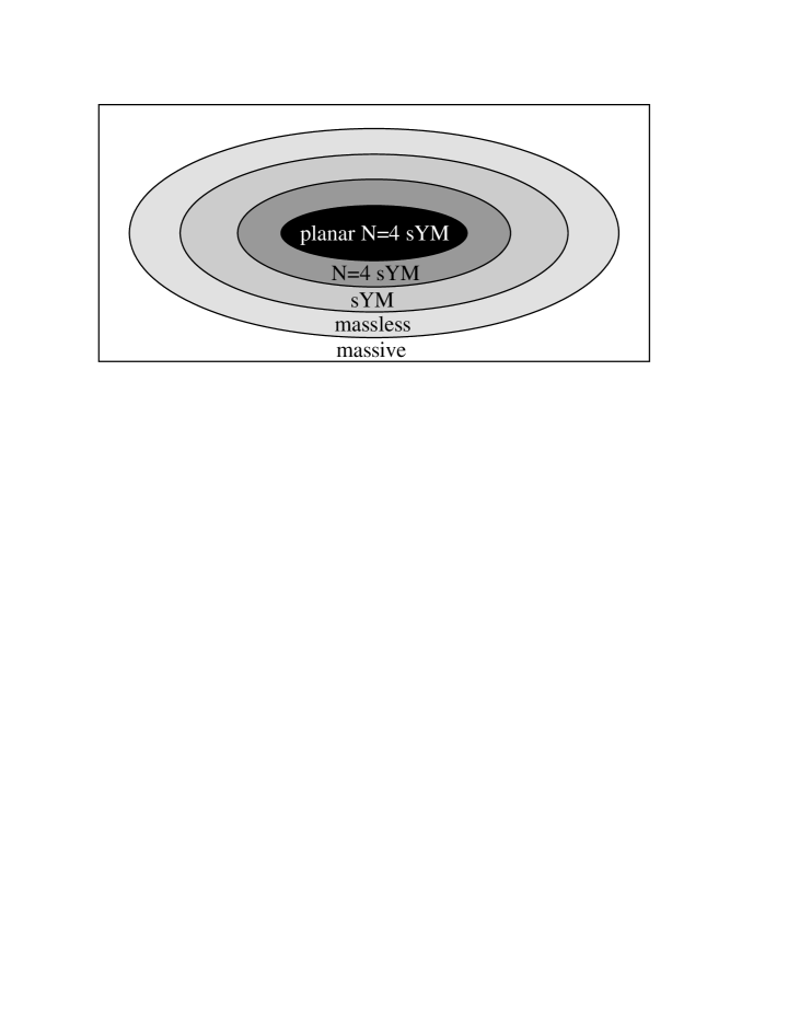
Figure 3: Hierarchy of simplicity in scattering amplitudes for various types of gauge theory.

Moving further inward in fig. 3, we arrive at ${{\cal N}=4}$ sYM. As mentioned earlier, at one loop the coefficients of bubble and triangle integrals now vanish, as well as the independent rational parts. (There are other gauge theories with vanishing bubble and triangle coefficients, at least for their $n$-gluon amplitudes [51, 24].) The theory becomes conformally invariant. It has been conjectured that the leading singularities — the multi-loop analogs of the quadruple cuts — are sufficient to determine the amplitudes at any loop order [18]. In addition, scattering amplitudes have empirically a predictable, uniform transcendental weight [52, 53]. This weight refers to their construction out of polylogarithms, logarithms, and Riemann $\zeta(n)$ values. For example, the finite (${\cal O}(\epsilon^{0})$) terms in one-loop ${{\cal N}=4}$ sYM amplitudes are of weight two: They contain some terms proportional to the polylogarithm ${\rm Li}_{2}$, and others which are products of two logarithms, or proportional to $\zeta(2)$, but they do not contain any terms of lower transcendentality. (At one loop this result just follows from the absence of bubble and tadpole integrals.) Wherever analytic results are available, this uniform transcendentality property holds. For example, at two loops (weight four for the finite terms) it holds for the non-planar, subleading-color terms as well as the planar ones [54].

Finally, for planar ${{\cal N}=4}$ sYM, as mentioned earlier, additional symmetries appear, dual superconformal invariance and an associated Yangian symmetry. The extra symmetries are related to integrability. They give rise to the prospect of adapting methods developed for other integrable systems to determine the $S$-matrix exactly, at least in the large $N_{c}$ limit. Indeed, as reviewed by Drummond [21], an integrand exhibiting manifest Yangian invariance has been proposed recently [55] for the general $L$-loop $n$-point amplitude, based on the BCFW recursion relations; see also ref. [56].

At the level of integrated amplitudes, dual conformal invariance has an anomaly due to the need for an infrared regulator. The anomaly was first understood in terms of Wilson loops rather than amplitudes [57] (for which divergences are ultraviolet in nature, rather than infrared). Nevertheless, dual conformal symmetry completely fixes the form of the four- and five-point amplitudes. The form to which they are fixed turns out to be precisely the ABDK/BDS ansatz [58, 43], which was developed earlier based on the structure of infrared divergences of amplitudes, plus patterns observed at two and three loops. As discussed in section 3.3, for six external legs one can build three different combinations of kinematic variables that are invariant under all dual conformal transformations, the cross-ratios $u_{1}$, $u_{2}$ and $u_{3}$. At the six-point level, the ABDK/BDS ansatz fails at the first nontrivial order, two loops [59], and dual conformal symmetry allows for an additional “remainder function”, $R_{6}^{(2)}(u_{1},u_{2},u_{3})$, which depends on the three cross-ratios.

At strong coupling, large $\lambda$ and large-$N_{c}$, Alday and Maldacena used the AdS/CFT correspondence to map the problem of gluon scattering to that of strings moving in anti-de-Sitter space [3]. The AdS background is weakly curved in this limit, relative to the string scale. Another way of saying this is that the two-dimensional string world-sheet stretches over a large area, relative to the scale on which strings fluctuate, allowing a semi-classical expansion to be used at large $\lambda$. In the leading term in the expansion, different helicity configurations are not distinguished. The amplitude is given simply by $\exp(-S_{\rm cl})$, where $S_{\rm cl}$ is the classical action that minimizes the area (at least for scattering configurations with a Euclidean interpretation). Using a $T$-duality transformation in string theory, Alday and Maldacena showed that the boundary conditions for the world-sheet are closed polygons, where each edge is a light-like segment given by the momentum $k_{i}$ of the $i^{\rm th}$ gluon. The solution to the minimal area problem was found explicitly for four-gluon scattering. More recently, in order to handle more complicated kinematical configurations than the four-point case, the integrability of the string sigma-model action [60] has been exploited. The minimal area problem has been solved by mapping it to a system of equations identical to those of the Thermodynamical Bethe Ansatz [61].

The first computation at strong coupling was for the four-gluon amplitude, and matched precisely the prediction of the ABDK/BDS ansatz [3]. But it also suggested a weak-coupling correspondence between scattering amplitudes and Wilson loops for closed light-like polygons, which was rapidly established for a variety of cases, initially for the simplest case of MHV scattering amplitudes [62, 57, 59]. The Wilson-loop correspondence has been very important both conceptually and technically. Conceptually, it is still not entirely clear why it happens at all at weak coupling. Technically, given its existence, it allows amplitudes to be computed in terms of Wilson line integrals, which are generally somewhat more tractable than Feynman loop integrals. Some recent conceptual advances have come from considering certain correlation functions with close-to-light-like separations [63, 15].

The relative simplicity of the Wilson line integrals for the six-point (hexagon) case allowed the remainder function $R_{6}^{(2)}(u_{1},u_{2},u_{3})$ to be evaluated analytically in terms of Goncharov polylogarithms [64]. The expression in ref. [64] was then simplified considerably, to a few lines involving classical polylogarithms ${\rm Li}_{m}$, using properties of the symbol operation which captures all of the essential analytic behavior of a multi-variable function [65]. These results open the door to the possibility of finding simple analytic results for more general kinematic configurations. For some configurations in which the external momenta are restricted to two space-time dimensions, two-loop analytic results are already available beyond six external legs [66]. There is certainly the prospect of more multi-loop analytic results on the horizon, for both Wilson loops and scattering amplitudes in planar ${{\cal N}=4}$ super-Yang-Mills theory.

Gravity seems to be a completely separate force from gauge theory. It has a spin two force carrier instead of spin one, no color degrees of freedom, and a dimensionful coupling constant. Nevertheless, the two theories are intimately connected. The AdS/CFT correspondence [2] relates the two, holographically, as a weak-strong duality. As mentioned earlier, strong-coupling scattering of gluons has an alternate description in terms of strings moving in a weakly-curved five-dimensional gravitational background. On the other hand, there is also a weak-weak duality of some kind between gravity and gauge theory, directly in four dimensions: It is possible to write perturbative scattering amplitudes for gravitons in terms of “double copies” of gluon amplitudes.

The original examples of such relations are due to Kawai, Lewellen and Tye (KLT) [67], who found them by first deriving relations between closed and open string theory tree amplitudes, whose low-energy limits give tree-level relations in field-theory. Graviton amplitudes are represented in terms of sums of products of pairs of gluon amplitudes with different color orderings. The KLT relations hold not only for pure-graviton scattering, in terms of pure-gauge theory, but also for ${{\cal N}=8}$ supergravity (or any subsector of it) in terms of amplitudes for ${{\cal N}=4}$ sYM. More recently it has been recognized that other double-copy formulas exist [68, 69]. The new formulas are simpler in some sense than the KLT relations; they involve the direct squares of gauge-theory components, whereas the KLT relations employ multiple permutations of full gauge-theory amplitudes. As reviewed in this issue by Carrasco and Johansson [31], these relations, combined with generalized unitarity, have important consequences for multi-loop amplitudes in ${{\cal N}=8}$ supergravity, because they map the problem to a much simpler one, the corresponding multi-loop amplitudes for (non-planar) ${{\cal N}=4}$ sYM.

In the next two sections we discuss a few of the basic tools used to organize and illuminate the color and kinematic structure of amplitudes, which underlay the discussions in many of the other articles in this special issue.

2 Color Preliminaries

In this section we describe some common conventions for organizing the color structure of SU$(N_{c})$ gauge theory amplitudes, which are used elsewhere in this special issue. Most of the articles implicitly discuss color-ordered partial amplitudes, which are particularly convenient in the large-$N_{c}$ limit in which planar diagrams dominate. Color-ordered amplitudes emerge from a “trace-based” color decomposition (as also reviewed in e.g. refs. [6, 70]). However, in some cases, in particular for describing subleading-color terms in amplitudes, and color-kinematic duality relations [31], decompositions based on the SU$(N_{c})$ structure constants are more useful.

In general, we consider two different SU$(N_{c})$ representations for the external states:

• The adjoint representation, for the gluon and any of its superpartners (i.e. for all states in ${{\cal N}=4}$ sYM). Adjoint color indices are denoted by $a,b,c,a_{i},\ldots\in\{1,2,\ldots,N_{c}^{2}-1\}$.

• The fundamental (defining) representation $N_{c}$, and its conjugate representation $\overline{N}_{c}$, for quarks and anti-quarks respectively. Fundamental color indices are denoted by $i_{1},i_{2},\ldots\in\{1,2,\ldots,N_{c}\}$, and anti-fundamental $\overline{N}_{c}$ indices by ${\bar{\jmath}}_{1},{\bar{\jmath}}_{2},\ldots\in\{1,2,\ldots,N_{c}\}$.

The generators of SU$(N_{c})$ in the fundamental representation are traceless hermitian $N_{c}\times N_{c}$ matrices, denoted by $(T^{a})_{i}^{{\bar{\jmath}}}$. It is conventional when discussing helicity amplitudes to normalize the generators by $\,{\rm Tr}(T^{a}T^{b})=\delta^{ab}$, in order to avoid a proliferation of $\sqrt{2}$’s.

In QCD, the group theory (color) factors in Feynman diagrams are of two types: $(T^{a})_{i}^{{\bar{\jmath}}}$ for the gluon-quark-antiquark vertex, and the SU$(N_{c})$ structure constants $f^{abc}$ (or products of $f^{abc}$’s) for all other vertices. (It is also convenient to normalize the structure constants differently, using $\tilde{f}^{abc}\equiv i\sqrt{2}f^{abc}$, where $f^{abc}$ is the standard, textbook normalization.) The color factors can be represented diagrammatically [71] using Feynman-diagram notation, as in fig. 4. Lines with arrows (quarks) carry fundamental representation indices; curly lines (gluons) carry adjoint indices. The adjoint representation is also a bi-fundamental ($N_{c}\times\overline{N}_{c}$) representation from which the singlet, or trace component, has been projected out, as in the second equation for $\delta^{ab}$ in the figure. This relation also gives rise to the SU$(N_{c})$ Fierz identity,

$$(T^{a})_{i_{1}}^{~{}{\bar{\jmath}}_{1}}\,(T^{a})_{i_{2}}^{~{}{\bar{\jmath}}_{2}}\ =\ \delta_{i_{1}}^{~{}{\bar{\jmath}}_{2}}\delta_{i_{2}}^{~{}{\bar{\jmath}}_{1}}-{1\over N_{c}}\,\delta_{i_{1}}^{~{}{\bar{\jmath}}_{1}}\delta_{i_{2}}^{~{}{\bar{\jmath}}_{2}}\,,$$ (1)

which allows one to simplify products of traces of $T^{a}$’s.

Figure 4: Graphical representation of building blocks for SU$(N_{c})$ color factors.

2.1 Trace-based color decompositions

Color-ordering [72] is related to the ’t Hooft double-line formalism [73]. We begin by rewriting the color factors entirely in terms of the $T^{a}$ generators, using the relation

$$\tilde{f}^{abc}\equiv i\sqrt{2}\,f^{abc}=\,{\rm Tr}([T^{a},T^{b}]T^{c})\,,$$ (2)

which follows from the definition of the structure constants, and is depicted graphically in fig. 4. After inserting eq. (2) repeatedly into the color factor for a typical Feynman diagram, one obtains a large number of traces of the generic form $\,{\rm Tr}\bigl{(}\ldots T^{a}\ldots\bigr{)}\,\,{\rm Tr}\bigl{(}\ldots T^{a}\ldots\bigr{)}\,\ldots\,\,{\rm Tr}\bigl{(}\ldots)$. If the amplitude has external quark legs, then there will also be strings of $T^{a}$’s terminated by fundamental indices, of the form $(T^{a_{1}}\ldots T^{a_{m}})_{i_{2}}^{~{}{\bar{\imath}}_{1}}$, one for each external quark-antiquark pair.

The number of traces can be reduced considerably by repeated use of the SU$(N_{c})$ Fierz identity (1). In the case of tree-level amplitudes with external states in the adjoint representation, such as $n$-gluon amplitudes, fig. 5 sketches how the color factors all may be reduced to a single trace, $\,{\rm Tr}\bigl{(}T^{a_{\sigma(1)}}T^{a_{\sigma(2)}}\cdots T^{a_{\sigma(n)}}\bigr{)}$, for some permutation $\sigma\in S_{n}$ of the $n$ gluons. This reduction leads to the trace-based color decomposition for $n$-gluon tree amplitudes,

$$\hskip-56.9055pt{\cal A}^{\rm tree}_{n}(\{k_{i},h_{i},a_{i}\})=g^{n-2}\hskip-3.69885pt\sum_{\sigma\in S_{n}/Z_{n}}\hskip-3.69885pt\,{\rm Tr}(T^{a_{\sigma(1)}}\cdots T^{a_{\sigma(n)}})\ A_{n}^{\rm tree}(\sigma(1^{h_{1}}),\ldots,\sigma(n^{h_{n}}))\,.$$ (3)

Here ${\cal A}^{\rm tree}_{n}$ is the full amplitude, with dependence on the external gluon momenta $k_{i}$, $i=1,2,\ldots,n$, helicities $h_{i}=\pm 1$, and adjoint indices $a_{i}$. In QCD, the gauge coupling $g$ is related to the strong coupling by $\alpha_{s}=g^{2}/(4\pi)$. The partial amplitudes (or primitive or color-stripped amplitudes) $A_{n}^{\rm tree}(1^{h_{1}},\ldots,n^{h_{n}})$ have had all the color factors removed, but contain all the kinematic information. Cyclic permutations of the arguments of a partial amplitude, denoted by $Z_{n}$, leave it invariant, because the associated trace is invariant under these operations. However, all $(n-1)!$ non-cyclic permutations, or orderings, of the partial amplitude appear in eq. (3). These permutations are denoted by $\sigma\in S_{n}/Z_{n}\equiv S_{n-1}$.

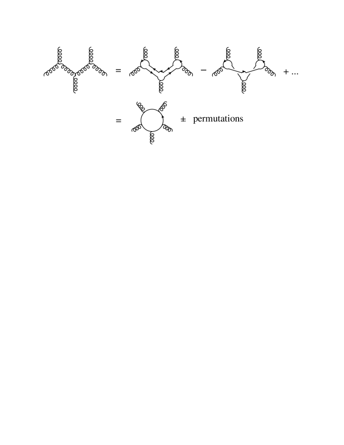
Figure 5: Reduction of color factors for $n$-gluon tree amplitudes to a single trace of $T^{a}$ generators.

Looking again at the way the different trace factors arise in fig. 5, one sees that the partial amplitude $A_{n}^{\rm tree}(1,2,\ldots,n)$ only receives contributions from tree-level Feynman diagrams that can be drawn on a plane, in which the cyclic ordering of the external legs, $1,2,\ldots,n$, matches the ordering of the arguments in $A_{n}^{\rm tree}$. Therefore each partial amplitude can only have singularities in momentum invariants formed by squaring color-adjacent sums of momenta, such as $s_{i,i+1}\equiv(k_{i}+k_{i+1})^{2}$, $s_{i,i+1,i+2}\equiv(k_{i}+k_{i+1}+k_{i+2})^{2}$, etc., where all indices are defined modulo $n$. In this way, the color decomposition (3) disentangles the kinematic complexity of the full amplitude ${\cal A}_{n}^{\rm tree}$.

Similarly, tree amplitudes with two external quarks and $(n-2)$ gluons can be reduced to single strings of $T^{a}$ matrices,

$${\cal A}^{\rm tree}_{n}(q_{1},g_{3},\ldots,g_{n-1},\bar{q}_{n}) = g^{n-2}\hskip-3.69885pt\sum_{\sigma\in S_{n-2}}\hskip-3.69885pt(T^{a_{\sigma(2)}}\cdots T^{a_{\sigma(n-1)}})_{i_{1}}^{~{}{\bar{\jmath}}_{n}}$$ (4)

$$\hskip 36.98866pt\hbox{}\times A_{n}^{\rm tree}(1_{q},\sigma(2),\ldots,\sigma(n-1),n_{\bar{q}}),$$

where we have omitted the helicity labels, and numbers without subscripts in the argument of $A_{n}^{\rm tree}$ refer to gluons. In this case there are $(n-2)!$ terms, corresponding to all possible gluon orderings between the quarks. Color decompositions for amplitudes containing additional external quark pairs have also been described [6].

We note that the partial amplitudes appearing in eq. (4) could also be used to describe the scattering of two fermions with different color quantum numbers, and $(n-2)$ gluons. For example, if the fermions are gluinos in the adjoint representation, then the color decomposition has the form of eq. (3), but the partial amplitudes, with two external fermions, are of the type given in eq. (4). This is easy to see if the two fermions are color-adjacent; essentially all one needs to do to go between the two cases is remove one color line running between the two gluinos. However, the other cyclic orderings can also be obtained from $A_{n}^{\rm tree}(1_{q},2,\ldots,n-1,n_{\bar{q}})$, using the Kleiss-Kuijf relations discussed in the next subsection. This property illustrates the universality of the color-ordered primitive amplitudes alluded to in the introduction.

Many articles in this issue consider loop-level amplitudes in which all of the external states are gluons in the adjoint representation. The general color decomposition here is similar to eq. (3), except that multiple color traces are now possible. Roughly speaking, a loop of gluons carries a fundamental and an anti-fundamental index around the loop with it, and an external gluon can attach to either index. The number of traces at $L$ loops is equal to $L+1$.

At one loop, the full color decomposition for $n$ gluons is [74]

$$\hskip-68.2866pt{\cal A}^{\rm 1\hbox{-}loop}_{n}(\{k_{i},h_{i},a_{i}\}) = g^{n}\Biggl{[}\sum_{\sigma\in S_{n}/Z_{n}}N_{c}\,\,{\rm Tr}(T^{a_{\sigma(1)}}\cdots T^{a_{\sigma(n)}})\ A_{n;1}(\sigma(1^{h_{1}}),\ldots,\sigma(n^{h_{n}}))$$ (5)

$$\hskip 14.22636pt+\ \sum_{c=2}^{\lfloor{n/2}\rfloor+1}\sum_{\sigma\in S_{n}/S_{n;c}}\,{\rm Tr}(T^{a_{\sigma(1)}}\cdots T^{a_{\sigma(c-1)}})\ \,{\rm Tr}(T^{a_{\sigma(c)}}\cdots T^{a_{\sigma(n)}})\$$

$$\hskip 122.34685pt\times\ A_{n;c}(\sigma(1^{h_{1}}),\ldots,\sigma(n^{h_{n}}))\Biggr{]}\,.$$

Here $A_{n;c}$ are the partial amplitudes, $Z_{n}$ and $S_{n;c}$ are the subsets of $S_{n}$ that leave the corresponding single and double trace structures invariant, and $\lfloor x\rfloor$ is the greatest integer less than or equal to $x$. The formula is more complicated than at tree level, but only by the need to keep track of more distinct trace structures and their various symmetries.

If there are $n_{f}$ flavors of quarks in the loop, it is easy to see that they only contribute to the single-trace coefficient $A_{n;1}$ in eq. (5), and with a weight $n_{f}/N_{c}$ relative to the adjoint gluons. (Similar color decompositions are available for one-loop amplitudes with an external quark pair [75].)

When one constructs the color-summed cross section, as is usually required for QCD applications, the contribution of the double-trace coefficients, $A_{n;c}$ for $c>1$, is suppressed by a power of $1/N_{c}^{2}$ with respect to that of $A_{n;1}$. (It also turns out that the $A_{n;c}$ are not really independent, but can be computed as a sum over permutations of the $A_{n;1}$ [22].) Thus eq. (5) simplifies a lot in the large-$N_{c}$ limit. The factor of $N_{c}=\,{\rm Tr}(1)$ simply comes from those terms in which all external gluons attach to the same fundamental index line, leaving the trace of the identity matrix for the untouched line.

Correspondingly, if we only want the leading terms in the large-$N_{c}$ limit at $L$ loops, we can write the compact color decomposition,

$$\hskip-42.67912pt{\cal A}^{L\rm\hbox{-}loop}_{n}(\{k_{i},h_{i},a_{i}\})|_{\rm leading\hbox{-}color}$$

$$\hskip-14.22636pt=g^{n-2}\,(g^{2}N_{c})^{L}\sum_{\sigma\in S_{n}/Z_{n}}\,{\rm Tr}(T^{a_{\sigma(1)}}\cdots T^{a_{\sigma(n)}})\ A_{n}^{(L)}(\sigma(1^{h_{1}}),\ldots,\sigma(n^{h_{n}}))\,,$$ (6)

where we have dropped the “;1” index on the leading-color partial amplitude. The ’t Hooft coupling $\lambda=g^{2}N_{c}$ emerges naturally in this limit. The articles in this issue about multi-loop amplitudes in planar ${{\cal N}=4}$ sYM are generally concerned with the $A_{n}^{(L)}$ in eq. (6). Because each loop integration typically brings a factor of $1/(4\pi)^{2}$ (or $1/(4\pi)^{2-\epsilon}$ when using dimensional regularization in $D=4-2\epsilon$), in some cases the precise normalizations of the $A_{n}^{(L)}$ will differ by this factor, as well as possibly other conventional factors.

2.2 $f$-based color decompositions

There is another type of color decomposition that is actually more useful than the above trace-based decomposition for addressing certain issues, and particularly for working beyond the large-$N_{c}$ approximation. We could call this approach the $f$-based decomposition, because it goes back to the original color factors built out of the structure constants $f^{abc}$. (Now we assume that all states are in the adjoint representation.) The diagrammatic representation of a general $f$-based color factor at tree level has the structure of a cubic tree graph, with vertices given by $\tilde{f}^{abc}$’s and propagators given by $\delta^{ab}$’s. However, these color factors are not all independent, due to the color Jacobi identity. This identity can be written in different ways. One way,

$$\tilde{f}^{dae}\tilde{f}^{bce}-\tilde{f}^{dbe}\tilde{f}^{ace}=\tilde{f}^{abe}\tilde{f}^{cde}\,,$$ (7)

which is also depicted in fig. 6, corresponds to the fact that the structure constants are also the SU$(N_{c})$ generators in the adjoint representation, $\tilde{f}^{abc}=(F^{b})_{ac}$, so that their commutator gives $\tilde{f}^{abe}$ contracted with $F^{e}$.

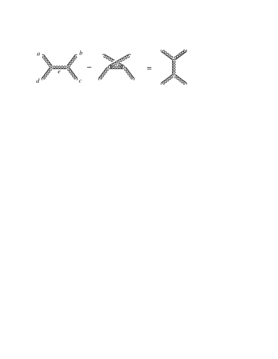
Figure 6: The Jacobi identity (7).

At tree level, one can use the identity (7) repeatedly to transform all $f$-based color factors into a “multi-peripheral” form in which two selected gluons, say 1 and $n$, are always at the end of a long chain of structure constants, and the other $(n-2)$ gluons are emitted from along the ladder [76, 77],

$$\hskip-56.9055pt{\cal A}_{n}^{\rm tree}(\{a_{i}\}) = g^{n-2}\sum_{\sigma\in S_{n-2}}\tilde{f}^{a_{1}a_{\sigma(2)}x_{1}}\tilde{f}^{x_{1}a_{\sigma(3)}x_{2}}\cdots\tilde{f}^{x_{n-3}a_{\sigma(n-1)}a_{n}}$$ (8)

$$\hbox{}\hskip 56.9055pt\times A_{n}^{\rm tree}(1,\sigma(2),\ldots,\sigma(n-1),n)\,$$

$$= g^{n-2}\sum_{\sigma\in S_{n-2}}(F^{a_{\sigma(2)}}\cdots F^{a_{\sigma(n-1)}})_{a_{1}a_{n}}A_{n}^{\rm tree}(1,\sigma(2),\ldots,\sigma(n-1),n)\,.$$

Notice that this representation is identical in form to the decomposition for two quarks and $(n-2)$ gluons in eq. (4), except for the representation used for the SU$(N_{c})$ generator matrices. Although eqs. (4) and (8) correspond to the cases of fundamental and adjoint representations, respectively, the same type of decomposition clearly holds for two external matter fields in an arbitrary SU$(N_{c})$ representation. The fact that the coefficients of the $f$-based decomposition (8) are identical to the color-ordered partial amplitudes $A_{n}^{\rm tree}$ appearing in the trace-based decomposition can be demonstrated by contracting both representations with $\,{\rm Tr}(T^{a_{1}}T^{a_{2}}\cdots T^{a_{n}})$ and keeping only the leading terms at large $N_{c}$ [77].

Note that there are only $(n-2)!$ terms in the $f$-based color decomposition, in contrast to the $(n-1)!$ terms in the trace-based decomposition (3). Therefore there are identities between the $A_{n}^{\rm tree}$, which are group-theoretical in nature — generalizations of certain $U(1)$ decoupling identities [6, 70]. These identities can be used to put any two legs next to each other, for example legs 1 and $n$:

$$A_{n}^{\rm tree}(1,\{\alpha\},n,\{\beta\})=(-1)^{n_{\beta}}\sum_{\sigma\in{\rm OP}\{\alpha\}\{\beta^{T}\}}A_{n}^{\rm tree}(1,\sigma(\{\alpha\}\{\beta^{T}\}),n)\,,$$ (9)

where $\{\alpha\}$ and $\{\beta\}$ are two sets of external gluons, whose union is $\{2,3,\ldots,n-1\}$. Also, $n_{\beta}$ is the number of elements in the set $\{\beta\}$, the set $\{\beta^{T}\}$ is $\{\beta\}$ with the ordering reversed, and ${\rm OP}\{\alpha\}\{\beta^{T}\}$ is the set of ordered permutations, or “mergings”, of the two sets $\{\alpha\}$ and $\{\beta^{T}\}$ that preserve the ordering of the $\alpha_{i}$ within $\{\alpha\}$ and of the $\beta_{i}$ within $\{\beta^{T}\}$, while allowing for all possible relative orderings of the $\alpha_{i}$ with respect to the $\beta_{i}$. These relations are known as the Kleiss-Kuijf relations [78]. They can be derived from eq. (8) by expanding out the $\tilde{f}^{abc}$ factors using eq. (2), identifying the coefficients of the trace structures, and comparing them with the original trace-based decomposition (3) [77].

In fact, it has been realized recently that there are not even $(n-2)!$ independent color-ordered amplitudes $A_{n}^{\rm tree}$, but only $(n-3)!$ [68], as reviewed in this issue by Carrasco and Johansson [31]. The additional linear relations between $A_{n}^{\rm tree}$’s are not purely group-theoretical in nature, but also involve kinematical factors. They allow one to put any three external gluon legs next to each other. For example, for legs 1, 2 and $n$, the identities take the form,

$$\hskip-28.45274ptA_{n}^{\rm tree}(\sigma(1),\sigma(2),\ldots,\sigma(n))=\sum_{\rho\in S_{n-3}}K^{(\sigma)}_{\rho}\,A_{n}^{\rm tree}(1,2,\rho(3),\ldots,\rho(n-1),n)\,,$$ (10)

where $\sigma$ and $\rho$ are permutations and $K^{(\sigma)}_{\rho}$ are kinematic-dependent (but not state-dependent) coefficients [68, 31]. These relations were first proved using open string theory [79], using a contour deformation argument [80] similar to that used in deriving the KLT relations [67] between gravity and gauge theory amplitudes. They have also been proven directly in field theory, using a recursive argument [81].

Although eq. (10) expresses the consequences of certain color-kinematic identities in the trace basis, the identities themselves are more naturally stated in an $f$-based approach. For this purpose it is useful to not transform the $f$-based color factors into multi-peripheral form, but leave the color decomposition free, in terms of the set of all cubic graphs $\Gamma_{3}$, writing

$${\cal A}_{n}^{\rm tree}=g^{n-2}\sum_{i\in\Gamma_{3}}\frac{N_{i}C_{i}}{(\prod_{j}p_{j}^{2})_{i}}\,.$$ (11)

The color factors $C_{i}$ are products of structure constants for each vertex $V_{i}$ of the $i^{\rm th}$ graph, contracted together along the propagators, $C_{i}=\prod_{j\in V_{i}}\tilde{f}^{a_{j_{1}}a_{j_{2}}a_{j_{3}}}$. The factors of $1/p_{j}^{2}$ are scalar propagators, one for each internal line in the graph, while the $N_{i}$ are kinematical numerator factors. Consider a triplet of graphs in $\Gamma_{3}$, which are identical except for a region from which four lines emanate. Within this region they differ according to the three ways of joining four legs with two cubic vertices, shown in fig. 6. Call the three graphs $s$, $t$ and $u$, and let the color factors $C_{s,t,u}$ be normalized (signed) so that they obey the Jacobi identity (7) as $C_{s}-C_{t}=C_{u}$. Then the statement of color-kinematic duality [68] is that the associated numerator factors should be related by $N_{s}-N_{t}=N_{u}$, for every such triplet of graphs. A simple and intuitive argument for these relations has been provided based on the heterotic string [82].

The existence of such a representation with local $N_{i}$ (i.e. polynomials in the momenta) has been checked in various examples, not only at tree level, but also through three loops for ${{\cal N}=4}$ sYM amplitudes [69]. As reviewed here by Carrasco and Johansson [31], the existence of a representation for gauge theory amplitudes satisfying $N_{s}-N_{t}=N_{u}$ for each triplet of Jacobi-related cubic graphs has important implications. Large classes of numerator factors are related to each other, and gravitational amplitudes are easily constructed from gauge theory ones.

3 Kinematic Preliminaries

Now that we have described two different ways to organize the color quantum numbers for scattering amplitudes, let us turn to kinematical issues, including convenient choices of external states and kinematical variables.

3.1 Spinor-helicity formalism

In QCD, the helicities of massless quarks are conserved by their chirality-preserving interactions with gluons. Hence it is natural to use a helicity basis for the quark amplitudes. In four-component notation, the spinors for the external states are taken to be $u_{\pm}(k)=\frac{1}{2}(1\pm\gamma_{5})u(k)$ for a quark with momentum $k$, and $v_{\mp}(k)=\frac{1}{2}(1\mp\gamma_{5})v(k)$ for an anti-quark. However, in the massless limit these spinors can be chosen to be equal to each other, $u_{\pm}(k)=v_{\mp}(k)$, and we can use two-component Weyl spinors as well. We will see that helicity amplitudes for external gluons can be built from the same objects.

We want to consider amplitudes with $n$ different momenta $k_{i}$, $i=1,2,\ldots,n$, and to do so in a way that respects crossing symmetry. Thus we take all the momenta to be outgoing, so that momentum conservation reads $\sum_{i}k_{i}^{\mu}=0$. In a realistic process with some incoming particles, the physical momentum for each of the incoming particles is simply the negative of the corresponding $k_{i}$. Also, the physical helicity $h_{i}$ is the negative of the one by which we label the amplitude. (The spin $S_{i}$ does not reverse under crossing, but $h_{i}=S_{i}\cdot k_{i}$ does.) The two-component spinor for the $i^{\rm th}$ state, if it is an outgoing fermion with helicity $\pm\frac{1}{2}$, has several notations [6, 70, 25]:

$$(\lambda_{i})_{\alpha}\ \equiv \ |i^{+}\rangle\ \equiv\ |k_{i}^{+}\rangle\ \equiv\ [u_{+}(k_{i})]_{\alpha}\ =\ [v_{-}(k_{i})]_{\alpha}\,,$$ (12)

$$(\tilde{\lambda}_{i})_{\dot{\alpha}}\ \equiv \ |i^{-}\rangle\ \equiv\ |k_{i}^{-}\rangle\equiv\ [u_{-}(k_{i})]_{\dot{\alpha}}\ =\ [v_{+}(k_{i})]_{\dot{\alpha}}\,.$$ (13)

Similarly, the conjugate spinors are

$$(\tilde{\lambda}_{i})^{\dot{\alpha}}\ \equiv \ \langle i^{+}|\ \equiv\ \langle k_{i}^{+}|\ \equiv\ [\overline{u_{+}(k_{i})}]^{\dot{\alpha}}\ =\ [\overline{v_{-}(k_{i})}]^{\dot{\alpha}}\,,$$ (14)

$$(\lambda_{i})^{\alpha}\ \equiv \ \langle i^{-}|\ \equiv\ \langle k_{i}^{-}|\ \equiv\ [\overline{u_{-}(k_{i})}]^{\alpha}\ =\ [\overline{v_{+}(k_{i})}]^{\alpha}\,.$$ (15)

Two-component indices are raised and lowered with the two-dimensional antisymmetric tensors $\epsilon^{\alpha\beta}$, $\epsilon^{\dot{\alpha}\dot{\beta}}$, etc. The spinor inner products come from contracting spinors for different momenta with these tensors,

$$\left\langle j\,l\right\rangle\ = \ \epsilon^{\alpha\beta}(\lambda_{j})_{\alpha}(\lambda_{l})_{\beta}\ =\ \langle j^{-}|l^{+}\rangle\ =\ \overline{u_{-}(k_{j})}u_{+}(k_{l})\,,$$ (16)

$$\left[j\,l\right]\ = \ \epsilon^{\dot{\alpha}\dot{\beta}}(\tilde{\lambda}_{j})_{\dot{\alpha}}(\tilde{\lambda}_{l})_{\dot{\beta}}\ =\ \langle j^{+}|l^{-}\rangle\ =\ \overline{u_{+}(k_{j})}u_{-}(k_{l})\,.$$ (17)

Spinor products are antisymmetric under exchange of labels, $\left\langle j\,l\right\rangle=-\left\langle l\,j\right\rangle$, $\left[j\,l\right]=-\left[l\,j\right]$, and $\left\langle j\,j\right\rangle=\left[j\,j\right]=0$. Lorentz vectors can be written as bi-spinors, or $2\times 2$ matrices, by contracting them with the Pauli matrices. A massless vector written in this way factorizes into the product of two massless spinors, as

$$({\raise 0.97221pt\hbox to5.52084pt{\hss/\hss}\hbox to0.0pt{\hss$k$}}_{i})_{\alpha\dot{\alpha}}\ \equiv\ k_{i}^{\mu}(\sigma_{\mu})_{\alpha\dot{\alpha}}\ =\ u_{+}(k_{i})\overline{u_{+}(k_{i})}\ =\ (\lambda_{i})_{\alpha}(\tilde{\lambda}_{i})_{\dot{\alpha}}\,.$$ (18)

This factorization plays a role in the BCFW complex-momentum shift, which is best described in terms of the $\lambda$ and $\tilde{\lambda}$ variables [16], as is done elsewhere in this issue [14, 25, 21].

Amplitudes with external gluons can also be described in terms of the $\lambda_{i}$ and $\tilde{\lambda}_{i}$ variables, thanks to the spinor-helicity formalism [83]. The polarization vector $\varepsilon^{\pm}(k)$ for an outgoing massless vector particle with momentum $k$ and helicity $h=\pm 1$, is required to be transverse to $k$, $\varepsilon^{\pm}\cdot k=0$. In the spinor-helicity formalism, $\varepsilon^{\pm}$ is also chosen to be transverse to another massless momentum $q$, called the reference momentum (which should not be parallel to $k$ but is otherwise arbitrary). Note that $k$ and $q$ span a two-dimensional subspace of four-dimensional space-time. Because ${\raise 0.97221pt\hbox to5.52084pt{\hss/\hss}\hbox to0.0pt{\hss$k$}}|k^{\pm}\rangle={\raise-1.31944pt\hbox to4.8229pt{\hss/\hss}\hbox to0.0pt{\hss$q$}}|q^{\pm}\rangle=0$, the two orthogonal directions to this subspace are spanned by $\langle q^{+}|\gamma^{\mu}|k^{+}\rangle$ and $\langle q^{-}|\gamma^{\mu}|k^{-}\rangle$. The spinor-helicity polarization vectors live in this subspace; indeed, they are proportional to these two vectors, and are normalized by the condition that $\varepsilon^{\pm}\cdot(\varepsilon^{\pm})^{*}=-1$:

$$\varepsilon_{\mu}^{\pm}(k,q)=\pm\frac{\langle q^{\mp}|\gamma_{\mu}|k^{\mp}\rangle}{\sqrt{2}\langle q^{\mp}|k^{\pm}\rangle}\,.$$ (19)

As a bi-spinor, $\varepsilon^{\pm}(k_{i},q_{i})$ is given by

$$\hskip-28.45274pt[\varepsilon^{+}(k_{i},q_{i})]_{\alpha\dot{\alpha}}=\sqrt{2}\frac{(\lambda_{q_{i}})_{\alpha}(\tilde{\lambda}_{i})_{\dot{\alpha}}}{\left\langle q_{i}\,i\right\rangle}\,,\qquad[\varepsilon^{-}(k_{i},q_{i})]_{\alpha\dot{\alpha}}=-\sqrt{2}\frac{(\lambda_{i})_{\alpha}(\tilde{\lambda}_{q_{i}})_{\dot{\alpha}}}{\left[q_{i}\,i\right]}\,.$$ (20)

If each $q_{i}$ is chosen to be another momentum in the process, say $k_{j}$, then it is clear from the general form of the Feynman rules (using also eq. (18)) that the full amplitude can be built entirely out of the spinor products $\left\langle j\,l\right\rangle$ and $\left[j\,l\right]$, for $1\leq j,l\leq n$.

What are the basic properties of the spinor products which make them so convenient variables for helicity amplitudes? First of all, for real momenta, the two types of spinor products are complex conjugates of each other, $\left\langle j\,l\right\rangle=\pm{\left[l\,j\right]}^{*}$. Also, for either real or complex momenta they “square” to give the ordinary dot products of momenta,

$$\left\langle l\,j\right\rangle\left[j\,l\right]\ =\ \,{\rm Tr}[\textstyle{\frac{1}{2}}(1-\gamma_{5}){\raise 0.97221pt\hbox to5.52084pt{\hss/\hss}\hbox to0.0pt{\hss$k$}}_{l}{\raise 0.97221pt\hbox to5.52084pt{\hss/\hss}\hbox to0.0pt{\hss$k$}}_{j}]\ =\ 2k_{j}\cdot k_{l}=s_{jl}\,.$$ (21)

(Equation (21) is written in the convention usually used in the QCD literature, but the reader should be aware that another convention exists, in which the sign of $\left[j\,l\right]$ is reversed so that $\left\langle l\,j\right\rangle\left[j\,l\right]=-s_{jl}$.)

For real momenta, the conjugation property and eq. (21) imply that

$$\left\langle j\,l\right\rangle\ =\ \sqrt{s_{jl}}\,e^{i\phi_{jl}}\,,\qquad\left[j\,l\right]\ =\ \sqrt{s_{jl}}\,e^{-i\phi_{jl}}\,,$$ (22)

where $\phi_{jl}$ is a phase. This phase shifts as $k_{j}$ and $k_{l}$ are rotated in azimuthal angle around the axis corresponding to their sum, $k_{P}=k_{j}+k_{l}$. One way of seeing the utility of the spinor products for helicity amplitudes is to examine the limits in which two particles become collinear, $k_{P}^{2}=s_{jl}\to 0$. Figure 7(a) shows that the typical behavior of amplitudes in a massless scalar field theory is $\sim 1/k_{P}^{2}=1/s_{jl}$, coming just from the scalar propagator. However, in massless gauge theory, there are numerator factors in the Feynman diagrams which lessen this divergence. More physically, the factorization in the collinear limit should be onto a physical gluon state with helicity $\pm 1$. However, the sum of the two external helicities must be $\pm 2$ or 0. Therefore there is at least a $\pm 1$ mismatch of the spin angular momentum along the $k_{P}$ axis, as illustrated in fig. 7(b). The spin angular-momentum mismatch requires some orbital angular momentum, which in turn causes a suppression of the magnitude of the amplitude, from $1/s_{jl}$ to $1/\sqrt{s_{jl}}$. It also dictates a phase shift under azimuthal rotation of $k_{j}$ and $k_{l}$ about the $k_{P}$ axis. Both of these properties are captured by the spinor products, making them ideal for describing helicity amplitudes.

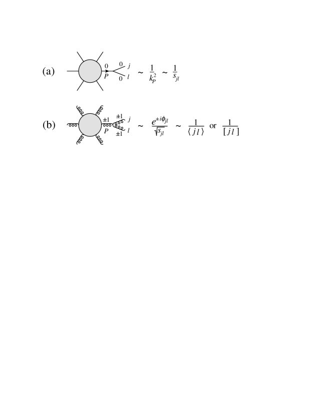
Figure 7: (a) A typical collinear limit in a theory with massless scalars. There is no suppression of the singularity from angular-momentum conservation. (b) A typical collinear limit in a massless gauge theory, for which there is always a mismatch of at least one unit of angular momentum, lessening the singularity.

The simplest nonvanishing tree-level gluon amplitudes are the Parke-Taylor or MHV amplitudes [4],

$$A_{n}^{\rm tree}(1^{+},\ldots,l^{-},\ldots,m^{-},\ldots,n^{+})=i\,{{\left\langle l\,m\right\rangle}^{4}\over\left\langle 1\,2\right\rangle\left\langle 2\,3\right\rangle\cdots\left\langle n\,1\right\rangle}\,.$$ (23)

Here exactly two gluons, $l$ and $m$, have negative helicity, and the remaining $(n-2)$ gluons have positive helicity. The amplitudes with zero or one negative gluon helicity vanish by supersymmetry Ward identities [7, 8]. The only denominator factors in these amplitudes are the spinor products for color-adjacent pairs of momenta, $\langle i,\,i+1\rangle$. They capture such universal collinear limits [6, 22] as,

$$\hskip-28.45274ptA_{n}^{\rm tree}(1^{+},\ldots,l^{-},\ldots,m^{-},\ldots,(n-1)^{+},n^{+})|_{n-1\parallel n}$$ (24)

$$\sim \frac{1}{\sqrt{z(1-z)}\langle n-1,\,n\rangle}\,A_{n-1}^{\rm tree}(1^{+},\ldots,l^{-},\ldots,m^{-},\ldots,P^{+})\,,$$ (25)

where legs $(n-1)$ and $n$ are becoming parallel, with $k_{P}=k_{n-1}+k_{n}$, $k_{n-1}\approx zk_{P}$ and $k_{n}\approx(1-z)k_{P}$.

3.2 Three-point amplitudes and complex kinematics

Another way to see why the spinor products are so useful is to consider the special case $n=3$ for the MHV amplitudes,

$$A_{3}^{\rm tree}(1^{-},2^{-},3^{+})=i\,{{\left\langle 1\,2\right\rangle}^{4}\over\left\langle 1\,2\right\rangle\left\langle 2\,3\right\rangle\left\langle 3\,1\right\rangle}\,.$$ (26)

One might think that the scattering of three massless particles is singular, because all of the $s_{jl}$ vanish since they are equal to the squared momentum of the remaining particle. Indeed, for real momenta, eq. (22) implies that all the spinor products vanish too, and there is no way to build a nonvanishing and nonsingular amplitude. However, for complex momenta, the complex-conjugation relation $\left\langle j\,l\right\rangle=\pm{\left[l\,j\right]}^{*}$ no longer holds, and it is possible for half the spinor products to be nonvanishing, while the other half vanish.

Specifically, we can choose the three negative-helicity two-component spinors to be proportional [11],

$$\tilde{\lambda}_{1}^{\dot{\alpha}}\ \propto\ \tilde{\lambda}_{2}^{\dot{\alpha}}\ \propto\ \tilde{\lambda}_{3}^{\dot{\alpha}}\,.$$ (27)

Then according to eq. (17) we have $\left[1\,2\right]=\left[2\,3\right]=\left[1\,3\right]=0$. However, the other three spinor products, $\left\langle 1\,2\right\rangle$, $\left\langle 2\,3\right\rangle$ and $\left\langle 1\,3\right\rangle$, are allowed to be nonzero. (This is consistent with the vanishing of eq. (21), which still holds for complex momenta.) For this choice of complex kinematics, the MHV three-point amplitude (26) is nonvanishing and nonsingular, while the conjugate “$\overline{{\rm MHV}}$” amplitude,

$$A_{3}^{\rm tree}(1^{+},2^{+},3^{-})=-i\,{{\left[1\,2\right]}^{4}\over\left[1\,2\right]\left[2\,3\right]\left[3\,1\right]}\,,$$ (28)

vanishes. In contrast, for the conjugate kinematics with

$$\lambda_{1}^{\alpha}\ \propto\ \lambda_{2}^{\alpha}\ \propto\ \lambda_{3}^{\alpha}\,,$$ (29)

eq. (26) vanishes while eq. (28) is nonvanishing and nonsingular.

The three-point amplitudes (26) and (28), as well as related amplitudes with two matter particles and one gluon, are very important in massless gauge theory. The BCFW relations build all tree-level scattering amplitudes recursively from them, using factorization onto multi-particle poles, as well as onto complex-momentum versions of the collinear poles shown in fig. 7. Of course Feynman diagrams can also be used to build amplitudes from three- and four-point vertices. However, Feynman vertices are typically evaluated with off-shell lines emanating from them, which makes them gauge-dependent. In contrast, eqs. (26) and (28) are on shell, albeit for complex momenta, and therefore they are fully gauge invariant. In the recursive construction of $n$-gluon amplitudes, the four-gluon vertex is never needed, essentially because it is related to the three-vertex by gauge transformations.

Another reason why the three-point amplitudes are important is for building up loop amplitudes through generalized unitarity, as reviewed in this issue by Ita [25] and Britto [24] at one loop, and by Bern and Huang [30] and Carrasco and Johansson [31] at the multi-loop level. Typically, generalized unitarity cuts place many propagators on shell, so they very often contain at least one three-point tree amplitude. Finally, the relations between gravity and gauge theory tree amplitudes are the simplest of all for the three-point case, where they can be written as an exact square,

$$M_{3}^{\rm tree}(1,2,3)=[A_{3}^{\rm tree}(1,2,3)]^{2}\,,$$ (30)

ignoring overall coupling-constant factors.

3.3 Kinematic variables for planar theories

For planar (large $N_{c}$) gauge theory amplitudes — which includes all tree-level amplitudes — new sets of kinematic variables have proved very useful for identifying new structures and symmetries.

Because the external legs have a definite cyclic order in the planar case, they carve the plane into sectors. To each such sector, one can assign a vertex $x_{i}^{\mu}$ for a dual graph, as shown in fig. 8(a). Lines connecting vertices of the dual graph cross lines of the original graph. The latter lines carry momenta. Differences between $x_{i}$’s are computed according to the net momentum flowing through the lines of the original graph. Thus in fig. 8(a), adjacent sectors are separated by $x_{j+1}-x_{j}=k_{j}$, or more generally,

$$x_{i,j}^{\mu}\equiv x_{i}^{\mu}-x_{j}^{\mu}=k_{j}^{\mu}+k_{j+1}^{\mu}+\cdots+k_{i-1}^{\mu}\,.$$ (31)

The $x_{i}$ are often called dual coordinates (or sometimes region or sector variables), but they are essentially momenta, not coordinates. In a planar loop graph we can assign additional $x_{i}$ variables to the faces inside each loop, corresponding to the independent loop momenta. Figure 8(b) shows a two-loop example. Here the thick lines of the dual graph that are shown each cross (and therefore correspond to) one propagator of the planar double box integral.

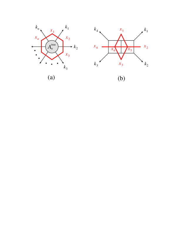
Figure 8: (a) Dual coordinates $x_{i}$ for a color-ordered tree amplitude with external momenta $k_{i}$. The dual variables live in the sectors, or regions, demarcated by the $k_{i}$. Thin (black) lines denote ordinary momenta, while thick (red) lines denote differences $x_{i,j}$ between dual coordinates. These differences also equal the momenta carried by the lines they cross. (b) Dual coordinates for a particular integral entering the planar two-loop four-gluon amplitude. Now additional dual coordinates, $x_{5}$ and $x_{6}$, live within the loops. In this case we only show the seven dual coordinate separations associated with the seven propagators for this integral ($x_{1,5}$, $x_{2,5}$, $x_{3,5}$, $x_{1,6}$, $x_{3,6}$, $x_{4,6}$ and $x_{5,6}$).

More precisely, differences of the $x_{i}$ are momenta. The $x_{i}$ themselves are not constrained by momentum conservation. They are constrained by on-shell conditions, $x_{j+1,j}^{2}=k_{j}^{2}=0$. However, unlike momenta, it is possible to invert the $x_{i}$’s, according to

$$x_{i}^{\mu}\to\frac{x_{i}^{\mu}}{x_{i}^{2}}\,,\qquad x_{i,j}^{2}\to\frac{x_{i,j}^{2}}{x_{i}^{2}x_{j}^{2}}\,.$$ (32)

Remarkably, this inversion is a symmetry of both integrands and amplitudes in planar ${{\cal N}=4}$ sYM. The integrands are functions of the combinations $x_{i,j}^{2}$, which are manifestly invariant under Lorentz transformations and translations of the $x_{i}$’s. (Translation invariance is guaranteed simply because the amplitude depends on momenta, which are differences of $x_{i}$’s.) Therefore the inversion (32) combines with Poincaré invariance to generate the conformal group SO(4,2). This group acts on the dual variables $x_{i}$, not on space-time coordinates; hence the symmetry is referred to as dual conformal invariance.

At the loop level, dual conformal invariance can be spoiled by the infrared regulator needed for on-shell amplitudes. A loop-integration measure in four dimensions, $d^{4}x_{i}$, transforms under an inversion (32) as, $d^{4}x_{i}\to d^{4}x_{i}/(x_{i}^{2})^{4}$. In $D=4$ this factor precisely cancels terms from inverting the associated propagators in graphs such as the one in fig. 8(b). However, in dimensional regularization, we have $D=4-2\epsilon$, and the invariance is lost due to extra factors in the transformation of the loop integration measure. As discussed in detail in this issue by Henn [49], for planar ${{\cal N}=4}$ sYM it is possible to retain dual conformal invariance at the loop level by using instead a Higgs regulator [48], which generates particle masses that can also be thought of as extra components of the $x_{i}^{\mu}$. Although amplitude computations with the Higgs regulator have not been pushed quite as far yet as in dimensional regularization, there are certain advantages to this approach. For example, in dimensional regularization, terms in lower-loop amplitudes that vanish as $\epsilon\to 0$ often have to be computed, because they can multiply pole terms, $\sim 1/\epsilon^{k}$, in other amplitudes (or in the squares of amplitudes needed to construct differential cross sections). The article by Schabinger in this issue discusses such ${\cal O}(\epsilon)$ contributions [84]. In contrast, with the Higgs regulator, the singularities have the form of powers of logarithms, $\sim\ln^{k}m^{2}$, and power-suppressed terms of the form $m^{2}/s_{i,i+1}$ can always be dropped, because they vanish faster than any power of a logarithm.

How constraining is dual conformal symmetry? In general it can only determine amplitudes up to arbitrary functions of the cross-ratios,

$$u_{ijkl}\ \equiv\ \frac{x_{ij}^{2}x_{kl}^{2}}{x_{ik}^{2}x_{jl}^{2}}\,,$$ (33)

because these variables are invariant under the inversion (32). However, the on-shell constraints $x_{i,i+1}^{2}=k_{i}^{2}=0$ imply that there are no non-trivial cross ratios for four- and five-particle scattering. At the six-point level there are three non-trivial cross ratios, utilizing the allowed $x_{i,i+2}^{2}$ and $x_{i,i+3}^{2}$ kinematic invariants:

$$\hskip-51.21504ptu_{1}=\frac{x_{13}^{2}x_{46}^{2}}{x_{14}^{2}x_{36}^{2}}=\frac{s_{12}s_{45}}{s_{123}s_{345}}\,,\quad u_{2}=\frac{x_{24}^{2}x_{51}^{2}}{x_{25}^{2}x_{41}^{2}}=\frac{s_{23}s_{56}}{s_{234}s_{123}}\,,\quad u_{3}=\frac{x_{35}^{2}x_{62}^{2}}{x_{36}^{2}x_{52}^{2}}=\frac{s_{34}s_{61}}{s_{345}s_{234}}\,.$$ (34)

As mentioned earlier, the remainder function $R_{6}^{(2)}$ characterizing the two-loop MHV six-point amplitude in planar ${{\cal N}=4}$ sYM is a function of these three variables, and this function is now known analytically in terms of polylogarithms [64, 65].

In planar ${{\cal N}=4}$ sYM, dual conformal invariance combines with dual ${{\cal N}=4}$ supersymmetry to generate dual superconformal symmetry [85, 86, 87]. It is natural to consider super-amplitudes, which package sets of amplitudes together by using an ${{\cal N}=4}$ on-shell superfield [5],

$$\hskip-65.44142pt\Phi(\eta)=g^{+}+\eta^{A}\,{\tilde{g}}_{A}+\frac{1}{2}\eta^{A}\eta^{B}\,\phi_{AB}+\frac{1}{3!}\eta^{A}\eta^{B}\eta^{C}\epsilon_{ABCD}\,{\bar{\tilde{g}}}^{D}+\frac{1}{4!}\eta^{A}\eta^{B}\eta^{C}\eta^{D}\epsilon_{ABCD}\,g^{-}.$$ (35)

Here $g^{\pm}$ are the $\pm 1$ helicity gluons, ${\tilde{g}}_{A}$ and $\bar{\tilde{g}}^{A}$ the four flavors of $\pm\frac{1}{2}$ helicity gluinos, and $\phi_{AB}$ the six real $0$ helicity scalar states. Integrations over the Grassmann variables $\eta^{A}$, $A=1,2,3,4$, can be used to pick off the desired component amplitudes from the super-amplitudes, defined by

$${\cal A}_{n}(\eta_{i})\ \equiv\ {\cal A}\Bigl{(}\Phi_{1}(\eta_{1}),\ldots,\Phi_{n}(\eta_{n})\Bigr{)}\,.$$ (36)

Just as the $x_{i}$ bosonic variables automatically satisfy momentum conservation, $k\equiv\sum_{i=1}^{n}k_{i}=0$, one can construct their superpartners $\theta_{i}^{A\alpha}$, whose differences satisfy

$$\theta_{i}^{A\alpha}-\theta_{i+1}^{A\alpha}\ =\ \lambda_{i}^{\alpha}\eta_{i}^{A}\,,$$ (37)

for $i=1,2,\ldots,n$. Super-momentum conservation constitutes eight constraints:

$$q^{A\alpha}\ \equiv\ \sum_{i=1}^{n}\lambda_{i}^{\alpha}\eta_{i}^{A}\ =\ 0.$$ (38)

Like ordinary momentum conservation, it is satisfied by virtue of the periodicity of the dual coordinates, $x_{i}\equiv x_{i+n}$, $\theta_{i}^{A\alpha}\equiv\theta_{i+n}^{A\alpha}$. The MHV super-amplitude generalizing eq. (23) is

$${\cal A}_{n}^{{\rm tree},{\rm MHV}}=i\frac{\delta^{4}(k)\,\delta^{8}(q)}{\left\langle 1\,2\right\rangle\left\langle 2\,3\right\rangle\cdots\left\langle n\,1\right\rangle}=i\frac{\delta^{4}(x_{1}-x_{n+1})\,\delta^{8}(\theta_{1}-\theta_{n+1})}{\left\langle 1\,2\right\rangle\left\langle 2\,3\right\rangle\cdots\left\langle n\,1\right\rangle}\,.$$ (39)

It transforms covariantly under dual superconformal transformations [85, 21] which extend SO(4,2) to the superalgebra PSU(2,2$|$4). Furthermore, the solutions to the BCFW super-recursion relation for amplitudes with more negative helicities (NMHV, NNMHV, etc.) are given by the product of this super-amplitude with collections of dual superconformal invariants, generically denoted by $R_{n}$ [85, 20, 21].

Superconformal and dual superconformal symmetry are separate symmetries, which partly overlap. They close into a very large symmetry group called the Yangian [88], as discussed in this issue by Bargheer, Beisert and Loebbert [89] and by Drummond [21]. The generic generator of the Yangian is not local in the sense of being a sum of single-particle terms (like $k$ and $q$); rather it is a sum of multi-particle operators. (For the dual superconformal generators, the nonlocality is mild; only the sum of two-particle operators appears.) There are certain “anomalies” in the action of the Yangian on amplitudes. At tree level, the anomalies only act at the boundary of the $n$-particle phase space, where two particles become collinear, as in fig. 7 [90]. At loop-level they act in the full phase-space, due to singularities in the loop integration [91]. However, it is possible to deform either the symmetry algebra or the representation in a suitable way so as to preserve the invariance [90, 91, 89]. It will be very interesting to see whether the constraints from the Yangian are sufficient to determine multi-loop amplitudes directly, without having to pass through the computation of loop integrals.

Another very recent development, in the same vein of using symmetries or dynamical principles to bypass standard loop (or Wilson line) integrals, concerns polygonal Wilson loops. One considers an operator-product-like expansion for the Wilson loop, associated with a limit in which multiple momenta become collinear [92]. This expansion can be carried out at both weak and strong coupling. At weak coupling it has been used to compute the discontinuity of the integrated two-loop amplitude, directly in terms of one-loop quantities [93].

4 Outlook

There has been a remarkable array of breakthroughs in our understanding of scattering amplitudes over the past few years, as described in the review articles in this special issue of Journal of Physics A. This article has represented an overview of many of these developments, as well as providing some basic material as an introduction to the remaining contributions. However, it certainly did not do justice to all of the directions being pursued currently.

One of the other remarkable features of this field has been the interplay and cross-fertilization between formal developments and phenomenology. The Parke-Taylor tree amplitudes were found in the course of trying to understand patterns arising in the structure of five- and six-gluon tree-level amplitudes. A similar analysis of the structure of the five-gluon amplitude at one loop in QCD led to the development of the unitarity method, which has been indispensable for computing high-loop-order amplitudes in maximally supersymmetric gauge theory and gravity, but which has also produced new NLO QCD results for colliders [25]. A “radiation zero” found over thirty years ago in the electroweak process $d\bar{u}\to W^{-}\gamma$ [94] was studied for a general gauge theory soon thereafter [95]; the relations found there were recognized much later as the four-point versions of a more general color-kinematics duality [68]. Wilson loops, used to characterize the effects of soft gluons in QCD, also turned out to be in exact correspondence to full MHV amplitudes in planar ${{\cal N}=4}$ super-Yang-Mills theory.

This special issue should be of interest, not only to experienced practitioners in the field, but also to newcomers who want to get started. As the history of the field shows, new developments can and will come from totally unanticipated angles. Many of the new ideas in the future may well come to physicists whose interest in the remarkable aspects of scattering amplitudes was sparked, at least in part, by reading the articles assembled in this special issue.

Acknowledgments

I am grateful to Radu Roiban, Mark Spradlin and Anastasia Volovich for inviting me to contribute this introductory article, and I thank Radu Roiban also for valuable comments on the manuscript. This work was supported by the US Department of Energy under contract DE–AC02–76SF00515. The figures were generated using Jaxodraw [96], based on Axodraw [97].

References

References

- [1] S. Chandrasekhar, Physics Today, 32, issue 7, p. 25 (1979).
-
[2]
J. M. Maldacena,
Adv. Theor. Math. Phys. 2, 231 (1998)
[Int. J. Theor. Phys. 38, 1113 (1999)]
[hep-th/9711200];
S. S. Gubser, I. R. Klebanov and A. M. Polyakov, Phys. Lett. B 428, 105 (1998) [hep-th/9802109];
O. Aharony, S. S. Gubser, J. M. Maldacena, H. Ooguri and Y. Oz, Phys. Rept. 323, 183 (2000) [hep-th/9905111]. - [3] L. F. Alday and J. M. Maldacena, JHEP 0706, 064 (2007) [0705.0303 [hep-th]].
- [4] S. J. Parke and T. R. Taylor, Phys. Rev. Lett. 56, 2459 (1986).
- [5] V. P. Nair, Phys. Lett. B 214, 215 (1988).
- [6] M. L. Mangano and S. J. Parke, Phys. Rept. 200, 301 (1991) [hep-th/0509223].
- [7] M. T. Grisaru, H. N. Pendleton and P. van Nieuwenhuizen, Phys. Rev. D 15, 996 (1977). M. T. Grisaru and H. N. Pendleton, Nucl. Phys. B 124, 81 (1977).
-
[8]
S. J. Parke and T. R. Taylor,
Phys. Lett. B 157, 81 (1985)
[Erratum-ibid. 174B, 465 (1986)];
Z. Kunszt, Nucl. Phys. B 271, 333 (1986). - [9] H. Elvang, D. Z. Freedman and M. Kiermaier, JHEP 1010, 103 (2010) [0911.3169 [hep-th]].
- [10] H. Elvang, D. Z. Freedman and M. Kiermaier, to appear in J. Phys. A [1012.3401 [hep-th]].
- [11] E. Witten, Commun. Math. Phys. 252, 189 (2004) [hep-th/0312171].
- [12] R. Penrose, J. Math. Phys. 8, 345 (1967).
- [13] F. Cachazo, P. Svrček and E. Witten, JHEP 0409:006 (2004) [hep-th/0403047].
- [14] A. Brandhuber, B. Spence and G. Travaglini, to appear in J. Phys. A [1103.3477 [hep-th]].
- [15] T. Adamo, M. Bullimore, L. Mason and D. Skinner, to appear in J. Phys. A [1104.2890 [hep-th]].
- [16] R. Britto, F. Cachazo, B. Feng and E. Witten, Phys. Rev. Lett. 94, 181602 (2005) [hep-th/0501052].
- [17] R. Britto, F. Cachazo and B. Feng, Nucl. Phys. B 715, 499 (2005) [hep-th/0412308].
- [18] N. Arkani-Hamed, F. Cachazo and J. Kaplan, JHEP 1009, 016 (2010) [0808.1446 [hep-th]].
- [19] A. Brandhuber, P. Heslop and G. Travaglini, Phys. Rev. D 78, 125005 (2008) [0807.4097 [hep-th]].
- [20] J. M. Drummond and J. M. Henn, JHEP 0904, 018 (2009) [0808.2475 [hep-th]].
- [21] J. Drummond, to appear in J. Phys. A.
- [22] Z. Bern, L. J. Dixon, D. C. Dunbar and D. A. Kosower, Nucl. Phys. B 425, 217 (1994) [hep-ph/9403226].
- [23] Z. Bern, L. J. Dixon, D. C. Dunbar and D. A. Kosower, Nucl. Phys. B 435, 59 (1995) [hep-ph/9409265].
- [24] R. Britto, to appear in J. Phys. A [1012.4493 [hep-th]].
- [25] H. Ita, to appear in J. Phys. A.
- [26] Z. Bern, L. J. Dixon and D. A. Kosower, Nucl. Phys. B 513, 3 (1998) [hep-ph/9708239].
- [27] R. Britto, F. Cachazo and B. Feng, Nucl. Phys. B 725, 275 (2005) [hep-th/0412103].
- [28] N. E. J. Bjerrum-Bohr and P. Vanhove, JHEP 0804, 065 (2008) [0802.0868 [hep-th]]; JHEP 0810, 006 (2008) [0805.3682 [hep-th]]; Fortsch. Phys. 56, 824 (2008) [0806.1726 [hep-th]].
-
[29]
Z. Bern, L. J. Dixon and D. A. Kosower,
JHEP 0001, 027 (2000)
[hep-ph/0001001];
Z. Bern, A. De Freitas and L. J. Dixon, JHEP 0203, 018 (2002) [hep-ph/0201161]. - [30] Z. Bern and Y.-t. Huang, to appear in J. Phys. A [1103.1869 [hep-th]].
- [31] J. J. M. Carrasco and H. Johansson, to appear in J. Phys. A [1103.3298 [hep-th]].
- [32] G. Ossola, C. G. Papadopoulos and R. Pittau, Nucl. Phys. B 763, 147 (2007) [hep-ph/0609007]; JHEP 0803, 042 (2008) [0711.3596 [hep-ph]].
- [33] R. K. Ellis, W. T. Giele and Z. Kunszt, JHEP 0803, 003 (2008) [0708.2398 [hep-ph]].
- [34] C. F. Berger et al., Phys. Rev. D 78, 036003 (2008) [0803.4180 [hep-ph]].
-
[35]
W. Siegel,
Phys. Lett. B 84, 193 (1979);
D. M. Capper, D. R. T. Jones and P. van Nieuwenhuizen, Nucl. Phys. B 167, 479 (1980);
L. V. Avdeev and A. A. Vladimirov, Nucl. Phys. B 219, 262 (1983). -
[36]
Z. Bern and D. A. Kosower,
Nucl. Phys. B 379, 451 (1992);
Z. Bern, A. De Freitas, L. Dixon and H. L. Wong, Phys. Rev. D 66, 085002 (2002) [hep-ph/0202271]. -
[37]
R. Akhoury,
Phys. Rev. D 19, 1250 (1979);
A. H. Mueller, Phys. Rev. D 20, 2037 (1979);
J. C. Collins, Phys. Rev. D 22, 1478 (1980); in Perturbative QCD, ed. A. H. Mueller, Advanced Series on Directions in High Energy Physics, Vol. 5 (World Scientific, Singapore, 1989) [hep-ph/0312336];
A. Sen, Phys. Rev. D 24, 3281 (1981); Phys. Rev. D 28, 860 (1983). - [38] L. Magnea and G. Sterman, Phys. Rev. D 42, 4222 (1990).
- [39] S. Catani, Phys. Lett. B 427, 161 (1998) [hep-ph/9802439].
- [40] G. Sterman and M. E. Tejeda-Yeomans, Phys. Lett. B 552, 48 (2003) [hep-ph/0210130].
-
[41]
G. P. Korchemsky,
Mod. Phys. Lett. A 4, 1257 (1989);
G. P. Korchemsky and G. Marchesini, Nucl. Phys. B 406, 225 (1993) [hep-ph/9210281]. - [42] N. Beisert, B. Eden and M. Staudacher, J. Stat. Mech. 0701, P01021 (2007) [hep-th/0610251].
- [43] Z. Bern, L. J. Dixon and V. A. Smirnov, Phys. Rev. D 72, 085001 (2005) [hep-th/0505205].
- [44] J. Bartels, L. N. Lipatov and A. Sabio Vera, Phys. Rev. D 80, 045002 (2009) [0802.2065 [hep-th]]; Eur. Phys. J. C 65, 587 (2010) [0807.0894 [hep-th]].
- [45] L. F. Alday and J. Maldacena, JHEP 0711, 068 (2007) [0710.1060 [hep-th]].
- [46] J. M. Drummond, J. Henn, G. P. Korchemsky and E. Sokatchev, Phys. Lett. B 662, 456 (2008) [0712.4138 [hep-th]].
- [47] J. Bartels, L. N. Lipatov and A. Prygarin, to appear in J. Phys. A [1104.0816 [hep-th]].
- [48] L. F. Alday, J. M. Henn, J. Plefka and T. Schuster, JHEP 1001, 077 (2010) [0908.0684 [hep-th]].
- [49] J. M. Henn, to appear in J. Phys. A [1103.1016 [hep-th]].
- [50] R. K. Ellis, W. T. Giele, Z. Kunszt and K. Melnikov, Nucl. Phys. B 822, 270 (2009) [0806.3467 [hep-ph]].
- [51] S. Lal and S. Raju, Phys. Rev. D 81, 105002 (2010) [0910.0930 [hep-th]].
- [52] A. V. Kotikov, L. N. Lipatov, A. I. Onishchenko and V. N. Velizhanin, Phys. Lett. B 595, 521 (2004) [Erratum-ibid. B 632, 754 (2006)] [hep-th/0404092].
- [53] Z. Bern, M. Czakon, L. J. Dixon, D. A. Kosower and V. A. Smirnov, Phys. Rev. D 75, 085010 (2007) [hep-th/0610248].
- [54] S. G. Naculich, H. Nastase and H. J. Schnitzer, JHEP 0811, 018 (2008) [0809.0376 [hep-th]].
- [55] N. Arkani-Hamed, J. L. Bourjaily, F. Cachazo, S. Caron-Huot and J. Trnka, JHEP 1101, 041 (2011) [1008.2958 [hep-th]].
- [56] R. H. Boels, JHEP 1011, 113 (2010) [1008.3101 [hep-th]].
- [57] J. M. Drummond, J. Henn, G. P. Korchemsky and E. Sokatchev, Nucl. Phys. B 826, 337 (2010) [0712.1223 [hep-th]].
- [58] C. Anastasiou, Z. Bern, L. J. Dixon and D. A. Kosower, Phys. Rev. Lett. 91, 251602 (2003) [hep-th/0309040].
-
[59]
J. M. Drummond, J. Henn, G. P. Korchemsky and E. Sokatchev,
Nucl. Phys. B 815, 142 (2009)
[0803.1466 [hep-th]];
Z. Bern, L. J. Dixon, D. A. Kosower, R. Roiban, M. Spradlin, C. Vergu and A. Volovich, Phys. Rev. D 78, 045007 (2008) [0803.1465 [hep-th]]. - [60] I. Bena, J. Polchinski and R. Roiban, Phys. Rev. D 69, 046002 (2004) [hep-th/0305116].
-
[61]
L. F. Alday, D. Gaiotto and J. Maldacena,
0911.4708 [hep-th];
L. F. Alday, J. Maldacena, A. Sever and P. Vieira, J. Phys. A 43, 485401 (2010) [1002.2459 [hep-th]]. -
[62]
J. M. Drummond, G. P. Korchemsky and E. Sokatchev,
Nucl. Phys. B 795, 385 (2008)
[0707.0243 [hep-th]];
A. Brandhuber, P. Heslop and G. Travaglini, Nucl. Phys. B 794, 231 (2008) [0707.1153 [hep-th]];
J. M. Drummond, J. Henn, G. P. Korchemsky and E. Sokatchev, Nucl. Phys. B 795, 52 (2008) [0709.2368 [hep-th]]. -
[63]
L. F. Alday, B. Eden, G. P. Korchemsky, J. Maldacena and E. Sokatchev,
1007.3243 [hep-th];
B. Eden, G. P. Korchemsky and E. Sokatchev, 1007.3246 [hep-th];
L. J. Mason and D. Skinner, JHEP 1012, 018 (2010) [1009.2225 [hep-th]];
S. Caron-Huot, 1010.1167 [hep-th];
A. V. Belitsky, G. P. Korchemsky and E. Sokatchev, 1103.3008 [hep-th]. - [64] V. Del Duca, C. Duhr and V. A. Smirnov, JHEP 1003, 099 (2010) [0911.5332 [hep-ph]]; JHEP 1005, 084 (2010) [1003.1702 [hep-th]].
- [65] A. B. Goncharov, M. Spradlin, C. Vergu and A. Volovich, Phys. Rev. Lett. 105, 151605 (2010) [1006.5703 [hep-th]].
-
[66]
V. Del Duca, C. Duhr and V. A. Smirnov,
JHEP 1009, 015 (2010)
[1006.4127 [hep-th]];
P. Heslop and V. V. Khoze, JHEP 1011, 035 (2010) [1007.1805 [hep-th]]. - [67] H. Kawai, D. C. Lewellen and S.-H. H. Tye, Nucl. Phys. B 269, 1 (1986).
- [68] Z. Bern, J. J. M. Carrasco and H. Johansson, Phys. Rev. D 78, 085011 (2008) [0805.3993 [hep-ph]].
- [69] Z. Bern, J. J. M. Carrasco and H. Johansson, Phys. Rev. Lett. 105, 061602 (2010) [1004.0476 [hep-th]].
- [70] L. J. Dixon, in QCD & Beyond: Proceedings of TASI ’95, ed. D. E. Soper (World Scientific, 1996) [hep-ph/9601359].
- [71] P. Cvitanović, Group Theory (Nordita, 1984).
-
[72]
F. A. Berends and W. Giele,
Nucl. Phys. B 294, 700 (1987);
M. L. Mangano, S. J. Parke and Z. Xu, Nucl. Phys. B 298, 653 (1988);
M. L. Mangano, Nucl. Phys. B 309, 461 (1988). - [73] G. ’t Hooft, Nucl. Phys. B 72, 461 (1974); Nucl. Phys. B 75, 461 (1974).
- [74] Z. Bern and D. A. Kosower, Nucl. Phys. B 362, 389 (1991).
- [75] Z. Bern, L. J. Dixon and D. A. Kosower, Nucl. Phys. B 437, 259 (1995) [hep-ph/9409393].
- [76] V. Del Duca, A. Frizzo and F. Maltoni, Nucl. Phys. B 568, 211 (2000) [hep-ph/9909464].
- [77] V. Del Duca, L. J. Dixon and F. Maltoni, Nucl. Phys. B 571, 51 (2000) [hep-ph/9910563].
- [78] R. Kleiss and H. Kuijf, Nucl. Phys. B 312, 616 (1989).
-
[79]
N. E. J. Bjerrum-Bohr, P. H. Damgaard and P. Vanhove,
Phys. Rev. Lett. 103, 161602 (2009)
[0907.1425 [hep-th]];
S. Stieberger, 0907.2211 [hep-th]. - [80] E. Plahte, Nuovo Cim. A 66, 713 (1970).
-
[81]
B. Feng, R. Huang and Y. Jia,
Phys. Lett. B 695, 350 (2011)
[1004.3417 [hep-th]];
Y. X. Chen, Y. J. Du and B. Feng, JHEP 1102, 112 (2011) [1101.0009 [hep-th]]. - [82] S.-H. H. Tye and Y. Zhang, JHEP 1006, 071 (2010) [1003.1732 [hep-th]].
-
[83]
F. A. Berends, R. Kleiss, P. De Causmaecker, R. Gastmans and T. T. Wu,
Phys. Lett. B 103, 124 (1981);
P. De Causmaecker, R. Gastmans, W. Troost and T. T. Wu, Nucl. Phys. B 206, 53 (1982);
R. Kleiss and W. J. Stirling, Nucl. Phys. B 262, 235 (1985);
J. F. Gunion and Z. Kunszt, Phys. Lett. B 161, 333 (1985);
Z. Xu, D. H. Zhang and L. Chang, Nucl. Phys. B 291, 392 (1987);
R. Gastmans and T. T. Wu, The Ubiquitous Photon: Helicity Method for QED and QCD (Clarendon Press, 1990). - [84] R. Schabinger, to appear in J. Phys. A [1104.3873 [hep-th]].
- [85] J. M. Drummond, J. Henn, G. P. Korchemsky, E. Sokatchev, Nucl. Phys. B 828, 317 (2010). [0807.1095 [hep-th]].
- [86] N. Berkovits and J. Maldacena, JHEP 0809, 062 (2008) [0807.3196 [hep-th]].
- [87] N. Beisert, R. Ricci, A. A. Tseytlin and M. Wolf, Phys. Rev. D 78, 126004 (2008) [0807.3228 [hep-th]].
- [88] J. M. Drummond, J. M. Henn and J. Plefka, JHEP 0905, 046 (2009) [0902.2987 [hep-th]].
- [89] T. Bargheer, N. Beisert and F. Loebbert, to appear in J. Phys. A [1104.0700 [hep-th]].
- [90] T. Bargheer, N. Beisert, W. Galleas, F. Loebbert and T. McLoughlin, JHEP 0911, 056 (2009) [0905.3738 [hep-th]].
- [91] N. Beisert, J. Henn, T. McLoughlin and J. Plefka, JHEP 1004, 085 (2010) [1002.1733 [hep-th]].
- [92] L. F. Alday, D. Gaiotto, J. Maldacena, A. Sever and P. Vieira, JHEP 1104, 088 (2011) [1006.2788 [hep-th]].
- [93] D. Gaiotto, J. Maldacena, A. Sever and P. Vieira, 1102.0062 [hep-th].
- [94] K. O. Mikaelian, M. A. Samuel and D. Sahdev, Phys. Rev. Lett. 43, 746 (1979).
-
[95]
D. Zhu,
Phys. Rev. D 22, 2266 (1980);
C. J. Goebel, F. Halzen and J. P. Leveille, Phys. Rev. D 23, 2682 (1981). -
[96]
D. Binosi and L. Theussl,
Comput. Phys. Commun. 161, 76 (2004)
[hep-ph/0309015];
D. Binosi, J. Collins, C. Kaufhold and L. Theussl, Comput. Phys. Commun. 180, 1709 (2009) [0811.4113 [hep-ph]]. - [97] J. A. M. Vermaseren, Comput. Phys. Commun. 83, 45 (1994).