Designing Robust Unitary Gates: Application to Concatenated Composite Pulse

Abstract

We propose a simple formalism to design unitary gates robust against given systematic errors. This formalism generalizes our previous observation [Y. Kondo and M. Bando, J. Phys. Soc. Jpn. 80, 054002 (2011)] that vanishing dynamical phase in some composite gates is essential to suppress pulse-length errors. By employing our formalism, we derive a new composite unitary gate which can be seen as a concatenation of two known composite unitary operations. The obtained unitary gate has high fidelity over a wider range of error strengths compared to existing composite gates.

I Introduction

Noise and errors are obstacles against reliable control of a quantum system. Noise, i.e., random unwanted disturbance to a quantum system we concern, has been attracting much attention of theoreticians. Many ideas to suppress noise have been proposed NC00 ; NO08 in quantum computation, which requires precise control of quantum systems Gaitan07 . Geometric quantum gates (GQGs) Zanardi98 ; Zhu02 ; Blais03 ; Zhu05 ; Ota09b ; Kondo10 ; Zhu03 ; Solinas03 ; Ota08 , that are based on holonomy Berry84 ; Wilczek84 ; Aharonov87 ; Page87 ; Anandan88 ; Shapere89 ; gtp ; Mead92 ; Ota09a , are such examples. On the other hand, errors, i.e. systematic imperfection in control parameters, have also been attracting attention, due to their importance in realistic situations.

To tackle the latter problem, one may decompose a given unitary gate into a sequence of several unitary operations, whose time-ordered product reproduces the given unitary gate Levitt81 ; Counsell85 ; Tycko85 ; SP87 ; Levitt96 ; Freeman99 ; Claridge99 ; Cummins00 ; Cummins03 ; Mottonen06 ; Alway07 . Then the sequence becomes robust against given systematic errors by tuning the parameters in the constituent unitary operations. Such sequences for a two-level system is well-known as composite pulses in NMR and have been designed by employing various techniques, such as the Magnus expansion SP87 and quaternion algebra Cummins03 , for example. In the following, we often use a “composite gate” to denote a composite pulse when it is regarded as a quantum gate.

As mentioned in Counsell85 , there are several lines of thought to understand composite pulses in a unified manner. Motivated by these, we have proved in Kondo10 that GQGs for a two-level system are insensitive to an error in the amplitude of the control parameters and shown that many existing composite pulses are regarded as GQGs. This shows that we can coherently interpret several composite pulses for a specific systematic error in terms of geometric phases. In this paper, we extend our former work Kondo10 in order to include general systematic errors. The derived conditions are simple enough to be understood straightforwardly and applicable not only to GQGs, but also to gates involving dynamical phases. Our new formalism is applicable straightforwardly to multi-partite systems either. As a demonstration of our formalism, we design a new composite pulse robust against the most important systematic errors in NMR. The obtained pulse sequence can be seen as a concatenation of two composite pulses derived in Cummins03 and has high fidelity over a wide range in the error parameter space. This pulse sequence cannot be constructed by iterative expansion Tycko85 ; Levitt96 .

This paper is organized as follows. In Sec. II, we present our formalism to design unitary gates robust against general errors. The robustness of the GQGs against the pulse-length error is generalized to arbitrary non-degenerate multi-level systems in the continuous time cyclic evolution, which results in Abelian geometric phases. Further, we derive robustness conditions systematically based on our theory, after which discrete time formalism is introduced. In Sec. III, the developed formalism is applied to construct concatenated pulse sequences, which are robust against the most important systematic errors in a two-level system. Sec. IV is devoted to conclusion and discussions.

II Robustness Condition

First, we define robustness of a gate. Consider the special unitary group ${\rm SU}(n)$, whose dimension as a group manifold is $N:=n^{2}-1$, and its Lie algebra $\mathfrak{su}(n)$. We introduce a complete set of orthogonal Hermitian basis (generators) of $\mathfrak{su}(n)$, $\{\tau_{\mu}\,|\,\tau_{\mu}=\tau_{\mu}^{\dagger},\mu=1,\ldots,N\}$ with respect to the Hilbert-Schmidt inner product, and a time-dependent real $N$-vector $\lambda(t)=(\lambda_{1}(t),\ldots,\lambda_{N}(t))$ in the $N$-dimensional parameter manifold ${\cal M}$. By choosing a continuous path $\lambda(t)$ in ${\cal M}$, we define a family of time-dependent Hamiltonians

$$H(\lambda(t)):=\lambda_{\mu}(t)\tau_{\mu}\in\mathfrak{su}(n),$$ (1)

whose time-evolution operator

$$U_{\lambda}(t,0):={\cal T}\exp\left[-\mathrm{i}\int_{0}^{t}\mathrm{d}sH(\lambda(s))\right]$$ (2)

is an element of ${\rm SU}(n)$. Here, ${\cal T}$ denotes the time-ordered product and we set $\hbar=1$ and employed the Einstein summation convention for Greek indices. $U_{\lambda}(t,0)$ reduces to the identity operator $\openone$ at $t=0$. Note that the system is a two-level system when $n=2$ and $\tau_{\mu}=\sigma_{\mu}/2$, where $\sigma_{\mu}$ is the $\mu$-th component of the Pauli matrices.

Now, let us scale $t\in[0,1]$ and require that the time evolution operator $U_{\lambda}(1,0)$ implements a target gate $U$ at $t=1$; $U_{\lambda}(1,0)=U$. We define $U_{\lambda}(1,0)$ is a robust gate if the condition

$$U_{\lambda+\delta\lambda}(1,0)=U+{\cal O}(|\delta\lambda|^{2})$$ (3)

is satisfied for a given $\delta\lambda(t)$ with $|\delta\lambda(t)|\ll|\lambda(t)|$ for every $t$. To find the robustness condition, let us rewrite the LHS of Eq. (3) in the interaction picture. Consider the dynamics under a Hamiltonian $H(\lambda(t)+\delta\lambda(t))=H(\lambda(t))+H(\delta\lambda(t))$, where $H(\delta\lambda(t))$ is regarded as a perturbation. Then, we obtain

$$U_{\lambda+\delta\lambda}(1,0)=UU_{\delta\lambda}^{I}(1,0),$$ (4)

where

$$U_{\delta\lambda}^{I}(1,0)={\cal T}\exp\left[-\mathrm{i}\int_{0}^{1}\mathrm{d}tH_{I}(\delta\lambda(t))\right]$$ (5)

is defined through the interaction picture Hamiltonian

$$H_{I}(\delta\lambda(t)):=U_{\lambda}(t,0)^{\dagger}H(\delta\lambda(t))U_{\lambda}(t,0).$$ (6)

Equation (4) requires that $U_{\lambda}(1,0)$ is robust against a given error $\delta\lambda(t)$ if $U_{\delta\lambda}^{I}(1,0)=\openone$.

To proceed further, let us rewrite $U_{\delta\lambda}^{I}(1,0)$ in the RHS of Eq. (4) as the Dyson series. Then, we obtain

$$U_{\lambda+\delta\lambda}(1,0)=U-\mathrm{i}U\Delta W+{\cal O}(|\delta\lambda^{I}|^{2}),$$ (7)

where

$$\Delta W:=\int_{0}^{1}\mathrm{d}tH_{I}(\delta\lambda(t))$$ (8)

and $\delta\lambda^{I}$ is defined implicitly as a solution of $H_{I}(\delta\lambda)=H(\delta\lambda^{I})$. Since ${\cal O}(|\delta\lambda^{I}|^{2})={\cal O}(|\delta\lambda|^{2})$ from Eq. (6), $U_{\lambda}(1,0)$ is robust against given $\delta\lambda$ to ${\cal O}(|\delta\lambda|^{2})$ if and only if

$$\Delta W=0.$$ (9)

Note that the robustness condition (9) is derived without assuming an explicit form of the Hamiltonian and is applicable to many physical systems.

II.1 Classification

So far, we have considered general $\delta\lambda(t)$. From now on, we restrict ourselves within systematic (deterministic) errors for $\delta\lambda(t)$. By definition of a systematic error, $\delta\lambda(t)$ takes a form

$$\delta\lambda_{\mu}(t)=F_{\mu}(\lambda(t)),$$ (10)

where $F=(F_{1},\ldots,F_{N})$ is an unknown vector function defined in ${\cal M}$. We assume the RHS of Eq. (10) admits an expansion

$$\!\!F_{\mu}(\lambda(t))=f_{\mu}+f_{\mu\nu}\lambda_{\nu}(t)+f_{\mu\nu\rho}\lambda_{\nu}(t)\lambda_{\rho}(t)+\cdots,$$ (11)

where $f_{\mu},f_{\mu\nu},f_{\mu\nu\rho},\ldots$ are constant tensors. Hereafter we do not write the time-dependence of functions explicitly to simplify equations. Substitution of Eq. (11) into Eq. (9) shows that Eq. (9) is satisfied for any $F$ if

$$\!\!\!\int_{0}^{1}\mathrm{d}t\tilde{\tau}_{\mu}=0,\int_{0}^{1}\mathrm{d}t\tilde{\tau}_{\mu}\lambda_{\nu}=0,\int_{0}^{1}\mathrm{d}t\tilde{\tau}_{\mu}\lambda_{\nu}\lambda_{\rho}=0,\dots$$ (12)

hold simultaneously. Here, we utilized the expression (1) for $H(\delta\lambda(t))$ and introduced generators $\tilde{\tau}_{\mu}(t)$ in the interaction picture:

$$\tilde{\tau}_{\mu}(t):=U_{\lambda}(t,0)^{\dagger}\tau_{\mu}U_{\lambda}(t,0).$$ (13)

The first condition in Eq. (12) requires that the effect of a constant error $F_{\mu}=f_{\mu}$ on the time-evolution operator vanishes.

We turn to the second condition in Eq. (12). To find its implication, $f_{\mu\nu}$ is decomposed into the sum of tensors, each of which is an irreducible representation of ${\mathfrak{su}}(n)$:

$$f_{\mu\nu} = \delta_{\mu\nu}f_{\rho\rho}/N+(f_{\mu\nu}-f_{\nu\mu})/2$$ (14)

$$+ \left[(f_{\mu\nu}+f_{\nu\mu})/2-\delta_{\mu\nu}f_{\rho\rho}/N\right].$$

Employing an analogy to fluid mechanics, each irreducible tensor in the RHS can be thought of as an error which causes a uniform expansion, rotation and torsion of $\lambda(t)$, respectively. According to the decomposition (14), we find

$$\!\!\!\!\int_{0}^{1}\mathrm{d}t\tilde{\tau}_{\mu}\lambda_{\mu}=\int_{0}^{1}\mathrm{d}tU_{\lambda}(t,0)^{\dagger}H(\lambda(t))U_{\lambda}(t,0)=0,$$ (15a)

$$\!\!\!\!\int_{0}^{1}\mathrm{d}t\left(\tilde{\tau}_{\mu}\lambda_{\nu}-\tilde{\tau}_{\nu}\lambda_{\mu}\right)=0,$$ (15b)

$$\!\!\!\!\int_{0}^{1}\mathrm{d}t\left[\left(\tilde{\tau}_{\mu}\lambda_{\nu}+\tilde{\tau}_{\nu}\lambda_{\mu}\right)/2-\delta_{\mu\nu}\tilde{\tau}_{\rho}\lambda_{\rho}/N\right]=0$$ (15c)

as the sufficient conditions for the robustness against the corresponding errors.

II.2 Geometric Phase Gate and Norm Error Compensation

Let us consider the case when there is only a norm error in $\lambda$ exists. In this case, Eq. (11) is reduced to

$$\!\!F_{\mu}(\lambda(t))=f_{\rho\rho}\lambda_{\mu}(t),$$ (16)

and we have to consider only $\int_{0}^{1}{\rm d}t\tilde{\tau}_{\mu}\lambda_{\mu}$ in Eq. (15a) for evaluating its robustness.

Let us introduce $|\psi_{a}(t)\rangle:=U_{\lambda}(t,0)|\psi_{a}(0)\rangle$ and assume non-degeneracy of eigenvalues throughout time-evolution. By taking the expectation value of Eq. (15a) with respect to $|\psi_{a}(0)\rangle$, we find that the dynamical phases Aharonov87

$$\gamma_{\rm d}^{a}:=-\int_{0}^{1}\mathrm{d}t\langle\psi_{a}(t)|H(\lambda(t))|\psi_{a}(t)\rangle$$ (17)

must vanish for all $a$. Now let us consider a case in which $|\psi_{a}(0)\rangle$ is a cyclic state of $U_{\lambda}(1,0)$ with a phase $\gamma^{a}\in\mathbb{R}$ Aharonov87 , that is, $|\psi_{a}(0)\rangle$ is an eigenvector of $U_{\lambda}(1,0)$ with the eigenvalue $\mathrm{e}^{\mathrm{i}\gamma^{a}}$,

$$|\psi_{a}(1)\rangle=U_{\lambda}(1,0)|\psi_{a}(0)\rangle=\mathrm{e}^{\mathrm{i}\gamma^{a}}|\psi_{a}(0)\rangle.$$ (18)

We have the spectral decomposition of $U_{\lambda}(1,0)$ in terms of these mutually orthogonal $\{|\psi_{a}(0)\rangle\}_{a=1}^{n}$ as

$$U_{\lambda}(1,0)=\sum_{a=1}^{n}\mathrm{e}^{\mathrm{i}\gamma^{a}}|\psi_{a}(0)\rangle\langle\psi_{a}(0)|.$$ (19)

Let us recall that a cyclic state admits the Aharonov-Anandan phase Aharonov87

$$\gamma_{\rm g}^{a}:=\gamma^{a}-\gamma_{\rm d}^{a}.$$ (20)

Thus, we realize a non-trivial unitary gate ($\gamma^{a}\not\equiv 0,\mod 2\pi$ for some $a$) robust against the error on the norm of the vector $\lambda(t)$, if it has a nonvanishing geometric contribution $\gamma_{\rm g}^{a}$ under the condition (15a), which leads to $\gamma_{\rm d}^{a}=0$ for all $a$. This observation confirms that our formalism is a proper continuous time generalization of the previous work Kondo10 , which revealed that composite pulses robust against the pulse-length error are the GQGs.

II.3 Discretization

Next, let us divide the temporal interval $[0,1]$ into $k$ intervals, in each of which the Hamiltonian is constant. With this piecewise constant Hamiltonian, time-ordering in the time-evolution operator $U_{\lambda}(t,0)$ is simply an ordered product of time-evolution operators defined for each time-independent Hamiltonian. This means that we restrict ourselves within the gate $U$ which is decomposed into a product

$$U=U_{\lambda^{k}}(t_{k},t_{k-1})\cdots U_{\lambda^{1}}(t_{1},t_{0}),$$ (21)

where $0=t_{0}<t_{1}<\dots<t_{k-1}<t_{k}=1$ and $\lambda^{i}$ is the set of constant parameters in the Hamiltonian $H(\lambda(t_{i}))$ corresponding to the interval $[t_{i-1},t_{i}]$. Then, by definition, the unitary operator in the presence of an error $\delta\lambda(t)$ has a similar decomposition

$$\!\!\!\!U_{\lambda+\delta\lambda}(1,0)=U_{\lambda^{k}+\delta\lambda^{k}}(t_{k},t_{k-1})\cdots U_{\lambda^{1}+\delta\lambda^{1}}(t_{1},t_{0}),$$ (22)

where $\delta\lambda^{i}$ is the deviation of the parameters in the interval $[t_{i-1},t_{i}]$. Note that $\delta\lambda^{i}$ is independent of time when $\lambda^{i}$ itself is independent of time. We write $U_{\lambda^{i}}(t_{i},t_{i-1})$ as

$$U_{\lambda^{i}}(t_{i},t_{i-1})\rightarrow R(m^{i}):=\exp\left(-\mathrm{i}m_{\mu}^{i}\tau_{\mu}\right),$$ (23)

where $m^{i}:=\lambda^{i}(t_{i}-t_{i-1})$. By denoting the corresponding error as $\delta m^{i}$, the unitary operator $U_{\lambda^{i}+\delta\lambda^{i}}(t_{i},t_{i-1})$ is replaced similarly as

$$U_{\lambda^{i}+\delta\lambda^{i}}(t_{i},t_{i-1})\rightarrow R(m^{i}+\delta m^{i}).$$ (24)

Let us introduce

$$W^{i}:=m^{i}_{\mu}\tau_{\mu}\quad{\rm and}\quad\delta W^{i}:=\delta m^{i}_{\mu}\tau_{\mu},$$ (25)

and recall the well-known formula

$${\rm e}^{A+B} = \int_{0}^{1}\mathrm{d}x\delta(1-x){\rm e}^{Ax}$$ (26)

$$+ \int_{0}^{1}\mathrm{d}x\int_{0}^{1}\mathrm{d}y\delta(1-x-y){\rm e}^{Ax}B{\rm e}^{Ay}+\cdots$$

for matrices $A$ and $B$ of the same dimension. Then, by setting $A=-\mathrm{i}W^{i}$ and $B=-\mathrm{i}\delta W^{i}$ and neglecting higher order terms with respect to $B$, we obtain

$$R(m^{i}+\delta m^{i})\approx R(m^{i})-\mathrm{i}R(m^{i})\delta W^{i}_{I},$$ (27)

where

$$\delta W^{i}_{I}:=\int_{0}^{1}\mathrm{d}x\,\mathrm{e}^{\mathrm{i}xW^{i}}\delta W^{i}\mathrm{e}^{-\mathrm{i}xW^{i}}.$$ (28)

Thus, it follows that $\Delta W$ defined in Eq. (7) is given by

$$\Delta W=\sum_{i=1}^{k}{V^{i-1}}^{\dagger}\delta W^{i}_{I}V^{i-1},$$ (29)

with

$$V^{i}=R(m^{i})\cdots R(m^{1})\quad{\rm for}\quad i=1,2,\dots,$$ (30)

and $V^{0}=\openone$. Note that we utilized the identity $R(m^{k})\cdots R(m^{i})=U{V^{i-1}}^{\dagger}$ to derive Eq. (29). Characterization of error (14) is applied under this discretization.

In case $[W^{i},\delta W^{i}]=0$ for all $i$, we easily find

$$\delta m^{i}_{\mu}=\epsilon m^{i}_{\mu},$$ (31)

which is the error generating the uniform expansion of the norm of the parameter vector $m_{\mu}$. Then, we observe further simplification of $\Delta W$:

$$\Delta W=\epsilon\sum_{i=1}^{k}{V^{i-1}}^{\dagger}W^{i}V^{i-1}.$$ (32)

This is nothing but the central quantity considered in Kondo10 , in which the usefulness of Eq. (32) has been presented in detail.

III Application: Concatenated Composite Pulse

As an example of our discretization formalism, with NMR and similar systems in mind, we construct an ${\rm SU}(2)$ gate robust against two errors defined by the following error operator

$$\delta W^{i}=\epsilon W^{i}+\epsilon^{\prime}|m^{i}|\sigma_{3}/2.$$ (33)

The first term in the RHS causes the pulse-length error while the second term causes the off-resonance error in the terminology adopted from NMR. The error operator (33) simultaneously represents the most important errors inherent in quantum control in NMR and a system with an analogous Hamiltonian.

Bearing the situation in NMR setups in mind, where there is no $\sigma_{3}$ in the Hamiltonian (1), we construct gates robust against errors (33) under the restriction

$$m^{i}=\theta_{i}(\cos\phi_{i},\sin\phi_{i},0),\qquad\theta_{i}\geq 0.$$ (34)

Now, we concatenate two composite gates, each of which is composed of three simple unitary operations of the form (23). One is the pulse sequence called Compensation for Off-Resonance with a Pulse SEquence (CORPSE), which is robust against the off-resonance error and consists of three commutative pulses Cummins03 . In other words, given a target $U=R(m)$ with $m=\theta(\cos\phi,\sin\phi,0)$, the elementary pulses in CORPSE are given by

$$\phi_{1}=\phi_{2}+\pi=\phi_{3}=\phi,$$ (35)

and

$$\theta_{1}=\theta/2-\kappa+2n_{1}\pi,$$

$$\theta_{2}=-2\kappa+2n_{2}\pi,$$

$$\theta_{3}=\theta/2-\kappa+2n_{3}\pi,$$ (36)

where $n_{1},n_{2},n_{3}\in\mathbb{Z}$ are chosen so that $\theta_{i}\geq 0$ and

$$\kappa:=\arcsin\frac{\sin(\theta/2)}{2}.$$ (37)

This pulse was obtained in Cummins03 by making use of quaternion algebra. Its robustness against random telegraph noise is examined in Mottonen06 in comparison with other pulse sequences. CORPSE is used to compensate for the off-resonance error in NMR experiment Cummins00 .

The other composite pulse is the SCROFULOUS, which is an acronym of Short Composite ROtation For Undoing Length Over and Under Shoot. SCROFULOUS is robust against the pulse-length error and made of a $\pi$-pulse sandwiched between two identical pulses Cummins03 . More precisely, three elementary pulses satisfy

$$m^{1}=m^{3},\quad\theta_{2}=\pi,\quad\theta_{1}\cos\left(\phi_{1}-\phi_{2}\right)+\pi/2=0.$$ (38)

SCROFULOUS is a generalization of a composite gate proposed in Tycko85b , which has experimental confirmation for its robustness Cummins00 .

Now we are ready to construct the concatenated composite pulse by combining three CORPSE gates to form a SCROFULOUS gate. First, from Eq. (28), we find

$$\delta W_{I}^{i}=\epsilon W^{i}+\epsilon^{\prime}R(m^{i})^{\dagger}\sigma_{3}\sin(\theta_{i}/2).$$ (39)

for the error operator (33). For this, Eq. (29) for $k=3$ gives

$$\Delta W = R(m^{1})^{\dagger}R(m^{2})^{\dagger}\delta W_{I}^{3}R(m^{2})R(m^{1})$$ (40)

$$+ R(m^{1})^{\dagger}\delta W_{I}^{2}R(m^{1})+\delta W_{I}^{1}.$$

For notational convenience, we work with

$$U\Delta W=\epsilon R(m^{3})S+\epsilon^{\prime}T,$$ (41)

instead of $\Delta W$, where

$$S = W^{3}R(m^{2})R(m^{1})+R(m^{2})W^{2}R(m^{1})$$ (42)

$$+ R(m^{2})R(m^{1})W^{1}$$

and

$$T=\sin(\theta_{3}/2)\sigma_{3}R(m^{2})R(m^{1})+\sin(\theta_{2}/2)R(m^{3})\sigma_{3}R(m^{1})$$

$$\hskip 11.0pt+\sin(\theta_{1}/2)R(m^{3})R(m^{2})\sigma_{3}.$$ (43)

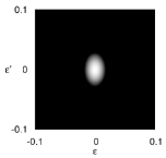
(a) Plain

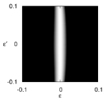
(b) CORPSE

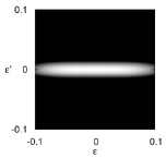
(c) SCROFULOUS

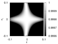
(d) Concatenated pulses

Figure 1: Fidelity ${\cal F}$ of (a) a plain pulse (b) CORPSE ($n_{1}=n_{3}=1,\ n_{2}=2$), (c) SCROFULOUS and (d) the concatenated pulse sequence as a function of the error strength constants $\epsilon$ for the pulse-length error and $\epsilon^{\prime}$ for the off-resonance error. The target unitary operator $U$ is $\exp(-\mathrm{i}\pi\sigma_{2}/2)$. In whiter area the fidelity ${\cal F}$ yields higher value.

For CORPSE, we observe that $T=0$ as expected, since it is designed so as to compensate for the off-resonance error. Further, from Eq. (35), we have $[W^{i},R(m^{j})]=0$, which leads to

$$\Delta W = \epsilon(W^{1}+W^{2}+W^{3})$$

$$= \epsilon\left[\theta/2+(n_{1}-n_{2}+n_{3})\pi\right](\cos\phi\sigma_{1}+\sin\phi\sigma_{2}).$$

Let us choose $\{n_{i}\}$ so that they satisfy

$$n_{1}-n_{2}+n_{3}=0.$$ (45)

Then we have

$$\Delta W = \epsilon m_{\mu}\tau_{\mu},$$ (46)

which is nothing but the pulse-length error acting on the target unitary operator. This clearly tells us that we can compensate for both systematic errors simultaneously, if we use a ConCatenated Composite Pulse (CCCP) sequence of three CORPSE sequences under the condition that they compose the SCROFULOUS when combined together. We call this concatenated pulse by CORPSE In SCROFULOUS-CCCP, or CIS-CCCP for short, in the following.

One could alternatively try a concatenation of three SCROFULOUS pulses under the condition that they compose the CORPSE. This pulse sequence is, however, not robust in the sense of Eq. (3): Each constituent SCROFULOUS in the pulse sequence leads to $S=0$ but $T\neq\sigma_{3}\sin(\theta/2)$. This implies $\Delta W\neq\epsilon^{\prime}U^{{\dagger}}\sigma_{3}\sin(\theta/2)$, that is, in view of the second term in the RHS of Eq. (39), the error which is not compensated for by each SCROFULOUS pulse cannot be regarded as the off-resonance error and the overall CORPSE fails to eliminate it.

We would like to emphasize that the CIS-CCCP sequence cannot be generated by iterative expansions Tycko85 ; Levitt96 . An iterative expansion is composed of consecutive applications of various pulse sequences, each of which is created from a given pulse sequence by i) a permutation and ii) a shift of the rotation axes in the $xy$-plane of constituent pulses. Then, one cannot create a CORPSE with the total rotation angle $\pi$ by operations i) and ii) on a generic CORPSE. This proves impossibility of designing the CIS-CCCP by iterative expansions.

It is of interest to compare the fidelity of CIS-CCCP sequence with those of CORPSE and SCROFULOUS. The fidelity with respect to the target unitary gate $U$ is defined by the absolute value of the Hilbert-Schmidt inner product:

$${\cal F}=\frac{1}{2}\Big{|}\mathrm{Tr}\left[U^{\dagger}R(m^{k}+\delta m^{k})\cdots R(m^{1}+\delta m^{1})\right]\Big{|}.$$ (47)

Note that $k=3$ for CORPSE and SCROFULOUS, whereas $k=9$ for CIS-CCCP.

Our interest lies in the weak error strengths region $-0.1\leq\epsilon,\epsilon^{\prime}\leq 0.1$, since the accuracy threshold theorem requires the error probability less than ${\cal O}(10^{-3})$ for fault tolerant quantum computation Gaitan07 . From Fig. 1, we immediately observe two features of the CIS-CCCP. First, the CIS-CCCP has characteristics of both the SCROFULOUS and the CORPSE pulses, as expected: The CIS-CCCP is robust along the lines $\epsilon\epsilon^{\prime}=0$, whereas the CORPSE is robust along $\epsilon=0$ and the SCROFULOUS along $\epsilon^{\prime}=0$. Second, the whiter area, the higher fidelity region, of the CIS-CCCP is considerably wider than those of the CORPSE and the SCROFULOUS combined together. This observation indicates that the concatenation of composite pulses results in an even more robust pulse sequence.

In closing this section, let us show the difference between the CIS-CCCP and the composite pulse proposed by Alway and Jones Alway07 . Their composite pulse also compensates the pulse-length error and the off-resonance error simultaneously, but implements only $\pi$-pulses along an axis in the $xy$-plane (see Appendix A). Here, we should note that any combinations of $\pi$-pulses along axes on the $xy$-plane are reduced to either $\pi$-pulse on the same plane or the pulse along the $z$-axis:

$$R(m^{k})\cdots R(m^{1})=\begin{cases}R(m),&k=1,3,\dots,\\ R(m^{z}),&k=2,4,\dots.\end{cases}$$ (48)

Here, $m^{j}=\pi(\cos\phi_{j},\sin\phi_{j},0)$ and $m=\pi(\cos\phi,\sin\phi,0)$, where $\phi$ is read as a function of $\{\phi_{j}\}$. We introduced $m^{z}=(0,0,2\Theta)$ with $\Theta=\sum_{j=1}^{k/2}(\phi_{2j}-\phi_{2j-1}+\pi)$. Equation (48) can be derived by mathematical induction with respect to $k$. Therefore, it is impossible to implement arbitrary one-qubit rotations as combinations of their composite pulse sequences. This clearly shows that we cannot realize universal gate set by using their composite pulse sequence. In contrast, the CIS-CCCP does not have such a restriction as Eq. (48), and implements any one-qubit unitary operation by using Euler angles.

IV Conclusion and Discussions

In this paper, we proposed a simple formalism to design unitary gates robust against systematic errors whose magnitude are unknown. By using this method, we systematically derived various criteria which admitted lucid interpretations.

We designed a pulse sequence robust against two types of systematic errors (33) simultaneously. We design a new composite pulse that is the SCROFULOUS out of the CORPSEs in order to take advantages of these composite pulses. Our approach is straightforward than the quaternion algebra that relies on brute force calculation. Our pulse sequence has controllable free parameters; cf. the pulse sequence proposed in Alway07 , which is also robust against the errors (33), but implements only $\pi$-pulse gate on the $xy$-plane. In contrast, our pulse sequence realizes arbitrary one-qubit unitary gate robust against combined errors (33) and will find an important application in implementation of universal gate set out of low quality gates. These features show the usefulness of our formalism as a guiding principle to construct unitary gates robust under coexisting deterministic errors.

We would like to stress that the our scheme is applicable not only to NMR, but also to other physical systems since the condition (9) is formulated independently of the Hamiltonian. For example, the effective Hamiltonian of a quantronium superconducting qubit takes the NMR form Collin04

$$H=-h\nu_{R0}(\cos\xi\sigma_{1}+\sin\xi\sigma_{2})$$ (49)

with an additional off-resonance error term $h\Delta\nu\sigma_{3}$, where $h$ is a constant and $\Delta\nu$ is the detuning. It was demonstrated in Collin04 that CORPSE indeed suppresses the off-resonance error. A similar demonstration of the effectiveness of CORPSE has been made for a neutral atom qubit to suppress effective microwave detuning across the qubit ensemble Rakreungdet09 . Our concatenated composite pulse is applicable to these systems.

Our method is also useful for designing a robust two-qubit gate. Nonetheless, it requires intensive analytical as well as numerical analysis and is beyond the scope of the present paper. Our preliminary result shows that a two-qubit gate with error in the coupling strength between qubits may be made robust against the error by decomposing the gate into a relatively small number of gates, which will be reported elsewhere.

Appendix A Alway and Jones’ gate

In Sec. III, we discussed the composite $\pi$-pulse designed by Alway and Jones Alway07 , which compensates both the pulse-length error and the off-resonance error. Suppose we are to implement a pulse sequence whose rotation axis is in the $xy$-plane. Then the pulse sequence employed in Alway07 is robust under the error (33) if and only if the rotation angle is $\pi$.

The “if” part is proved by Alway and Jones Alway07 as mentioned above. Let us briefly reproduce their result to establish notation and conventions. For notational convenience, we introduce $U(\theta):=\exp\left(-\mathrm{i}\theta\sigma_{1}/2\right)$. (We consider arbitrary rotation axes at the end of Appendix.) Given the target $U(\pi)$, we can design the following pulse sequence:

$$U_{\rm or}U_{\rm pl}U(\pi),$$ (50)

where we introduced two partial sequences

$$U_{\rm pl}=\prod_{i=1}^{3}R(m^{i}),\qquad U_{\rm or}=\prod_{i=4}^{7}R(m^{i}),$$ (51)

whose elementary pulses are given as

$$\theta_{2}=2\pi,\quad\theta_{i}=\pi\quad(i\neq 2)$$

$$\phi_{1}=\phi_{3}=\phi_{\rm pl},\quad\phi_{2}=3\phi_{\rm pl},$$

$$\phi_{4}=2\pi-\phi_{6}=\pi-\phi_{\rm or},\quad\phi_{5}=-\phi_{7}=-\phi_{\rm or},$$ (52)

with $\phi_{\rm pl}=\phi_{\rm or}=\arccos(-1/4)$. $U_{\rm pl}U(\pi)$ is a composite pulse known as BB1 Wimperis , which is robust against the pulse-length error, while $U_{\rm or}U(\pi)$ is a composite pulse robust against the off-resonance error. Note that

$$U_{\rm pl}=U_{\rm or}=\openone$$ (53)

in the absence of errors. This is the sequence proposed in Alway07 .

Now let us prove the “only if” part. Suppose we want to implement $U(\theta)$, which is robust against simultaneous errors by employing the sequence (50). Here we assume $\theta$ is not fixed to $\pi$ and $\phi_{\rm pl}$ and $\phi_{\rm or}$ are adjusted so as to make the gate robust for a given $\theta$. After simple calculation, we obtain the zeroth and the first order error terms as

$$U(\theta)-\mathrm{i}\epsilon\frac{\theta}{2}\sigma_{1}U(\theta)-\mathrm{i}\epsilon^{\prime}\sin\frac{\theta}{2}\sigma_{3},$$ (54)

for the target $U(\theta)$. In the same way, we have

$$U_{\rm pl}=\openone-2\pi\mathrm{i}\epsilon\cos\phi_{\rm pl}\sigma_{1}$$ (55)

and

$$U_{\rm or}=\openone+4\mathrm{i}\epsilon^{\prime}\cos\phi_{\rm or}\sigma_{2}.$$ (56)

Taking product of (54), (55) and (56) and evaluating the coefficients of $\epsilon$ and $\epsilon^{\prime}$, we find that this composite pulse is robust against the simultaneous errors only if $\theta$, $\phi_{\rm pl}$ and $\phi_{\rm or}$ satisfy the conditions:

$$2\pi\cos\phi_{\rm pl}+\frac{\theta}{2}=0,\quad 4\cos\phi_{\rm or}\sigma_{2}U(\theta)-\sin\frac{\theta}{2}\sigma_{3}=0.$$ (57)

These conditions have a unique nontrivial solution

$$\phi_{\rm pl}=\phi_{\rm or}=\arccos(-1/4),\quad\theta=\pi,$$ (58)

which shows that the rotation angle of the target pulse must be $\pi$.

Clearly the rotation axis can be any direction in the $xy$-plane by a simple redefinition of the coordinate axes or by applying the similarity transformations around the $z$-axis to each constituent pulses. This completes the proof of the “only if” part.

References

- (1) M. A. Nielsen and I. C. Chuang, Quantum Information and Quantum Computation, (Cambridge University Press, Cambridge, 2000).
- (2) M. Nakahara and T. Ohmi Quantum Computing: From Linear Algebra to Physical Realizations, (Taylor and Francis, Boca Raton, 2008).
- (3) F. Gaitan, Quantum Error Correction and Fault Tolerant Quantum Computing, (Taylor and Francis, Boca Raton, 2008).
- (4) P. Zanardi and M. Rasetti, Phys. Lett. A 264, 94 (1999).
- (5) S.-L. Zhu and Z. D. Wang, Phys. Rev. Lett. 89, 097902 (2002).
- (6) A. Blais and A.-M. S. Tremblay, Phys. Rev. A 67, 012308 (2003).
- (7) S.-L. Zhu and P. Zanardi, Phys. Rev. A 72, 020301(R) (2005).
- (8) Y. Ota, Y. Goto, Y. Kondo and M. Nakahara, Phys. Rev. A 80, 052311 (2009).
- (9) Y. Kondo and M. Bando, J. Phys. Soc. Jpn. 80, 054002 (2011).
- (10) S.-L. Zhu and Z. D. Wang, Phys. Rev. A 67, 022319 (2003).
- (11) P. Solinas, P. Zanardi, N. Zanghí and F. Rossi, Phys. Rev. A 67, 052309 (2003).
- (12) Y. Ota, M. Bando, Y. Kondo and M. Nakahara, Phys. Rev. A 78, 052315 (2008).
- (13) M. V. Berry, Proc. R. Soc. Lond. A 392, 45 (1984).
- (14) F. Wilczek and A. Zee, Phys. Rev. Lett. 52, 2111 (1984).
- (15) Y. Aharonov and J. Anandan, Phys. Rev. Lett. 58, 1593 (1987).
- (16) D. N. Page, Phys. Rev. A 36, 3479 (1987).
- (17) J. Anandan, Phys. Lett. A 133, 171 (1988).
- (18) A. Shapere and F. Wilczek, Geometric Phases in Physics, (World Scientific, Singapore, 1989).
- (19) M. Nakahara, Geometry, Topology and Physics (2nd ed.) (Taylor and Francis, Boca Raton, 2003).
- (20) C. A. Mead, Rev. Mod. Phys. 64, 51 (1992).
- (21) Y. Ota and Y. Kondo, Phys. Rev. A 80, 024302 (2009).
- (22) M. H. Levitt and R. Freeman, J. Magn. Reson. 43, 502 (1981).
- (23) C. Counsell, M. H. Levitt and R. R. Ernst, J. Magn. Reson. 63, 133 (1985).
- (24) R. Tycko, A. Pines and J. Guckenheimer, J. Chem. Phys. 83, 2775 (1985).
- (25) A. J. Shaka and A. Pines, J. Magn. Reson. 71, 495 (1987).
- (26) M. H. Levitt, in Encyclopedia of Nuclear Magnetic Resonance, edited by D. M. Grant and R. K. Harris (Wiley, 1996), p.1396.
- (27) R. Freeman, Spin Choreography, (Oxford University Press, Oxford, 1999).
- (28) T. D. W. Claridge, High-Resolution NMR Techniques in Organic Chemistry, (Elsevier, Oxford, 1999).
- (29) H. K. Cummins and J. A. Jones, New J. Phys. 2, 6 (2000).
- (30) H. K. Cummins, G. Llewellyn and J. A. Jones, Phys. Rev. A 67, 042308 (2003).
- (31) M. Möttönen, R. de Sousa, J. Zhang and K. B. Whaley, Phys. Rev. A 73, 022332 (2006).
- (32) W. G. Alway and J. A. Jones, J. Magn. Reson. 189, 114 (2007).
- (33) R. Tycko, H. M. Cho, E. Schneider and A. Pines, J. Magn. Reson. 61, 90 (1985).
- (34) E. Collin, G. Ithier, A. Aassime, P. Joyez, D. Vion and D. Esteve, Phys. Rev. Lett. 93, 157005 (2004).
- (35) W. Rakreungdet, J. H. Lee, K. F. Lee, B. E. Mischuck, E. Montano, and P. S. Jessen, Phys. Rev. A 79, 022316 (2009).
- (36) S. Wimperis, J. Magn. Reson. A 109, 221 (1994).