Quantum Spin Hall Effect in Graphene Nanoribbons: Effect of Edge Geometry

Abstract

There has been tremendous recent progress in realizing topological insulator initiated by the proposal of Kane and Mele for the graphene system. They have suggested that the odd $Z_{2}$ index for the graphene manifests the spin filtered edge states for the graphene nanoribbons, which lead to the quantum spin Hall effect(QSHE). Here we investigate the role of the spin-orbit interaction both for the zigzag and armchair nanoribbons with special care in the edge geometry. For the pristine zigzag nanoribbons, we have shown that one of the $\sigma$ edge bands located near $E=0$ lifts up the energy of the spin filtered chiral edge states at the zone boundary by warping the $\pi$-edge bands, and hence the QSHE does not occur. Upon increasing the carrier density above a certain critical value, the spin filtered edge states are formed leading to the QSHE. We suggest that the hydrogen passivation on the edge can recover the original feature of the QSHE. For the armchair nanoribbon, the QSHE is shown to be stable. We have also derived the real space effective hamiltonian, which demonstrates that the on-site energy and the effective spin orbit coupling strength are strongly enhanced near the ribbon edges. We have shown that the steep rise of the confinement potential thus obtained is responsible for the warping of the $\pi$-edge bands.

I Introduction

Recently, the role of intrinsic spin-orbit coupling(SOC) in graphene and graphene multilayer systems has attracted a lot of attention as one of the model system to realize the new quantum state of matter and also for the possible spintronics applicationa1 ; a2 ; a3 ; a4 ; a5 ; a6 ; a7 ; a8 ; a9 ; a10 ; a11 ; a12 ; a13 ; a14 ; a15 ; a16 ; a17 ; a18 ; a19 ; a20 ; a21 ; a22 ; a23 ; a24 ; a25 ; a26 . It has been well known that upon including the SOC, graphene supports the quantum spin Hall effect(QSHE). This implies that there exist spin filtered chiral states at the edges of graphene leading to the nonzero quantized spin currenta1 ; a2 ; a3 . It has been argued that the odd $Z_{2}$ index of the bulk graphene guarantees the existence of the QSHEa1 ; a10 ; a16 ; a27 ; a28 . This integral number represents the inherent topological properties of graphene just as the Chern number characterizes the quantum Hall systemsa29 ; a30 . Furthermore this interesting role of the SOC in graphene has stimulated the studies on the novel kind of material called the topological insulator(TI)t1 ; t2 ; t3 ; t4 . Following the initial theoretical proposal to graphene, several other materials have been theoretically suggested to be possible candidates of TI, which have been experimentally confirmed later ont2 ; t3 . In contrast, the QSHE of graphene has not been experimentally observed yet. This may be due to the weak intrinsic SOC in graphene so that the energy dispersion of the edge state is too small to be resolved at experimentally feasible temperature scalea5 ; a6 ; a7 . More interestingly, one can speculate that the graphene nanoribbon system may demonstrate the unexpected interplay between the topological properties based on the bulk energy band and the edge geometry of the nanoribbon. In this regard, the graphene nanoribon system will serve as a standard model whose edge geometry can be well characterized and controlled by a few parametersa10 .

The existence of the QSHE in graphene as mentioned above is mostly based on the study of the Kane-Mele(KM) model which has received considerable attention as a realization of the Haldane’s original idea about the quantum Hall effect without magnetic field in the honeycomb latticehaldane . In the KM-hamiltonian, the low energy processes between $p_{z}$ orbitals mediated by the SOC are described by the imaginary next nearest neighbor(n.n.n.) hopping terms $i\xi_{1}/3\sqrt{3}\nu_{ij}s^{z}_{\alpha\beta}c^{\dagger}_{i\alpha}c_{j\beta}$a1 ; a2 . Based on the group theoretical and perturbative arguments, it has been elucidated that the SOC term for the nearest neighbor(n.n.) hopping process vanishes at the Dirac point by the lattice symmetry of graphene and hence the leading SOC term originates from the n.n.n. hopping processesa5 ; a6 ; nnn1 . Several authors have indicated that one can obtain much more enhanced intrinsic spin orbit coupling(ISOC) such as the new hopping processes in the bilayer graphene system, which arise due to the different lattice symmetries around each carbon atomb1 ; b2 . Here we want to emphasize that in the graphene nanoribbons, one should be very careful in applying the low-energy effective hamiltonian to the edges of the graphene, where the bulk lattice symmetry is broken.

In the paper, we investigate the effect of the edge geometry on the low energy physics of the intrinsic SOC both in the zigzag and armchair nanoribbons based on the tight binding hamiltonian. In order to describe the SOC, we have included the $s,p_{x},p_{y}$ and $p_{z}$ orbitals of carbon atoms instead of using the effective Kane-Mele term containing the $p_{z}$ orbital alone. For the pristine zigzag nanoribbon, we have demonstrated that one of the $\sigma$ edge bands made of the $s,p_{x},p_{y}$ orbitals located near $E=0$ lifts up the energy of the spin filtered chiral edge states at the zone boundary, and hence the QSHE does not occur. By increasing the carrier density within a certain range, the system exhibits the QSHE with spin filtered chiral edge states. By further increasing the carrier density above a certain critical value, the QSHE disappears again by adding an extra pair of edge states leading to the even number of edge states at each side of the edges. We have also studied the role of hydrogen passivation on the edges, whose orbitals hybridize with the $\sigma$ edge bands located near $E=0$ and then the two edge bands are repelled from each other by creating large energy gaps. Remarkably, we have noticed that the original feature of the QSHE revives with hydrogen passivation. For the armchair graphene nanoribbon(AGNR), we have noticed that the QSHE is mostly quite stable with or without passivation. However the edge state of the armchair nanoribbon is too widely spread from the edge on the order of $(\gamma_{0}/\xi_{1})a\cong 1mm$, where $\gamma_{0}$ represents the nearest neighbor hopping amplitude of the $\pi$ electrons, $\xi_{1}$ the SOC induced next nearest neighbor hopping amplitude, and $a$ the lattice spacing.

In the section II, we have introduced the tight binding hamiltonian, which describes the graphene nanorribbon system. The hamiltonian includes both the $p_{z}$ and the $s,p_{x},p_{y}$ orbitals of carbon atom, the atomic spin-orbit coupling term, and the edge passivation term. In the section III, we have investigated the band structure of the pristine ZGNR and then the band structure of the AGNR is subsequently calculated. In the section IV, the effect of hydrogen passivation on the band structure of the ZGNR is studied. In the section V, we have constructed the real space effective hamiltonian for the ZGNR. The summary will follow in the section VI.

II The tight binding hamiltonian

The $\pi$ and $\sigma$ bands of the ZGNR can be obtained by the following tight binding hamiltonian

$$H=H_{\pi}+H_{\sigma}+H_{SO}$$ (1)

where $H_{\pi}$ represents the nearest neighbor hopping processes between $p_{z}$ orbitals, $H_{\sigma}$ the matrix elements among $s$, $p_{x}$, and $p_{y}$ orbitals, $H_{SO}$ the on-site atomic spin orbit coupling term which connects the two Hilbert spaces together. The hamiltonian $H_{\pi}$ for the $p_{z}$ orbitals of the ZGNR is given as followsneto

$$H_{\pi}=\gamma_{0}\sum_{\langle i,j,m,n\rangle}[C^{\dagger}_{p_{z},B,j,n}C_{p_{z},A,i,m}+\mathrm{h.c.}],$$ (2)

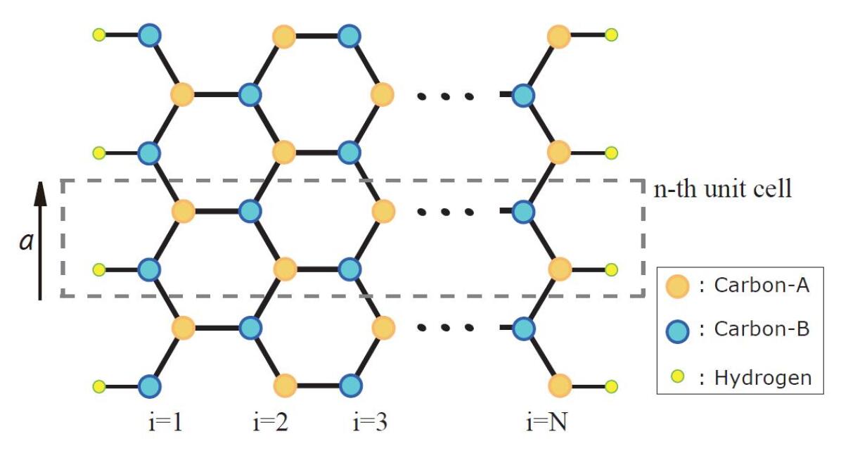
Figure 1: (Color online) Hydrogen passivated ZGNR with width N. Two sublattices of the honeycomb lattice are represented by ‘carbon-A’ and ‘carbon B’.

where the indices $A(B)$, $i$($j$) and $m$($n$) represent the sublattices, dimer lines, and unit cells along the $y$-direction respectively as shown in Fig. 1 and $\gamma_{0}=V_{pp\pi}=-3.03\mathrm{eV}$. The angular bracket under the summation stands for the nearest neighbor pairs. The hamiltonian $H_{\sigma}$ can be written by

$$H_{\sigma}=\sum_{\alpha,i,m}\mathbb{C}^{\dagger}_{\alpha,i,m}\mathbb{E}_{0}\mathbb{C}_{\alpha,i,m}+\sum_{\langle i,j,m,n\rangle}[\mathbb{C}^{\dagger}_{B,j,n}\mathbf{\Sigma}_{l}\mathbb{C}_{A,i,m}+\mathrm{h.c.}]$$ (3)

where the index $\alpha$ represents the sublattices $A,B$. The on-site spin-orbit coupling term is given by $H_{SO}=\frac{\xi_{0}}{2}\sum\vec{L}\cdot\vec{s}$. We have omitted the summation over the spin indices in $H_{\sigma}$, since the hamiltonian is invariant over spin. $\mathbb{C}_{\alpha,i,m}$ is a column vector of a form $[c_{p_{y}}~{}c_{p_{x}}~{}c_{s}]^{\mathrm{T}}$ at each site $\{\alpha,i,n\}$, while $\mathbb{E}_{0}$ and $\mathbf{\Sigma}_{l}$ represent the on-site and hopping matrices respectively with $l=(1+i-j)(m-n+\frac{3-(-1)^{i}}{2})$, which have the following matrix elements for the case of zigzag termination

$$\mathbb{E}_{0}=\left(\begin{array}[]{ccc}0{}&0{}&0\\ 0{}&0{}&0\\ 0{}&0{}&\epsilon_{s}\end{array}\right)$$ (7)

$$\mathbf{\Sigma}_{0}=\left(\begin{array}[]{ccc}V_{pp\pi}&0&0\\ 0&-V_{pp\sigma}&V_{sp\sigma}\\ 0&-V_{sp\sigma}&V_{ss\sigma}\end{array}\right)$$ (11)

$$\mathbf{\Sigma}_{1}=\left(\begin{array}[]{ccc}(V_{pp\pi}-3V_{pp\sigma})/4&\sqrt{3}(V_{pp\pi}+V_{pp\sigma})/3&\sqrt{3}V_{sp\sigma}/2\\ \sqrt{3}(V_{pp\pi}+V_{pp\sigma})/3&(3V_{pp\pi}-V_{pp\sigma})/4&-V_{sp\sigma}/2\\ -\sqrt{3}V_{sp\sigma}/2&V_{sp\sigma}/2&V_{ss\sigma}\end{array}\right)$$ (15)

$$\mathbf{\Sigma}_{2}=\left(\begin{array}[]{ccc}(V_{pp\pi}-3V_{pp\sigma})/4&-\sqrt{3}(V_{pp\pi}+V_{pp\sigma})/3&-\sqrt{3}V_{sp\sigma}/2\\ -\sqrt{3}(V_{pp\pi}+V_{pp\sigma})/3&(3V_{pp\pi}-V_{pp\sigma})/4&-V_{sp\sigma}/2\\ \sqrt{3}V_{sp\sigma}/2&V_{sp\sigma}/2&V_{ss\sigma}\end{array}\right).$$ (19)

Here, $\epsilon_{s}=-8.87\mathrm{eV}$ is the on-site energy of the $s$ orbital relative to that of the $p$ orbital and the various hopping parameters are chosen to be $V_{pp\pi}=-3.03,V_{pp\sigma}=-5.04,V_{sp\sigma}=-5.58$ and $V_{ss\sigma}=-6.77$ in eVsaito . In the bulk two dimensional case, one can obtain the intrinsic spin orbit interaction strength $\xi_{1}\approx 2\xi_{0}^{2}\epsilon_{s}/9V_{sp\sigma}^{2}\sim 10^{-3}\mathrm{meV}$ at Dirac points using the above parameters with $\xi_{0}\approx 4$meVa7 . We will also include the hamiltonian $H_{\mathrm{P}}$ to take into account the passivation of the dangling orbitals at the edges of the graphene nanoribbon. The specific form of $H_{\mathrm{P}}$ will be given in the section IV. For the pristine graphene nanoribbons, that is, the non-passivated ZGNR in which the dangling bonds at the edges are kept intact, we will apply the open boundary condition. Other extrinsic spin orbit coupling terms such as the Rashba interaction are not considered here.

III The pristine zigzag graphene nanoribbon

The effects of the spin orbit coupling on the electronic properties of the Dirac particles in graphene have been extensively studied recentlya1 ; a2 ; a5 ; a6 ; a7 ; a9 . Since the energy levels of $\sigma$ bands are well separated from the Dirac points, one can obtain the low-energy effective hamiltonian projected to the Hilbert space of the $p_{z}$ orbital alone by integrating out the high energy processes involving the $\sigma$ bandspert : $H_{\mathrm{eff}}\simeq H_{\pi}-H_{SO}H_{\sigma}^{-1}H_{SO}$. It has been shown that the nearest neighbor (n.n.) hopping amplitude induced by the SOC is cancelled by the lattice symmetry and thus the leading contribution due to the intrinsic SOC results from the effective next nearest neighbor (n.n.n.) hopping processes of the following form $i\xi_{1}/3\sqrt{3}(\vec{d}_{ik}\times\vec{d}_{kj})c^{\dagger}_{i}s^{z}c_{j}$a1 ; a2 , where $\xi_{1}$ is on the order of 0.05Ka5 ; a7 . This effective hamiltonian, so called the KM hamiltonian, has been generally used to study the edge states of graphene nanoribbon, which led to the QSHE. However, we want to point out that since the lattice symmetry is broken at the graphene edges, one should in principle use the full hamiltonian instead of the truncated low-energy effective KM hamiltonian. In doing so, it is generally observed that the characteristic behavior of the QSHE in the ZGNR depends largely on the edge geometry and the passivation.

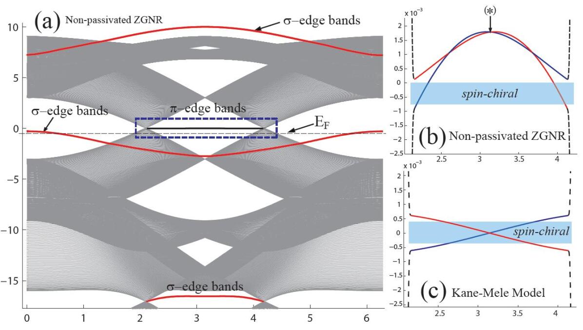
Figure 2: (Color online) (a) Band structure of the pristine ZGNR with width $N=150$ and the atomic SOC strength $\xi_{0}=0.1\mathrm{eV}$. Here the $x$-axis represents the dimensionless wave number $ka$ and the $y$-axis the energy in eV. The red curves represent the $\sigma$ edge bands made of $s,p_{x},p_{y}$ orbitals. In the blue dashed box at the band center, we have the $\pi$ edge bands which look almost flat at this energy scale. (b) The dashed box in Fig. 2(a) is magnified. (c) The band structure near the band center obtained by Kane-Mele model with $\xi_{1}=6.34\times 10^{-4}\mathrm{eV}$. In (b) and (c), the red(blue) bands include edge states confined to the right(left) side of the ribbon.

In Fig. 2(a), we have shown the calculated band structure of the pristine ZGNR with width $N=150$. From the two degenerate uncoupled compositions of the spin and orbit $\{p_{z}\uparrow,p_{x}\downarrow,p_{y}\downarrow,s\downarrow\}$ and $\{p_{z}\downarrow,p_{x}\uparrow,p_{y}\uparrow,s\uparrow\}$, we have plotted the former one in Fig. 2(a). Here, we have taken a relatively large value of the SOC $\xi_{0}=0.1$eV for the sake of clarity, since we have noticed that the magnitude of the SOC hardly affects the qualitative features of the band structures. In order to investigate the edge states made of the $p_{z}$ orbital in detail, we focus on the $\pi$-edge bands within the dashed box of Fig. 2(a), which are magnified in Fig. 2(b). We have also calculated the band structure based on the effective KM hamiltonian, which is shown in Fig. 2(c) and compared to the result from our model. We have chosen $\xi_{1}\approx 2\xi_{0}^{2}\epsilon_{s}/9V_{sp\sigma}^{2}=6.34\times 10^{-4}$eV for the KM-hamiltonian, which corresponds to $\xi_{0}=0.1$eV for our hamiltonian.

By the simple band counting, one can expect to have $(2N-2)\times 4$ bulk bands and the $2\times 4=8$ edge bands composed of the four atomic orbitals, all of which are two-fold spin degenerate due to the time reversal and the inversion symmetry. The most part of the band structure can be understood as a confinement effect on the bulk two dimensional graphene. The almost flat bands within the black dashed box and the red bands are the newly introduced states which are absent in the bulk graphene. They represent the edge localized states, where the former ones ($\pi$ edge bands) are mostly made of $p_{z}$ orbital and the latter ones ($\sigma$ edge bands) mainly consists of $s,p_{x},p_{y}$ orbitals. These features of the band structures of the ZGNR are consistent with the previous first principles calculationscho . It has also been widely known that the gapless flat bands of $p_{z}$ orbital are formed at $E=0$ within the finite region of $2\pi/3<k<\pi$ in the absence of the SOC. It is shown in Fig. 2(a) that there exist six $\sigma$ edge bands with two-fold spin degeneracy and three pairs of them are almost degenerate so that it seems only three $\sigma$ bands exist. For the stronger SOC, they will split into distinct six non-degenerate bands. While two pairs of them are well separated from the $\pi$ edge bands, a pair of the $\sigma$ edge bands appear quite close to the $\pi$ edge ones. Since two pairs of edge $\sigma$ bands lie below the $\pi$ edge bands, the Fermi level of the undoped ZGNR is located below the $\pi$ edge ones as shown in Fig. 2(a).

At this charge neutral point, we have the edge localized states coming from the two $\sigma$ edge bands, which become degenerate at the zone boundary. At a fixed value of $k$ away from the zone boundary, the two almost degenerate $\sigma$ bands are shown to be localized at different edges leading to the even number of pairs of edge states at each edge. Hence the QSHE does not occur. In contrast to our results, the KM-model exhibits the spin filtered edge states within the energy window of width $2\xi_{1}$ around the band crossing point at the zone boundary and thus one can expect the QSHE to occur as shown in Fig. 2(c).

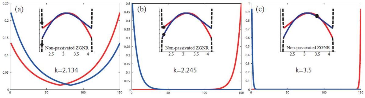
Figure 3: Eigenvectors of the $\pi$ edge states at several values of $k$. The x-axis represents the index of the dimer lines of the ribbon and the y-axis the absolute value of the amplitude of the eigenvector at each dimer line. (a) The eigenvector at $k=2.134$, (b) the eigenvector at $k=2.245$, and (c) the eigenvector at $k=3.5$. The blue(red) colored eigenvectors correspond to the blue(red) bands. Here, the blue(red) bands consist of the edge states localized at the left(right) side.

The $\pi$-edge bands are shown in Fig. 2(b) and 2(c), where the red and blue bands consist of the edge states confined to the right and left edge of the ribbon respectively. The black dashed bands represent the states, whose amplitudes are spread over both edges. For another set of the spin-orbit composition $\{p_{z}\downarrow,p_{x}\uparrow,p_{y}\uparrow,s\uparrow\}$, one can simply interchange the red and blue colors of the bands. In Fig. (3), we have shown that the states within the $\pi$-edge bands ($k=2.245,3.5$) are strongly confined to one of the ribbon edges with the localization length $\xi\cong a/\ln(-2\cos ka/2)$, which vanishes as $k$ approaches to the zone boundary ($k=\pi$). In contrast, the states at $k=2.134$ have a bulk feature, which have finite amplitudes along the width direction.

By increasing the carrier density, one can adjust the Fermi energy into the region, where spin filtered chiral edge states made of the $\pi$ orbitals do exist within the energy window of width $2\xi_{1}$ and the QSHE will appear. Here the red and blue bands are monotonic and move in the opposite directions to each other. With a further increase of the carrier density, one can raise the Fermi energy to the band crossing point at the zone boundary. At this time reversal invariant point denoted by an asterisk in Fig. 2(b), the edges states are most strongly confined to the ribbon edges for both the KM model and ours. While the KM model yields the QSHE near this point with a single pair of edge states at each edge as shown in Fig. 2(c), our model demonstrates that two chiral spin bands are non-monotonic and they cross the Fermi level several times as shown in Fig. 2(b). There exist edge states propagating in both directions at each edge of the ribbon. Although the number of bands crossing the Fermi level is odd, one of them(black dashed one) is always dispersed at both edges manifesting the feature of quantum confined bulk band. This means that there exist two pairs of edge states at each edge and hence the QSHE is not feasible in this energy range.

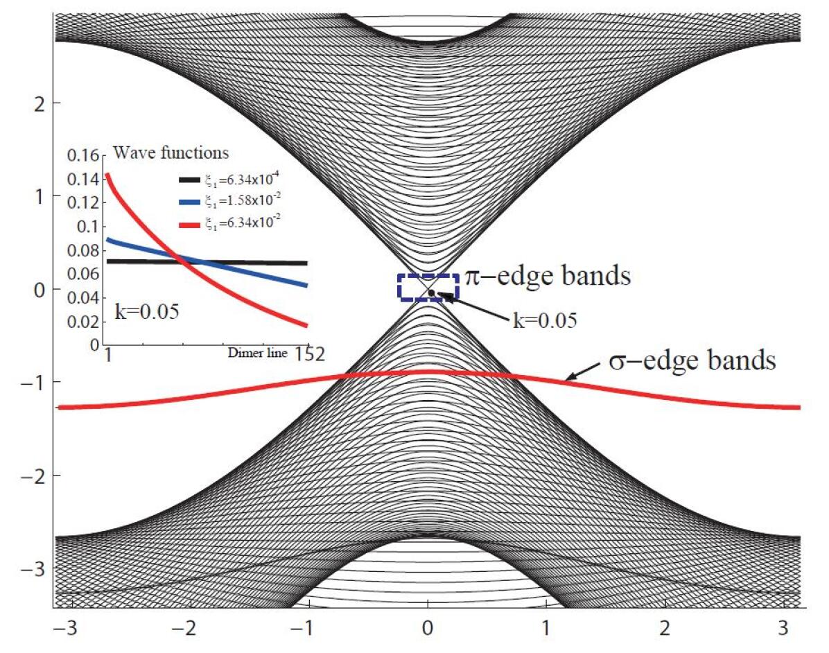
Figure 4: (Color online) Band structure of the non-passivated AGNR with width $N=152$. The red bands represent the $\sigma$ edge bands which are almost doubly degenerate. Within the dashed box, we have the edge localized $\pi$ bands. In the inset, the amplitudes for the eigenvectors at $k=0.05$ are plotted as a function of dimer line index for three different values of $\xi_{1}=6.34\times 10^{-4},1.58\times 10^{-2},6.34\times 10^{-2}$ in eV. One can notice that the edge states are quite broadly dispersed rather than localized to the edge.

We have also studied the effect of the spin orbit coupling on the band structure of the AGNR. In comparison to the ZGNR, the Dirac cone is located at the $\Gamma$ point ($k=0$), which becomes split in energy upon the inclusion of the SOC. It is well known that in the absence of the SOC, the gapless edge bands exist which crosses $E=0$ at $k=0$ for $N+1$ being an integer multiple of three. Hence the main difference between the ZGNR and the AGNR lies in the fact that while there exist a finite range of gapless flat bands for the ZGNR, there is a single gapless point at $k=0$. In Fig. 4, the band structure of the AGNR with width $N=152$ is plotted. One can clearly see that the $\pi$ edge bands are formed around $k=0$ within the energy range of $2\xi_{1}$ and hence the QSHE is expected to occur. The amplitudes of the eigenvectors at a fixed value of $k=0.05$ are plotted as a function of dimer line index for three different values of $\xi_{1}=6.34\times 10^{-4},1.58\times 10^{-2},6.34\times 10^{-2}$ in eV. One can notice that in contrast to the case of ZGNR, the $\pi$ edge states for the AGNR are quite widely spread. The localization length of the edge states for the AGNR can be approximately given by $(\gamma_{0}/\xi_{1})a$ with $a$ being the lattice spacing.

IV The hydrogen passivated zigzag graphene nanoribbon

In the section, we will investigate the effect of the hydrogen passivation on the edge dangling bonds of the ZGNR. Since the hydrogen atom has a single $s$ orbital, only the $p_{x}$ and $s$ orbitals of the adjacent carbon atom will have a finite overlap with the hydrogen atom so that the hamiltonian $H_{\mathrm{P}}$ for the edge passivation can be written as follows

$$H_{\mathrm{P}} = \sum_{n}\Big{[}\tilde{V}_{sp}c^{\dagger}_{p_{x},A,N,n}h_{N,n}+\tilde{V}_{ss}c^{\dagger}_{s,A,N,n}h_{N,n}-\tilde{V}_{sp}c^{\dagger}_{p_{x},B,1,n}h_{1,n}+\tilde{V}_{ss}c^{\dagger}_{s,B,1,n}h_{1,n}+\mathrm{h.c.}\Big{]}$$ (20)

$$+\sum_{n}\varepsilon_{h}(h^{\dagger}_{1,n}h_{1,n}+h^{\dagger}_{N,n}h_{N,n}),$$

where the two hopping and on-site parameters between the carbon and hydrogen atom are taken to be $\tilde{V}_{sp}=-4.5$, $\tilde{V}_{ss}=-4.2$ and $\varepsilon_{h}=-2.7$ in eVpoly . The operator $h^{\dagger}_{i,n}$($h_{i,n}$) represents the creation(annihilation) operator of an electron at hydrogen atom bonded to the $i$-th carbon dimer line in the $n$-th unit cell.

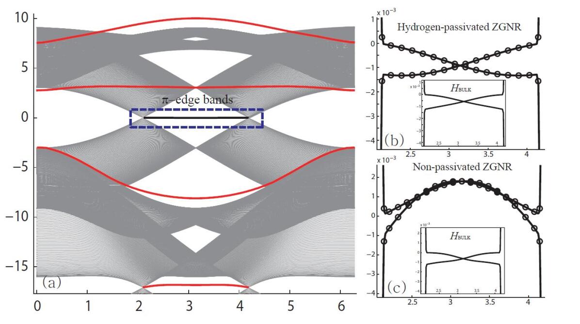
Figure 5: (Color online) Band structure of the ZGNR with width $N=150$ (a) with hydrogen passivation. The passivation parameters are taken to be $\tilde{V}_{sp}=-4.5$, $\tilde{V}_{ss}=-4.2$ and $\varepsilon_{h}=-2.7$ in eV. The red bands represent the $\sigma$-edge states. (b) The solid lines represent the magnified view of the $\pi$ edge bands in the blue dashed box. The open circles correspond to the result obtained from the perturbation method. (c) The solid lines represent the $\pi$ edge bands without passivation. The open circles correspond to the result obtained from the perturbation method for the non-passivated ZGNR. The insets of (b), (c) stand for the results obtained from $H_{\mathrm{bulk}}$.

The band structure of the hydrogen passivated ZGNR is shown in Fig. 5(a). There exist eight $\sigma$-edge bands(red ones) which are composed of four pairs of almost doubly degenerate bands. In comparison to the non-passivated ZGNR, we have an additional pair of $\sigma$ edge bands, since the hydrogen $s$-orbitals at both edges have been coupled to the original $s$ and $p_{x}$ orbitals in the edge carbon atoms. Since the on-site energy $\varepsilon_{h}=-2.7\mathrm{eV}$ of hydrogen atom is quite close to the band bottom of the $\sigma$ edge band located in the middle for the non-passivated ZGNR, they strongly interact with each other and then repel as shown in Fig. 5(a). This makes two significant effects on the edge state characteristics. Focusing on the $\pi$-edge bands shown in Fig. 5(b), one can notice that the general feature of the KM-model is recovered upon hydrogen passivation. In addition, a newly introduced pair of $\sigma$ edge bands are placed above the $\pi$ edge bands. This balances the number of energy bands above and below the $\pi$ edge bands so that the Fermi level at half filling is placed on the $\pi$ edge bands.

By comparing the positions of the $\sigma$ edge bands in Fig. 2(a) and 5(a), one may presume that the $\sigma$-edge bands located close to $E=0$ mainly affect the energy dispersion of the $\pi$-edge band. In order to confirm this scenario, we have studied the effects of the $\sigma$-edge bands by using the perturbation method, where the low-energy effective hamiltonian is given by $H_{\mathrm{eff}}\simeq H_{\pi}-H_{SO}H_{\sigma}^{-1}H_{SO}$. The hamiltonian $H_{\mathrm{eff}}$ can be decomposed into two terms: $H_{\mathrm{eff}}=H_{\mathrm{bulk}}+H_{\mathrm{edge}}$, where $H_{\mathrm{bulk}}$ and $H_{\mathrm{edge}}$ for a given $k$ can be written by

$$H_{\mathrm{bulk}}=H_{\pi}-\sum_{i\in\mathrm{bulk}}H_{SO}|v_{\sigma i}\rangle E_{\sigma i}^{-1}(k)\langle v_{\sigma i}|H_{SO}$$

$$H_{\mathrm{edge}}=-\sum_{i\in\mathrm{edge}}H_{SO}|v_{\sigma i}\rangle E_{\sigma i}^{-1}(k)\langle v_{\sigma i}|H_{SO}.$$ (21)

Here $|v_{\sigma i}\rangle$ represents the eigenstate of the hamiltonian ${\tilde{H}}_{\sigma}=H_{\sigma}+H_{\mathrm{P}}$ in the $i$-th $\sigma$ band and $\sum_{i\in\mathrm{bulk}}$($\sum_{i\in\mathrm{edge}}$) stands for the sum over the bulk(edge) eigenstates. We expect that $H_{\mathrm{bulk}}$ will reproduce the Kane-Mele hamiltonian and thus will always produce spin chiral edge bands at the band center, which is clearly demonstrated in the insets of both Fig. 5(b) and 5(c).

By including the $\sigma$ edge band contribution $H_{\mathrm{edge}}$ to $H_{\mathrm{bulk}}$, we have obtained the results denoted by the open circles in Fig. 5(b) and 5(c). The solid lines represent the exact numerical results of the full hamiltonian, which give an excellent agreement with those from the perturbation method. Hence we have clearly demonstrated that the hydrogen passivation can change the general features of the $\pi$-edge band by modifying the $\sigma$-edge band profile.

V The effective real space hamiltonian for the ZGNR

In the previous section, we have obtained an effective hamiltonian $\textrm{H}_{\textrm{eff}}(k)$ projected to the Hilbert space spanned by the $p_{z}$ orbitals in the momentum space using the perturbaion method. Here we will obtain the real space effective hamiltonian by applying the inverse Fourier transformation(IFT) to $\textrm{H}_{\textrm{eff}}(k)$ and analyze the the spatial dependence of the on-site energy and hopping parameters. For instance, if one applies the IFT to the $\textrm{H}_{\textrm{eff}}(\vec{k})$ of the two dimensional graphene including the SOC term, one can obtain the n.n.n. hopping terms as a leading imaginary hopping process in addition to the original Dirac hamiltonian leading to the KM-hamiltonian written by $\textrm{H}_{\textrm{KM}}=\gamma_{0}\sum_{\langle ij\rangle}c^{\dagger}_{i\alpha}c_{j\alpha}+\sum_{\langle\langle ij\rangle\rangle}i\xi_{1}/3\sqrt{3}\nu_{ij}s^{z}_{\alpha\beta}c^{\dagger}_{i\alpha}c_{j\beta}$.

By investigating the real space hamiltonian for the ZGNR, we have been able to study the effect of the broken translation symmetry at the ribbon edges and the hydrogen passivation as well. The IFTs of the $\textrm{H}_{\textrm{eff}}(k)$ for both the non-passivated and hydrogen passivated ZGNR have yielded as the leading orders the spatially dependent on-site potential and the imaginary n.n.n. hopping amplitude as shown in Fig. 6(a)-(d). We have also checked the additional n.n. hopping term induced by the SOC, which is absent in the 2D graphene due to the bulk lattice symmetry. We note that it is finite but much smaller than that of the n.n.n. hopping processes at the edges and exponentially decreases away from the edges approaching to zero which is its asymptotic limit. Based on the above parameters, we have constructed the following real space effective hamiltonian to describe the ZGNR

$$\textrm{H}_{\textrm{eff}}=\gamma_{0}\sum_{\textrm{n.n.}}c^{\dagger}_{\alpha,i,n}c_{\beta,j,m}+i\sum_{\textrm{n.n.n.}}\xi_{1}(j)/3\sqrt{3}\nu_{in,jm}c^{\dagger}_{\alpha,i,n}c_{\alpha,j,m}+\sum_{\alpha,i,n}E_{0}(i)c^{\dagger}_{\alpha,i,n}c_{\alpha,i,m}$$ (22)

where the indices $\alpha(\beta)$, $i(j)$ and $m(n)$ stand for sublattices, dimer lines and unit cells along the longitudinal direction respectively. The first term represents the non-interacting Dirac hamiltonian and $\xi_{1}(i)$ and $E_{0}(i)$ stand for the imaginary n.n.n. hopping amplitude and the on-site potential energy, which depend on the dimer line index. In Fig. 6(a)-(d), we plot $E_{0}(i)$ and $\tilde{\xi}_{1}(i)=\xi_{1}(i)/3\sqrt{3}$ as a function of the dimer line index both for non-passivated and hydrogen passivated ZGNR with a ribbon width $N=20$. We have also performed the similar calculations for ZGNRs with much large width and obtained essentially the same curves for the tight binding parameters.

First, we compare the spatial dependence of $E_{0}(i)$ for the non-passivated and hydrogen passivated ZGNRs as shown in Fig. 6(a) and 6(b) respectively. For both cases, $E_{0}(i)$ has shown a steep increase as one approaches to one side of the ZGNR for each sublattice. The rate of increase for the non-passivated ZGNR is much higher than that of the hydrogen passivated one. We notice that the bending of the $\pi$ edge bands for the non-passivated ZGNR originates from the steep confinement potential. Concerning the $\pi$ edge bands, the edge states near the zone boundary ($k=\pi$) are much more strongly localized than the other states. Since the on-site energy shows a steep rise at the edges, the states localized tightly at the edge will be more strongly influenced and will gain an upward energy shift. This explains the fact that the edge bands near the zone-boundary are more warped than the other regions. For the case of the hydrogen passivated ZGNR, however, the effect of the on-site potential is not noticeable, since the on-site potential difference between the edge and the middle of the ribbon is one order of magnitude smaller than that of the non-passivated ZGNR. In Fig. 6(c) and 6(d), the imaginary n.n.n. hopping amplitudes $\tilde{\xi}_{1}(i)$ are plotted, which demonstrate the strongly enhanced values near the edges of both the non-passivated and hydrogen passivated ZGNRs. For the non-passivated ZGNR, we have found that concerning the direction of the hopping, the sign of the imaginary n.n.n. hopping parameter near the ribbon edges is opposite to that inside the ribbon as shown in Fig. 6(e). For the hydrogen passivated one, the sign is shown to be identical all over the ribbon just like the KM hamiltonian as shown in Fig. 6(f). Interestingly we observe that whether the edge states are localized to one side or the other can be manipulated by controlling both the sign and the magnitude of the imaginary n.n.n. hopping parameter near the edge.

VI Conclusions

We have studied the effect of the edge termination on the low energy physics of the ZGNR and AGNR by directly solving the tight binding hamiltonian which includes all the hopping processes between $s$, $p_{x}$, $p_{y}$ and $p_{z}$ in addition to the intrinsic SOC. We have obtained the warped $\pi$-edge bands for the non-passivated ZGNR and also noticed that the Fermi level lies below the $\pi$ edge bands, which crosses the $\sigma$ edge bands. Hence at the charge neutral point, we do not expect the QSHE to occur. We have shown that by electron doping, one can raise the Fermi level into the region, where the QSHE can occur. Interestingly, we have demonstrated that the hydrogen passivation at the edges of ZGNR can recover the standard features of the $\pi$ edge bands suggested by the Kane-Mele model. Hence our observation implies that the ZGNR is a nice example, which demonstrates the importance of the interplay between the topological classification based on the bulk property and the edge geometry.

We have also shown that the warping of the $\pi$ edge bands is due to the strong influence from the $\sigma$ edge bands located close to the $\pi$ edge bands, which has been confirmed by the systematic perturbation analysis. Following the inverse Fourier transformation, we have been able to obtain the real space effective hamiltonian. Based on the hamiltonian thus obtained, one can see that the on-site energy and the effective spin orbit coupling strength are strongly enhanced as one approaches to the ribbon edges. The steep rise of the confinement potential leading to the strong effective lateral electric field can also explain the warping of the $\pi$-edge bands as well.

VII Acknowledgments

This work was supported by the Korea Research Foundation Grant funded by the Korean Government (MOEHRD, Basic Research Promotion Fund) through KRF-2008-313-C00243.

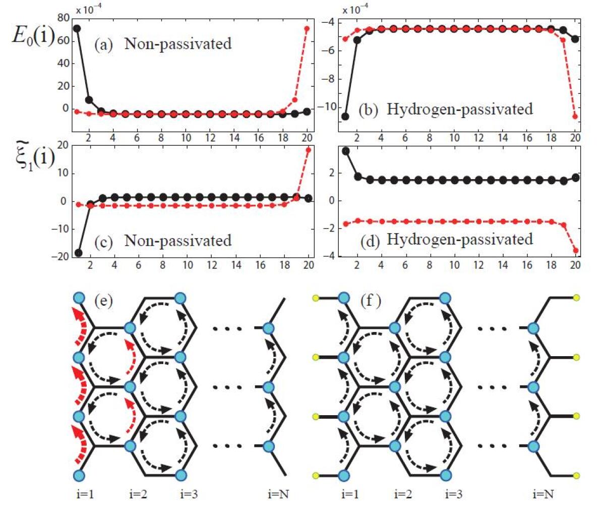
Figure 6: (Color online) The spatial dependence of the on-site energy $E_{0}(i)$ and the effective n.n.n hopping parameter $\tilde{\xi}_{1}(i)$ in eV for the non-passivated and hydrogen passivated ZGNR with width $N=20$ and $\tilde{\xi}_{1}(i)=\xi_{1}(i)/3\sqrt{3}$. $E_{0}(i)$ and $\tilde{\xi}_{1}(i)$ are plotted in (a) and (c) for the non-passivated ZGNR, while in (b) and (d) for the hydrogn passivated one. The dashed red and solid black curves are plotted for the A and B sublattices respectively. In (e) and (f), we depict schematically the signs and magnitudes of $\tilde{\xi}_{1}(i)$ for the counterclockwise hopping processes. The black(red) arrows mean that sign of $\tilde{\xi}_{1}(i)$ is $+(-)$ and their thickness represents the magnitude of $\tilde{\xi}_{1}(i)$.

References

- (1) C. L. Kane and E. J. Mele, Phys. Rev. Lett. 95, 146802 (2005)
- (2) C. L. Kane and E. J. Mele, Phys. Rev. Lett. 95, 226801 (2005)
- (3) N. A. Sinitsyn, J. E. Hill, Hongki Min, Jairo Sinova, and A. H. MacDonald, Phys. Rev. Lett. 97, 106804 (2006)
- (4) V. K. Dugaev, V. I. Litvinov, and J. Barnas, Phys. Rev. B 74, 224438 (2006)
- (5) Daniel Huertas-Hernando, F. Guinea, and Arne Brataas, Phys. Rev. B 74, 155426 (2006)
- (6) Hongki Min, J. E. Hill, N. A. Sinitsyn, B. R. Sahu, Leonard Kleinman, and A. H. MacDonald, Phys. Rev. B 74, 165310 (2006)
- (7) Yugui Yao, Fei Ye, Xiao-Liang Qi, Shou-Cheng Zhang, and Zhong Fang, Phys. Rev. B 75, 041401(R) (2007)
- (8) Xue-Feng Wang and Tapash Chakraborty, Phys. Rev. B 75, 033408 (2007)
- (9) J. C. Boettger and S. B. Trickey, Phys. Rev. B 75, 121402(R) (2007)
- (10) Andrew M. Essin and J. E. Moore, Phys. Rev. B 76, 165307 (2007)
- (11) Mahdi Zarea and Nancy Sandler, Phys. Rev. Lett. 99, 256804 (2007)
- (12) Seiichiro Onari, Yasuhito Ishikawa, Hiroshi Kontani, and Jun-ichiro Inoue, Phys. Rev. B 78, 121403(R) (2008)
- (13) Mahdi Zarea, Carlos Busser, and Nancy Sandler, Phys. Rev. Lett. 101, 196804 (2008)
- (14) P. K. Pyatkovskiy, J. Phys.: Condens. Matter 21, 025506 (2009)
- (15) A. H. Castro Neto and F. Guinea, Phys. Rev. Lett. 103, 026804 (2009)
- (16) Zhigang Wang, Ningning Hao, and Ping Zhang, Phys. Rev. B 80, 115420 (2009)
- (17) M. Gmitra, S. Konschuh, C. Ertler, C. Ambrosch-Draxl, and J. Fabian, Phys. Rev. B 80, 235431 (2009)
- (18) P. Ingenhoven, J. Z. Bernad, U. Zülicke and R. Egger, Phys. Rev. B 81, 035421 (2010)
- (19) Ralph van Gelderen and C. Morais Smith, Phys. Rev. B 81, 125435 (2010)
- (20) Manuel J. Schmidt and Daniel Loss, Phys. Rev. B 81, 165439 (2010)
- (21) Edward McCann and Mikito Koshino, Phys. Rev. B 81, 241409(R) (2010)
- (22) E. Prada, P. San-Jose, L. Brey and H. A. Fertig, e-print arXiv:cond-mat/10074910
- (23) D. Soriano and J. Fernández-Rossier, Phys. Rev. B 82, 161302(R) (2010)
- (24) D. Gosálbez-Martínez, J. J. Palacios and J. Fernández-Rossier, Phys. Rev. B 83, 115436 (2011)
- (25) R. Winkler and U. Zülicke, Phys. Rev. B 82, 245313 (2010)
- (26) Sergej Konschuh, Martin Gmitra, and Jaroslav Fabian, Phys. Rev. B 82, 245412 (2010)
- (27) Liang Fu and C. L. Kane, Phys. Rev. B 74, 195312 (2006)
- (28) J. E. Moore and L. Balents, Phys. Rev. B 75, 121306(R) (2007)
- (29) D. J. Thouless, M. Kohmoto, M. P. Nightingale, and M. den Nijs, Phys. Rev. Lett. 49, 405 (1982)
- (30) Yasuhiro Hatsugai, Phys. Rev. Lett. 71, 3697 (1993)
- (31) B. Andrei Bernevig, Taylor L. Hughes and Shou-Cheng Zhang, Science 314, 1757 (2006)
- (32) Markus Konig, Steffen Wiedmann, Christoph Brune, Andreas Roth, Hartmut Buhmann, Laurens W. Molenkamp, Xiao-Liang Qi and Shou-Cheng Zhang, Science 318, 766 (2007)
- (33) D. Hsieh1, D. Qian, L. Wray, Y. Xia, Y. S. Hor, R. J. Cava and M. Z. Hasan, Nature 452, 970 (2008)
- (34) Xiao-Liang Qi, Taylor L. Hughes and Shou-Cheng Zhang, Nature Physics 4, 273 (2008)
- (35) F. D. M. Haldane, Phys. Rev. Lett. 61, 2015 (1988)
- (36) G. Dresselhaus and M. S. Dresselhaus, Phys. Rev. 140, A401 (1965)
- (37) F. Guinea, e-print arXiv:cond-mat/10031618
- (38) Hai-Wen Liu, X. C. Xie and Qing-febg Sun, e-print arXiv:cond-mat/10040881
- (39) A. H. Castro Neto, F. Guinea, N. M. R. Peres and K. S. Novoselov and A. K. Geim, Rev. Mod. Phys. 81, 109 (2009)
- (40) R. Saito, G. Dresselhaus, and M. S. Dresselhaus, Physical Properties of Carbon Nanotubes (Imperial College Press, London, 1998)
- (41) L. Petersen, P. Hedegård, Surf. Sci. 459, 49 (2000)
- (42) Geunsik Lee and Kyeongjae Cho, Phys. Rev. B 79, 165440 (2009)
- (43) M.L. Elert, J.W. Mintmire, C.T. White, J. Phys. Colloques 44, C3-451 (1983)