Statistical Characterization of the Chandra Source Catalog

Abstract

The first release of the Chandra Source Catalog (CSC) contains $\sim$95,000 X-ray sources in a total area of  0.75% of the entire sky, using data from $\sim$3,900 separate ACIS observations of a multitude of different types of X-ray sources. In order to maximize the scientific benefit of such a large, heterogeneous data-set, careful characterization of the statistical properties of the catalog, i.e., completeness, sensitivity, false source rate, and accuracy of source properties, is required. Characterization efforts of other, large Chandra catalogs, such as the ChaMP Point Source Catalog (Kim et al. 2007) or the 2 Mega-second Deep Field Surveys (Alexander et al. 2003), while informative, cannot serve this purpose, since the CSC analysis procedures are significantly different and the range of allowable data is much less restrictive. We describe here the characterization process for the CSC. This process includes both a comparison of real CSC results with those of other, deeper Chandra catalogs of the same targets and extensive simulations of blank-sky and point source populations.

1. Introduction

The Chandra X-ray Observatory (CXO; Weisskopf et al., 2002) has observed an extremely diverse range of X-ray emitting astrophysical sources, ranging from spatially extended diffuse sources such as X-ray clusters to bright point-like sources such as Galactic black hole binaries. Even within the category of X-ray point sources, Chandra has observed the widest range of source X-ray fluxes of any previously flown X-ray satellite – spanning literally more than 10 orders of magnitude from the $\approx 10^{-18}\,{\rm ergs~{}cm^{-2}~{}s^{-1}}$ flux limits of the Chandra deep fields (Brandt et al., 2001; Giacconi et al., 2002; Alexander et al., 2003; Luo et al., 2008) to the $\approx 10^{-7}\,{\rm ergs~{}cm^{-2}~{}s^{-1}}$ of Sco X-1. These observations have occurred in a variety of instrumental arrangements, determined by whether or not either of the two gratings configurations (the High Energy Transmission Grating, HETG, Canizares et al. 2005, and the Low Energy Transmission Grating, LETG, Brinkman et al. 2000) was inserted into the optical path, and by which set of detectors (the Advanced CCD Imaging Spectrometer, ACIS-S and ACIS-I, CCDs, Garmire et al. 2003, or the High Resolution Camera, HRC-S and HRC-I, Murray et al. 2000) were placed in the focal plane. Although nearly all possible instrument/detector configurations have been used at some point over the mission lifetime, the majority of Chandra observations have been conducted with the ACIS CCDs inserted into the focal plane and without the use of any gratings. For this reason, the first release of the Chandra Source Catalog (CSC; Evans et al., 2010) consists solely of such observations.

The Chandra Source Catalog follows in the long tradition of using X-ray satellite observations to create surveys of detected sources, encompassing both those sources that were the targets of the original observing proposals and serendipitously discovered sources. Such past and present surveys include the Einstein survey (over 800 sources; Gioia et al., 1990), the ROSAT surveys of bright and faint sources ($\approx 20,000$ sources; Voges et al., 1999, 2000) and its counterpart WGACAT ($\approx 45,000$ sources; White, Giommi & Angelini, 1994), the ASCA Medium Sensitivity Survey ($\approx 1,200$ sources; Ueda et al., 2005), and the recent XMM-Newton survey (2XMM, with $\approx 247,000$ detections from 3,491 observations; Watson et al., 2009). What makes the CSC unique among these surveys is the unsurpassed (in the X-ray) spatial resolution of Chandra, which is $\approx 0.5^{\prime\prime}$ for on-axis sources. It is anticipated that over a 20 year lifetime, Chandra will conduct over 20,000 separate ACIS and HRC observations which will yield over 250,000 significantly detected X-ray sources. These sources already include a diverse set of objects spanning local sources within our own solar system to distant clusters of galaxies. The ultimate goal of the CSC is to represent the full diversity of Chandra observed sources, and to include both point-like and extended sources.

The initial release of the Chandra Source Catalog limits itself in several ways (Evans et al., 2010). As discussed above, it only considers ACIS observations without any inserted gratings. (A subset of no-gratings HRC observations was included as of release v1.1. Sources detected from the zeroth-order images of gratings observations eventually will be included.) Furthermore, source detections are derived from single observations, as opposed to merged observations from the same field. The Chandra Source Catalog does define “Master Sources” as distinct X-ray sources, which may be observed in more than one observation. However, Master Source properties such as position and flux are derived from appropriate combination of the corresponding properties from spatially coincident sources separately detected in individual observations. Other Master Source properties, such as inter-observation variability, are derived by collating and comparing properties from contributing sources detected in individual observations. Future releases of the CSC will include properties derived from data combined prior to source detection. The initial release of the CSC also limits sources to (physical and/or instrumental) source extents $<30^{{\prime}{\prime}}$. These restrictions of the initially released CSC can be compared to those found in a number of other released catalogs covering Chandra observations.

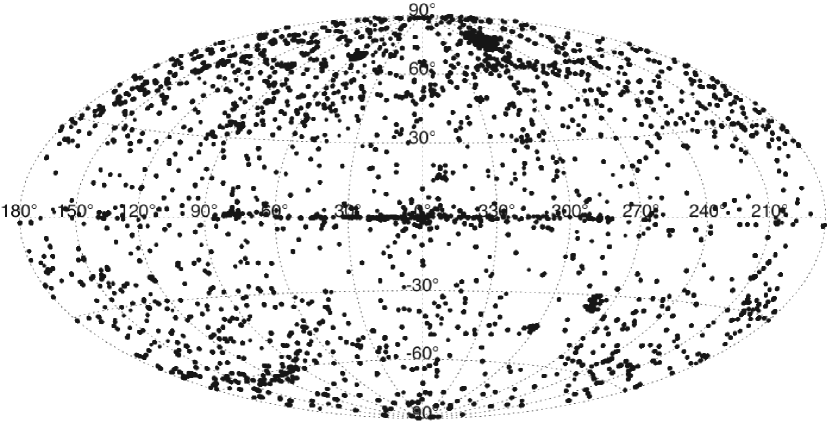
Figure 1.— Distribution of CSC sources on the sky, in galactic coordinates.

Numerous such Chandra catalogs already exist. Prominent among these are those that deal specifically with a well-defined set of fields of view. Examples of such targeted catalogs include the Chandra Deep Fields North (Brandt et al., 2001; Alexander et al., 2003, now containing over 500 sources) and South (Giacconi et al., 2002; Luo et al., 2008, with nearly 600 sources when including the flanking fields), and the Chandra Ultra-deep Orion Project (COUP; Getman et al., 2005, with over 1,600 sources). Although these catalogs currently consider source detections and properties from merged observations, they are far more restricted in terms of fields of view than the Chandra Source Catalog. More general catalogs include the Chandra Multi-wavelength Project (ChaMP Kim et al., 2004a, b, with nearly 1,000 sources); however, it too does not cover the full scope of fields of view as is covered by the CSC. Furthermore, these existing catalogs are all driven by the specific scientific goals of the projects that produced them. They do not share commonly defined source properties or analysis procedures.

The Chandra Source Catalog differs from these catalogs in several important respects. All data for all observations of a given Chandra detector are processed in a uniform manner with a uniformly defined set of source properties. The CSC also aims to be the most inclusive of any Chandra catalog. With few exceptions, all data from all active ACIS CCDs were searched for sources (see Evans et al., 2010, for a description of the criteria by which whole observations, or individual CCD detectors within an observation, were excluded). The intended audience for the CSC is not limited to X-ray astronomers nor to any particular sub-field of study within astronomy; it is intended as a general resource for all astronomers working at any wavelength.

Figure 2.— Distribution of livetimes for individual observations included in the CSC. The median livetime is $\sim 14$ ksec.

The Chandra Source Catalog is the product of a series of complex data processing pipelines. In order to take full advantage of the CSC products, users must understand the capabilities of both the Chandra observatory and the CSC analysis system. The CXO telescope and detectors have been documented extensively in numerous publications (Weisskopf et al., 2002; Garmire et al., 2003; Canizares et al., 2005; Murray et al., 2000; Brinkman et al., 2000). The CSC analysis system and first release products have been described by Evans et al. (2010). In this work, we describe in more detail the procedures used to characterize the capabilities of that analysis system, and the results of this characterization. The statistical characterization of the catalog source properties is accomplished primarily through the use of simulated datasets. These simulations include both empty fields (blank-sky) and simulated sources. For the most part, these simulated datasets are processed by the catalog pipelines in the exact same fashion as real datasets. We present here a summary of those results.

We begin with a summary of the overall properties of the source catalog. (See also Evans et al. 2010 for further descriptions.) We then describe the sky coverage of the first release catalog and discuss how limiting sensitivities within these fields of view are determined. In Section 4 we describe the algorithms used to create and assess our simulations. Results of these simulations are then presented in Section 5 for source detection, including the false source rate and the detection efficiency. Relative and absolute astrometry are discussed in Section 6. Photometry and source colors (hardness ratios) are discussed in Sections 7 and 8, respectively. Results of spectral fits for bright sources are described in Section 9. Estimates of source extents, and errors on these extents, are presented in Section 10. Section 11 deals with intra-observation variability within the catalog. We end with a summary of the current characterization efforts, and a discussion of plans for characterization efforts for future releases of the Chandra Source Catalog.

2. Overall Properties

The first release of the Chandra Source Catalog contains 135,914 individual source entries from 3,912 separate ACIS observations available in the Chandra Public Archive as of to Dec. 31, 2008. Because many Chandra targets were observed more than once, these individual source entries correspond to 94,676 unique “master sources”. These include both target and serendipitous sources. The distribution of sources on the sky, in galactic coordinates, is shown in Fig. 1. Individual observation exposure times ranged from $\sim 0.5-175$ ksec, with a median of $\sim 14$ ksec. The observation epochs range from Feb. 3, 2000 (Chandra MJD 51,577.5) to Dec. 31, 2008 (MJD 54,831.2), with a median of Jul. 1 2004 (MJD 53,187.3).

As can be seen in Fig. 2, the exposure time distribution exhibits strong peaks at multiples of 5 ksec., reflecting the inclination of Chandra Guest Observers to round required exposure times to these values when requesting observations. This may seem a trivial point, but it emphasizes an overwhelming dependence of the CSC on a heterogeneous mix of observations with different scientific objectives and requirements.

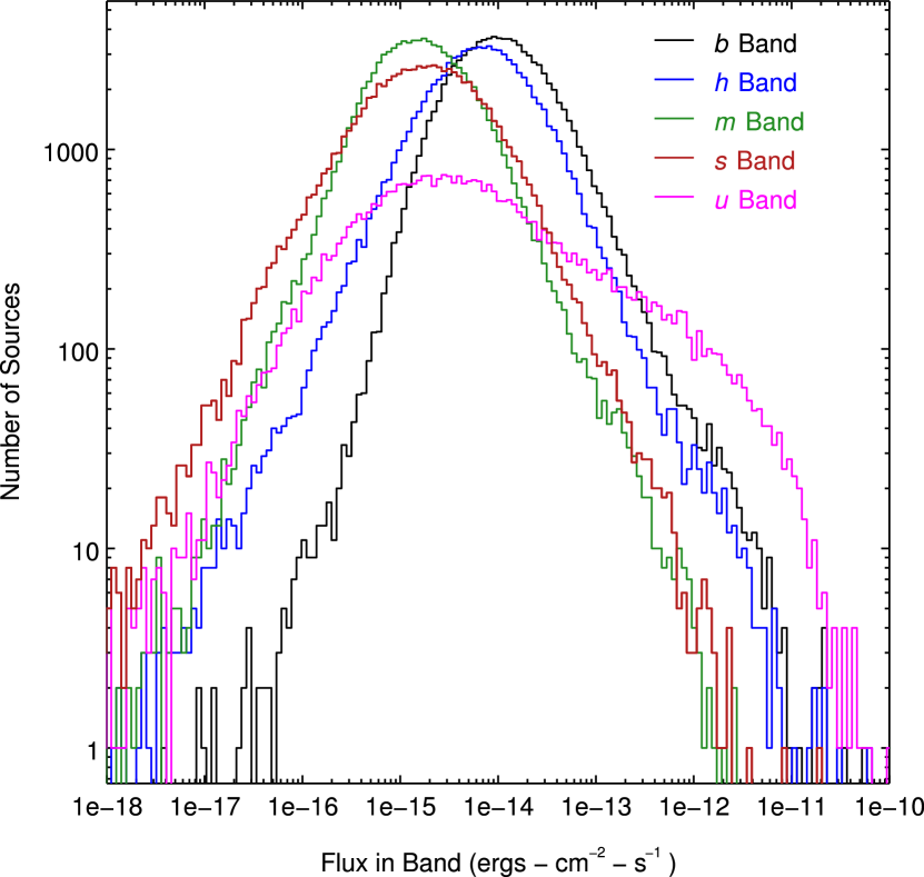
Figure 3.— Distribution of CSC fluxes in the broad (black), hard (blue), medium (green), soft (red), and ultrasoft (magenta) bands, obtained from the catalog master source table flux_aper columns.

CSC fluxes range from below $\sim 10^{-18}$ erg cm^-2 sec^-1 to $\sim 10^{-10}$ erg cm^-2 sec^-1. Most CSC sources have fluxes, as shown in Fig. 3, of $\sim 10^{-15}-10^{-13}$erg cm^-2 sec^-1 (b band, or 0.5-7.0 keV). We note that the u band number-flux distribution is much flatter that that observed in the other bands. Since photoelectric absorption is severe in the u band, it is tempting to attribute the flatter distribution to a population of relatively near-by sources. However, we caution against assigning any real astrophysical meaning to the distributions in Fig. 3 because they represent a hetergeneous mixture of sources of all types included in the CSC. The figure is intended merely to ilustrate the range of fluxes in the catalog. Minimum net source counts range from $\sim 10$ for on-axis sources to $\sim 15-30$ for sources with off-axis angle $\theta\sim 10^{\prime}$, depending on exposure.

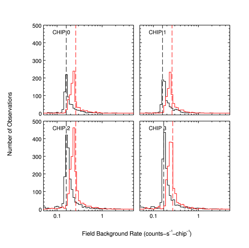
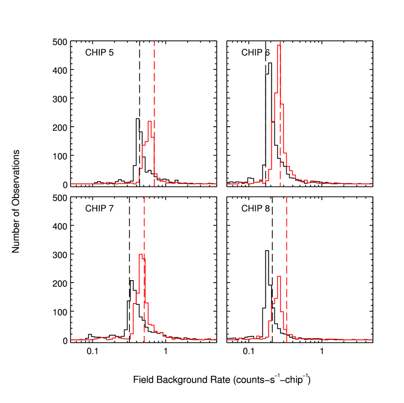
Figure 4.— Distribution of field background rates for commonly used ACIS imaging chips. Black (left) histograms refer to observations made prior to the median CSC epoch of July 1, 2004, and red (right) histograms to observations made after that date. Black and red vertical lines indicate nominal rates from v. 7 and v. 11 of the Chandra Proposers’ Observatory Guides, respectively.

CSC background rates are in general comparable to those reported in the Chandra Proposers’ Observatory Guide, and reflect the overall changes in background rate during the lifetime of the mission. This is illustrated in Fig. 4, in which we display histograms of background rates for chips 0–3 and 5–8, using observations taken before (black) and after (red) the median epoch. The background rates were determined by summing all b band events in each chip, subtracting b band net counts for CSC sources which fell on the chip, and dividing by the chip livetime. Nominal rates from v. 7 (black) and v. 11 (red) of the Observatory Guides are also shown.

Figure 5.— b Band limiting sensitivity map for OBSID 635. Each pixel value represents the minimum point source photon flux needed to yield a flux significance at the catalog inclusion limit, at that pixel location. Color bar units are photons-cm^-2-s^-1.

3. Limiting Sensitivity and Sky Coverage

A limiting sensitivity map is computed for each Observation Id (OBSID) that contributes to the Chandra Source Catalog, in each of the 5 science energy bands. The maps are derived from the CSC model background maps for the OBSID. Statistical noise appropriate to the observation is introduced by randomly sampling from Poisson distributions whose means are equal to the model background values in each map pixel. Each sensitivity map pixel represents the minimum point source photon flux needed to yield a flux significance greater than or equal to the catalog inclusion limit ($3\sigma$) at that location, when background is obtained from a region in the randomized background map appropriate to background apertures at that pixel location. The algorithm is described in detail in Evans et al. (2010). An example sensitivity map is shown in Fig. 5.

Because the limiting sensitivity maps are derived from model background maps, and not directly from the event data used to compute individual photon fluxes, it is important to demonstrate that they are consistent with the fluxes of sources included in the Chandra Source Catalog. We compare the photon fluxes of sources reported in individual OBSIDs in the CSC to the values of those OBSIDs’ sensitivity maps at the corresponding source locations. Photon fluxes for detected sources should all be greater than or equal to the corresponding limiting sensitivity values. The results for all bands are shown in Fig. 6. To simplify our procedure for matching source fluxes to limiting sensitivity, we have limited our sample of OBSIDs to those which included only a single Observation Interval (OBI). We find 120,230 sources with b band flux significances $\geq$ 3.0 in our sample, of which 464 ($\sim 0.4\%)$ have photon fluxes less than the expected limiting sensitivity value. The corresponding numbers for the u, s, m, and h bands are 112/4,552 ($\sim 2.5\%$), 538/50,052 ($\sim 1.1\%$), 595/57,480 ($\sim 1\%$), and 252/49,360 ($\sim 0.5\%$), respectively.

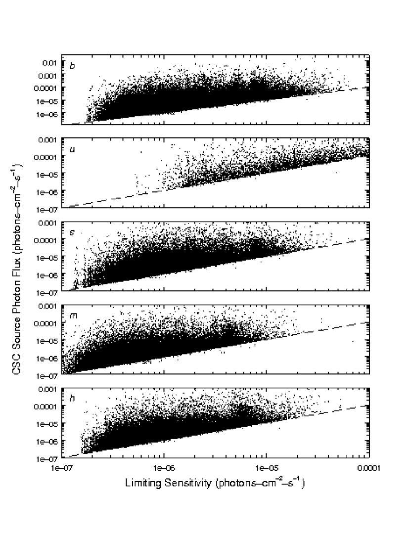
Figure 6.— Comparison of photon fluxes and limiting sensitivities in each band for sources with flux significances $\geq$3.0 in that band. Fluxes for reported sources should all fall on or above the dashed lines, for which flux and sensitivity are equal.

Although these percentages are small, it is worth examining the sources contributing to them in more detail. In Fig. 7, we show the 464 sources whose b band flux is less than the corresponding sensitivity. Of these, all but 21 are consistent with the threshold (dashed line) at which fluxes and sensitivities are equal, when flux errors are taken into account. Seventeen of these twenty-one are members of a set of CSC sources for which incorrect exposure times were used in calculating fluxes. The entire set includes 93 of the 464 sources in Fig.  7, shown in red, and $\sim 2,200$ sources in $\sim 160$ OBSIDs in the entire CSC. For these sources, exposure times for chips other than the source chip were used, leading to errors of $\sim 3\%$ or more in photon fluxes. Properties for these sources have been revised in Release 1.1 of the catalog. Two of the twenty-one are inconsistent with the sensitivity limit when 68% confidence bounds on flux are considered, but are consistent at the 90% level. For the remaining two sources, labeled by OBSID in Fig. 7, we find anomalous chip configurations. For OBSID 350, the target chip (chip 7) contained significant extended emission and was dropped from analysis; the source in question was located at the interface of chips 6 and 7. For OBSID 808, a subarray was used and the entire chip active area contained extended emission. In such cases, the background map algorithm fails and hence limiting sensitivity results are suspect. Similar results apply to the small percentages of failed sources in the other bands. We conclude that apart from these exceptional cases, the limiting sensitivities cited in the catalog are consistent with the actual distribution of measured source fluxes.

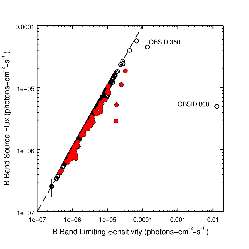
Figure 7.— b band photon fluxes and sensitivities for sources for which the photon flux is less than the corresponding limiting sensitivity. The dashed line represents the threshold at which fluxes and sensitivities are equal. One-sigma error bars are indicated for the faintest source, and are typical of the errors for all the sources. Red (halftone in paper edition) filled circles denote those sources whose fluxes are in error due to a bug in computing source exposure (see the discussion in Section 3). Labeled sources were observed in OBSIDs with anomalous chip configurations (see text).

Finally, we examine the behavior of limiting sensitivities with off-axis angle $\theta$. In Fig. 8 we reproduce the top panel (b band) of Fig. 6, but now displaying different ranges of $\theta$ separately. We find that for $\theta\leq 10^{\prime}$, the distribution of photon fluxes is consistent with the $flux=sensitivity$ threshold. However, for $\theta>10^{\prime}$, the flux distribution does not extend down to the threshold (Fig. 8, right panel). The differences amount to $\sim 10\%$, as indicated by the dashed red line at $flux=1.1~{}\times~{}sensitivity$, and may be interpreted as either an overestimate of fluxes or underestimate of sensitivities by this amount. Since there is some evidence from simulations for a slight overestimate of fluxes in this range of $\theta$, we consider the former possibility to be the most likely case here.

The sky coverage represents the total area in the CSC sensitive to point sources greater than a given flux, as a function of flux. We estimate sky coverage by assigning all non-zero limiting sensitivity map values to all-sky pixels, using the HEALPix projection (Górski et al., 2005), keeping only the most sensitive (i.e., lowest) value in each all-sky pixel. To reduce computational load and size of the projections (i.e., the number of HEALPix pixels), we rebinned the sensitivity maps to block 64 ($\sim 31.5^{{\prime}{\prime}}\times\sim 31.5^{{\prime}{\prime}}$), used $\sim 25.8^{{\prime}{\prime}}$ HEALPix pixels, and assigned rebinned sensitivity map pixels to the nearest HEALPix pixel, ignoring spillover. The resulting sky coverage function for the all bands is shown in Fig. 9. Total b band sky coverage is $\sim 320$ deg.².

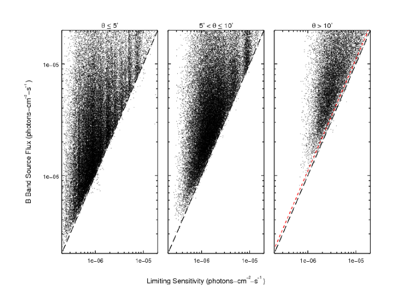
Figure 8.— Comparison of b band fluxes and sensitivities for sources in different ranges of off-axis angle. In each panel, the black (longdash) line represents the threshold at which fluxes and sensitivities are equal. For $\theta\geq 10^{\prime}$, the distribution of fluxes does not extend to this threshold, as indicated by the red (shortdash) line $flux=1.1\times sensitivity$. This indicates that either fluxes are over-estimated by $\sim 10\%$, or sensitivities are underestimated by a similar amount.

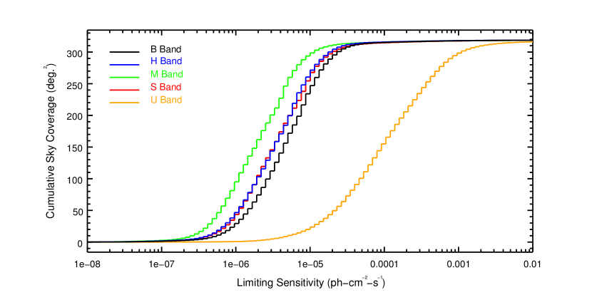
Figure 9.— CSC Sky Coverage for each science band. The value at each flux F represents the total CSC area sensitive to point sources with fluxes $\geq F$.

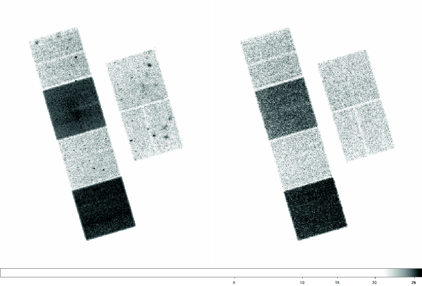
Figure 10.— Images of seed event list (left) and corresponding empty-field simulated event list (right) for 118 ksec ACIS-S observation 4613.

4. Simulation Algorithms

We use simulations of empty fields to estimate the number of false source detections in the catalog as a function of exposure, chip location, and detector configuration. We then inject simulated sources into these empty fields to investigate source properties such as position, flux, and extent.

In all cases except for variability studies, we start with actual observations that have been processed through the Chandra Source Catalog calibration pipeline. We selected four “seed” observations that span a wide range of exposures, for both ACIS-I and ACIS-S aimpoints. The set of seed observations is shown in Table 1. We then replace the actual event lists with simulated lists that share the same metadata, such as exposure, attitude, and detector configuration. These simulated event lists are then processed through the CSC source detection and properties pipelines.

We felt it necessary to adopt this “cuckoo’s egg” approach because of the complexity of the CSC software pipelines, in which multiple inputs to multiple programs could affect source detection or properties. We therefore treat the entire source detection and properties pipeline as a “black box” experimental apparatus, to be calibrated by studying its response to various artificial inputs. The exception to this approach is the characterization of source variability. In this case, it is simpler to simulate the variability analysis outside of the pipeline (see below).

Table 1Simulation Seed Observations

OBSID	Aimpoint	Exposure (ksec)	Chip Configuration
379	ACIS-I	9	0,1,2,3,6,7
1934	ACIS-I	29	0,1,2,3,6,7
4497	ACIS-I	68	0,1,2,3,6,7
927	ACIS-I	125	0,1,2,3,6,7
5337	ACIS-S	10	2,3,5,6,7,8
4404	ACIS-S	30	2,3,5,6,7,8
7078	ACIS-S	51	2,3,5,6,7,8
4613	ACIS-S	118	2,3,5,6,7,8

4.1. Empty Field Simulations

To simulate event lists containing background only, we start with the ACIS blank-sky data in the Chandra calibration data base. For each seed event list, we determine the appropriate blank-sky data sets for the active chips, using the CIAO tool acis_bkgrnd_lookup. The Chandra blank-sky datasets were adequate for all chips except chip 4 (S0), chip 8 (S4), and chip 9 (S5). For chip 8 we were unable to match the horizontal streaks in CSC data due to the different destreaking processing applied to the blank-sky datasets and the CSC event lists. For this chip, we constructed our own blank-sky dataset from CSC event lists of several long exposures that contained no bright sources in chip 8. Chip 4 and chip 9 have only one blank sky dataset at a focal plane temperature of -110 C. Given that they are very far off axis, and are not typically used in ACIS-S imaging observations, we have not included blank sky simulations for these chips. We expect that their characterization should be similar to other front-illuminated chips at large off-axis angles.

We estimate the expected number of background events for each chip from the chip nominal field background rate and observation on-time, and compute the ratio of this quantity to the number of events in the corresponding blank-sky dataset. For each chip column, we then determine the number of events by randomly sampling from a Poisson distribution whose mean is the number of events in that column in the blank-sky dataset, scaled by the event ratio. Row positions for these events are determined by randomly sampling from a normalized cumulative distribution derived from the row positions of events in the corresponding column of the blank-sky dataset.

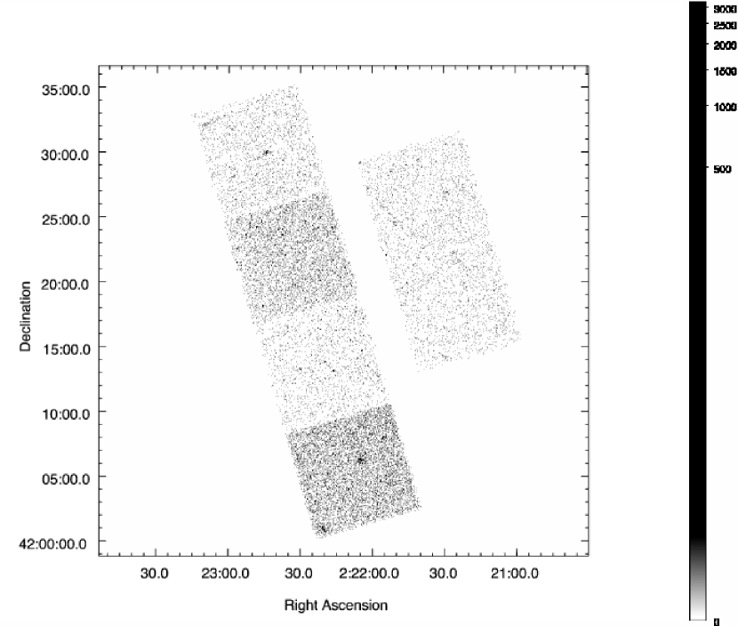
Figure 11.— An empty-field event list for ACIS-S observation 4613 with simulated sources inserted.

We simulate numbers of events and their positions in this fashion in order to preserve the column-to-column variations due to detector defects such as bad columns, and variations in quantum efficiency. The simpler technique of setting pixel values in simulated images to random samples from Poisson distributions whose means are the corresponding pixel values in the seed blank-sky images cannot be used because at the desired resolution the seed images contain zero-valued pixels. Since zero is an invalid mean for a Poisson distribution, appropriate random samples cannot be generated for such pixels, and simply setting the corresponding pixel values in the simulated images to zero would introduce unwanted statistical correlations in the set of simulated images for each seed obsid.

We approximated the nominal field background rates for each chip by values cited in the Chandra Proposers’ Observatory Guide, except for the longer ACIS-S observations (OBSIDs 7078 and 4613) which include chip 8. Here, since we were using an input blank-sky dataset derived from CSC event lists, we estimated the field background rates directly from source-free regions of the CSC event list for the longest exposure OBSID 4613. We found the rates to be $\sim$67% of the corresponding values from the Observatory Guide for chips 2, 3, 5, 6, and 7, and scaled the POG values by this amount. We attribute these differences to the more rigorous data screening in the CSC processing.

Finally, we distribute event times randomly within the good time intervals available for each chip, and re-compute the sky coordinates for the chip with the CIAO tool reproject_events, using the actual aspect solution from the seed observation. The final chip event lists are re-assembled into a single event list with the CIAO tool dmmerge. An example of a simulated event list for seed OBSID 4613 is shown in Fig. 10. Approximately 50 empty-field simulations were generated for each seed OBSID.

4.2. Point-Source Simulations

Simulated point sources were generated using MARX-4.3. A user-defined source model was input to MARX to generate X-ray photons incident from a spatially uniform random distribution of point sources, all having the same spectral shape of either a power-law (photon index $\Gamma=1.7$) or a blackbody ($kT=3.0$ keV), and with an absorbing column of $N_{\rm H}=3\times 10^{20}$ cm^-2.

More specifically, input source positions were generated by sampling from uniform random distributions of rotations about orthogonal axes aligned with directions of increasing Right Ascension and Declination, and offset from the observation aimpoint. These angular offsets were then converted to unit vectors in this coordinate system for input to MARX. They were also converted to Right Ascension and Declination using the coordinates of the aimpoint. The mean spatial density of randomly generated source positions was about 1.2 arcmin^-2. This source density was a compromise aimed at limiting source confusion and reducing the total number of simulations required to derive useful statistics on the performance of the software pipeline. A different random sequence was used to generate each simulated source population.

The source photon fluxes were drawn from a powerlaw distribution in which the number of sources, $N(f)df$ with photon flux between $f$ and $f+df$ is $N(f)df\propto(f/f_{0})^{-\alpha}df$ with $\alpha=1.5$. For a simulation based on an OBSID with exposure time $t$ in seconds, the minimum photon flux was $f_{0}=(0.003/A)(10^{5}/t)^{1/2}$ photons s^-1 cm^-2, where $A=2,269.55$ cm^-2 is the geometric area of the mirrors.

The effect of photon pileup (i.e., when two or more photons are recorded in a single CCD pixel in a single readout frame, and are either misinterpreted as a single event or discarded as a “bad” event) was included by post-processing each simulation with marxpileup. The effect of observation-specific bad pixels was included by post-processing each simulation with acis_process_events; events falling on bad pixels were flagged appropriately. Because the source and background components were created and processed separately and then combined only in the final step, we did not include the (negligible) effect of pileup due to coincidence between source and background photons.

To simulate an ACIS imaging observation based on a particular Chandra OBSID, two separate MARX simulations were usually required, one for the ACIS-I chips and one for the ACIS-S chips. Each simulation used the observation-specific aspect solution (asol file), detector position (SIM_Z), start time (TSTART), and exposure time (EXPOSURE).

The source events from the two MARX simulations were merged with the simulated background events, discarding all MARX-simulated source events on unused CCDs. After quantizing the background event arrival times to match the frame times of the relevant CCDs, the full set of event arrival times was sorted in ascending order. A table containing the coordinates of each simulated source and the associated flux in each spectral band was appended to the merged event file.

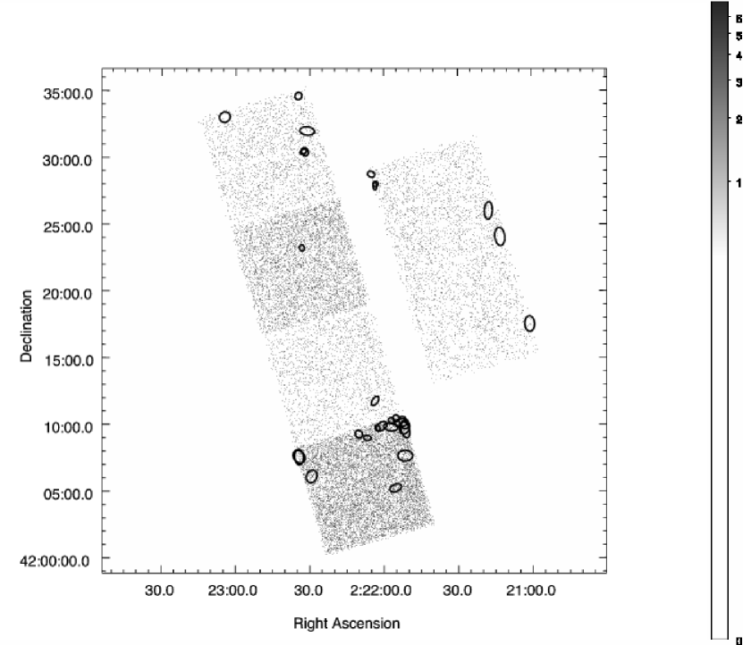
Figure 12.— An example simulated event list using the metadata for OBSID 4613. A total of 25 simulation runs were performed for this OBSID, yielding 30 source detections that passed CSC inclusion criteria. These detections are shown as black ellipses.

An example of an event list for seed OBSID 4613 with simulated sources inserted is shown in Fig. 11. Approximately 20 point-source simulations were generated for each seed OBSID, for each input spectrum, with $\sim 500-600$ sources per simulation. It should be noted that the distribution of fluxes for these simulated sources extends well below the anticipated CSC detection limit; the actual number of detected sources available for characterization analysis is approximately half the total number.

4.3. Variability Simulation Algorithms

To assess intra-observation variability, the Chandra Source Catalog employs three variability tests, described below, to assess whether event arrival times are consistent with the expectations for a steady source. Detected count rate variations for a steady source should be dictated solely by Poisson statistics and the time variable response of the spacecraft detectors. The latter is driven primarily by the effects of spacecraft dither. The pointing direction of the Chandra spacecraft is varied in a Lissajous pattern with typical periods of 1,000 and 707 seconds in perpendicular directions when observing with the ACIS detectors. Thus a source chip position can dither beyond the edges of the CCDs, or over detector locations with different responses or with different numbers of bad pixels, etc.

The algorithms for creating background simulations described in 4.1 reproduce very well the time averaged background with the proper counting statistics. The MARX simulations used to create the discrete source simulations (Section 4.2) essentially yield lightcurves that have the proper counting statistics for a steady source (i.e., white noise) dithering in a realistic time-dependent manner across the detector. The final simulations used to assess the CSC pipeline, however, are a combination of these time averaged and time-dependent components. Although these simulations are suitable for assessment of source detection, flux, and size algorithms, they are not suitable for detailed assessment of the source variability detection algorithms. This is especially true near chip edges where the effects of dither are expected to be the most significant. We plan to address these simulation shortcomings with future updates of the CSC characterization.

For this initial characterization we perform a series of lightcurve simulations and variability tests outside of both the MARX package and the CSC pipeline. These simulations thus lack detector details such as the CCD response and the spacecraft dither motion; however, they otherwise have been designed to mimic some properties of real Chandra lightcurves. The simulations have discrete time bins with 3.24104 sec resolution (the 41.04 ms ACIS readout deadtime is not included in the simulations), total lengths ranging from 1–150 ksec, and count rates ranging from 0.0006–0.03 cps (corresponding to 0.002–0.1 counts per readout frame). The goals of the simulations were to determine the rate of false positives for pure “white noise” simulations and to determine the sensitivity of the tests to real variability for “red noise” simulations.

The three intra-observation variability tests performed in the CSC pipeline are the Kolmogorov-Smirnov (K-S) test (essentially as described and implemented by Press et al. 2007), its variant the Kuiper test (Kuiper 1960; also based upon the implementation of Press et al. 2007), and the Gregory-Loredo variability test (Gregory & Loredo, 1992). Statistical properties and sensitivity of the first two of these tests are described by Stephens (1974). Essentially one is comparing the cumulative fraction of all lightcurve events that occur between the start of the observation and some given time, $t$, to the theoretically expected cumulative fraction also at time $t$. For a steady source, the latter is a curve that rises from 0 to 1 in direct proportion to the detector area-weighted “good time” that has elapsed. The K-S and Kuiper tests assess the significance of the maximum deviations of the measured cumulative fraction curve compared to the theoretical one. It is straightforward to incorporate time-dependent changes in detector efficiency into both of these tests.

Table 2CSC False Source Rates

OBSID	ACIS Configuration	Exposure (ksec)	#Sources (#Runs)	False Source Rate
379	ACIS-I	9	0 (50)	0.0
1934	ACIS-I	29	0 (50)	0.0
4497	ACIS-I	68	11 (50)	0.22
927	ACIS-I	125	64 (50)	1.28
5337	ACIS-S	10	1 (50)	0.02
4404	ACIS-S	30	5 (50)	0.12
7078	ACIS-S	51	5 (24)	0.21
4613	ACIS-S	118	30 (25)	1.2

The Gregory-Loredo test is a Bayesian algorithm that takes a given lightcurve and successively divides it into a greater number of uniformly spaced time bins. It then compares the Poisson likelihood that these uniformly binned lightcurves are a more probable description than the single bin lightcurve (Gregory & Loredo, 1992). The algorithm also returns a “best estimate” of the time-dependent lightcurve. Time-dependent detector variations can be incorporated into this test, but only in an approximate way. The algorithm implicity assumes that there is no correlation between the intrinsic variability time scales of the source and the variability time scales of the detector efficiency. Additionally, the Gregory-Loredo algorithm is testing a more specific hypothesis than the K-S and Kuiper tests. The latter tests are assessing the significance of any deviations from the expectations for a steady source. The Gregory-Loredo test is specifically examining the significance of uniformly binned lightcurves. These differences will be discussed further in Section 11.

In our simulations, all three of the above tests were implemented as S-lang scripts run via ISIS (Houck & Denicola, 2000). The scripts for the K-S and Kuiper tests were the same as those run in the CSC pipeline, whereas the script for the Gregory-Loredo test was an independent version from the C-code implementation used in the pipeline. The S-lang script, however, was extensively tested against the C-code and found to give nearly identical results in all cases.

Lightcurve simulations were also performed with S-lang scripts run under ISIS. Two types of simulations were performed: “white noise” and “red noise” simulations. For the latter, we followed the Power Density Spectrum (PDS) based approach outlined by Timmer & Koenig (1995). Essentially, one creates an instance of a lightcurve using the mean PDS profile, where the PDS is normalized such that its integral over Fourier frequency is the lightcurve mean square variability. For each Fourier frequency bin, one draws a Fourier amplitude that is distributed as $\chi^{2}$ with two degrees of freedom times the square root of the PDS amplitude. The Fourier phase in each bin is independently and uniformly distributed between 0–2$\pi$. The Fourier spectrum is then inverted to create the lightcurve, and the lightcurve mean is normalized to a desired level. (Vaughan & Uttley (2007) refer to simulations of this type as following the “Davies-Harte” method, after Davies & Harte (1987), and discuss how this method can be generalized to include even more complex statistical properties.) For the case of a red noise lightcurve, the mean PDS was $\propto f^{-1}$ between $1/T$ and $f_{Ny}\equiv(2\Delta t)^{-1}$, where $f$ is the Fourier frequency, $T$ is the total lightcurve length, $f_{Ny}$ is the Nyquist frequency defined by the bin size of the lightcurve, $\Delta t$. The root mean square (rms) variability was also defined by the integral between those two frequencies.

Once the lightcurve was created, any time bins that fell below zero were truncated at zero. (This was required only for a few bins in each lightcurve for rms variabilities $>10\%$.) The lightcurve amplitude in each time bin was then used to draw a Poisson variable for that time bin, which was used as the counts for the time bin. Note that the simulation process for the white noise lightcurves began at this point. Time bins with multiple counts were considered to be potentially subject to the effects of pileup, following the simple pileup model of Davis (2001). For each count in a single time bin in such cases, we assigned a 0.95 chance that it fell within the central “piled region”, and then drew a random variable (to be compared to the binomial distribution) to determine how many of the events were within this region. Once that number, $n$, was determined, a probability $\alpha^{n-1}$ was assigned to all the piled region events being read as a single event, with $1-\alpha^{n-1}$ being the probability that no counts would be registered for the piled region. This procedure then yielded the final lightcurves to which each of the above three variability tests was applied.

5. Source Detection

5.1. False Source Rate

To estimate false source rates, we conducted a series of blank-sky simulations at exposures of $\sim 10$, $\sim 30$, $\sim 60$, and $\sim 120$ ksec, for typical ACIS-I and ACIS-S chip configurations, as discussed in Section 4.1. Each simulated event list was then processed using the standard CSC source detection and properties software, and the resulting source detections that would have been included in the catalog were tabulated. The results are shown in Table 2, and an example simulated observation is shown in Fig. 12.

As can be seen in Table 2, the false source rate is appreciable only for exposures longer than $\sim$50 ksec. There is also some evidence for a clustering of false source detections near chip edges and between the back- and front-illuminated chips. To investigate these effects further, we considered the longest ACIS-I and ACIS-S simulation sets, and examined the false source rate separately near chip edges and interfaces. The results for OBSID 927 are shown in Fig. 13 and for OBSID 4613 in Fig. 14, and demonstrate that false source rates are enhanced in these regions.

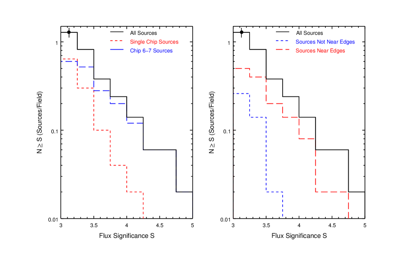
Figure 13.— False source rates as a function of flux significance for OBSID 927. The maximum flux significance of all science bands is used. Left: Single-chip sources are those whose source regions cover only a single chip, as indicated by the multi_chip_code. Chip 6-7 sources are those whose source regions dither across chips 6 and 7. Right: Sources near edges are those whose source regions dither off a chip edge during the observation.

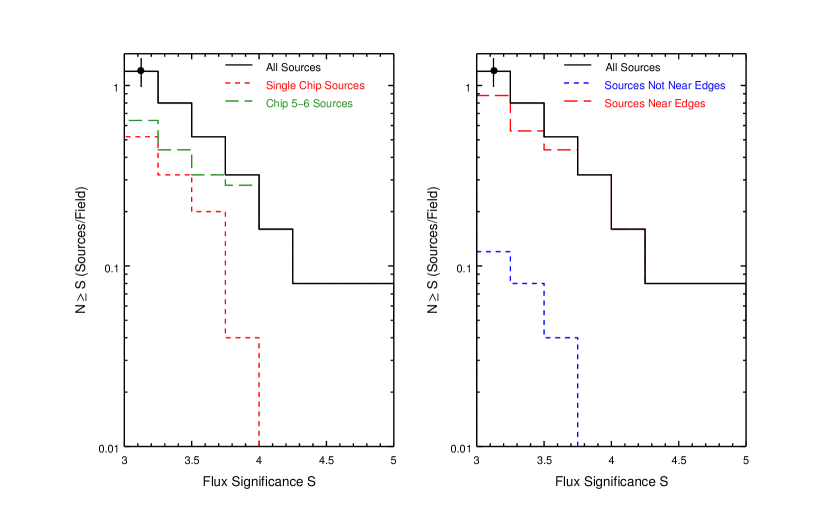
Figure 14.— False source rates as a function of flux significance for OBSID 4613. The definitions for different subsets are the same as in Fig. 13.

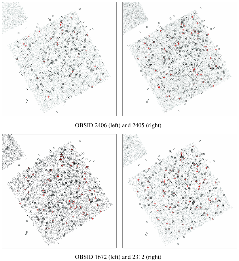
Figure 15.— CSC (crosses) and CDFS (circles) sources in four CDFS OBSIDs of $\sim 30$, $\sim 60$, $\sim 95$, and $\sim 124$ ksec. False sources, indicated by black arrows, are evident only for the longest exposure.

We can verify the conclusions of our simulation studies by examining CSC sources detected in individual observations that are themselves parts of longer-exposure observing programs. We use the Chandra Deep Field South (CDFS) Catalog of Alexander et al. (2003), which contains 326 sources in a total exposure of $\sim 940$ ksec, comprising 11 separate ACIS-I observations with similar aimpoints. Since source detection is performed on the deeper, combined CDFS images, we assume the CDFS catalog is complete at the level of individual component observations, and that therefore any CSC sources detected in individual CDFS observations that do not match sources in the CDFS catalog are likely to be false sources. We are implicitly ignoring the possibility of long term variability, where a real source is marginally detected in a single observation, but falls below the detection level for the combined observations.

In Fig. 15 we show CSC sources detected in individual CDFS OBSIDs 2406 (30 ksec), 2405 (60 ksec), 1672 (95 ksec) and 2312 (124 ksec), together with sources in the CDFS catalog. For OBSIDs 2406, 2405, and 1672, all CSC sources match CDFS sources, consistent with false source rates of $<1$ per field shown in Table 2. For OBSID 2312, three CSC sources do not match sources in the CDFS catalog. The mean rate from Table 2 is 1.28 for an ACIS-I observation of this length. If we assume a Poisson statistical model for the false source distribution, the probability of finding three or more false sources is $\sim 14$%. We conclude that the false source rates determined from real Chandra observations are consistent with those derived from our simulations.

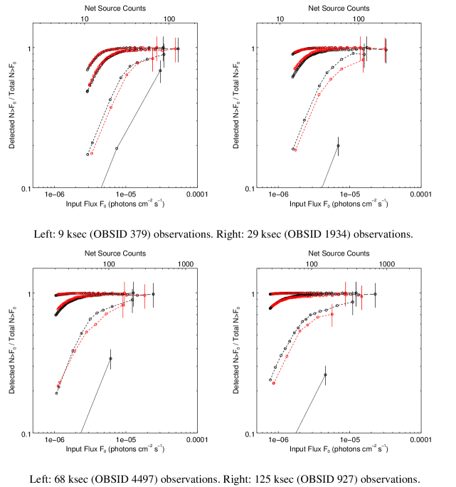
Figure 16.— Detection Efficiencies for simulated ACIS-I sources with powerlaw (black, left curve) spectra and blackbody (red, right curve) spectra, for sources with off-axis angle $\theta\leq 5^{\prime}$ (solid lines), $5^{\prime}<\theta\leq 10^{\prime}$ (long dash), $10^{\prime}<\theta\leq 15^{\prime}$ (short dash) and $15^{\prime}<\theta\leq 20^{\prime}$ (dot). Simple statistical error bars (i.e., $\sqrt{N}$) for the last bin are shown.

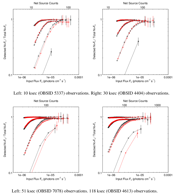
Figure 17.— Detection Efficiencies for simulated ACIS-S sources (see Fig. 16 for a description of the various components).

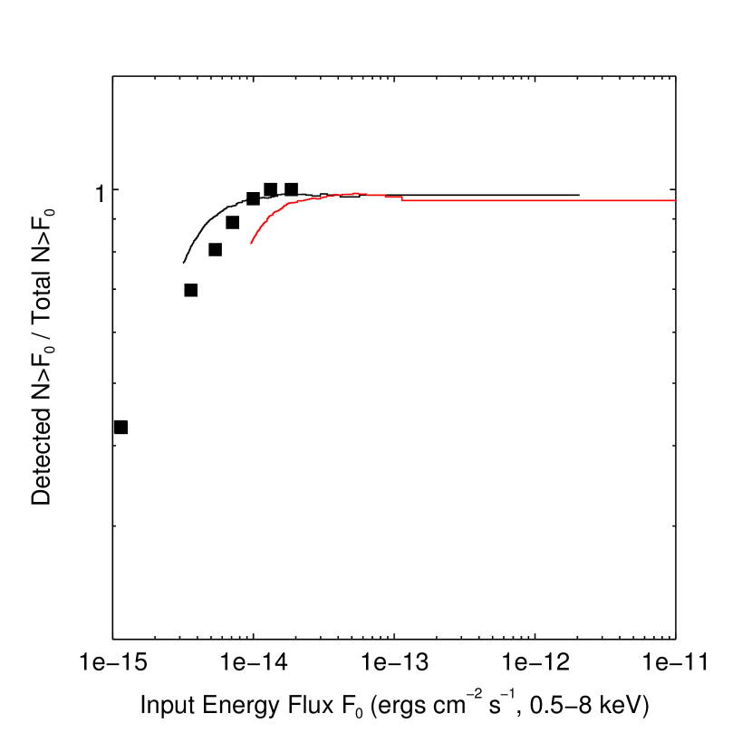
Figure 18.— Detection Efficiency for OBSID 2405, derived from sources detected in the CDFS catalog (Alexander et al., 2003). Efficiencies for powerlaw (black) and blackbody (red, or halftone in paper version of the article) sources in simulated ACIS-I observations of comparable exposure are included.

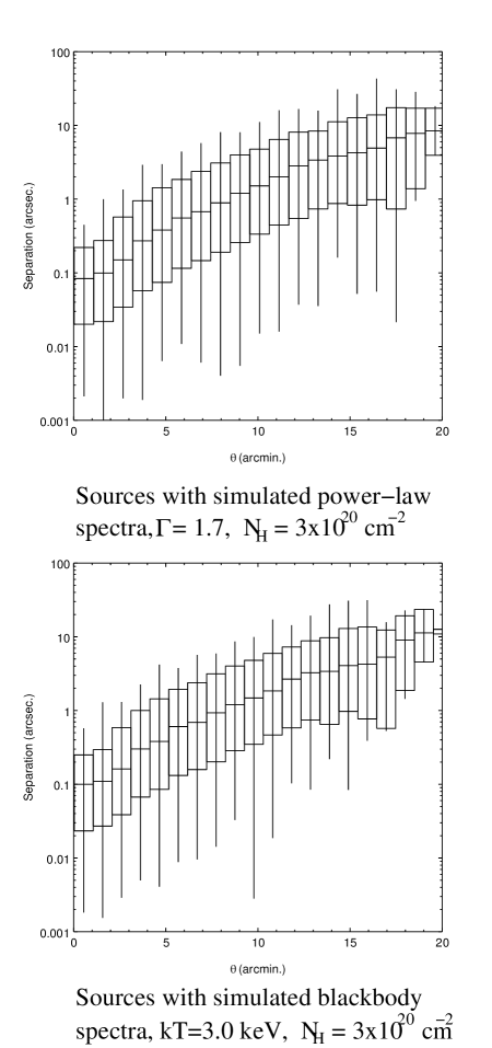
Figure 19.— Distribution of angular separations between input and measured source positions, as a function of source off-axis angle $\theta$. Median separations are indicated by horizontal lines. Boxes indicate the 95% (upper) and 5% (lower) percentiles of the distribution in each bin, and vertical lines indicate extreme values.

5.2. Detection Efficiency

We use the point-source simulations described in Section 4.2 to estimate detection efficiency as a function of exposure time for observations with ACIS-I and ACIS-S aimpoints. Sources with simulated powerlaw and blackbody spectra were analyzed separately; results were similar for both spectral models. Approximately 214,000 simulated sources were available for analysis, of which approximately half were detected by the CSC source detection pipeline and passed the quality assurance and flux significance criteria for inclusion in the catalog.

For each seed OBSID in Table 1 we constructed histograms of input b band photon fluxes for both detected and undetected sources, choosing bin boundaries such that there were 50 detected sources in each flux bin. We then constructed cumulative $N>S$ distributions from each histogram. The ratio of the distribution for detected sources to that for all sources represents the detection efficiency, i.e., the fraction of input sources brighter than a given incident flux that are actually detected. Results for the b band detections for the ACIS-I and ACIS-S simulation sets are shown in Figs. 16 and 17. Efficiencies are plotted against both input photon flux and net source counts. The latter are based on a linear regression between net counts and input flux for detected sources and are only intended to provide an approximate counts scale for the plots.

These curves are in general similar to those derived for the ChaMP Point Source Catalog (Kim et al., 2007), but are presented separately for standard ACIS-I and ACIS-S chip configurations, since the different chips sampled in each configuration may result in different efficiencies for certain ranges of off-axis angle $\theta$. For example, in the range $5^{\prime}<\theta\leq 10^{\prime}$, ACIS-I observations sample the relatively low-background, front-illuminated chips 0-3, while ACIS-S observations sample both the high-background, back-illuminated chip 7 and the badly-streaked chip 8. As indicated in Figs. 16 and 17, the detection efficiencies for the ACIS-S observations are systematically lower than those for the ACIS-I observations of comparable exposure in this range of off-axis angle.

Finally, we compare the detection efficiencies derived from our simulations to those measured from real Chandra observations, again using CSC sources detected in OBSID 2405 and the CDFS Catalog (Alexander et al., 2003). The CSC includes 72 sources with b band energy fluxes above $\sim 1.3\times 10^{-15}~{}{\rm ergs~{}cm^{-2}~{}s^{-1}}$ in ACIS chips 0-3 (those covered by CDFS) in OBSID 2405. All have counterparts in the CDFS catalog, which includes an additional 228 sources in the same field-of-view, with fluxes above $\sim 9\times 10^{-17}~{}{\rm ergs~{}cm^{-2}~{}s^{-1}}$ in the energy band from 0.5 to 8.0 keV. We use the CDFS fluxes in this energy band for both detected and undetected sources, to compute detection efficiency, using the procedure described previously. We chose bin boundaries to include 10 detected sources in each flux bin. To compare to the efficiencies from our simulations, we convert the input photon fluxes of our simulated sources to CDFS energy fluxes, using Sherpa (Freeman, Doe & Siemiginowska, 2001; Doe et al., 2007) and our powerlaw and blackbody spectral models. We find conversion factors of $3.03\times 10^{-9}~{}{\rm erg~{}photon^{-1}}$ for sources with powerlaw spectra and $8.56\times 10^{-9}~{}{\rm erg~{}photon^{-1}}$ for sources with blackbody spectra. We then computed detection efficiencies for simulated sources within $10^{\prime}$ of the aimpoint in ACIS-I OBSID 4497, which has an exposure time comparable to that of OBSID 2405. We do not divide the data into ranges of off-axis angle since CDFS sources typically contain contributions from multiple off-axis angles.

Our results are shown in Fig. 18 and indicate general agreement. We note that the CDFS sources exhibit a range of spectra, and their efficiency is bracketed by those derived from our two spectral models.

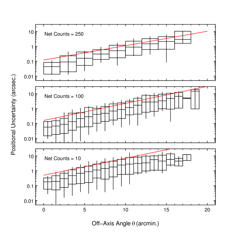
Figure 20.— Distribution of angular separations between input and measured source positions, as a function of source off-axis angle $\theta$, for three values of net counts. Red straight lines indicate the ChaMP 95% positional uncertainties, as reported by Kim et al. (2007).

Figure 21.— Fraction of simulated sources with position errors less than ChaMP 95% uncertainties, as a function of off-axis angle $\theta$, and net counts, for four exposure times used in the point-source simulations. Contours for fractions of 0.85, 0.9, and 0.95 are indicated.

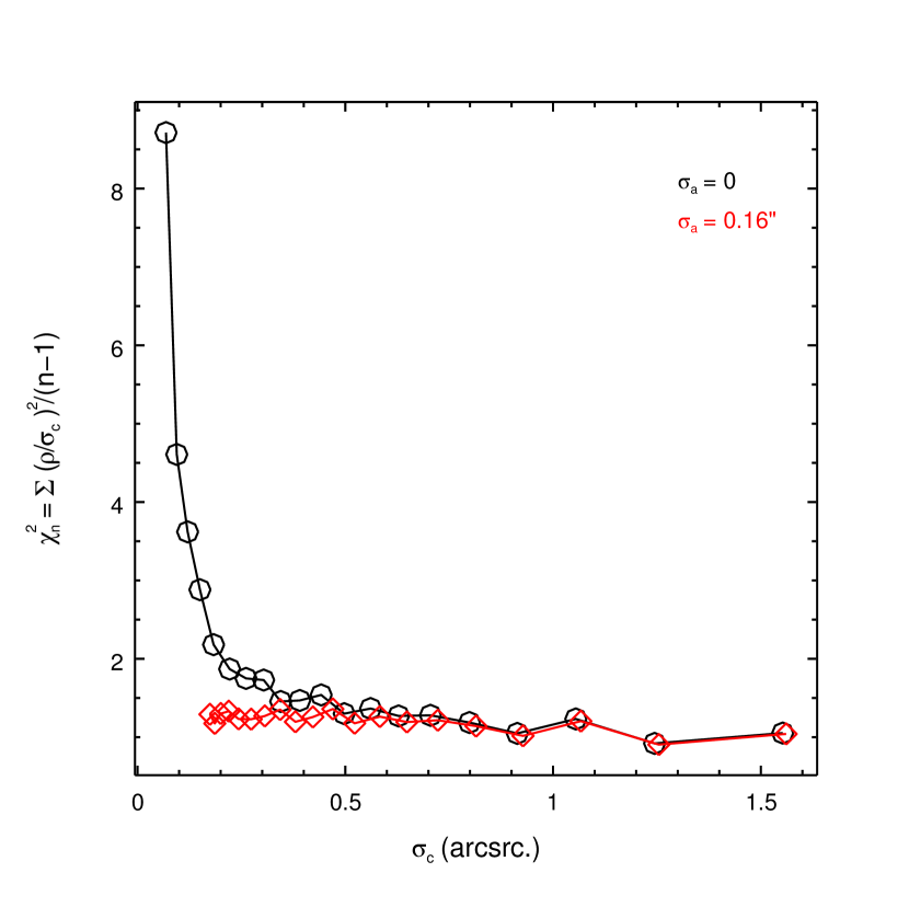
Figure 22.— Reduced $\chi^{2}$ vs. combined CSC-SDSS position error, for no assumed systematic astrometric error (black circles) and for a systematic error of $0.16^{{\prime}{\prime}}$ (red diamonds).

Figure 23.— Distribution of separations between input and source positions for all simulated sources (see Fig. 19 for an explanation of the meaning of various plot components). Also plotted as red filled circles are the average separations from the CSC-SDSS cross-match catalog. Dashed red horizontal lines are the medians in each bin with the astrometric systematic error added in quadrature.

Figure 24.— Average CSC-SDSS separations vs. average combined error for cross-match pairs in the bins used in Fig. 22. The combined errors include the $0.16^{{\prime}{\prime}}$ systematic astrometric error. The dashed line has a slope of 1.

6. Astrometry

Chandra Source Catalog source positions in individual observations are derived from centroids of events found in source apertures (Evans et al., 2010); their uncertainties are characterized by error circles whose sizes were determined from simulations generated by the ChaMP project (Kim et al., 2007) and verified in an earlier, limited set of CSC simulations. In the case of multiple detections of the same source, an error ellipse is derived from a combination of the error circles associated with the individual detections (Evans et al., 2010). To characterize the astrometric properties of the CSC, we first consider the accuracy with which we can locate sources in the frame of the observation, using simulated point sources. This can provide a good measure of the statistical uncertainty of the source position in the frame of the observation, but does not address any systematic errors in the absolute astrometry. To investigate these errors, we consider a subset of CSC sources with known counterparts of high astrometric quality, obtained from cross-matching CSC positions with positions from Data Release 7 of the Sloan Digital Sky Survey (Abazajian et al., 2009).

6.1. Statistical Uncertainties

To estimate the relative astrometric precision of the CSC, we use the point source simulations described in Section 4.2, and compare input and detected source positions. To be explicit, simulated sources are distributed in sky coordinates and rays are propagated onto chip coordinates using the MARX internal mirror and detector models. These simulations are passed through the CSC pipeline, where detected source positions are assigned to sky positions via knowledge of the spacecraft geometry. Thus the detected positions of the simulated sources are both a measure of the accuracy of the pipeline algorithms, as well as a measure of the fidelity of the MARX simulations. The correspondence between the MARX simulations and the true spacecraft geometry is explicitly discussed in the Appendix, and it is found to be excellent.

Approximately 90,000 simulated sources were identified by the CSC detection pipeline and meet the criteria for inclusion in the catalog. For these sources we have tabulated input source position and flux, detected source position and net counts from the CSC detection pipeline, and final source properties from the CSC properties pipeline. Distributions of angular separation between input and detected positions as a function of off-axis angle $\theta$ are shown in Fig. 19. Median separations range from $\sim 0.1^{{\prime}{\prime}}$ on-axis to $\sim 4^{{\prime}{\prime}}$ at $\sim 15^{\prime}$ off-axis. We find little difference in the results for the different input spectra, and so combine results from both in subsequent analysis.

We use these results to revisit the question of the suitability of the ChaMP error relations for the CSC. The ChaMP error relations are essentially functions of net counts and $\theta$ fit to particular percentiles of measured position error distributions at certain values of net counts and $\theta$. To examine how well they describe CSC position errors, we compare them to percentiles of CSC error distributions from our simulations, for appropriate values of net counts and $\theta$. In Fig. 20 we show three plots similar to those in Fig. 19, but now limited to sources with net counts within 10% of 10, 100, and 250 counts. The net counts used here are the quantities reported by wavdetect in the CSC source detection pipeline; these are the same quantities used to derive the ChaMP positional uncertainty relations and to calculate the error circles in the CSC pipeline. They differ slightly from, but are well-correlated with, the net counts determined from aperture photometry and reported in the catalog. The number of sources in each set are 2,341, 1,534, and 430, respectively. Also plotted are curves for the ChaMP 95% positional uncertainties from eq. 12 of Kim et al. (2007), for sources with 10, 100, and 250 net counts. For all three values of net counts, the ChaMP relations lie above the observed 95% percentiles (upper edges of boxes) for positional error distributions for $\theta\lesssim 3^{\prime}$. We conclude that the ChaMP uncertainties and hence the CSC uncertainties slightly overestimate the actual positional errors in this range. Similarly, for net counts=100 and 250, the ChaMP uncertainties appear to underestimate the true errors for $\theta\gtrsim 8^{\prime}$.

We investigate this result in more detail by constructing two-dimensional histograms in net counts and $\theta$, and computing the fraction of sources in each bin for which the separation between input and detected position is less than the ChaMP 95% positional uncertainty for that source. We divide our data into four subsets, corresponding to simulation exposures of $\sim 10$, $\sim 30$, $\sim 60$, and $\sim 120$ ksec (see Table 1). The number of sources in each subset are $\sim$13,000, 16,000, 29,000, and 32,000, respectively. If the ChaMP relations are always and everywhere a good measure of the CSC statistical position uncertainties, all histogram values should be $\sim$0.95. Images of the histograms are shown in Fig. 21, where we have lightly smoothed the histograms by a simple $3\times 3$ boxcar kernel, to aid in constructing contours. Only histogram bins containing more than 10 sources are shown. For exposures $\lesssim 30$ ksec, the ChaMP uncertainties are greater than the 95% percentiles of the actual position error distributions for net counts $\lesssim$40 and for most values of $\theta$ for which there are sufficient data. For higher exposures, the ChaMP uncertainties overestimate the actual 95% percentiles for low values of $\theta$, and underestimate the 95% percentiles at larger values, as suggested by Fig. 20. For all exposures, the ChaMP uncertainties approximate error distribution percentiles of $\gtrsim$80% for most of the range of net counts and $\theta$ for which we have sufficient data.

6.2. Absolute Astrometry

We have cross-matched the CSC with the SDSS DR-7 catalog (Abazajian et al., 2009), using the probabilistic cross-match algorithm of Budavári & Szalay (2008). We selected objects with a cross-match probability greater than $90\%$ and which were classified as stars in the SDSS catalog. The resulting cross-match catalog contained 6,310 CSC-SDSS pairs, corresponding to 9,476 sources detected in individual CSC observations, since many objects were observed several times by Chandra. We use the combined spatial error estimate of each object pair in this catalog as the independent variable and analyze the statistical distribution of the measured CSC-SDSS separations, $\rho$, to derive the value of any unknown CSC astrometric error. CSC provides a 95% error circle radius, while the SDSS provides independent 1-$\sigma$ errors in Right Ascension and declination (Pier et al., 2003). The combined error is derived by adding the geometric means of the major and minor axes for SDSS in quadrature with the CSC error and any unknown astrometric error, namely, $\sigma_{combined}=\sqrt{\sigma_{RA}\sigma_{Dec}+(0.4085\sigma_{{CSC}})^{2}+\sigma_{a}^{2}}$, where the numerical constant $0.4085$ is used to convert from a 95% to a 1-$\sigma$ error. The RA error bar is a true angular error bar in that a factor of $\cos(Dec)$ has been incorporated into it.

We sorted the cross-match pairs in increasing order of $\sigma_{combined}$ into bins containing $n=$100, 200, 300, and 400 sources for the first 4 bins, and 500 sources thereafter (the last bin contained 476 sources). We used smaller numbers in the first few bins since we assume that any unknown astrometric error, $\sigma_{a}$, is relatively small compared to the CSC uncertainties, especially off-axis, and that it therefore affects mainly those pairs with small combined errors. The statistical distribution of the separations will therefore change more rapidly for lower values of $\sigma_{combined}$. We characterized the statistical distribution of separations in each bin in terms of the reduced $\chi^{2}$ of the normalized separations $\rho_{N}=\rho/\sigma_{combined}$

$$\chi^{2}_{n}=\frac{\displaystyle\sum^{n}_{i=1}\rho_{N,i}^{2}}{n-1},$$ (1)

and examined the behavior of $\chi^{2}_{n}$ vs. the mean value of $\sigma_{combined}$ in the bins, for different assumed values of an unknown $\sigma_{a}$. As can be seen in Fig. 22, for $\sigma_{a}=0,\chi^{2}_{n}\sim 1$ for $\sigma_{combined}\gtrsim 0.25^{{\prime}{\prime}}$ but rises steeply below this value, validating our assumption that a systematic astrometric error dominates at small values of combined error. A value of $\sigma_{a}\sim 0.16^{{\prime}{\prime}}$ yields reasonable values of $\chi^{2}_{n}$ for all values of $\sigma_{combined}$, and we adopt this as our estimate for the CSC systematic astrometric error. Note, this value should be added in quadrature to all CSC 1-$\sigma$ positional uncertainties in Release 1.0.1 of the catalog. (This additional error is already incorporated into later catalog releases.)

We can use the CSC-SDSS cross-match catalog to verify the simulation results derived in Section 6.1. We show in Fig. 23 a plot similar to that in Fig. 19, but now combining results from both powerlaw and blackbody sources. We also plot the average CSC-SDSS separations in various bins in $\theta$. The CSC-SDSS separations agree well with the simulation results for $\theta\gtrsim 5^{\prime}$, but exceed the median simulation separations for smaller $\theta$. This result is to be expected since the simulation results do not include a systematic astrometric error, which dominates the CSC-SDSS results for the small separations prevalent at small $\theta$. When the systematic uncertainty is added (as indicated by the horizontal red lines), the results are in good agreement.

Finally, we use the CSC-SDSS results to investigate the suitability of the ChaMP errors, as in Section 6.1. In Fig. 24, we show the average CSC-SDSS separations as a function of $\sigma_{combined}$ for the data in the bins used to compute reduced $\chi^{2}$ above. For values of separation $\lesssim 0.7^{{\prime}{\prime}}$ (corresponding to $\theta\lesssim 7-8^{\prime}$ in Fig. 23) , the two agree well, but at larger values , $\sigma_{combined}$ becomes increasingly larger than the average separation, indicating that the ChaMP errors overestimate the true errors for $\theta\gtrsim 7-8^{\prime}$. This is roughly consistent with the results in Section 6.1, especially for exposures $\lesssim$30 ksec. We note the median exposure in CSC observations is $\sim$13 ksec.

Figure 25.— Comparison of input and measured b band fluxes for sources with powerlaw spectra. Bins in red contain fewer than 100 measurements; bins in blue contain 100-400 measurements; bins in black contain more than 400 measurements.

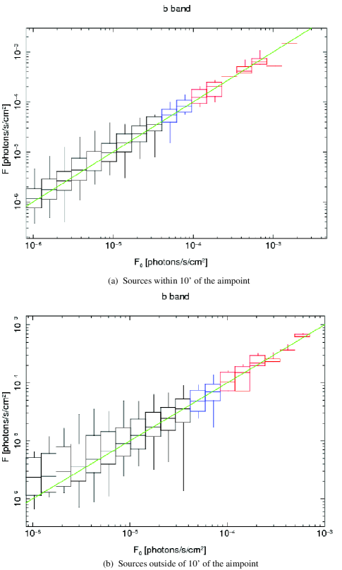
Figure 26.— Comparison of input and measured b band fluxes for sources with blackbody spectra. Bins in red contain fewer than 100 measurements; bins in blue contain 100-400 measurements; bins in black contain more than 400 measurements.

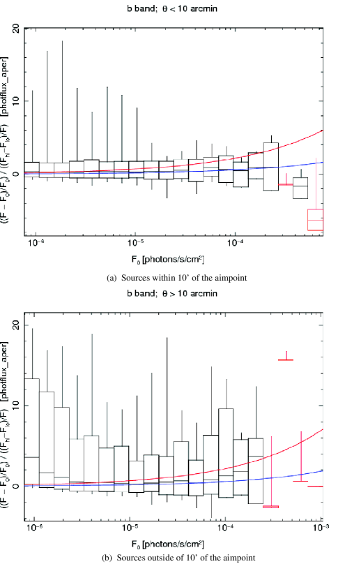
Figure 27.— Fractional difference between input and measured fluxes, normalized by measured fractional error, for sources with powerlaw spectra, in the b band. The smooth curves show the predicted systematic error for exposure times of 9 ksec (blue, lower curve) and 125 ksec (red, upper curve).

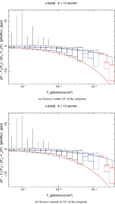
Figure 28.— Fractional difference between input and measured fluxes, normalized by measured fractional error, for sources with powerlaw spectra, in the s band. The smooth curves show the predicted systematic error for exposure times of 9 ksec (blue, upper curve) and 125 ksec (red, lower curve).

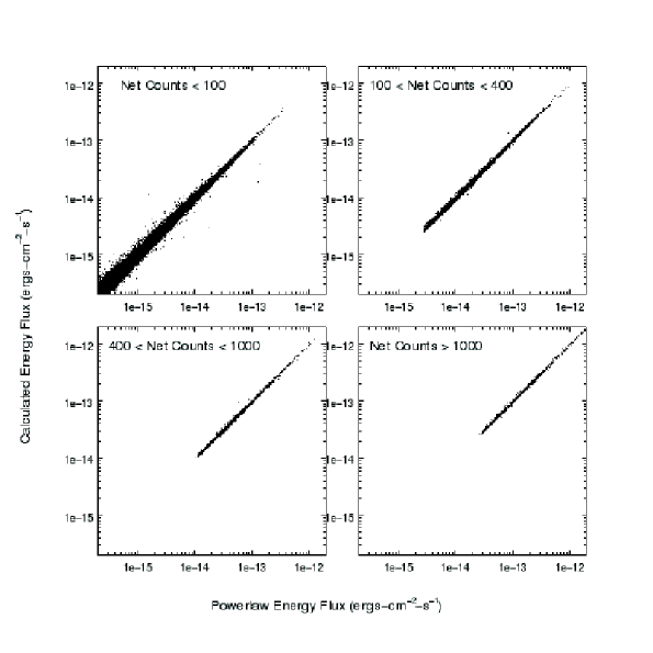
Figure 29.— Comparison of energy fluxes calculated from individual event energies and fluxes calculated assuming a powerlaw spectrum in the m band, for sources with 4 different ranges of m band net counts.

Figure 30.— Comparison of energy fluxes calculated from individual event energies and fluxes calculated assuming a powerlaw spectrum in the h band, for sources with 4 different ranges of h band net counts.

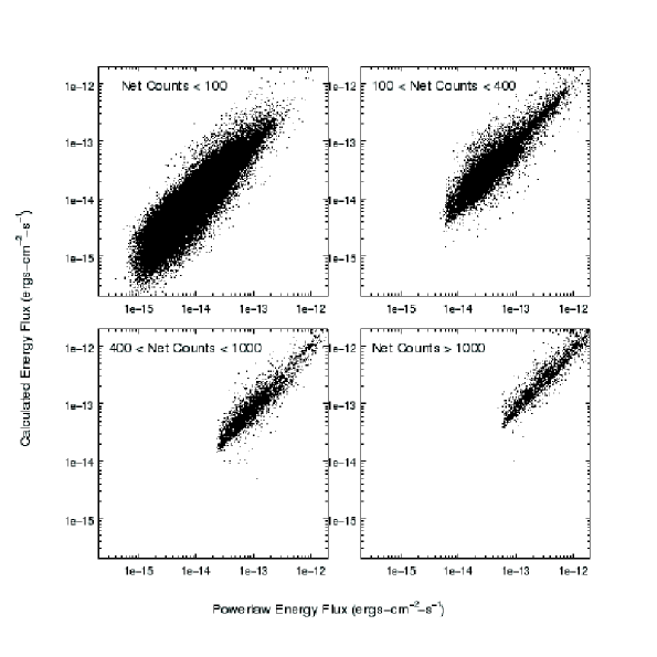
Figure 31.— Comparison of energy fluxes calculated from individual event energies and fluxes calculated assuming a powerlaw spectrum in the b band, for sources with 4 different ranges of b band net counts.

Figure 32.— Comparison of energy fluxes calculated from individual event energies and fluxes calculated from the sum of the powerlaw spectrum fluxes in the s, m, and h bands.

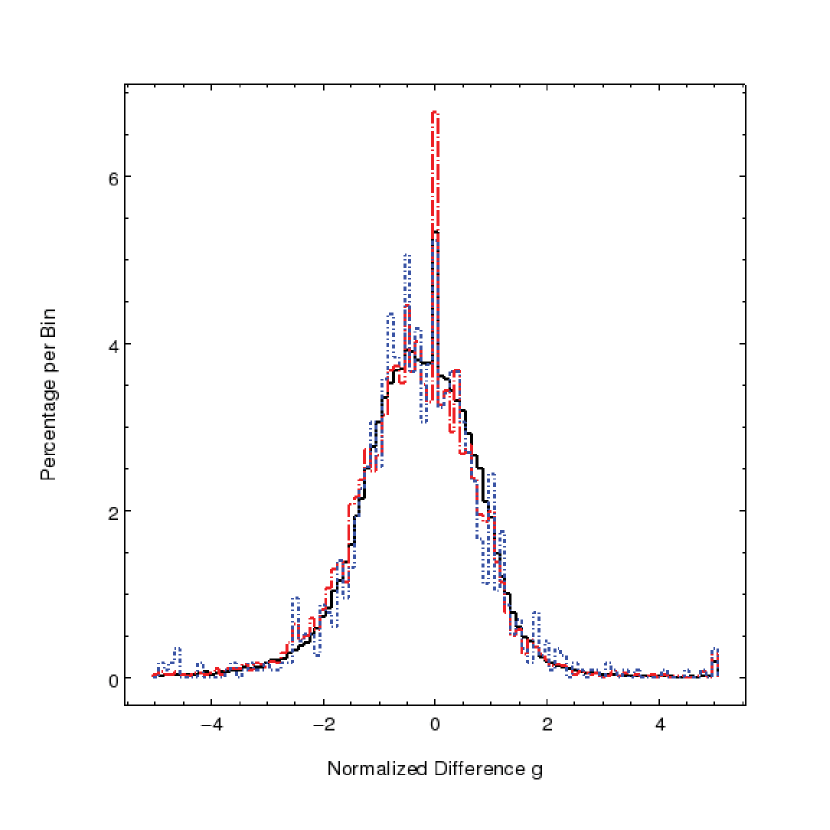
Figure 33.— Histogram of normalized differences between calculated and model h band energy fluxes for source with h band net counts less than 100 (black), between 100 and 400 (red, longdash) and between 400 and 1,000 (blue, shortdash). All histograms are normalized to sum to 100%.

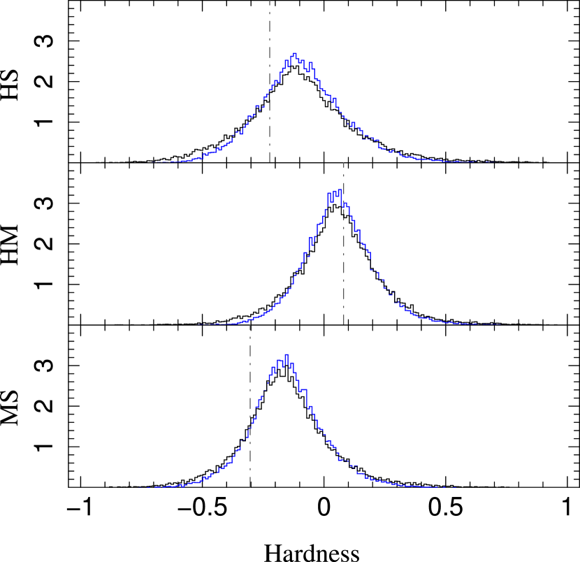
Figure 34.— Normalized histograms of catalog pipeline-derived hardnesses for simulated blackbody (top) and powerlaw (bottom) sources. HS represents the hard vs. soft bands, HM represents the hard vs. medium bands, and MS represents the medium vs. soft bands. Blue histograms are the hardnesses as calculated by the CSC implementation of the Park et al. (2006) algorithm. Black histograms are the hardnesses calculated from the catalog derived aperture photon fluxes. The vertical lines are the theoretical source colors for the ideal input models (i.e., using true model fluxes in a given band, not monochromatic estimated fluxes).

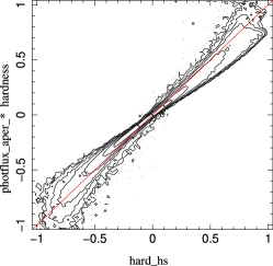
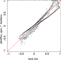
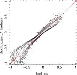
Figure 35.— Contours derived from two dimensional histograms comparing the CSC calculated hardnesses (horizontal axes) to the hardness directly calculated from the aperture fluxes (vertical axes). The left figure is for the hard vs. soft channel, the middle figure is for the hard vs. medium channel, and the right figure is for the medium vs. soft channel.

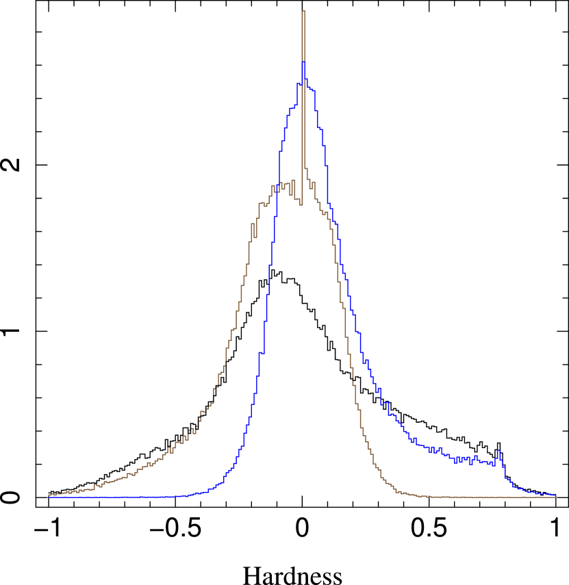
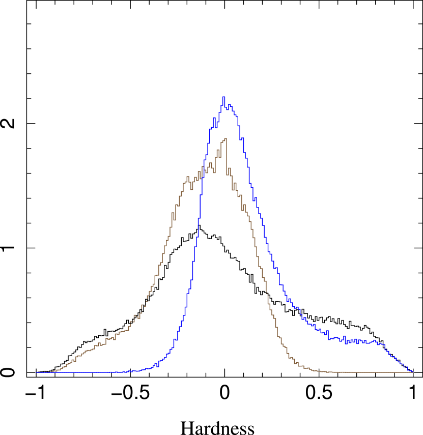
Figure 36.— Top: Normalized histograms of colors calculated directly from the aperture photon fluxes taken from the CSC v1.0.1. Bottom: Normalized histograms of the hard_* hardness values taken from the CSC v1.0.1 catalog. For both figures, the brown histogram is for the medium vs. soft bands, the blue histogram is for the hard vs. medium bands, and the black histogram is for the hard vs. soft bands.

7. Photometry

To assess the accuracy of Chandra Source Catalog source fluxes, we compare the input and measured fluxes of the simulated sources. We use fluxes derived from data in CSC source regions (photflux_aper). Fluxes derived from data in regions enclosing 90% of the local point response functions (photflux_aper90) are, in general, similar. Results for the powerlaw and blackbody simulation sets are shown in Figs. 25 and 26 for the b band and indicate good agreement for sources within $10^{\prime}$ of the aimpoint. For sources beyond $10^{\prime}$, there appears to be a systematic overestimate of a factor of $\sim 2$ for sources fainter than $\sim 3\times 10^{-6}$ ph-cm^-2-s^-1. We note, from Figs. 16 and 17, that detection efficiency for this range of off-axis angle is low and falling rapidly as flux decreases, and suggest that the flux overestimates are the result of an Eddington bias (Eddington, 1940), in which more sources with positive than negative statistical fluctuations in counts are detected near detection threshold. We have attempted to correct for the bias using the technique of Laird et al. (2009), but are able to account for only $\sim 10-20\%$ of the overestimate using their Equation 3. We note, however, that we use a different likelihood function to explicitly account for source contamination in background apertures (see Section 3.7 of Evans et al. (2010)). This may account for the differences, although we cannot exclude the possibility of other systematic errors. Additional work is in progress to understand this effect.

We also examined the fractional difference between input and measured fluxes $(F-F_{0})/F_{0}$, normalized by the fractional errors in measured fluxes, $(F_{hi}-F_{lo})/F$. Here, $F_{0}$ and $F$ are the simulated and measured fluxes, and $F_{lo}$ and $F_{hi}$ are the lower and upper confidence bounds for the measured flux. Representative plots of this quantity are shown in Figs. 27–28 and indicate the presence of additional systematic errors at high flux limits, even for sources within $10^{\prime}$ of the aimpoint. The effect is more prominent in the s band (Fig. 28).

Preliminary analysis indicates the effect is due to the assumption of a monochromatic exposure map in computing source fluxes. This assumption can lead to systematic errors because it ignores the energy dependence of the telescope response. The size of the systematic error depends on both the telescope response and the shape of the incident spectrum, $S(E)$. For example, in the limit of perfect background subtraction in spectral band $X$, the ratio of the estimated photon flux, $F$, to the true photon flux, $F_{0}$, in that band is

$$\phi_{X}\equiv\left.\frac{F}{F_{0}}\right|_{X}=\frac{(A(\overline{E})T)^{-1}\sum_{h\in X}C(h)}{\int_{X}S(E)\,dE},$$ (2)

where the number of counts in each narrow pulse-height bin is

$$C(h)\equiv T\int_{\Delta E_{h}}R(h,E)A(E)S(E)\,dE,$$ (3)

$R(h,E)$ is the redistribution matrix, $T$ is the exposure time, $A(E)$ is the effective area, and $A(\overline{E})$ is the effective area at energy $\overline{E}$ used to estimate the photon flux in the band of interest (which includes $\overline{E}$). In equation 2, the integral in the denominator spans the incident photon energies, $E\in X$, while the integral in the equation 3 spans all incident photon energies that contribute counts to the narrow pulse height bin, $E\in\Delta E_{h}$ .

To estimate the size of the systematic error defined by equation 2, we selected from CSC release 1.1 the response functions for 282 catalog sources with flux_significance_b$>5$ in the obsids listed in Table 1. These obsids were observed between May 2000 and July 2006 and represent a reasonable sample of the time-dependent ACIS detector contamination in the CSC. For each source in this arbitrary sample, we computed $\phi_{X}$ in each band for both the powerlaw and blackbody spectral models from §9, using the CSC-archived response functions. Within this sample, the systematic errors from the m and h bands have no significant time dependence because those bands are relatively unaffected by the increasing amount of detector contamination; for this sample, $\phi_{m}=0.94-1.04$ and $\phi_{h}=0.79-0.90$ for both powerlaw and blackbody spectra. The increasing detector contamination has a more noticeable effect on the s- and b-bands, introducing a weak time-dependence within the range $\phi_{s}=0.62-0.78$, $\phi_{b}=0.90-1.25$ for powerlaw sources and $\phi_{s}=0.90-1.0$, $\phi_{b}=1.12-1.28$ for blackbody sources. Flux measurements in the u-band are subject to large systematic errors for some spectral shapes; for the powerlaw spectrum, $\phi_{u}=0.80-2.4$, but for the blackbody spectrum, $\phi_{u}=1-25$.

The smooth curves in Figs. 27–28 illustrate the effect as a function of $F_{0}$. To generate these curves we used the ISIS fakeit command to simulate noise- and background-free powerlaw spectra for a range of $F_{0}$ and exposure times of 9 and 125 ksec, using canonical Chandra response functions. From these spectra we computed counts in the b and s bands, and their “statistical” ($\sqrt{n}$) errors and converted to “measured” flux and flux errors by dividing by exposure and $A(\overline{E})$ for the band. Although the resulting curves ignore contributions due to background subtraction and variations in Chandra response functions with time and detector, they do reproduce the general behavior of the observed values and add confidence to our explanation for the systematic errors at high fluxes.

As Evans et al. (2010) note, the method of calculating CSC energy fluxes by applying quantum efficiency and effective area corrections to individual event energies can be inaccurate for sources with few counts in energy bands where the Chandra effective area is small and changing rapidly. We have investigated this effect by comparing the energy fluxes calculated in this fashion with model fluxes calculated assuming our canonical power-law spectrum. Our results are shown in Figs. 29 and 30, respectively, and indicate good agreement for m band fluxes for all sources, but considerable scatter for sources with fewer than 100 counts in the h band. Results for the s and u bands are similar to those in the h band. For the b band, as indicated in Fig. 31, the fluxes show appreciable scatter even for sources with more than 100 net counts. We attribute this to the fact that some source spectra cannot be adequately approximated by a single power law in the b band. We note that when we compare calculated b band fluxes to the sum of powerlaw fluxes in the s, m, and h bands, the scatter is significantly reduced (see Fig. 32).

To quantify our results, we compute a normalized difference

$$g=(f-p)/\sigma$$ (4)

where $f$ is the energy flux calculated from individual event energies and effective areas, $p$ is the flux calculated using our canonical powerlaw spectrum, and $\sigma$ is defined as:

$$\sigma=\left\{\begin{array}[]{rl}f-f_{lo}&\mbox{ if $f\geq p$}\\ f_{hi}-f&\mbox{otherwise}\end{array}\right.$$ (5)

Here, $f_{lo}$ and $f_{hi}$ are the lower and upper bounds for the $1\sigma$ credible region for f. In Fig. 33, we show histograms of $g$ for h band fluxes in three separate ranges of net h band counts. In all three histograms, the percentage of sources with $|g|\leq 2$ is $\sim 90$%, compared with an expected $\sim 95$% for a Gaussian distribution.

Finally, we consider sources with zero counts or only an upper limit to the flux in one of the narrow bands. We examined events in the source regions of  7,000 discrepant sources with fewer than 20 counts, extracting the highest-flux photon in the broad band. For only $\sim 10$% of these sources did this photon contribute more than $\sim$50% of the total energy flux in the band; $\sim$3% percent had a single photon with $\sim$80% of the flux. This corresponds to only $\sim$0.2% of the entire catalog. The effect is reduced even further when background is accounted for. In several of the cases that we investigated in detail, the highest flux photon was actually compensated by a large subtracted background flux in that energy band. We conclude that $\sim 5$% of CSC sources may have underestimated energy fluxes or errors, but the number of cases in which a combination of a single photon and low background yield egregious flux estimates is negligible.

8. Hardness Ratios and Colors

The Chandra Source Catalog defines source hardness ratios that are meant to reflect the ratios of the aperture source photon fluxes (photflux_aper_*, in terms of the source properties columns). That is, in the high statistics limit, the source hardnesses are of the form

$$H_{xy}=\frac{F^{\gamma}_{x}-F^{\gamma}_{y}}{F^{\gamma}_{b}}~{}~{},$$ (6)

where $F^{\gamma}_{x}$ is the aperture photon flux in band $x$, $F^{\gamma}_{y}$ is the aperture photon flux in band $y$, and $F^{\gamma}_{b}$ is the aperture flux in the broad band. The concept behind the colors reflecting the values of the aperture photon fluxes is to partially normalize out variations induced by spatially and temporally dependent detector responses. Chief among these dependencies are the differing soft X-ray responses between the frontside and backside illuminated ACIS CCDs, as well as the time- and position-dependent ACIS contamination that has led to a decrease of the soft X-ray effective area over the lifetime of the mission. By using hardnesses related to aperture photon flux rather than solely counts or count rate, it is hoped that sources with the same intrinsic colors will yield similar estimated hardnesses regardless of observing epoch or detector position. Note that also as defined above, we expect hardnesses to be bounded between $-1$ and $1$.

In reality, the source hardnesses are calculated from the total counts (source plus background) in the aperture source region, the total counts in the background region, and scaling factors to convert from net source counts in the source region to aperture photon flux. The intrinsic hardness to be estimated is defined as

$$H^{i}_{xy}~{}\equiv~{}\frac{f_{x}x_{i}-f_{y}y_{i}}{f_{s}s_{i}+f_{m}m_{i}+f_{h}h_{i}}~{}~{},$$ (7)

where $x_{i}$, $y_{i}$, are the intrinsic source counts in bands $x$ and $y$, i.e., the soft, s, medium, m, or hard, h bands, and the broad band in this case is the sum of the individual bands. The factors $f_{*}$ are the conversion factors to transform from net source counts in the source region to source photon flux. These factors incorporate estimates of the detector effective area and exposure time in the given band, as well as the fraction of the point spread function within the source region.

The detected total counts will include a contribution from background counts that must be estimated. Furthermore, given the excellent sensitivity of Chandra to extremely faint sources, many faint CSC sources have zero net counts in one or two bands. The catalog estimates of hardnesses must account for these effects. To this end, the CSC employs an implementation of the Bayesian algorithm of Park et al. (2006). This algorithm, derived by considering the Poisson nature of the detected counts in both the source and background regions, is designed to be applicable even when no counts are detected in a given band. Furthermore, it is designed to yield a probability distribution for the hardness ratio that is properly bounded between $-1$ and $1$. Confidence limits are derived from this probability distribution, and thus never exceed an absolute value of 1. (This would not be guaranteed to be true if the hardnesses were determined, for example, by a Gaussian statistics approximation.)

To assess the success of the CSC implementation of the Park et al. (2006) algorithm, we have compared the calculated hardnesses for the simulated blackbody and powerlaw sources described in Section 5 to both the ideal expectations based upon the model input spectra, as well as to hardnesses directly calculated from the catalog aperture photon fluxes. These results are presented in Fig. 34. As can be seen from these figures, whereas the distribution of estimated hardnesses peak near the ideal model input hardnesses, there are biases in the hardness. Furthermore, these biases have the opposite sense for the blackbody vs. the powerlaw simulated spectra. The blackbody spectra are biased towards calculated colors that are too soft for hardnesses involving the hard channel. Conversely, the powerlaw spectra are biased towards calculated colors that are too hard for hardnesses involving the soft channel.

We have previously noted the biases in the estimated photon fluxes in Section 7, and they have also been described in Section 2.5.2 of Evans et al. (2010). These biases predominantly arise from the assumption of a monochromatic energy band when computing the conversion factor from counts to photon flux. The form of eq. (7), however, requires such a single conversion factor in each band, in contrast to a conversion factor per event as is used in the calculation of the aperture energy fluxes. In general we expect that the fidelity between the “true” hardness and the estimated hardness will be spectrum and possibly detector-dependent.

The simulations show, however, that although the colors are biased, there is a very good agreement between hardness estimates whether they are taken from the catalog pipeline or whether they are calculated directly from the aperture photon fluxes. When looking at the results for the CSC as a whole, we find for the actual sources in the v1.0.1 catalog that this overall agreement between hardnesses derived from these two methods holds. In Fig. 35 we plot contours of 2-D histograms comparing the CSC results for these two estimates. The contours are tightly gathered around a unity-correspondence. This opens up the possibility for a catalog user to calculate the expected bias in the hardnesses from a hypothesized spectrum in a few test cases, and then using these calculated biases to inform an acceptable set of hardness filtering criteria.

Figure 37.— Comparison of input and fitted b band energy fluxes for sources with simulated power-law spectra.

Figure 38.— Comparison of input and fitted b band energy fluxes for sources with simulated blackbody spectra.

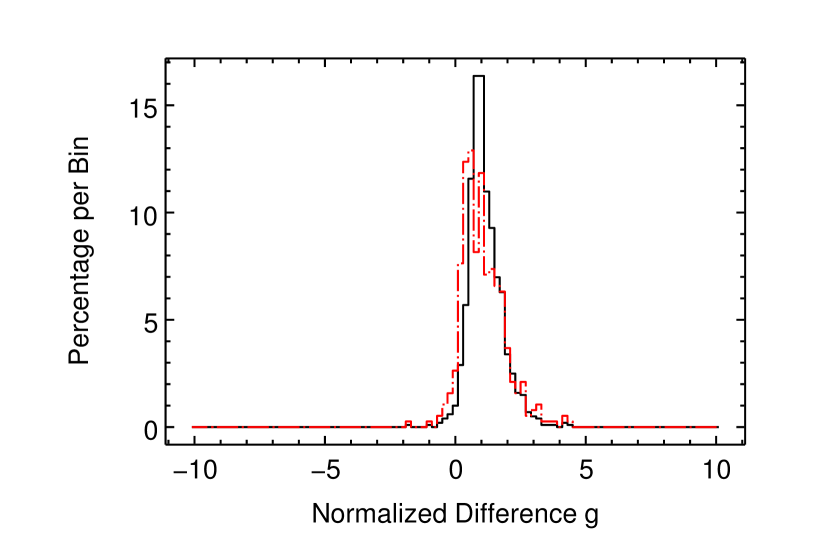
Figure 39.— Distribution of normalized differences between fitted and simulated spectral parameters for sources with more than 150 (black) and 500 (red, dashed) net b band counts: (top) power-law slope for 3,455 sources (black) and 802 sources (red, dashed); (bottom) $N_{H}$ for 1,002 sources (black) and 380 sources (red, dashed).

In Fig. 36 we show further results for real catalog sources, both when defining the colors via the aperture photon fluxes and as calculated via the application of the Park et al. (2006) algorithm. The catalog hardness histograms have peaks comparable to those of the powerlaw simulations, albeit with histogram tails that extend to both harder and softer colors. For hardnesses calculated directly from aperture photon fluxes, both the medium vs. soft histogram and the hard vs. medium histogram have local peaks at a hardness ratio of 0. These peaks are due to sources that were detected in only the hard band, or only in the soft band, respectively. As the Bayesian algorithm of Park et al. (2006) is specifically designed to properly handle cases with zero counts in a given band, these local peaks are smoothed out when applying this algorithm, as can be seen in Fig. 36.

9. Spectral Fits

For sources with more than 150 net counts in the b band, the Chandra Source Catalog attempts to fit the observed counts spectrum with both absorbed power-law and absorbed blackbody spectral models. We use the simulated spectra provided as part of our point-source simulations to characterize the results of CSC model spectral fits. We compare integrated b band model fluxes with input b band fluxes, using a subset of simulated sources for which aperture photometry yields more than 150 b band counts (src_cnts_aper_b), and for which successful spectral model fits were obtained . A total of 3,455 sources were used for power-law fits, and 2,897 sources for blackbody fits. Since the CSC reports integrated model fluxes as energy fluxes, we convert input simulated photon fluxes to energy fluxes using the known spectral parameters described in Section 4.2. We used conversion factors of $2.81\times 10^{-9}$ and $6.64\times 10^{-9}$ ergs  photon^-1 for power-law and blackbody spectra, respectively. Our results are shown in Figs. 37 and 38, and are in general similar to the results shown in Figs. 25 and 26, albeit with many fewer sources. In particular, the systematic flux overestimate for faint sources ($<\sim 1-2\times 10^{-14}$erg cm^-2 s^-1) at large off-axis angle is evident in the spectral model fits as well.

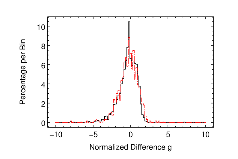
Figure 40.— Distribution of normalized differences between fitted values and simulated values for blackbody temperature $kT$. Black histograms refer to the entire sample of 2,897 sources. Red dashed histograms refer to the restricted sample of 669 sources with more than 500 net b source counts.

We compare fitted spectral parameters $\Gamma$, $kT$, and $N_{H}$, to input spectral parameters for the corresponding model simulations, using normalized differences like those defined in Section 7; we define $f=\Gamma_{fit}$ and $p=1.7$ for $\Gamma=1.7$ power-law spectra, $f=kT_{fit}$ and $p=3.0$ for $kT=3.0$ blackbody spectra, and $f=N_{H,fit}$ and $p=3.0\times 10^{20}$ cm^-2 for $N_{H}$ for both models. Our results are shown in Figs. 39 and 40. For power-law fits, we find a median $\Gamma$ of 1.724 for the 3,455 sources in our sample, with $\sim 96$% with normalized difference $|g|<2$. If we restrict the sample to sources with more than 500 net counts, we find a median $\Gamma$ of 1.718 for the 802 sources in the sample, with $\sim 93$% with $|g|<2$. For blackbody fits, we find a median $kT=2.90$ keV for 2,897 sources with more than 150 net counts, and a median $kT=2.96$ keV for 669 sources with more than 500 net counts. In both cases, $\sim 92$% had $|g|<2$. We note that for both power-law and blackbody models, the fitted spectra are slightly softer than the input spectra. This result is expected, since no energy-dependent aperture corrections are performed in spectral model fits. For the power-law fits, the median values of $\Gamma$ are consistent with the softening of $0.03-0.05$ in spectral index estimated in Section 3.9 of Evans et al. (2010).

For sources with simulated power-law spectra, fits converged to valid values of both $N_{H}$ and its lower confidence bound for only 1,002 sources in the full sample and for only 380 sources in the higher net count sample. For the remainder of the sources, the fitting procedure encountered the lower bound of the search region for $N_{H}$ ($1.0\times 10^{15}$ cm^-2) before encountering either the best-fit value or the lower confidence bound. In many cases, neither were included in the parameter search region. We excluded these sources from analysis of the $N_{H}$ distributions. The resulting distributions were skewed for both net count samples, as shown in panel (b) of Fig. 39. For the full sample, the median $N_{H}$ = $1.2\times 10^{21}$ cm^-2 with $\sim 92$% having $|g|<2$. For the higher net count sample, the median $N_{H}=6.7\times 10^{20}$ cm^-2 with $\sim 90$% having $|g|<2$. We note that most ($\sim 95\%$) sources in the full sample had fewer than 1000 net counts and conclude that $N_{H}$ is poorly determined in the CSC fits in this count range. We do not cite a result for $N_{H}$ for sources with simulated black-body spectra since most fits were unable to converge to valid best-fit values or confidence bounds in the range of parameter space used in the fitting routines. We attribute the additional insensitivity of the fitting statistic to $N_{H}$ to the relatively high temperature of 3 keV used to simulate the blackbody spectra.

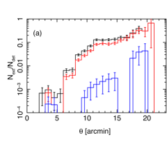
Figure 41.— Fraction of simulated (a) powerlaw and (b) blackbody point sources erroneously marked as extended in the b band as a function of off-axis angle, $\theta$, The black (top) histogram includes sources with (extent_code&0x10) != 0. The red (middle) histogram includes sources with (extent_code&0x10) != 0, pileup_warning$<0.01$, and (conf_code&0x3) = 0. The blue (bottom) histogram includes sources with (extent_code&0x10) != 0, pileup_warning$<0.01$, and (conf_code&0xf) = 0.

10. Source Extent

The raw extent of Chandra Source Catalog sources is parameterized by elliptical Gaussian sigma values (mjr_axis_raw_b, mnr_axis_raw_b). For each CSC source, a corresponding raw PSF elliptical Gaussian (psf_mjr_axis_raw_b, psf_mnr_axis_raw_b) is derived by processing an SAOSAC simulation using the same software. For robust comparisons of raw source size (RSS), it is convenient to define the RSS as $a\equiv\left(\sigma_{1}^{2}+\sigma_{2}^{2}\right)^{1/2}/\sqrt{2}$, where $\sigma_{i}$ are the elliptical Gaussian semi-axes. extent_code bits are set when the raw source size exceeds the PSF size by a statistically significant amount within the corresponding spectral band.

The method used to derive the elliptical Gaussian size parameters works well for isolated sources embedded in relatively smooth background emission, but it performs less reliably when the density of sources is high enough that source regions overlap. The ellipse derived for a confused point source may not give an accurate measure of the source size. For each catalog source, conf_code indicates the nature of the overlap with nearby sources. For example, (conf_code&0x3) = 0, indicates that the source detection region overlaps no other source detection region. (conf_code&0xf) = 0, indicates that the source detection region overlaps no other region and the background region overlaps no other source detection region.

Complicated image morphologies that arise from photon pileup in bright sources may also confuse automated source extent measurements. The associated pileup_warning value may be used to gauge the importance of photon pileup for a given source.

We define the false extent fraction, $f_{\mathrm{fx}}$, as the fraction of detected point sources that are erroneously identified as extended because of source confusion, or photon pileup, or any other reason such as a flaw in the method used. We used the MARX point source simulations described in §4.2 to estimate $f_{\mathrm{fx}}$ as a function of off-axis angle. Because the MARX-simulated sources are known to be point sources, any non-zero extent_code bit is, by definition, erroneous. Fig. 41 shows the b band false extent fraction as a function of off-axis angle for powerlaw and blackbody sources. The black curve shows the false extent fraction based solely on the extent_code determined from the measured raw sizes of source and PSF and the associated uncertainties. The red and blue curves in Fig. 41 show that, by modifying the source extent criterion to exclude confused and piled sources, one can greatly reduce the false extent fraction. Source confusion is the most common source of error because bright piled-up sources are relatively rare.

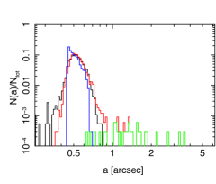
Figure 42.— Size distribution of power-law sources detected with $\theta<2.5^{\prime}$. The histograms include only sources that have src_cnts_aper_b > 25, pileup_warning < 0.01, and (conf_code&0xf) = 0. The black curve shows 1,850 MARX-simulated point sources. The blue curve shows 3,339 SAOSAC-simulated point sources. The red curve shows 3,339 CSC catalog sources; 33 of the selected CSC sources have $a>0.85^{{\prime}{\prime}}$. The green curve shows CSC sources meeting the above criteria that also have (extent_code&0x10) != 0.

Because the MARX and SAOSAC simulators have been tuned to closely approximate the Chandra PSF, we expect close agreement between the point-source size distribution derived from MARX and SAOSAC point-source simulations and the size distribution derived from CSC point sources. Furthermore, any extended sources appearing in the CSC should appear as a tail extending above the point-source size distribution. Such extended sources should also be flagged with one or more non-zero extent_code bits.

Fig. 42 shows the distribution of RSS, $a$, among CSC sources and MARX-  and SAOSAC-simulated point-sources with off-axis angle $\theta\leq 2.5^{\prime}$. The MARX point-source distribution is broader than the SAOSAC point-source distribtion because the MARX simulations sample much fainter sources. In contrast, the SAOSAC sources are uniformly bright because they were created primarily to provide an accurate measure of the PSF size. The close agreement between the simulated point-source size distributions and the observed CSC point-source size distribution confirms the accuracy of the MARX and SAOSAC simulations. A population of apparently extended CSC sources is visible as tail extending to $a\approx 4^{{\prime}{\prime}}$.

A number of b band CSC sources with $\theta\lesssim 2.5^{\prime}$ are marked as extended even though their raw source extent falls within the point source size distribution. For many of these sources, the extent_code bit was set erroneously because, for bright sources with $\theta\lesssim 3.5^{\prime}$, the uncertainty on the source size was underestimated, sometimes falling below $0.1^{{\prime}{\prime}}$. As a result, some point sources were flagged as extended even though the raw source size estimate exceeded the PSF size estimate by $\lesssim 0.1^{{\prime}{\prime}}$. Imposing a minimum source size uncertainty of $0.1^{{\prime}{\prime}}$, 379 CSC sources (81% of which have $\theta<2^{\prime}$ and 98% of which have $\theta<3.5^{\prime}$) would be reclassified from extended to point-source. For $\theta\lesssim 4^{\prime}$, this change in source size uncertainty eliminates most of the overlap between the size distribution of point-sources and the size distribution of sources flagged as extended. We note that many of the affected sources also have (conf_code&0xf) != 0 or pileup_warning$>0.01$, making the extent_code value somewhat questionable for the reasons discussed above.

At off-axis angles $\theta\gtrsim 4^{\prime}$, the CSC source extent distribution appears consistent with that of the MARX-simulated point sources (see Fig. 43), suggesting that few genuinely extended sources appear in the CSC catalog with $\theta>4^{\prime}$. Additional work is in progress to understand this effect.

For off-axis angles $3^{\prime}\leq\theta\lesssim 10^{\prime}$, the point-source size distribution is somewhat bimodal, consisting of a blend of two broad peaks corresponding to sources detected on ACIS-I and on ACIS-S, respectively (see Fig. 43 and Fig. 18 of Evans et al. 2010). The median imaging PSF on ACIS-I is somewhat smaller than the median imaging PSF on ACIS-S because the ACIS-I CCDs are positioned along the imaging focal surface, while the ACIS-S CCDs are positioned along the Rowland torus of HETG.

Figure 43.— Size distribution of power-law sources detected with $3.5^{\prime}<\theta<4.5^{\prime}$. The histograms include only sources that have src_cnts_aper_b > 25, pileup_warning < 0.01, and (conf_code&0xf) = 0. The black curve shows 1,543 MARX-simulated point sources. The red curve shows 2,565 CSC catalog sources. The blue curve shows CSC sources falling on ACIS-S. The green curve shows CSC sources falling on ACIS-I.

11. Variability

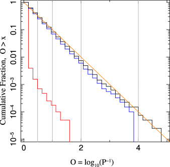
Figure 44.— Cumulative fraction of simulated white noise lightcurves (durations of 160 ksec and mean rates of 0.032 cps) detected with $O\equiv\log_{10}(P^{-1})$ greater than the $x$-axis value. $P$ is the probability that the lightcurve is consistent with a constant lightcurve. Black line (top) is for the Kolmogorov-Smirnov test, blue line (middle) is for the Kuiper test, and red line is for the Gregory-Loredo test (bottom). The straight orange line is $10^{-x}$. Vertical grey lines correspond to the minimum $O$-values for which the CSC variability index (based upon the results of the Gregory-Loredo test) would be set to 5, 6, 7, or 8 (left to right).

Figure 45.— Cumulative fraction of simulated red noise lightcurves (durations of 50 ksec) detected with $O\equiv\log_{10}(P^{-1})$ greater than the $x$-axis value. $P$ is the probability that the lightcurve is consistent with a constant lightcurve. Lightcurves used in the left figure have a mean rate of 0.0032 cps, while those used for the right have a mean rate of 0.032 cps. For each, solid lines are for lightcurves with 30% fractional rms, and dash-dot lines are for 7.5% fractional rms. (Orange lines are $10^{-x}$.) Black lines correspond to the Kolmogorov-Smirnov test, blue lines to the Kuiper test, and red lines to the Gregory-Loredo test.

Figure 46.— Contours for the fraction of simulated red noise lightcurves (as a function of simulated fractional rms and mean count rate) detected as variable with $O\equiv\log_{10}(P^{-1})>2$ (i.e., significantly variable at $>99\%$ confidence). The top row corresponds to the results of the Kuiper test, whereas the bottom row corresponds to the Gregory-Loredo test. From left to right, the durations of the lightcurves were 20 ksec, 50 ksec, and 160 ksec.

As described in Evans et al. (2010), the Chandra Source Catalog utilizes three variability tests: Kolmogorov-Smirnov, Kuiper, and Gregory-Loredo. Results from these tests are stored as a probability, $p$, that the lightcurve in a given band for the indicated variability test is not consistent with being constant (i.e., pure counting noise, modulo source visibility as described by the good time intervals and the time-dependent fraction of the source region that falls on an active portion of the detector). For purposes of characterization, a more useful probability is $P\equiv 1-p$, which can be taken as the probability that a constant lightcurve would have falsely indicated the detected level of variability. It is further convenient to take the negative $\log_{10}$ of this quantity, i.e., define $O\equiv\log_{10}(P^{-1})$. This can be thought of being similar to the log of the odds ratio that a variable lightcurve is a better description than a constant one. (Although the odds ratio is properly a Bayesian concept, and hence applicable only to the Gregory-Loredo test, we define the quantity $O$ for the Kolmogorov-Smirnov and Kuiper tests via their frequentist probabilities $p$ as above so that we can more easily compare results from the three tests.) For much of the characterization work that follows, results are presented in terms of this quantity $O$. Note that even for a “good” variability test, a fraction, $f_{P}$, of lightcurves with a constant mean rate should yield probabilities $P\leq f_{P}$, or equivalently, $O\geq\log_{10}(f_{P}^{-1})$.

We first assess this expected property of the variability tests by applying them to white noise simulations. For pure white noise simulations, at least for the Kolmogorov-Smirnov and Kuiper tests, we expect that the cumulative fraction of lightcurves with $O$ greater than a given value, $x$, will follow $10^{-x}$. Some deviations from this relationship are expected for two reasons: First, we include a simple model of pileup and assume that the pileup parameter $\alpha=0.5$ (i.e., there is a $0.5^{(n-1)}$ probability that $n$ piled events will be detected as a single good event). This will tend to suppress statistical fluctuations for the brighter lightcurves (Davis, 2001). Second, we apply the lower count cutoff used within the catalog by not including any lightcurves with fewer then ten counts, and thus we are suppressing some range of inherent Poisson variability (fluctuations to low counts from lightcurves with mean counts just above the threshold, and fluctuations to high counts from lightcurves with mean counts just below the threshold).

We simulate 40,000 lightcurves at each of seven different lengths ranging from 1 ksec to 160 ksec and 8 different mean rates ranging from 5.6e-4 cps to 3.2e-2 cps, for a total of 2,240,000 simulations. Histograms of the test results for the longest, brightest lightcurves are presented in Fig. 44, although results for lightcurves of different lengths and mean rates are comparable. We find that for the most part, the Kolmogorov-Smirnov and Kuiper tests yield the expected results for the white noise lightcurve. That is, the cumulative fraction of simulated lightcurves with test results indicating variability decreases with the significance level of the results. Given that Fig. 44 represent 40,000 lightcurves, we find as expected $\approx 400$ simulations that (falsely) indicate variability at $\geq 99.9\%$ confidence. Note, however, that the Kolmogorov-Smirnov test and especially the Kuiper test each show a small deficit of lightcurves with high variability significance levels. We attribute this primarily to the effect of pileup on the generated lightcurves. These deficits are small, however, and we find that the usual notion of significance levels applies well to these simulated lightcurves when using the Kolmogorov-Smirnov and Kuiper tests.

The Gregory-Loredo test assigns even fewer white noise lightcurves to formally significant statistic levels. It is important to remember, however, that the Gregory-Loredo test is answering a more restrictive question. Rather than asking the simple question, “Is this lightcurve consistent with a constant rate?”, it is instead asking, “Is a uniformly binned lightcurve with multiple time bins a better description than a single bin, constant rate lightcurve?”. The Gregory-Loredo test, for example, is not well-suited for discovering a single, short flare interspersed in an otherwise steady lightcurve. We find that the Gregory-Loredo test (which, again, is the basis for the CSC tabulated variability indices) yields fewer false positives; however, as we show below, it is also less sensitive to real variability. The Gregory-Loredo test is therefore a somewhat more conservative measure of variability than either the Kolmogorov-Smirnov or Kuiper tests.

We next turn to the question of sensitivity to real lightcurve variability. We simulated red noise lightcurves with the same lengths and mean rates as for the white noise simulations; however, we further considered a range of 12 fractional rms levels, ranging from 1% to 30%. We performed 6,000 simulations for each combination of lightcurve length, mean rate, and fractional rms, yielding a total of 4,032,000 simulations. The cumulative fractions of simulated lightcurves above a given significance threshold, for a subset of simulated lightcurve lengths, rates, and fractional rms values, are shown in Fig. 45. The variability tests performed on these simulations – for lightcurves that are sufficiently bright, long, and/or variable – clearly indicate variability above and beyond the expectations of pure white noise.

To further quantify the meaning of “sufficiently bright, long, and/or variable”, in Fig. 46 we present what essentially amount to “variability detection probability” contours as a function of rms variability ($x$-axis) and mean lightcurve rate ($y$-axis) for a variety of lightcurve lengths (individual panels). For example, here we choose as a “significant” detection threshold a variability test value of $O\geq 2$. The calculated fraction of simulated lightcurves that yield a variability significance above this value is a measure of the sensitivity of the tests for these particular types of lightcurves.

In general we see that the Kuiper test is more sensitive than the Gregory-Loredo test. (The Kolmogorov-Smirnov test yields contours similar to the Kuiper test.) Not unexpectedly, the brighter, more highly variable, and longer the lightcurve, the more sensitive the tests. Ideally, for a set of truly variable, well-observed lightcurves and a chosen threshold for the value of $O=\log_{10}(P^{-1})$, we hope to find that the fraction, $f_{\rm lc}$, of lightcurves exceeding this threshold to be $f_{\rm lc}\gg P=10^{-O}$. For many realistic parameter regimes, however, $<10\%$ of the simulated variable lightcurves are in fact detected as being variable with $O>2$ (or equivalently, $P<10^{-2}$). This is to be borne in mind when considering the catalog results which we discuss below.

Results from applying the variability tests to CSC sources are shown in Fig. 47. Specifically, we show histograms of the variability indices (derived from the Gregory-Loredo test; Evans et al. 2010) in each of the ACIS energy bands used in the catalog. Note that here we have excluded any source that dithers over a chip edge. Of the over 90,000 sources examined, nearly 13% have a maximum variability index $\geq 6$, and nearly 6% have a maximum variability index $\geq 7$. These two variability indices represent, respectively, $>90\%$ and $>99\%$ confidence that the source is better described by a uniformly binned, variable lightcurve rather than by a white noise lightcurve. The b band shows the most highly significant variability detections, most likely due to the increased counting statistics available for this band. Otherwise, detection significance tends to decrease from the hardest h to the softest u bands. This is likely a combination of detector properties (ACIS-I has very little sensitivity in the u band and has reduced sensitivity in the s band compared to ACIS-S), observational properties (e.g., the soft energy bands are easily obscured by interstellar absorption), and intrinsic source properties.

Figure 47.— Histograms of variability results from the CSC, for different energy bands, in terms of the variability index, excluding sources that dither across a chip edge. Orange, red, green, blue, and purple lines represent the u, s, m, h, and b bands, respectively. The thick black line is the maximum variability index from the five bands.

We next turn to the significances as determined by the variability tests. Examining the three different test results in the s, m, h, and b energy bands individually, we find that between 4–16% of the lightcurves have $O\geq 2$, and 1–7% of the lightcurves have $O\geq 3$ (again, roughly corresponding to the $>90\%$ and $>99\%$ confidence levels for significant variability, respectively). Within each energy band, the lower end of the percentage range is for the Gregory-Loredo test (which again, is asking a more stringent question than merely is the lightcurve variable), while for all tests the soft band shows the smallest percentage of significantly variable lightcurves, consistent with the results of the catalog variability indices discussed above.

At the above respective significance levels, we expect that $<10\%$ and $<1\%$ of an ensemble of white noise lightcurves would show comparably significant results. Thus we see that up to approximately 5–6% of the CSC sources (i.e., the excess above the $<1\%$ of sources we expect to have $O>3$) are detected as being truly variable. This is to be compared to, for example, the $<1\%$ of detections (2,307/246,897) classified as variable in the 2XMM catalog (Watson et al., 2009). In practice, for the CSC as a whole a significant population of variable sources begins to appear at variability indices $\geq 5$ and variability test values $O>1$. This is illustrated in Fig. 48, which shows the CSC variability test results for the b band. Here we show the cumulative fraction of sources with $O=\log_{10}(P^{-1})$ greater than a given value for each of the three tests. This is to be compared to the white noise expectation that the curves follow $10^{-x}$. Excesses above this line represent populations of significantly variable sources.

Figure 48.— Cumulative fraction of sources from the CSC (excluding sources that dither across a chip edge) that exceed a given variability significance (expressed as $O=\log_{10}(P^{-1})=-\log_{10}(1-p)$) for the three variability tests performed in the (b) band. Black histogram (top) is for the Kolmogorov-Smirnov test, blue histogram (middle) is for the Kuiper test, and red histogram (bottom) is for the Gregory-Loredo test. The orange straight line is the expectation for constant rate lightcurves, subject only to Poisson noise. The grey vertical lines are the boundaries for the catalog variability indices (based upon the Gregory-Loredo test) 5, 6, and 7.

In practice, one would identify variability in a subset of catalog sources by choosing a threshold value of $O$. Sources with $O$ exceeding this threshold would be identified as variable. A low threshold would yield a larger number of variable sources, but also a larger fraction of “false positives”. On the other hand, choosing very high test significances for the threshold will reduce the number of flagged sources. For the catalog as a whole, choosing $O\geq 2$ in either the Kolmogorov-Smirnov or Kuiper test, or nearly equivalently a variability index $\geq 7$, maximizes the difference between the cumulative histograms for the detected and white noise significances. Approximately 6% of the sources will be flagged as variable, of which $\approx 17\%$ are likely false positives (i.e., 1/6, as we expect 1% of non-variable sources to achieve such high test significance values). Given that the Kolmogorov-Smirnov and Kuiper tests have very well-characterized properties for white noise lightcurves, those test results can be used as a guide for assessing variability in any sub-populations taken from the catalog. Those tests specifically should allow users to choose their own optimization of number of variable sources vs. fraction of false positives. The Gregory-Loredo test, having less well-characterized white noise properties, is less well-suited for that task; however, its chief advantage lies in the fact that it also provides an estimate of the lightcurve which can be used in more sophisticated analyses.

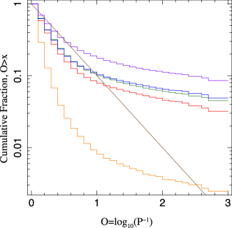
Figure 49.— Cumulative fraction of CSC v.1.0.1 master sources (comprised of two or more individual observations) detected with inter-observation variability above a given value of $O\equiv\log_{10}(P^{-1})$, greater than the $x$-axis value. Bottom line (orange) is for the u band, followed by the s (red), m (green), h (blue), and b (purple) bands. The straight line (brown) is $10^{-x}$, and again is the expectation for random noise fluctuations.

We separately have analyzed the variability from catalog sources that dither over a chip edge (by selecting the approximately 38,000 sources with edge_code or multi_chip_code $>0$). To minimize issues arising from the programming error related to sources dithering onto an off or excluded chip, we did not include any sources from ObsIDs with an excluded chip. (A list of such ObsIds is maintained on the CSC website.) The results are very similar to the above. 17% of those sources have a maximum variability index $\geq 6$, and 7% have a maximum variability index $\geq 7$. Examining the three different test results in four energy bands separately, we find that between 5–17% of the lightcurves have $O\geq 2$, and 2–7% of the lightcurves have $O\geq 3$. These percentages are slightly higher than those quoted above, but not dramatically so. There is likely some additional false variability associated with dithering over the edge, but this does not dominate the results from these sources if one choose a test threshold of $O=2$.

Although we have not performed simulations to assess the sensitivity of our procedures for detecting inter-observation variability, as for the intra-observation variability tests discussed above we have conducted a preliminary assessment of the actual CSC v.1.0.1 results. The CSC includes master source variability probabilities, var_inter_prob_*, that represent the probability that the multiple observations that comprise a given master source are not consistent with a constant flux in a given energy band. To be consistent with our prior discussion of intra-observation variability, we again convert these probabilities, $p$, into a quantity similar to a logarithmic odds ratio, $O\equiv\log_{10}(1-p)$. We again consider the cumulative fraction of sources above a given value, $O$. Again, even for non-varying sources, we expect by random noise for 10% to have $O\geq 1$, 1% to have $O\geq 2$, etc. Results for master sources comprised of two or more individual observations are presented in Fig. 49.

The selection of master sources comprised of two or more individual observations (necessary for the definition of inter-observation variability) limits the selection to 17,538 unique master source IDs. It should be noted, however, that although there are multiple observations for each of these master sources, each energy band is not necessarily significantly detected in each individual observation. This is reflected in Fig. 49, where the u band is seen to be skewed towards extremely low inter-observation variability significance. This is unsurprising as the u band flux might have been significantly detected in an ACIS-S observation, yet remain undetected in an ACIS-I observation. In general, we see that the harder bands, and especially the b band, follow more closely the expected $10^{-x}$ behavior for low values of $O$.

We see, however, that all energy bands show a tail of larger $O$ values that represent the significant detection of inter-observation variability. This tail is most pronounced for the b band, where $\approx 20\%$ of sources have $O\geq 1$, and 10% of sources have $O\geq 2$. Thus, approximately 10% of all master sources comprised of multiple observations show significant inter-observation variability. Furthermore, choosing a selection critereon of var_inter_prob$\geq 0.99$ identifies these sources, with only $\lesssim 10\%$ of them being “false positives”.

12. Conclusions

The Chandra Source Catalog is intended to be a general resource for astronomers at all wavelengths. It differs from the many excellent Chandra catalogs derived as part of specific scientific programs in that its data selection and analysis procedures are not optimized for any particular scientific goal. With few exceptions, data from all detectors active in each observation are included, and data from all observations are processed in a uniform manner with a uniformly defined set of source properties. The statistical characterization studies we present here are based on extensive simulations and comparisons to other catalogs, and illuminate the differences between the CSC and other Chandra catalogs.

The first release of the Chandra Source Catalog includes a large fraction of all Chandra ACIS non-grating observations made in the first eight years of the Chandra mission. Significant characterization results include the following.

• The catalog contains $\sim 94,700$ distinct X-ray sources from $\sim 3,900$ separate ACIS observations.

• The total sky coverage is $\sim 320$ deg.² for sources with a 0.5–7.0 keV photon flux greater than $\sim 4\times 10^{-5}$ ph cm^-2 s^-1.

• Detection efficiencies are:

  • typically near $\sim 100$% for sources within $\sim 5^{\prime}$ of the aimpoint and brighter than $\sim 1$–$3\times 10^{-6}$ ph cm^-2 s^-1, depending on exposure, and

  • $\sim 50$% or better for sources between $\sim 5$–$10^{\prime}$ off axis.

• False source detections appear to cluster near chip edges and the boundaries between back- and front-illuminated chips, but the false source rate is appreciable only for observations with exposures longer than $\sim$50 ksec.

• Fewer than $\sim 1$% of the sources in the CSC are spurious.

• Average positional errors of CSC sources range from $\sim 0.2^{{\prime}{\prime}}$ on-axis to $\sim 4^{{\prime}{\prime}}$ at $\sim 14^{\prime}$ off-axis.

• Systematic errors in photon fluxes inlcude an overestimate of a factor of $\lesssim 2$ for sources fainter than $\sim 3\times 10^{-6}$ ph cm^-2 s^-1 and at off-axis angles $\theta\gtrsim 10^{\prime}$, due at least in part to an uncorrected Eddington bias when detection efficiency is low. Additional systematic errors at higher fluxes include both underestimates and overestimates of $\sim 10-30\%$, depending on energy band and source spectrum, and are attributed to the use of a monochromatic effective area in computing fluxes. Systematic errors in u band fluxes can be $\gtrsim 30\%$, for some source spectra.

• Extended sources with sizes of a few arcseconds can be detected within $\sim 2.5^{\prime}$ of observation aimpoints; further work is required to fully characterize CSC extent capabilities farther off-axis.

• Choosing a 99% confidence level for source variability (using either the Kuiper or Kolmogorov-Smirnov tests), 6% of all CSC sources are found to be significantly variable. Less than 1/6 of these detections are expected to be false positives.

• Approximately 10% of all master sources comprised of multiple observations show significant inter-observation variability. Less than 10% of these detections are expected to be false positives.

Results presented here apply to the Release 1.0.1 of the Chandra Source Catalog. However, they should also apply to ACIS CSC sources in incremental Release 1.1, which was made public in August, 2010. ACIS analysis procedures do not, in general, differ between releases 1.0.1 and 1.1. The latter does, however, include HRC-I data, and although HRC-I analysis procedures are not different, its different detector characteristics merit additional characterization. Additional HRC-I characterization results will be presented when available.

Appendix A A Comparison of the MARX and SAOTrace PSFs

Figure 50.— The ACIS-I encircled energy radius at the 10, 50, 90, and 95 percent levels as a function of off-axis angle for various energies

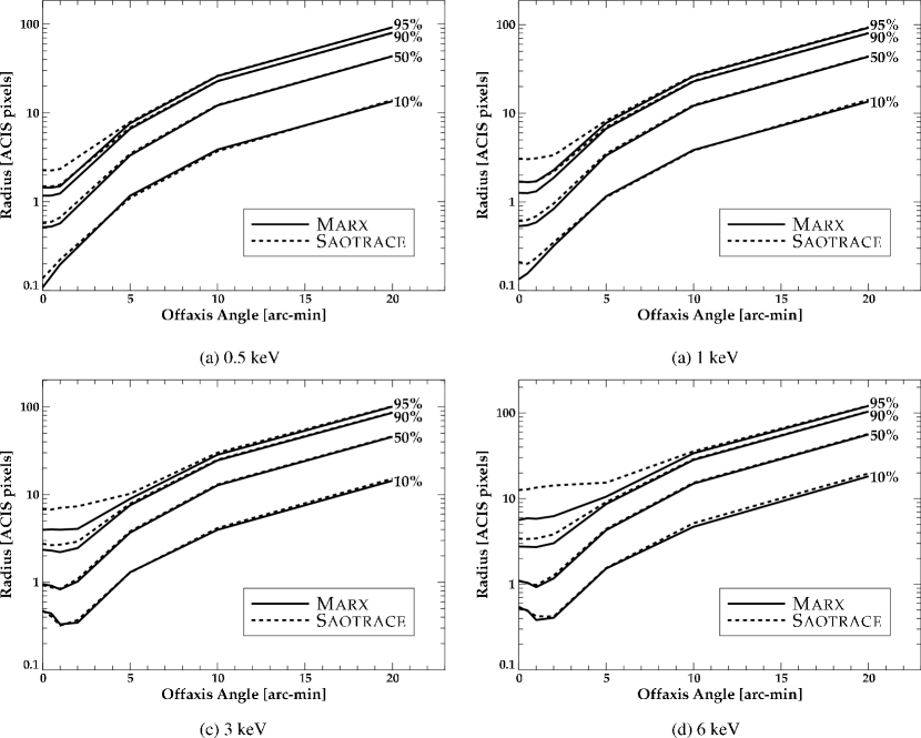
Figure 51.— The ACIS-S encircled energy radius at the 10, 50, 90, and 95 percent levels as a function of off-axis angle for various energies.

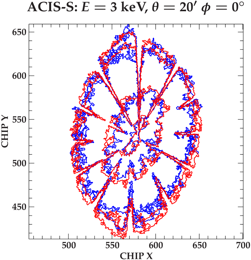
Figure 52.— The 10, 50, 90, and 95 percent MARX (blue) and SAOTrace (red, or halftone) encircled energy contours for a 3 keV source 20’ off-axis on ACIS-S.

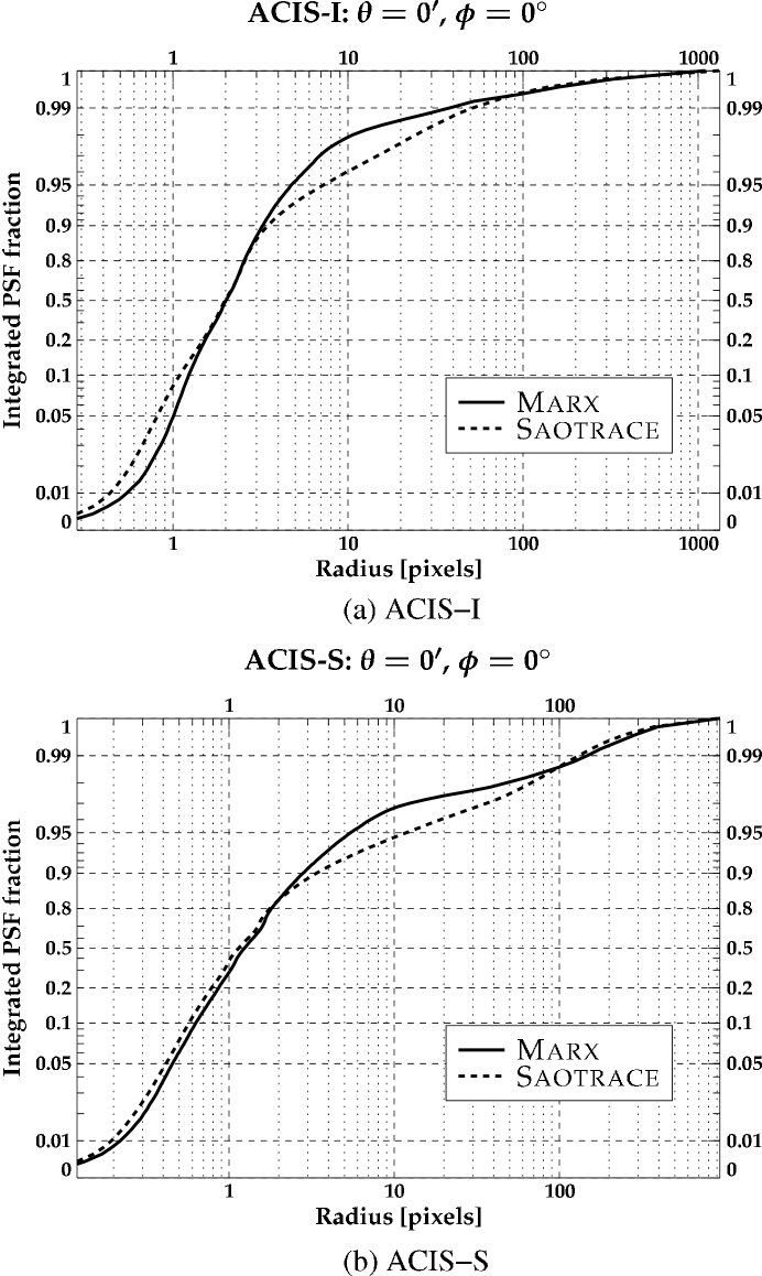
Figure 53.— The encircled energy as a function of radius for an on-axis source on the ACIS-I and ACIS-S arrays. The source spectrum was assumed to be an absorbed powerlaw with an absorbing column of $10^{21}$ cm^-2 and index of $1.7$.

MARX (Model of AXAF response to X-rays) is a suite of programs designed to simulate the on-orbit response of the Chandra X-ray Observatory. It was used for release 1.0.1 of the catalog to characterize the detection efficiency, flux accuracy, and relative astrometry via point sources simulated at various off-axis angles, energies, and instrument configurations. To better understand the accuracy of the characterization, it is important to know how well the MARX Point Spread Function (PSF) approximates that of the telescope. It is far beyond the scope of this work to make a direct comparison of the simulated MARX PSF to that of actual flight data. Instead, we compare the MARX PSF to that of the high-fidelity High Resolution Mirror Assembly (HRMA) ray-trace program SAOTrace, which has undergone extensive pre-flight and post-flight calibration.

The shape of the observed PSF is a complicated non-linear function that depends upon a number of variables including off-axis angle, energy, instrument configuration, detection mode, and source flux. Since incident photons first interact with the Chandra HRMA before arriving at the detector, the observed PSF is a convolution of a HRMA PSF and detector PSF. The detector PSF consists of an astigmatic component caused by deviations of the detector geometry from that of the ideal focal surface, a component due to the use of finite size detector pixels, and an intrinsic component that arises from the interaction of the photon with the detector. With the exception of the latter, the former two components are purely geometrical and are handled in a straight forward manner by the MARX raytrace. Positional uncertainties from the physical interaction of the photon with the detector are handled statistically by assuming an additional gaussian blur when MARX constructs event coordinates.

The HRMA PSF may be broken into two parts. The first is a component that dominates the core of the PSF and is a consequence of misalignments and low spatial frequency deviations from the perfect type-I Wolter geometry. The second part gives rise to the scattering wings of the PSF and is caused by high frequency surface errors or microroughness. In principle, given a detailed geometric model of the mirror, the core of the PSF could be simulated via ray-tracing. However, MARX lacks the detailed geometric details of the HRMA but instead assumes perfect type-I Wolter geometry for each of the mirror shells and takes into account misalignments between them. MARX models the low spatial frequency deviations from the ideal Wolter-I geometry by rotating the surface normal at the intersection point of a ray about a random direction perpendicular to the normal by a small angle chosen from a gaussian distribution. The scattering wings of the HRMA PSF are treated statistically by MARX using a parametrization developed by van Speybroeck et al. (1989) of the Beckmann & Spizzichino (1963) scattering model.

The encircled energies of the MARX and SAOTrace ACIS-I PSFs as a function of off-axis angle at various energies are shown in Fig. 50; the corresponding PSFs for ACIS-S are depicted in Fig. 51. From these plots one can see that beyond about $5^{\prime}$ off-axis, the MARX and SAOTrace PSFs agree quite well. This agreement can also be seen in Fig. 52, which shows 2d encircled energy contours for a $20^{\prime}$ off-axis source. Fig. 53 shows that on-axis, the encircled energies of the MARX and SAOTrace PSFs agree out to about 90 percent of the integrated flux, but differ in the scattering wings.

The fact that the MARX and SAOTrace PSFs agree far off-axis, but disagree near on-axis in the wings should not be surprising. The various statistical parameters that MARX uses to characterize the PSF were tuned to match the High Efficiency Transmission Grating Spectrometer’s (HETGS) on-axis Line Spread Function (LSF) as determined through HETGS observations of Capella (Canizares et al., 2005). Due to the lack of adequate counts in the wings of the LSF, only the parameters influencing the PSF core could be determined with sufficient resolution. The use of the HETGS for this purpose is a reflection of the fact that MARX started out as a simulator for the HETGS. In contrast, the on-axis SAOTrace PSF was compared to HRC-I observations of Ar-Lac Jerius, Gaetz & Karovska (2004), where the residuals in the core of PSF were estimated to be less than 10 percent. The wings of the SAOTrace PSF were accessed using the zeroth order HETGS data from a 50 ksec observation of Her X-1. From this observation, the uncertainties in the flux of the SAOTrace wings were estimated to be at least 30–50% (see the discussion of Xiang, Lee & Nowak, 2009).

For near on-axis sources, the relative positional accuracy in the sky tangent plane system between the MARX and SAOTrace PSFs was determined by comparing the tangent plane locations of the centroids of their PSFs. For such cases, we found MARX to be consistent with SAOTrace to subpixel accuracy.

Centroiding was less useful for far off-axis sources where the distortions in the core of the PSF become quite noticeable. In this situation, the intersection of the shadows caused by the HRMA support struts as seen in the sky tangent plane coordinate system was used to determine the source position. The astigmatic effects associated with the different path lengths of rays from the HRMA to the detector surface mean that the strut shadows may not have a common intersection point in the sky and detector coordinate systems. This is particularly noticeable for the ACIS-S detector planes, which were designed to approximate the Rowland surface of the HETGS causing them to be offset from the imaging focal surface. The accuracy of this method was estimated to be less than 2 arc-seconds for sources 25 arc-minutes off-axis.

The previous technique was used to compare the MARX PSF to that of the Chandra observation (OBSID 1068) of LMC X-1, observed 24.8 arc-minutes off-axis. A Level 2 event file was created using CIAO 4.2 and loaded into SAOImage ds9 Joye & Mandel (2003) to view the (binned) source events in the sky tangent plane system. Using the intersection of the strut shadows as described above, the source was estimated to have a right ascension of 84.9115$\pm$0.0002 degrees and a declination of -69.74335$\pm$0.00028 degrees. These values were used to to specify the source position for a MARX point source simulation of OBSID 1068. The resulting MARX event file and the Chandra observation level 2 event file were loaded into SAOImage ds9 to visually compare the observed and simulated PSFs by “blinking” one against the other. As expected, qualitative differences were seen in the core of the PSF but the positions of the support strut shadows were nearly on top of one another with a registration uncertainty estimated to be less than two sky tangent plane pixels, which is consistent with the uncertainties in the source position estimated using the support struts.

References

- Abazajian et al. (2009) Abazajian, K. N., et al., 2009, ApJS, 182, 543
- Alexander et al. (2003) Alexander, D. M., et al., 2003, AJ, 126, 539
- Beckmann & Spizzichino (1963) Beckmann, P., & Spizzichino, A., 1963, Scattering of Electromagnetic Waves from Rough Surfaces, (New York: Pergamon Press), first edition
- Brandt et al. (2001) Brandt, W. N., et al., 2001, AJ, 122, 2810
- Brinkman et al. (2000) Brinkman, B. C., et al., 2000, in Society of Photo-Optical Instrumentation Engineers (SPIE) Conference Series, ed. J. E. Truemper & B. Aschenbach, Vol. 4012, 81
- Budavári & Szalay (2008) Budavári, T., & Szalay, A. S., 2008, ApJ, 679, 301
- Canizares et al. (2005) Canizares, C. R., et al., 2005, PASP, 117, 1144
- Davies & Harte (1987) Davies, R., & Harte, D., 1987, Biometrica, 3, 95
- Davis (2001) Davis, J. E., 2001, ApJ, 562, 575
- Doe et al. (2007) Doe, S., et al., 2007, in Astronomical Data Analysis Software and Systems XVI, ed. R. A. Shaw, F. Hill, & D. J. Bell, Vol. 376, 543
- Eddington (1940) Eddington, Sir, A. S., 1940, MNRAS, 100, 354
- Evans et al. (2010) Evans, I. N., et al., 2010, ApJS, 189, 37
- Freeman, Doe & Siemiginowska (2001) Freeman, P., Doe, S., & Siemiginowska, A., 2001, in Society of Photo-Optical Instrumentation Engineers (SPIE) Conference Series, ed. J.-L. Starck & F. D. Murtagh, Vol. 4477, 76
- Garmire et al. (2003) Garmire, G. P., Bautz, M. W., Ford, P. G., Nousek, J. A., & Ricker, Jr., G. R., 2003, in Society of Photo-Optical Instrumentation Engineers (SPIE) Conference Series, ed. J. E. Truemper & H. D. Tananbaum, Vol. 4851, 28
- Getman et al. (2005) Getman, K. V., et al., 2005, ApJ Suppl., 160, 319
- Giacconi et al. (2002) Giacconi, R., et al., 2002, ApJ Suppl., 139, 369
- Gioia et al. (1990) Gioia, I. M., Maccacaro, T., Schild, R. E., Wolter, A., Stocke, J. T., Morris, S. L., & Henry, J. P., 1990, ApJ Suppl., 72, 567
- Górski et al. (2005) Górski, K. M., Hivon, E., Banday, A. J., Wandelt, B. D., Hansen, F. K., Reinecke, M., & Bartelman, M., 2005, ApJ, 622, 759
- Gregory & Loredo (1992) Gregory, P. C., & Loredo, T. J., 1992, ApJ, 398, 146
- Houck & Denicola (2000) Houck, J. C., & Denicola, L. A., 2000, in ASP Conf. Ser. 216: Astronomical Data Analysis Software and Systems IX, Vol. 9, 591
- Jerius, Gaetz & Karovska (2004) Jerius, D. H., Gaetz, T. J., & Karovska, M., 2004, in Society of Photo-Optical Instrumentation Engineers (SPIE) Conference Series, ed. K. A. Flanagan & O. H. W. Siegmund, Vol. 5165, 433
- Joye & Mandel (2003) Joye, W. A., & Mandel, E., 2003, in Astronomical Data Analysis Software and Systems XII, ed. H. E. Payne, R. I. Jedrzejewski, & R. N. Hook, Vol. 295, 489
- Kim et al. (2004a) Kim, D., et al., 2004a, ApJ Suppl., 150, 19
- Kim et al. (2004b) Kim, D., et al., 2004b, ApJ, 600, 59
- Kim et al. (2007) Kim, M., et al., 2007, ApJS, 169, 401
- Kuiper (1960) Kuiper, N. H., 1960, Indagationes Mathematicae, 22, 38
- Laird et al. (2009) Laird, E. S., et al., 2009, ApJS, 180, 102
- Luo et al. (2008) Luo, B., et al., 2008, ApJ Suppl., 179, 19
- Murray et al. (2000) Murray, S. S., et al., 2000, in Society of Photo-Optical Instrumentation Engineers (SPIE) Conference Series, ed. J. E. Truemper & B. Aschenbach, Vol. 4012, 68
- Park et al. (2006) Park, T., Kashyap, V. L. andSiemiginowska, A., van Dyk, D. A., Zezas, A., Heinke, C., & Wargelin, B. J., 2006, ApJ, 652, 610
- Pier et al. (2003) Pier, J. R., Munn, J. A., Hindsley, R. B., Hennessy, G. S., Kent, S. M., Lupton, R. H., & Ivezić, Ž., 2003, AJ, 125, 1559
- Press et al. (2007) Press, W. H., Teukolsky, S. A., Vetterling, W. T., & Flannery, B. P., 2007, Numerical Recipes: the Art of Scientific Computing, (Cambridge: Cambridge University Press), third edition
- Stephens (1974) Stephens, M., 1974, Journal of the American Statistical Association, 69, 730
- Timmer & Koenig (1995) Timmer, J., & Koenig, M., 1995, A&A, 300, 707
- Ueda et al. (2005) Ueda, Y., Ishisaki, Y., Takahashi, T., Makishima, K., & Ohashi, T., 2005, ApJ Suppl., 161, 185
- van Speybroeck et al. (1989) van Speybroeck, L., Scwartz, D., Reid, P., & Bilbro, J., 1989, Vol. 1160, 94
- Vaughan & Uttley (2007) Vaughan, S., & Uttley, P., 2007, in “Noise and Fluctuations”, Proceedings of the SPIE, Volume 6603, ed. L. Cohen, 660314
- Voges et al. (1999) Voges, W., et al., 1999, A&A, 349, 389
- Voges et al. (2000) Voges, W., et al., 2000, IAU Circ. 6100
- Watson et al. (2009) Watson, M. G., et al., 2009, A&A, 493, 339
- Weisskopf et al. (2002) Weisskopf, M. C., Brinkman, B., Canizares, C., Garmire, G., Murray, S., & Van Speybroeck, L. P., 2002, PASP, 114, 1
- White, Giommi & Angelini (1994) White, N. E., Giommi, P., & Angelini, L., 1994, IAU Circ. 6100
- Xiang, Lee & Nowak (2009) Xiang, J., Lee, J. C., & Nowak, M. A., 2009, ApJ, 660, 1309