Casimir repulsion in moving media

Abstract

Casimir-Lifshitz interaction emerging from relative movement of layers in stratified dielectric media (e.g., non-uniformly moving fluids) is considered. It is shown that such movement may result in a repulsive Casimir-Lifshitz force exerted on the layers, with the simplest possible structure consisting of three adjacent layers of the same dielectric medium, where the middle one is stationary and the other two are sliding along a direction parallel to the interfaces of the layers.

I Introduction

In this paper we consider Casimir-Lifshitz forces Casimir (1948); Lifshitz (1956) in layered moving media. Our interest to this problem was initiated by a recent discussion on the friction forces that may or may not appear due to quantum-electromagnetic fluctuations in systems involving moving dielectric slabs Philbin and Leonhardt (2009); Pendry (2010a); Leonhardt (2010); Pendry (2010b); Barton (2010); Høye and Brevik (2010). In this paper, however, we will concentrate on another interesting theoretical issue which, to the best of our knowledge, has not been addressed so far: on the possibility of having repulsive Casimir-Lifshitz forces in moving dielectrics. The so-called Casimir repulsion is known to appear between electrically and magnetically polarizable objects in vacuum Boyer (1974); Santos et al. (1999); Kenneth et al. (2002); Rosa and Lambrecht (2010), or between dielectric objects of different permittivity that are immersed in a dielectric fluid of an intermediate permittivity Dzyaloshinski et al. (1965); Munday et al. (2009); Rahi and Zaheer (2010). Very recently, ultralong-range repulsive forces in piston configurations involving cut metallic nanorods have been reported Maslovski and Silveirinha (2011). There have been also attempts on achieving repulsion or “quantum levitation” with the use of other metamaterials Henkel and Joulain (2005); Leonhardt and Philbin (2007); Pirozhenko and Lambrecht (2008); Rosa et al. (2008); Rosa (2009); Yannopapas and Vitanov (2009); Zhao et al. (2009, 2010). However, recently it has been shown that the force between metal-dielectric metamaterial slabs in vacuum is always attractive Silveirinha (2010); Silveirinha and Maslovski (2010a, b). The symmetry considerations also impose restrictions on the sign of the Casimir force Kenneth and Klich (2006); Rahi et al. (2010).

In this paper we are going to consider the case in which the force appears only as the result of relative movement of dielectric layers. In contrast to the Casimir friction studies, we are interested in the force component perpendicular to the direction of the movement. The main idea of this work is to consider a system which is initially balanced, i.e., when there is no movement there are no fluctuation-induced forces. One example of a system with such property is a uniform medium, say a fluid, which is initially at rest. There is, however, a possibility that when separate layers of a fluid begin to slide one with respect to another the balance is destroyed and there appears a noncompensated attractive or repulsive interaction between the sliding layers. It should be well understood at this point that the situation that we consider in this paper differs principally from the previously studied case of moving dielectric slabs separated by a vacuum Philbin and Leonhardt (2009); Pendry (2010a). In the latter case, with an appropriate Lorentz transformation for the electromagnetic field, one may always reduce a problem involving a moving slab of an isotropic dielectric in vacuum to an equivalent problem with a stationary slab of the same isotropic dielectric in vacuum. This is possible because under a Lorentz boost the vacuum “background” remains itself. Quite differently, in this paper we study the Casimir-Lifshitz interactions that appear in non-uniformly moving matter. Applying Lorentz transformations in this case results in a more difficult problem involving layers of anisotropic and nonreciprocal media.

Therefore, we are going to approach this problem without resorting to an assumption that the available theories Casimir and Polder (1948); Casimir (1948); Lifshitz (1956); Kampen et al. (1968) of the Casimir-Lifshitz forces in dielectrics are also applicable in the case of moving media. Instead, we quantize the electromagnetic field in moving matter and derive a relation for the zero-point energy from the first principles. This is required because moving media are not invariant under time reversal and the traditional quantization scheme based on a modal expansion in a large box is not applicable (at least, without significant modifications). In fact, in this work we develop an alternative quantization approach that allows to reuse many of the results of the classic treatment of such nonreciprocal media. Nevertheless, the results of our method fully agree with the phenomenological quantization schemes developed by other authors Jauch and Watson (1948); Kong (1970); Matloob (2005).

The nonreciprocity considered in this paper is twofold: it may either be a result of relativistic movements of material fluids or it may manifest itself in uniaxial bianisotropic metamaterials the constitutive relations of which include a term that is responsible for nonreciprocal magnetoelectric coupling. Such metamaterials have been theoretically known for a long time Kamenetskii (1997); Tretyakov et al. (1998, 2008); certain practical realizations have been proposed as well Tretyakov and Nefedov (2009). Some authors do not make a clear distinction between the real moving media and their metamaterial counterparts, taking for granted that the two types can be described with the constitutive relations of the same form. This is, however, not entirely true. Although applying the Lorentz transformations to the Maxwell equations written for a moving dielectric results (in the laboratory frame) in bianisotropic material relations with nonreciprocal magnetoelectric coupling, such a transformation may not always lead to spatially local constitutive relations. Indeed, the Lorentz transformation intermixes the spatial coordinates with time, therefore, a medium which is nonlocal in time in one of the reference frames (i.e., a dispersive dielectric in its proper frame) becomes nonlocal in both space and time in another reference frame. Thus, a moving dispersive dielectric may be described (in the laboratory frame) with the equivalent spatially local bianisotropic material relations only in a limited frequency range where the dispersion is negligible.

Therefore, in this work the emphasis is mostly on weakly dispersive moving magnetodielectrics for which one may assume that $\varepsilon(\omega)$ and $\mu(\omega)$ are practically constant and real in a wide range of frequencies. This simplification, however, is not crucial for the main theoretical prediction of this paper, namely, the existence of repulsive Casimir-Lifshitz forces in layered moving media. This can be seen from the known fact (see, e.g. Rosa et al. (2008)) that the range of frequencies that make the dominant contribution to the Casimir energy in a pair of material layers separated by the distance $d$ is limited by $|\omega_{\rm max}|\approx 2\pi v_{\rm ph}/d$, where $v_{\rm ph}$ is the phase velocity in the background material. Thus, if $\omega_{\rm max}$ is set to the upper boundary of the region of low dispersion of a medium, then the theory developed in this paper will apply at separations $d\gtrsim 2\pi v_{\rm ph}/|\omega_{\rm max}|$. As there exist real materials with low dispersion and loss up to, at least, the ultraviolet band, the applicability range of our theory may start at hundreds of nanometers. A straightforward generalization of the theory to the dispersive case is outlined in one of the appendices.

The paper is organized as follows. In Section II we solve classically for the eigenwaves in a moving nondispersive medium and discuss their properties. In Section III we derive an expression for the Hamiltonian of the free electromagnetic field in a moving medium and prove an orthogonality relation that holds for the eigenmodes in such a nonreciprocal medium. In Section IV we quantize the (macroscopic) electromagnetic fields in a moving medium and express the Hamiltonian of the electromagnetic field in terms of the creation and annihilation operators of a bosonic field. In Section V we obtain an expression for the zero-point energy and its regular part that represents the Casimir-Lifshitz interaction energy. In Section VI we solve for the Casimir-Lifshitz force in layered moving media. In Section VII we present and discuss some numerical results that clearly demonstrate existence of repulsive Casimir-Lifshitz forces in such media.

II Electromagnetic waves in a moving medium

We consider a uniaxial medium (the axis is along ${\bf z}_{0}$) which is characterized by material relations of the following form [in this section we work in the frequency domain; the time dependence is of the form $\exp(-i\omega t)$]:

$${\bf D} =\overline{\overline{\varepsilon}}\cdot{\bf E}+a{\bf z}_{0}\times{\bf H},$$ (1)

$${\bf B} =\overline{\overline{\mu}}\cdot{\bf H}-a{\bf z}_{0}\times{\bf E},$$ (2)

where $\overline{\overline{\varepsilon}}=\varepsilon_{\rm t}\overline{\overline{I}}_{\rm t}+\varepsilon{\bf z}_{0}{\bf z}_{0}$ and $\overline{\overline{\mu}}=\mu_{\rm t}\overline{\overline{I}}_{\rm t}+\mu{\bf z}_{0}{\bf z}_{0}$ are the dyadic permittivity and the permeability, respectively, with $\overline{\overline{I}}_{\rm t}$ being the unity dyadic in the plane transversal to ${\bf z}_{0}$, and $a$ is the parameter of magnetoelectric coupling. Notice that due to the choice of signs in (1)–(2) this coupling in nonreciprocal.

Such a medium can be envisioned either as a metamaterial with nonreciprocal bianisotropic inclusions, or as a an effective medium resulting from application of the Lorentz transformations to the electromagnetic fields in a magnetodielectric moving with certain velocity $v$ along the $z$-axis. In the latter case, the material parameters as seen in the stationary frame satisfy (see, e.g., Pauli (1958))

$$\varepsilon_{\rm t} =\varepsilon{1-\beta^{2}\over 1-n^{2}\beta^{2}},$$ (3)

$$\mu_{\rm t} =\mu{1-\beta^{2}\over 1-n^{2}\beta^{2}},$$ (4)

$$a ={\beta\over c}{n^{2}-1\over 1-n^{2}\beta^{2}},$$ (5)

where $\varepsilon$ and $\mu$ are the permittivity and the permeability in the comoving frame, $c=1/\sqrt{\varepsilon_{0}\mu_{0}}$ is the speed of light in vacuum, $\beta=v/c$, and $n^{2}=\varepsilon\mu/(\varepsilon_{0}\mu_{0})$. The material parameters are assumed nondispersive and lossless in (3)–(5), but, in fact, these relations may be also generalized for dispersive moving media if plane waves are considered (this is further discussed in Appendix C).

It should be noted that when these transformations are applied to a medium with $n^{2}=1$, they result in $a=0$ and the old values of the permittivity and permeability, independently of the velocity $v$. Thus, due to (3)–(5), a vacuum appears as a “medium” with properties invariant with respect to relative motion, while media with nontrivial refractive index are seen differently in different inertial frames of reference.

The Maxwell equations for the fields in a moving medium can be written as

$$i\omega\overline{\overline{\mu}}\cdot{\bf H} =\nabla_{\rm t}\times{\bf E}+(i\omega a+{\partial_{z}}){\bf z}_{0}\times{\bf E},$$ (6)

$$-i\omega\overline{\overline{\varepsilon}}\cdot{\bf E} =\nabla_{\rm t}\times{\bf H}+(i\omega a+{\partial_{z}}){\bf z}_{0}\times{\bf H},$$ (7)

where $\nabla_{\rm t}\equiv\overline{\overline{I}}_{\rm t}\cdot\nabla$ and $\partial_{z}\equiv\partial/\partial z$. Seeking for plane wave solutions of (6)–(7), it is possible to reduce Eqs. (6)–(7) to

$$\left[\omega^{2}\varepsilon_{\rm t}\mu_{\rm t}-(k_{z}+\omega a)^{2}-{\varepsilon_{\rm t}\over\varepsilon}k_{\rm t}^{2}\right]E_{z} =0,\quad(\mbox{TM}_{z}),$$ (8)

$$\left[\omega^{2}\varepsilon_{\rm t}\mu_{\rm t}-(k_{z}+\omega a)^{2}-{\mu_{\rm t}\over\mu}k_{\rm t}^{2}\right]H_{z} =0,\quad(\mbox{TE}_{z}),$$ (9)

where ${\bf k}={\bf k}_{\rm t}+k_{z}{\bf z}_{0}{\bf z}_{0}$, ${\bf k}_{\rm t}\equiv\overline{\overline{I}}_{\rm t}\cdot{\bf k}$, is the wave vector of a plane wave, and the two equations (8) and (9) are for two independent polarizations: the transverse magnetic polarization with respect to the $z$-axis (TM_z), for which $H_{z}\equiv 0$, and the transverse electric polarization (TE_z), for which $E_{z}\equiv 0$. The transversal components of the electric and magnetic fields (with respect to the $z$-axis) in both TM_z and TE_z polarizations can be expressed through the $z$-components of the fields:

$${\bf H}_{\rm t}^{\rm TM_{z}} ={\omega\varepsilon({\bf k}_{\rm t}\times{\bf z}_{0})\over k_{\rm t}^{2}}E_{z},\quad{\bf E}_{\rm t}^{\rm TM_{z}}=-{\varepsilon(k_{z}+\omega a){\bf k}_{\rm t}\over\varepsilon_{\rm t}k_{\rm t}^{2}}E_{z},\quad (\mbox{TM}_{z}),$$ (10)

$${\bf E}_{\rm t}^{\rm TE_{z}} =-{\omega\mu({\bf k}_{\rm t}\times{\bf z}_{0})\over k_{\rm t}^{2}}H_{z},\quad{\bf H}_{\rm t}^{\rm TE_{z}}=-{\mu(k_{z}+\omega a){\bf k}_{\rm t}\over\mu_{\rm t}k_{\rm t}^{2}}H_{z},\quad (\mbox{TE}_{z}).$$ (11)

The electric displacement ${\bf D}$ and the magnetic induction ${\bf B}$ in the same modes can be found with the help of the material relations (1)–(2) and the relations (10)–(11):

$$\begin{split}{\bf B}_{\rm t}^{\rm TM_{z}}&={\varepsilon((\varepsilon_{\rm t}\mu_{\rm t}-a^{2})\omega-ak_{z})({\bf k}_{\rm t}\times{\bf z}_{0})\over\varepsilon_{\rm t}k_{\rm t}^{2}}E_{z},\quad B_{z}^{\rm TM_{z}}=0,\\ {\bf D}_{\rm t}^{\rm TM_{z}}&=-{\varepsilon k_{z}{\bf k}_{\rm t}\over k_{\rm t}^{2}}E_{z},\quad D_{z}^{\rm TM_{z}}=\varepsilon E_{z},\end{split}\quad (\mbox{TM}_{z}),$$ (12)

$$\begin{split}{\bf D}_{\rm t}^{\rm TE_{z}}&=-{\mu((\varepsilon_{\rm t}\mu_{\rm t}-a^{2})\omega-ak_{z})({\bf k}_{\rm t}\times{\bf z}_{0})\over\mu_{\rm t}k_{\rm t}^{2}}H_{z},\quad D_{z}^{\rm TE_{z}}=0,\\ {\bf B}_{\rm t}^{\rm TE_{z}}&=-{\mu k_{z}{\bf k}_{\rm t}\over k_{\rm t}^{2}}H_{z},\quad B_{z}^{\rm TE_{z}}=\mu H_{z},\end{split}\quad (\mbox{TE}_{z}).$$ (13)

An interesting property of the ${\bf D}$ and ${\bf B}$ vectors in a moving medium is that despite the fact that the medium is anisotropic the three vectors ${\bf k}$, ${\bf D}$, and ${\bf B}$ are mutually orthogonal in each of the TM_z and TE_z modes.

In the nondispersive case the dispersion equations (8)–(9) are quadratic with respect to the frequency and can be easily solved. As follows from (3)–(5) and (8)–(9) the equations are the same for both TM_z and TE_z modes. The roots of the dispersion equations are given by

$${\omega_{1,2}({\bf k})\over c}={\beta(n^{2}-1)k_{z}\pm\sqrt{(1-\beta^{2})[(n^{2}-\beta^{2})k_{\rm t}^{2}+n^{2}(1-\beta^{2})k_{z}^{2}]}\over n^{2}-\beta^{2}}.$$ (14)

The expression under the square root is nonnegative because $n^{2}\geq 1$ and $\beta^{2}\leq 1$. In the case when $\beta^{2}n^{2}<1$ (i.e., when the velocity is below the threshold of the Cherenkov effect) only a single solution of the dispersion equation is nonnegative, namely, the one with the plus sign in (14).

When $\beta^{2}n^{2}\geq 1$ there may exist zero, one, or two nonnegative roots of the dispersion equation, depending on the wave vector. Without any loss of generality we may assume $v>0$ and, thus, $\beta>0$. Then, the roots of the dispersion equation are both negative (positive) if $k_{z}<0$ ($k_{z}>0$) and $|k_{z}/k_{\rm t}|>{\sqrt{1-\beta^{2}\over\beta^{2}n^{2}-1}}$. When $|k_{z}/k_{\rm t}|<{\sqrt{1-\beta^{2}\over\beta^{2}n^{2}-1}}$, there are two roots of opposite signs. The boundary between these regions defines the Cherenkov cone as seen from the stationary frame. In the comoving frame (i.e., in the frame in which the medium is at rest), the same cone is seen as having the half-angle $\theta$ such that $\tan\theta={1\over\sqrt{\beta^{2}n^{2}-1}}$, which is a well-known result.

The nonreciprocity of the material relations (1)–(2) results in an obvious property of Eqs. (8)–(9): these equations are not invariant with respect to the change of sign of $\omega$. However, the time-harmonic fields that are the solutions of (6)–(7) must satisfy the reality condition ${\bf F}_{-\omega}({\bf x})={\bf F}^{*}_{\omega}({\bf x})$, where ${\bf F}$ represents either ${\bf E}$ or ${\bf H}$ and the symbol ^∗ denotes complex conjugation. Thus, their spatial Fourier transforms, ${\bf F}_{\omega}({\bf k})=\int d^{3}{\bf x}\,{\bf F}_{\omega}({\bf x})e^{-i{\bf k}\cdot{\bf x}}$, that represent the complex amplitudes of the respective plane waves, are such that ${\bf F}_{-\omega}(-{\bf k})={\bf F}^{*}_{\omega}({\bf k})$. It is immediately seen that the equations (8)–(13) are invariant under such a transformation that changes the signs of $\omega$ and ${\bf k}$ simultaneously. In addition to this, the dispersion equations are also invariant with respect to a simultaneous change of signs of $\omega$ and $k_{z}$, as follows from (8)–(9).

The instantaneous fields in a given polarization, ${\bf F}({\bf x},t)$, can be written as a superposition of the plane wave solutions of (8) or (9):

$${\bf F}({\bf x},t)=\int{d^{3}{\bf k}\over(2\pi)^{3}}\sum_{p}\,{\bf F}_{\omega_{p}}({\bf k})e^{i({\bf k}\cdot{\bf x}-\omega_{p}t)},$$ (15)

where the index $p=1,2$ labels the roots $\omega_{p}=\omega_{p}({\bf k})$ [Eq. (14)] for a given ${\bf k}$, and ${\bf F}_{\omega_{p}}({\bf k})$ represent the complex amplitudes of the waves that belong to the two different branches of (14).

The reality condition ${\bf F}_{-\omega}(-{\bf k})={\bf F}^{*}_{\omega}({\bf k})$ allows to rewrite (15) as follows. We notice that the two branches of (14) are such that $\omega_{1}({\bf k})=-\omega_{2}(-{\bf k})$, and $\omega_{2}({\bf k})=-\omega_{1}(-{\bf k})$. Hence, by replacing ${\bf k}$ with $-{\bf k}$ in one of the addends of the sum in (15), Eq. (15) can be written in the following equivalent form where only a single branch occurs explicitly:

$${\bf F}({\bf x},t)=\int{d^{3}{\bf k}\over(2\pi)^{3}}\,\left[{\bf F}_{\omega}({\bf k})e^{i({\bf k}\cdot{\bf x}-\omega t)}+{\bf F}_{\omega}^{*}({\bf k})e^{-i({\bf k}\cdot{\bf x}-\omega t)}\right].$$ (16)

Any branch may be chosen; for the following we select the branch with the plus sign in front of the square root in (14).

III The Hamiltonian of the free electromagnetic field

Classically, the Hamiltonian of the free electromagnetic field in a moving medium can be obtained by considering the Maxwell equations written for instantaneous fields:

$${\partial_{t}{\bf B}} =-\nabla\times{\bf E},$$ (17)

$${\partial_{t}{\bf D}} =\nabla\times{\bf H},$$ (18)

where $\partial_{t}\equiv\partial/\partial t$. Performing the standard steps on derivation of the Poynting theorem, we write

$$\nabla\cdot({\bf E}\times{\bf H})=(\nabla\times{\bf E})\cdot{\bf H}-(\nabla\times{\bf H})\cdot{\bf E}=-(\partial_{t}{\bf B})\cdot{\bf H}-(\partial_{t}{\bf D})\cdot{\bf E}.$$ (19)

Next, we use the material relations (1)–(2) to express ${\bf D}$ and ${\bf B}$ in terms of ${\bf E}$ and ${\bf H}$ and, after recollecting the terms on the right-hand side with some trivial vector algebra, we obtain

$$\nabla\cdot({\bf E}\times{\bf H})=-\partial_{t}\left[{{\bf B}\cdot{\bf H}\over 2}+{{\bf D}\cdot{\bf E}\over 2}\right],$$ (20)

i.e., the same final result as in a stationary medium. Thus, the Hamiltonian is (the same expression was used in Kong (1970))

$${\cal H}=\int d^{3}{\bf x}\left[{{\bf B}\cdot{\bf H}\over 2}+{{\bf D}\cdot{\bf E}\over 2}\right]=\int{d^{3}{\bf k}\over(2\pi)^{3}}\left[{{\bf B}({\bf k},t)\cdot{\bf H}(-{\bf k},t)\over 2}+{{\bf D}(-{\bf k},t)\cdot{\bf E}({\bf k},t)\over 2}\right],$$ (21)

where ${\bf F}({\bf k},t)$ (with ${\bf F}$ representing any of the fields) are the time-dependent spatial Fourier transforms defined by (15):

$${\bf F}({\bf k},t)=\sum_{p}{\bf F}_{\omega_{p}}({\bf k})e^{-i\omega_{p}t}.$$ (22)

Now we substitute the above representation into (21) and obtain

$${\cal H}={1\over 2}\int{d^{3}{\bf k}\over(2\pi)^{3}}\sum_{p,s}\left[{\bf B}_{\omega_{p}}({\bf k})\cdot{\bf H}_{\omega_{s}}^{*}({\bf k})+{\bf D}_{\omega_{s}}^{*}({\bf k})\cdot{\bf E}_{\omega_{p}}({\bf k})\right]e^{-i(\omega_{p}-\omega_{s})t}=\\ ={1\over 2}\int{d^{3}{\bf k}\over(2\pi)^{3}}\sum_{p}\left[{\bf B}_{\omega_{p}}({\bf k})\cdot{\bf H}_{\omega_{p}}^{*}({\bf k})+{\bf D}_{\omega_{p}}^{*}({\bf k})\cdot{\bf E}_{\omega_{p}}({\bf k})\right]+\\ +{1\over 2}\int{d^{3}{\bf k}\over(2\pi)^{3}}\sum_{p,s\atop p\neq s}\left[{\bf B}_{\omega_{p}}({\bf k})\cdot{\bf H}_{\omega_{s}}^{*}({\bf k})+{\bf D}_{\omega_{s}}^{*}({\bf k})\cdot{\bf E}_{\omega_{p}}({\bf k})\right]e^{-i(\omega_{p}-\omega_{s})t}.$$ (23)

Since the dispersion equations are the same for both TE_z and TM_z modes, the field vectors that appear in (23) may be regarded as arbitrary linear combinations of the fields of these two main polarizations.

In an isolated conservative system the expression (23) represents the total electromagnetic energy that remains constant when the system evolves with time. Therefore, the last integral term in (23) that explicitly depends on time must vanish. Using the Maxwell equations written for plane waves, this term can be expressed as

$${1\over 2}\int{d^{3}{\bf k}\over(2\pi)^{3}}\sum_{p,s\atop p\neq s}\left[{\bf B}_{\omega_{p}}({\bf k})\cdot{\bf H}_{\omega_{s}}^{*}({\bf k})+{\bf D}_{\omega_{s}}^{*}({\bf k})\cdot{\bf E}_{\omega_{p}}({\bf k})\right]e^{-i(\omega_{p}-\omega_{s})t}=\\ ={1\over 2}\int{d^{3}{\bf k}\over(2\pi)^{3}}\sum_{p,s\atop p\neq s}{\omega_{p}+\omega_{s}\over k^{2}}\,{\bf k}\cdot[{\bf D}_{\omega_{s}}^{*}({\bf k})\times{\bf B}_{\omega_{p}}({\bf k})]e^{-i(\omega_{p}-\omega_{s})t},$$ (24)

where $k\equiv|{\bf k}|$. It is immediately seen that in a reciprocal medium this integral vanishes for arbitrary Fourier transformed fields, because in such a medium $\omega_{s}({\bf k})=\omega_{s}(-{\bf k})=-\omega_{p}({\bf k})$.

In the moving medium, however, the situation is more complicated. Consider, for example, the case when at $t=0$ the electromagnetic field forms a pulse composed of waves with the wave vectors concentrated around ${\bf k}=+{\bf k}_{0}$ and ${\bf k}=-{\bf k}_{0}$. This situation corresponds to defining an initial condition for the fields in terms of an oscillating function (oscillating in space!) with a smoothly varying amplitude vanishing at infinity. Then, in this pulse there are waves with frequencies concentrated around $\omega=\pm\omega_{1}({\bf k}_{0})$ and $\omega=\pm\omega_{2}({\bf k}_{0})$, whereas $\omega_{1}({\bf k}_{0})\neq-\omega_{2}({\bf k}_{0})$. Let us look closer at the term (24) in this case. We may get rid of the integration around $\pm{\bf k}_{0}$ in (24) because the spectral width of the pulse is assumed to be small. Dropping an insignificant constant factor we obtain

$${1\over 2}\sum_{p,s\atop p\neq s}\sum_{{\bf k}=\pm{\bf k}_{0}}{\omega_{p}+\omega_{s}\over k^{2}}\,{\bf k}\cdot[{\bf D}_{\omega_{s}}^{*}({\bf k})\times{\bf B}_{\omega_{p}}({\bf k})]e^{-i(\omega_{p}-\omega_{s})t}=\\ ={1\over 2}\sum_{p,s\atop p\neq s}{\omega_{p}+\omega_{s}\over k_{0}^{2}}{\bf k}_{0}\cdot[{\bf D}_{\omega_{s}}^{*}({\bf k}_{0})\times{\bf B}_{\omega_{p}}({\bf k}_{0})+{\bf D}_{\omega_{p}}({\bf k}_{0})\times{\bf B}_{\omega_{s}}^{*}({\bf k}_{0})]e^{-i(\omega_{p}-\omega_{s})t}=\\ ={\omega_{1}+\omega_{2}\over k_{0}^{2}}\,\mbox{Re}\left\{{\bf k}_{0}\cdot[{\bf D}_{\omega_{2}}^{*}({\bf k}_{0})\times{\bf B}_{\omega_{1}}({\bf k}_{0})+{\bf D}_{\omega_{1}}({\bf k}_{0})\times{\bf B}_{\omega_{2}}^{*}({\bf k}_{0})]e^{-i(\omega_{1}-\omega_{2})t}\right\}.$$ (25)

The only possibility to make this term independent of time is to have its amplitude vanishing:

$${\bf k}_{0}\cdot[{\bf D}_{\omega_{2}}^{*}({\bf k}_{0})\times{\bf B}_{\omega_{1}}({\bf k}_{0})+{\bf D}_{\omega_{1}}({\bf k}_{0})\times{\bf B}_{\omega_{2}}^{*}({\bf k}_{0})]=0.$$ (26)

It can be verified by direct substitution that this condition holds for both TE_z and TM_z modes (and also for any linear combination of them). Because the same transformation that we have done above could be applied directly to the integrand of (24), we have proven that the term (24) vanishes in general. Physically, Eq. (26) has the meaning of an orthogonality condition for the modes with the wave vector ${\bf k}_{0}$ and the frequencies $\omega_{1,2}({\bf k}_{0})$ in a moving medium.

Thus, we have proven that the Hamiltonian in a lossless non-dispersive moving medium can be written as

$${\cal H}={1\over 2}\int{d^{3}{\bf k}\over(2\pi)^{3}}\sum_{p}\left[{\bf B}_{\omega_{p}}({\bf k})\cdot{\bf H}_{\omega_{p}}^{*}({\bf k})+{\bf D}_{\omega_{p}}^{*}({\bf k})\cdot{\bf E}_{\omega_{p}}({\bf k})\right]=\\ =\int{d^{3}{\bf k}\over(2\pi)^{3}}\sum_{p}{\omega_{p}\over k^{2}}\,{\bf k}\cdot[{\bf D}_{\omega_{p}}^{*}({\bf k})\times{\bf B}_{\omega_{p}}({\bf k})]=\int{d^{3}{\bf k}\over(2\pi)^{3}}{\omega\over k^{2}}\,{\bf k}\cdot[{\bf D}_{\omega}^{*}({\bf k})\times{\bf B}_{\omega}({\bf k})]+\mbox{c.c.},$$ (27)

where in the last equality only a single branch occurs as in (16), and “c.c.” denotes the complex conjugate of the first term. The only difference of (27) from the same expression for a reciprocal magnetodielectric is in that $\omega(-{\bf k})\neq\omega({\bf k})$.

We can split the total electric and magnetic fields in the last expression into the components corresponding to the TM_z and TE_z polarizations. To do this we notice that the electric displacement vector of the TM_z (TE_z) mode and the magnetic induction vector of the TE_z (TM_z) mode are collinear. Thus, the cross terms in the vector product ${\bf D}_{\omega}^{*}({\bf k})\times{\bf B}_{\omega}({\bf k})$ do not contribute to the Hamiltonian (27). Therefore, we can write

$${\cal H}=\int{d^{3}{\bf k}\over(2\pi)^{3}}{\omega\over k^{2}}\left({\bf k}\cdot[{\bf D}_{\omega}^{*}({\bf k})\times{\bf B}_{\omega}({\bf k})]^{\rm TM_{z}}+{\bf k}\cdot[{\bf D}_{\omega}^{*}({\bf k})\times{\bf B}_{\omega}({\bf k})]^{\rm TE_{z}}\right)+\mbox{c.c.},\\$$ (28)

where the brackets $[\ldots]^{\rm TM_{z}}$, $[\ldots]^{\rm TE_{z}}$ denote the separate contributions of the respective modes.

The relations (27) and (28) have a clear physical meaning. Indeed, the term $({\bf k}/k)\cdot[{\bf D}_{\omega}^{*}({\bf k})\times{\bf B}_{\omega}({\bf k})]$ corresponds to the momentum of a plane wave in the moving medium. From the other hand, the energy $w$ and the momentum $p$ of a plane wave are related by $w=(\omega/k)p$. Therefore, Eqs. (27)–(28) may be understood as a summation over the energies of all possible plane waves.

IV Quantization of the electromagnetic field in a moving medium

The quantization of electromagnetic field in a moving medium is a well-established subject (at least, in the nondispersive case) and can be performed within different frameworks: (i) with the covariant Lagrangian formalism of Ref. Jauch and Watson (1948), (ii) with the Heisenberg formalism of Ref. Kong (1970), (iii) with the Green tensor-based formalism of Ref. Matloob (2005). All these approaches agree and lead in effect to the so-called canonical quantization of the electromagnetic field.

Perhaps, the most intuitive approach is the one based on Heisenberg formalism. Under this approach one starts with a classical expression for the Hamiltonian ${\cal H}$ in terms of the instantaneous fields as in (21). The field variables as functions of the position and time that appear in the Hamiltonian are promoted to Hermitian operators that satisfy certain commutation relations. The commutation relations must be such that the equations of motion in the Heisenberg formalism (here and in what follows the square brackets $[\cdot,\cdot]$ denote the commutator of two operators: $[A,B]=AB-BA$)

$$\partial_{t}{\bf B}({\bf x},t) =(i\hbar)^{-1}[{\bf B}({\bf x},t),{\cal H}],$$ (29)

$$\partial_{t}{\bf D}({\bf x},t) =(i\hbar)^{-1}[{\bf D}({\bf x},t),{\cal H}],$$ (30)

result in a system of partial differential equations identical in form with the classic Maxwell equations. Such an equivalence exists because the classic electromagnetic theory can be thought of as a theory of quantum states of light with a very large number of photons (which are bosons) in each state. Although not required in the time-harmonic regime, for an arbitrary time evolution the above (sourceless) equations must be complemented by $\nabla\cdot{\bf D}=\nabla\cdot{\bf B}=0$.

In Kong (1970) it was shown that the required equal-time commutation relations can be written in terms the Cartesian components of ${\bf B}$ and ${\bf D}$ as

$$[D_{i}({\bf x},t),B_{j}({\bf x}^{\prime},t)]=-i\hbar\varepsilon_{ijk}\partial_{k}\delta({\bf x}-{\bf x}^{\prime}),$$ (31)

where $\varepsilon_{ijk}$ is the Levi-Civita tensor, $\partial_{k}\equiv\partial/\partial x_{k}$, and $\delta({\bf x})$ is the three-dimensional Dirac delta function. Here and in what follows we use Einstein’s notation in which a summation over repeating indices is assumed. It is also assumed that all components of ${\bf D}$ commute in between themselves, as do the components of ${\bf B}$.

From the commutation relation (31) it is seen that the noncommuting components of the field operators ${\bf B}$ and ${\bf D}$ are mutually orthogonal. Let us show that indeed such commutation relations lead to the Maxwell equations (17)–(18). First, we rewrite the Hamiltonian of the electromagnetic field (21) in terms of only ${\bf B}$ and ${\bf D}$:

$${\cal H}=\int d^{3}{\bf x}\left[{{\bf B}\cdot\overline{\overline{\eta}}\cdot{\bf B}\over 2}+{{\bf D}\cdot\overline{\overline{\xi}}\cdot{\bf D}\over 2}-{\chi{\bf z}_{0}\cdot({\bf B}\times{\bf D}-{\bf D}\times{\bf B})\over 2}\right],$$ (32)

where $\overline{\overline{\eta}}=(\varepsilon_{\rm t}\mu_{\rm t}-a^{2})^{-1}\varepsilon_{\rm t}\overline{\overline{I}}_{\rm t}+\mu^{-1}{\bf z}_{0}{\bf z}_{0}$, $\overline{\overline{\xi}}=(\varepsilon_{\rm t}\mu_{\rm t}-a^{2})^{-1}\mu_{\rm t}\overline{\overline{I}}_{\rm t}+\varepsilon^{-1}{\bf z}_{0}{\bf z}_{0}$, and $\chi=a(\varepsilon_{\rm t}\mu_{\rm t}-a^{2})^{-1}$ are the parameters of the material relations (1)–(2) transformed to the form

$${\bf E} =\overline{\overline{\xi}}\cdot{\bf D}-\chi{\bf z}_{0}\times{\bf B},$$ (33)

$${\bf H} =\overline{\overline{\eta}}\cdot{\bf B}+\chi{\bf z}_{0}\times{\bf D}.$$ (34)

The symmetry of $\overline{\overline{\xi}}$ and $\overline{\overline{\eta}}$ and the form of the last addend under the integral (32) provide that the Hamiltonian is a self-adjoint (Hermitian) operator: ${\cal H}^{\dagger}={\cal H}$ (here and in what follows the symbol ^† denotes Hermitian conjugation).

Then, calculating, for example, the commutator of ${\bf B}$ and ${\cal H}$ we find

$$[B_{i},{\cal H}]={1\over 2}\int d^{3}{\bf x}[B_{i}({\bf x}^{\prime}),(\xi_{\alpha\beta}D_{\alpha}({\bf x})D_{\beta}({\bf x})-\chi\varepsilon_{z\alpha\beta}(B_{\alpha}({\bf x})D_{\beta}({\bf x})+D_{\beta}({\bf x})B_{\alpha}({\bf x}))]=\\ ={1\over 2}\int d^{3}{\bf x}\left(\xi_{\alpha\beta}([B_{i}({\bf x}^{\prime}),D_{\alpha}({\bf x})]D_{\beta}+D_{\alpha}[B_{i}({\bf x}^{\prime}),D_{\beta}({\bf x})])-2\chi\varepsilon_{z\alpha\beta}B_{\alpha}({\bf x})[B_{i}({\bf x}^{\prime}),D_{\beta}({\bf x})]\right)=\\ ={i\hbar\over 2}\int d^{3}{\bf x}\,\partial_{k}\delta({\bf x}-{\bf x}^{\prime})\left[\xi_{\alpha\beta}(\varepsilon_{\alpha ik}D_{\beta}({\bf x})+\varepsilon_{\beta ik}D_{\alpha}({\bf x}))-2\chi\varepsilon_{z\alpha\beta}\varepsilon_{\beta ik}B_{\alpha}({\bf x})\right]=\\ =-i\hbar\int d^{3}{\bf x}\,\delta({\bf x}-{\bf x}^{\prime})\varepsilon_{ik\alpha}\partial_{k}\left[\xi_{\alpha\beta}D_{\beta}({\bf x})-\chi\varepsilon_{\alpha z\beta}B_{\beta}({\bf x})\right]=-i\hbar\varepsilon_{ik\alpha}\partial_{k}E_{\alpha},$$ (35)

which is the same as $[{\bf B},{\cal H}]=-i\hbar\nabla\times{\bf E}$. In the derivation we used the fact that $\xi_{\alpha\beta}=\xi_{\beta\alpha}$. In a similar manner one obtains $[{\bf D},{\cal H}]=i\hbar\nabla\times{\bf H}$.

The standard way to proceed after this step is to make a transition into the momentum space by expressing ${\bf D}({\bf x})$ and ${\bf B}({\bf x})$ in terms of a pair of conjugate canonical variables ${\bf P}({\bf k})$ and ${\bf Q}({\bf k})$. One then diagonalizes the Hamiltonian written in terms of ${\bf P}({\bf k})$ and ${\bf Q}({\bf k})$ by introducing the creation and annihilation operators. We would like, however, to move along another way that will allow us to reuse many of the results of the classic theory considered in the previous sections.

To make a connection with the frequency domain treatment of Section II we look for the solutions of the Maxwell equations (written for the quantum vector field operators!) that have the form (here ${\bf F}$ represents any field vector)

$${\bf F}({\bf x},t)=\int{d^{3}{\bf k}\over(2\pi)^{3}}\,{\bf F}_{\omega}({\bf k})e^{i[{\bf k}\cdot{\bf x}-\omega({\bf k})t]},$$ (36)

where the operators ${\bf F}_{\omega}({\bf k})$ can be understood as the (time and position-independent) wave amplitude operators. The reality condition requires ${\bf F}({\bf x},t)$ to be an Hermitian operator, thus ${\bf F}_{-\omega}(-{\bf k})={\bf F}_{\omega}^{\dagger}({\bf k})$. When such a form is substituted into the Maxwell equations, one can reduce these equations to (8)–(13) with all the field variables promoted to wave amplitude operators.

As the wave amplitude operators are assumed non-trivial, the frequency $\omega({\bf k})$ in (36) is found by solving a dispersion equation which is identical to the classic one. Thus, there are two dispersion branches $\omega_{p}({\bf k})=-\omega_{s}(-{\bf k})$, $s\neq p$, and, analogously to (15) and (16), we can write

$${\bf F}({\bf x},t)=\int{d^{3}{\bf k}\over(2\pi)^{3}}\,\left[{\bf F}_{\omega}({\bf k})e^{i({\bf k}\cdot{\bf x}-\omega t)}+{\bf F}_{\omega}^{\dagger}({\bf k})e^{-i({\bf k}\cdot{\bf x}-\omega t)}\right],$$ (37)

where only a single branch $\omega({\bf k})$ appears explicitly [as before, we select the branch with the positive square root in (14)].

With enough care, the results of Section III may be also promoted to operators, provided that they are written in a form that satisfies the reality condition for the Hamiltonian: ${\cal H}^{\dagger}={\cal H}$. Thus, in the operator form the Hamiltonian (27) becomes

$${\cal H}={1\over 2}\int{d^{3}{\bf k}\over(2\pi)^{3}}{\omega\over k^{2}}\,{\bf k}\cdot[{\bf D}_{\omega}^{\dagger}({\bf k})\times{\bf B}_{\omega}({\bf k})-{\bf B}_{\omega}({\bf k})\times{\bf D}_{\omega}^{\dagger}({\bf k})]+\mbox{h.c.}=\\ ={1\over 2}\int{d^{3}{\bf k}\over(2\pi)^{3}}{\omega\over k^{2}}\left[[{\bf k}\times{\bf D}_{\omega}^{\dagger}({\bf k})]\cdot{\bf B}_{\omega}({\bf k})+{\bf B}_{\omega}({\bf k})\cdot[{\bf k}\times{\bf D}_{\omega}^{\dagger}({\bf k})]\right]+\mbox{h.c.},$$ (38)

where “h.c.” stands for the Hermitian conjugate of the first term.

The representation of the Hamiltonian in terms of ${\bf D}$ and ${\bf B}$ is useful because in both TM_z and TE_z modes in a moving medium the three vectors ${\bf k}$, ${\bf D}$, and ${\bf B}$ are mutually orthogonal, as has been found in Section II. Therefore, in each mode separately the vectors ${\bf B}$ and ${\bf k}\times{\bf D}$ are collinear, while the same vectors corresponding to the two different modes are mutually orthogonal. Thus, with the help of Eqs. (12)–(13) we may express the vectors ${\bf B}_{\omega}({\bf k})$ and ${\bf k}\times{\bf D}_{\omega}({\bf k})$ as

$${\bf B}_{\omega}({\bf k}) =\sqrt{ck\hbar\mu_{\rm t}\over 2}\left(\gamma_{0}a_{1}({\bf k})\,{\bf e}_{1}+{a_{2}({\bf k})\over\gamma_{0}c\sqrt{\varepsilon_{\rm t}\mu_{\rm t}}}\,{\bf e}_{2}\right),$$ (39)

$${\bf k}\times{\bf D}_{\omega}({\bf k}) =k\sqrt{k\hbar\over 2c\mu_{\rm t}}\left({a_{1}({\bf k})\over\gamma_{0}}\,{\bf e}_{1}+{\gamma_{0}c\sqrt{\varepsilon_{\rm t}\mu_{\rm t}}}a_{2}({\bf k})\,{\bf e}_{2}\right),$$ (40)

where $\gamma_{0}^{2}=[(\varepsilon_{\rm t}\mu_{\rm t}-a^{2})\omega-ak_{z}]/(ck\varepsilon_{\rm t}\mu_{\rm t})$ (as everywhere above, we use the branch of (14) with the plus sign, therefore $\gamma_{0}^{2}=\sqrt{n^{2}(1-\beta^{2})k_{z}^{2}+(n^{2}-\beta^{2})k_{\rm t}^{2}}/(nk\sqrt{1-\beta^{2}})\geq 0$), and $a_{1,2}({\bf k})$ are the amplitude operators of the TM_z and TE_z modes, respectively (the coefficients in front of (39)–(40) are to ensure that these operators have the dimension of $\sqrt{\rm m^{3}}$). The unit vectors ${\bf e}_{1,2}$ are defined as ${\bf e}_{1}=({\bf k}\times{\bf z}_{0})/|{\bf k}\times{\bf z}_{0}|$ and ${\bf e}_{2}=({\bf k}\times{\bf e}_{1})/|{\bf k}\times{\bf e}_{1}|$. The Hamiltonian (38) can be now expressed as

$${\cal H}={\hbar\over 2}\int{d^{3}{\bf k}\over(2\pi)^{3}}\sum_{q}\omega({\bf k})\left[a_{q}^{\dagger}({\bf k})a_{q}({\bf k})+a_{q}({\bf k})a_{q}^{\dagger}({\bf k})\right],$$ (41)

where the index $q=1,2$ labels the two main polarizations.

The operators $a_{1,2}({\bf k})$ that we have introduced above for the two main polarizations must satisfy certain commutation relations that should in the end lead to the commutation relation (31) for the quantum fields ${\bf D}({\bf x},t)$ and ${\bf B}({\bf x},t)$. We may write

$$\begin{split}{\bf B}({\bf x},t)=\sqrt{c\hbar\mu_{\rm t}\over 2}\int{d^{3}{\bf k}\,\gamma_{0}\sqrt{k}\over(2\pi)^{3}}\,{\bf e}_{1}\left[a_{1}({\bf k})e^{i({\bf k}\cdot{\bf x}-\omega t)}+a_{1}^{\dagger}({\bf k})e^{-i({\bf k}\cdot{\bf x}-\omega t)}\right]+\\ +\sqrt{\hbar\over 2c\varepsilon_{\rm t}}\int{d^{3}{\bf k}\,\sqrt{k}\over(2\pi)^{3}\gamma_{0}}\,{\bf e}_{2}\left[a_{2}({\bf k})e^{i({\bf k}\cdot{\bf x}-\omega t)}+a_{2}^{\dagger}({\bf k})e^{-i({\bf k}\cdot{\bf x}-\omega t)}\right],\end{split}$$ (42)

$$\begin{split}{\bf D}({\bf x},t)=\sqrt{\hbar\over 2c\mu_{\rm t}}\int{d^{3}{\bf k}\over(2\pi)^{3}\gamma_{0}\sqrt{k}}\,({\bf e}_{1}\times{\bf k})\left[a_{1}({\bf k})e^{i({\bf k}\cdot{\bf x}-\omega t)}+a_{1}^{\dagger}({\bf k})e^{-i({\bf k}\cdot{\bf x}-\omega t)}\right]+\\ +\sqrt{c\hbar\varepsilon_{\rm t}\over 2}\int{d^{3}{\bf k}\,\gamma_{0}\over(2\pi)^{3}\sqrt{k}}\,({\bf e}_{2}\times{\bf k})\left[a_{2}({\bf k})e^{i({\bf k}\cdot{\bf x}-\omega t)}+a_{2}^{\dagger}({\bf k})e^{-i({\bf k}\cdot{\bf x}-\omega t)}\right].\end{split}$$ (43)

It can be verified that the commutation relation (31) follows from these formulas if the operators $a_{1,2}({\bf k})$ satisfy the canonical commutation relations for annihilation and creation operators for bosons:

$$[a_{i}({\bf k}),a_{j}({\bf k}^{\prime})]=[a_{i}^{\dagger}({\bf k}),a_{j}^{\dagger}({\bf k}^{\prime})] =0,$$ (44)

$$[a_{i}({\bf k}),a_{j}^{\dagger}({\bf k}^{\prime})]=-[a_{i}^{\dagger}({\bf k}),a_{j}({\bf k}^{\prime})] =(2\pi)^{3}\delta_{ij}\delta({\bf k}-{\bf k}^{\prime}),$$ (45)

where $\delta_{ij}$ is Kronecker’s delta. Indeed, with the help of the above formulas one may write

$$[D_{i}({\bf x},t),B_{j}({\bf x}^{\prime},t)]=-{\hbar\over 2}\int{d^{3}{\bf k}\over(2\pi)^{3}}\int{d^{3}{\bf k}^{\prime}\over(2\pi)^{3}}{\sqrt{k^{\prime}}\over\sqrt{k}}\bigg{\{}{\gamma_{0}^{\prime}({\bf k}\times{\bf e}_{1})_{i}({\bf e}_{1})_{j}\over\gamma_{0}}\times\\ \times\left([a_{1}({\bf k}),a_{1}^{\dagger}({\bf k}^{\prime})]e^{i({\bf k}\cdot{\bf x}-{\bf k}^{\prime}\cdot{\bf x}^{\prime}-\omega t+\omega^{\prime}t)}+[a_{1}^{\dagger}({\bf k}),a_{1}({\bf k}^{\prime})]e^{i(-{\bf k}\cdot{\bf x}+{\bf k}^{\prime}\cdot{\bf x}^{\prime}+\omega t-\omega^{\prime}t)}\right)+\\ +{\gamma_{0}({\bf k}\times{\bf e}_{2})_{i}({\bf e}_{2})_{j}\over\gamma_{0}^{\prime}}\left([a_{2}({\bf k}),a_{2}^{\dagger}({\bf k}^{\prime})]e^{i({\bf k}\cdot{\bf x}-{\bf k}^{\prime}\cdot{\bf x}^{\prime}-\omega t+\omega^{\prime}t)}+[a_{2}^{\dagger}({\bf k}),a_{2}({\bf k}^{\prime})]e^{i(-{\bf k}\cdot{\bf x}+{\bf k}^{\prime}\cdot{\bf x}^{\prime}+\omega t-\omega^{\prime}t)}\right)\bigg{\}},$$ (46)

where $\gamma_{0}^{\prime}\equiv\gamma_{0}({\bf k}^{\prime})$ and $\omega^{\prime}\equiv\omega({\bf k}^{\prime})$. Substituting (45) into (46) and taking the integral over ${\bf k}^{\prime}$ one obtains

$$[D_{i}({\bf x},t),B_{j}({\bf x}^{\prime},t)]=-{\hbar\over 2}\int{d^{3}{\bf k}\over(2\pi)^{3}}\big{[}{\bf k}\times({\bf e}_{1}{\bf e}_{1}+{\bf e}_{2}{\bf e}_{2})\big{]}_{ij}\left(e^{i{\bf k}\cdot({\bf x}-{\bf x}^{\prime})}-e^{-i{\bf k}\cdot({\bf x}-{\bf x}^{\prime})}\right)=\\ =i\hbar\varepsilon_{i\alpha\beta}\delta_{\beta j}{\partial\over\partial x_{\alpha}}\int{d^{3}{\bf k}\over(2\pi)^{3}}e^{i{\bf k}\cdot({\bf x}-{\bf x}^{\prime})}=-i\hbar\varepsilon_{ijk}\partial_{k}\delta({\bf x}-{\bf x}^{\prime}).$$ (47)

In this derivation we used the fact that the vectors ${\bf e}_{1,2}$ and ${\bf k}$ form a triplet of mutually orthogonal vectors, and, thus, ${\bf k}\times({\bf e}_{1}{\bf e}_{1}+{\bf e}_{2}{\bf e}_{2})={\bf k}\times\overline{\overline{I}}$, where $\overline{\overline{I}}$ is the unity dyadic: $\big{(}\overline{\overline{I}}\big{)}_{ij}=\delta_{ij}$.

In a similar and simpler manner one can also check that the relations (44)–(45) ensure that all components of ${\bf B}({\bf x},t)$, as well as all components of ${\bf D}({\bf x},t)$, commute among themselves.

Therefore, following Jauch and Watson (1948); Kong (1970) we may conclude that the quantization of the electromagnetic field in a moving lossless nondispersive medium leads to the canonical result, with all the field operators and the Hamiltonian expressed in terms of the standard annihilation and creation operators of a bosonic field.

V The expression for the zero-point energy

The canonical diagonalized form of the Hamiltonian (41) allows for introduction of the particle number operator ${\cal N}_{{\bf k},q}$. By definition, the action of the number operator on a state results in the number of photons in this state: $n_{{\bf k},q}=\langle{\Psi_{{\bf k},q}}|{\cal N}_{{\bf k},q}|{\Psi_{{\bf k},q}}\rangle$. However, in order for this to hold the states must be properly defined and normalized, so that $\langle\Psi_{{\bf k},q}|\Psi_{{\bf k},q}\rangle=1$. One way to achieve this is to discretize the ${\bf k}$-vector space into cells of infinitesimal volumes $V_{{\bf k}}$ centered around the points ${\bf k}$ and require that in each state each cell contains an integral number of photons.

Then, the number operator can be introduced as ${\cal N}_{{\bf k},q}=\int_{V_{{\bf k}}}\!{d^{3}{\bf k}^{\prime}\over(2\pi)^{3}}a^{\dagger}_{q}({\bf k}^{\prime})a_{q}({\bf k}^{\prime})=\int_{V_{{\bf k}}}\!{d^{3}{\bf k}^{\prime}\over(2\pi)^{3}}a^{\dagger}_{q}({\bf k}^{\prime})a_{q}({\bf k})=\int_{V_{{\bf k}}}\!{d^{3}{\bf k}^{\prime}\over(2\pi)^{3}}a^{\dagger}_{q}({\bf k})a_{q}({\bf k}^{\prime})$. The last two equalities are equivalent and hold because $V_{{\bf k}}$ is infinitesimal. Then, from the commutation relation (45) it follows that the Hamiltonian (41) may be expressed in terms of the number operator as

$${\cal H}=\sum_{{\bf k}}\sum_{q}\hbar\omega_{{\bf k},q}\left[{\cal N}_{{\bf k},q}+{1\over 2}\right],$$ (48)

where the first sum is taken over all the cells in the wave vector space. In (48) we have labeled the frequency with an index $q$ just to remind that the two main polarizations could in principle have different dispersion (which is the case of Kong’s paper Kong (1970) where the medium at rest is assumed uniaxial). The term

$${\cal E}=\sum_{{\bf k}}\sum_{q}{\hbar\omega_{{\bf k},q}\over 2}$$ (49)

corresponds to the so-called zero-point energy, i.e., to the energy of the ground state of a quantum field. The sum (49) is wildly divergent and must be treated with a suitable renormalization procedure. It is known, however, that besides being divergent the zero-point energy ${\cal E}$ may in some situations lead to physically observable phenomena, for instance, it plays a key role in the physics of the Casimir-Lifshitz forces.

In a typical scenario in which one may observe a force due to the zero-point fluctuations of a quantum field, there exists a geometrical parameter, $d$, that affects the modal dispersion and the density of quantum states of a system. Hence, this parameter, by virtue of (49), also affects the zero-point energy: ${\cal E}={\cal E}(d)$. Any slow rate, quasi-stationary variations in this parameter result in variations in the amount of energy associated with the quantum fluctuations, which means that there appears a macroscopic force proportional to $\partial{\cal E}(d)/\partial d$.

For example, let us consider a layer of moving medium sandwiched in between two perfectly electrically conducting (PEC) mirrors positioned at $x=\pm d/2$. As before, we assume that the medium moves along the $z$-axis, so that the introduced mirrors do not interfere with the movement. It is evident that in this problem the modal spectrum is discrete in $k_{x}$ (to see this one has to complement the field equations (6)–(7) with the boundary conditions at the mirrors), while $k_{y}$ and $k_{z}$ form a continuous spectrum. Therefore, (49) may be written as

$${{\cal E}\over L^{2}}=\sum_{q}{\sum_{n}}^{\prime}\int{dk_{y}\,dk_{z}\over(2\pi)^{2}}{\hbar\omega_{({\pi n/d},k_{y},k_{z}),q}\over 2},$$ (50)

where ${\cal E}/L^{2}$ has the meaning of the energy in the considered cavity per unit area of the mirrors; the infinite summation over $n\in\mathbb{Z}$ skips $n=0$ for the TM_z modes.

The frequencies that appear in the summation (50) may be understood as the eigenfrequencies of a resonator formed by a layer of a moving medium and the mirrors. In general, for a pair of polarization sensitive, i.e., anisotropic mirrors (we will need this for the next section) the modes of such a resonator can be found by introducing $2\times 2$ reflection matrices (or, in other terms, planar dyadics) $\overline{\overline{R}}_{1,2}(\omega,k_{y},k_{z})$ of the mirrors and the complex propagation factor $\gamma(\omega,k_{y},k_{z})\equiv-ik_{x}(\omega,k_{y},k_{z})$ of the waves that travel in between the mirrors. Then, in terms of these quantities the characteristic equation for the modes in the cavity is readily obtained as

$${\cal D}(\omega,k_{y},k_{z},d)\equiv\det\left[\overline{\overline{I^{(2)}}}-\overline{\overline{R}}_{1}(\omega,k_{y},k_{z})\cdot\overline{\overline{R}}_{2}(\omega,k_{y},k_{z})e^{-2\gamma(\omega,k_{y},k_{z})d}\right]=0,$$ (51)

where $\overline{\overline{I^{(2)}}}$ is the planar unity dyadic. The characteristic equation (51) for the case of the ideally conducting mirrors reduces to $(1-e^{-2\gamma d})^{2}=0$ with the obvious solution $k_{x}=\pi n/d$ that appears in (50).

In what follows we are going to use the principle of argument to replace the discrete summation over the resonant frequencies in (50) by an integration in the complex plane of $\omega$. Indeed, if a function $f(\omega)$ is analytic and has roots in a closed region $G$ with the boundary $\partial G$, then the sum over its roots in this region can be found as $\sum\omega_{k}=(2\pi i)^{-1}\oint_{\partial G}\omega d\log f(\omega)$. There is, however, a subtle difficulty when applying this principle to the function of the characteristic equation (51), because ${\cal D}(\omega,k_{y},k_{z},d)$ may have poles and branch points. The poles may appear at the points where the reflection coefficients $\overline{\overline{R}}_{1,2}(\omega,k_{y},k_{z})$ have resonances: $|\overline{\overline{R}}_{1,2}|\rightarrow\infty$, and, thus, they correspond to surface waves that may exist at the boundaries between two different media. Respectively, the branch points appear at the frequencies where $\gamma(\omega,k_{y},k_{z})=0$, i.e., at the points where the propagating waves transition into the evanescent ones. The main difficulty is with the branch points, as the poles of the reflection coefficients do not depend on $d$ and only add a constant to the sum representing the zero-point energy, i.e., they only shift the origin of the zero point energy which is irrelevant.

However, it is possible to rewrite the characteristic equation in a form that does not have branch points and is meromorphic in the complex plane of $\omega$ (see Appendix A). When such a form of the characteristic equation is used (here we use the same symbol ${\cal D}$ to denote the function of this characteristic equation), the summation over the discrete frequencies for a given pair of $k_{y}$, $k_{z}$ in (50) can be formally replaced with an integration over a path $C$ in the complex plane of $\omega$ that encircles the roots of the characteristic equation:

$$\sum_{q}{\sum_{n}}^{\prime}{\hbar\omega_{({\pi n/d},k_{y},k_{z}),q}\over 2}={\hbar\over 4\pi i}\int\limits_{C}\omega\,d\log{\cal D}(\omega,k_{y},k_{z},d).$$ (52)

When $\beta^{2}n^{2}<1$ the roots we are interested in lie on the positive half of the real axis (see Section II), therefore we can choose the path $C$ so that it follows the imaginary axis from $+i\infty$ to $-i\infty$ and then closes in the right half of the $\omega$-plane with a semicircle $C_{\infty}$ of an infinite radius.

It should be well understood at this point that the integral (52) diverges, as well as the original series (50) does. Nevertheless, one may find a way to regularize (52) by dropping distant-independent infinite terms in the integration (52), as explained in Appendix A. Doing this, the regular part of the zero-point energy, or, in other terms, the Casimir interaction energy at zero temperature, $\delta{\cal E}$, can be expressed with an integral over the imaginary axis only:

$${\delta{\cal E}\over L^{2}}=-{\hbar\over 4\pi i}\int{dk_{y}\,dk_{z}\over(2\pi)^{2}}\int\limits_{-i\infty}^{+i\infty}\omega\,d\log{\cal D}(\omega,k_{y},k_{z},d)={\hbar\over 4\pi}\int{dk_{y}\,dk_{z}\over(2\pi)^{2}}\times\\ \times\int\limits_{-\infty}^{+\infty}\log{\cal D}(i\xi,k_{y},k_{z},d)\,d\xi={\hbar\over 2\pi}\int{dk_{y}\,dk_{z}\over(2\pi)^{2}}\int\limits_{0}^{+\infty}\log{\cal D}(i\xi,k_{y},k_{z},d)\,d\xi,$$ (53)

where we replaced the integration variable by $\omega=i\xi$ and integrated by parts once. The last equality holds due to the symmetry with respect to a simultaneous change of signs of $\xi$ and $k_{z}$: ${\cal D}(-i\xi,k_{y},-k_{z})={\cal D}(i\xi,k_{y},k_{z})$. One may recognize in (53) the so-called generalized Lifshitz formula for the Casimir energy at zero temperature.

As we are not using a covariant formulation of electrodynamics in this paper, the relativistic covariance of the obtained result (53) requires an additional discussion. Some implications of special relativity on the reflection matrices $\overline{\overline{R}}_{1,2}$ are outlined in Appendix B. In particular, it can be verified that if there exists a reference frame in which the moving media are at rest, then (53) reduces to the classic Dzyaloshinski-Lifshitz result Dzyaloshinski et al. (1965) for the Casimir energy of stationary magnetodielectric slabs. This is, of course, just a consequence of the material relation transformations (3)–(5).

Above the threshold of the Cherenkov radiation, i.e., when $\beta^{2}n^{2}>1$, the dispersion relation (14) may result in negative frequencies irrespectively of which branch of (14) is selected. By virtue of (48) this leads to the appearance of negative quanta in the range of wave vectors that belong to the Cherenkov cone. These quanta are responsible for a potential instability in a medium that moves with a velocity higher than the phase velocity in the same medium at rest. Indeed, any stationary (in the laboratory frame) object that perturbs the electromagnetic field will radiate in such quickly moving medium. Because of this unavoidable instability, in the following sections we restrict our analysis only by the case when $\beta^{2}n^{2}<1$.

VI Casimir energy and force in layered moving media

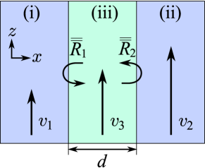
Figure 1: (Color online) A layer of moving magnetodielectric (iii) of thickness $d$ sandwiched in between two moving semiinfinite magnetodielectric layers (i) and (ii). The three layers slide along the same line which is parallel to the interfaces of the layers. The magnitudes and the signs of the velocities $v_{1,2,3}$ are arbitrary. The Casimir-Lifshitz force is calculated from the reflection matrices $\overline{\overline{R}}_{1,2}$ defined at the interfaces of the layers.

In this section we will consider the Casimir energy and force that result from the zero-point fluctuations in a layered moving medium, namely, in a configuration analogous to the canonical problem solved by Lifshitz Lifshitz (1956); Dzyaloshinski et al. (1965). Thus, we consider a structure composed of a moving layer of finite thickness $d$ sandwiched in between two other semiinfinite moving layers (Fig. 1). The velocities are assumed uniform within the layers and collinear with the $z$-axis which is parallel to the layer interfaces. Such a structure may be understood as a simplified model of a nonuniformly moving fluid, in which the width of the transition regions where the velocity changes continuously is assumed small compared to the thickness of the layers. In other words, we neglect all friction effects that may exist at the boundaries of the moving layers. In practice such situation may be achievable, for example, in certain phases of liquid helium at very low temperatures or within metamaterial layers where the velocity is merely a structural parameter (i.e., when there is no real movement).

It is evident that one may always choose a reference frame in which the middle layer is at rest. However, we prefer not to impose such a restriction, ensuring in this way a straightforward generalization of our results to the case of multiple moving layers. As follows from the treatment of Section V, in order to obtain the Casimir energy of this system, one must first solve for the reflection matrix at an interface of two moving layers. Although there are some results available in the literature (see, e.g., Huang (1994) and references therein), they are typically given in a form unsuitable for our purposes (e.g., one of the layers is assumed to be vacuum) therefore, in Appendix B we derive the necessary expressions for the components of the reflection matrices

$$\overline{\overline{R}}_{1,2}\equiv\left(\!\!\begin{array}[]{cc}R_{1,2}^{\rm ee}&R_{1,2}^{\rm eh}\\ R_{1,2}^{\rm he}&R_{1,2}^{\rm hh}\end{array}\!\!\right)$$ (54)

that are defined in terms of the $z$-components of the electric and magnetic fields. With these expressions at hand, the Casimir interaction energy in the canonical triple-layer structure is given by (53) where the matrices $\overline{\overline{R}}_{1,2}$ correspond to the two interfaces of the middle layer. From the expressions derived in Appendix B, it is also seen that the reflection matrices are invariant under a simultaneous change of signs of $\omega$ and $k_{z}$: we used this property when obtaining the expression for the zero point energy (53).

Next, the Casimir force component normal to the interfaces is found by differentiating (53) with respect to the thickness of the middle layer $d$ (we use the convention that a positive force corresponds to attraction):

$${F_{\rm c}\over L^{2}}={\hbar\over 2\pi}\int{dk_{y}\,dk_{z}\over(2\pi)^{2}}\int\limits_{0}^{\infty}{\partial\over\partial d}\log\det\left\{\overline{\overline{I^{(2)}}}-\overline{\overline{R}}_{1}\cdot\overline{\overline{R}}_{2}\,e^{-2\gamma d}\right\}d\xi=\\ ={\hbar\over 2\pi}\sum_{n=1}^{2}\int{dk_{y}\,dk_{z}\over(2\pi)^{2}}\int\limits_{0}^{\infty}{2\lambda_{n}\gamma e^{-2\gamma d}\over 1-\lambda_{n}e^{-2\gamma d}}\,d\xi,$$ (55)

where $\lambda_{1,2}$ are the eigenvalues of the matrix $\overline{\overline{R}}_{1}\cdot\overline{\overline{R}}_{2}$. It can be shown that the same expression for the Casimir force must also hold in the case of dispersive material parameters which is discussed in Appendix C.

Because the dispersion equation for the waves in (lossless and nondispersive) moving media is not symmetric with respect to the change of sign of the frequency $\omega$, it is not anymore a function of $\omega^{2}$ as in (lossless and nondispersive) reciprocal media. Due to this asymmetry the reflection matrices $\overline{\overline{R}}_{1,2}$ are in general complex at the imaginary frequencies $\omega=i\xi$ while the respective matrices in reciprocal media are always real under the same circumstances. Therefore, in general, the eigenvalues $\lambda_{1,2}$ of the matrix $\overline{\overline{R}}_{1}\cdot\overline{\overline{R}}_{2}$ are also complex. In Section VII we will, however, show that the expression for the Casimir force always results in real numbers, due to the symmetry of the integrand of  (55).

To simplify the integral (55) further we introduce new dimensionless variables $\kappa_{y}=ck_{y}/\xi$, $\kappa_{z}=ck_{z}/\xi$, $\nu=c\gamma/\xi$, and $\zeta=\xi d/c$, in which (55) becomes

$${F_{\rm c}\over L^{2}}={\hbar c\over 2\pi d^{4}}\sum_{n=1}^{2}\int{d\kappa_{y}\,d\kappa_{z}\over(2\pi)^{2}}\int\limits_{0}^{\infty}{2\nu\lambda_{n}\zeta^{3}e^{-2\nu\zeta}\over 1-\lambda_{n}e^{-2\nu\zeta}}\,d\zeta.$$ (56)

One may notice that both $\lambda_{n}$ and $\nu$ do not depend on $\zeta$ (they depend only on the relative wavenumbers $\kappa_{y}$ and $\kappa_{z}$ because the material parameters are assumed nondispersive), therefore, by substituting $\zeta=t/(2\nu)$ we obtain

$${F_{\rm c}\over L^{2}}={\hbar c\over 16\pi d^{4}}\sum_{n=1}^{2}\int{d\kappa_{y}\,d\kappa_{z}\over(2\pi)^{2}}{\lambda_{n}\over\nu^{3}}\int\limits_{0}^{\infty}{t^{3}e^{-t}\,dt\over 1-\lambda_{n}e^{-t}}={3\hbar c\over 8\pi d^{4}}\sum_{n=1}^{2}\int{d\kappa_{y}\,d\kappa_{z}\over(2\pi)^{2}}{\mbox{Li}_{4}(\lambda_{n})\over\nu^{3}},$$ (57)

where the integral over $t$ results in the polylogarithm $\mbox{Li}_{4}(z)=\sum_{n=1}^{\infty}z^{n}/n^{4}$.

Thus, the Casimir force in layers of moving (nondispersive) media has the same dependence on the distance as the Casimir force between two ideally conducting plates in vacuum. It is also seen that the value and the sign of the force (57) are determined by the the eigenvalues $\lambda_{1,2}$ of the matrix $\overline{\overline{R}}_{1}\cdot\overline{\overline{R}}_{2}$, which in turn depend on the relative velocities of the layers. In the next section we will study numerically this dependence and will demonstrate that the Casimir forces in moving media may be repulsive under certain conditions.

VII Numerical examples and discussion

In this section the expression for the Casimir force (57) is analyzed numerically. It is convenient to start from discussing some properties of the reflection coefficients (54). First of all, we would like to remind that the elements of the reflection matrix (54) are defined in terms of just a single component of the electric and magnetic field vectors (see Appendix B). Therefore, in general, their values differ significantly from the classic reflection coefficients into co- and cross-polarized TM and TE waves (the cases when (54) reduces to the classic formulas are mentioned in Appendix B). For example, the magnitudes of the cross-components $R^{\rm eh}$ and $R^{\rm he}$ in our definition may exceed unity when the characteristic impedance of the layers is different from the free-space impedance $\eta_{0}$.

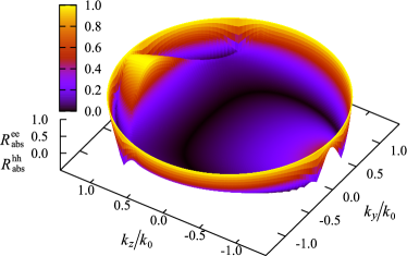
Figure 2: (Color online) The absolute values of the reflection coefficients $R_{\rm abs}^{\rm ee}=|R^{\rm ee}|$ and $R_{\rm abs}^{\rm hh}=|R^{\rm hh}|$ (the respective plots coincide and are shown with a single surface) at the real frequencies as functions of the normalized wavenumbers $k_{z}/k_{0}$ and $k_{y}/k_{0}$ at an interface of a stationary medium with $\varepsilon_{\rm r}=2$, $\mu_{\rm r}=1$ and the same medium moving with velocity $v=0.6c$. The plotted surface is colored proportionally to the reflection amplitude, as indicated in the color bar on the left.

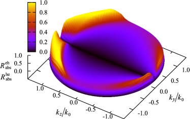
Figure 3: (Color online) The absolute values of the normalized reflection coefficients $R_{\rm abs}^{\rm eh}=|R^{\rm eh}|\sqrt{\varepsilon_{\rm r}/\mu_{\rm r}}$ and $R_{\rm abs}^{\rm he}=|R^{\rm he}|\sqrt{\mu_{\rm r}/\varepsilon_{\rm r}}$ (the plots of these functions coincide). The parameters and the rest of the legend are the same as in Fig. 2.

At real frequencies the elements of the reflection matrix (54) behave as shown in Figs. 2–3. In these figures we plot the absolute values of the reflection coefficients at an interface of a stationary medium with the relative parameters $\varepsilon_{\rm r}=2$, $\mu_{\rm r}=1$ and the same medium moving with velocity $v=0.6c$ along the $z$-axis as functions of the relative wavenumbers $k_{y}/k_{0}$ and $k_{z}/k_{0}$ (where $k_{0}=\omega/c$) of an incident wave (the wave is incident from the side of the stationary layer). The cross-components of the reflection matrix plotted in Fig. 3 are normalized as indicated in the figure caption. In these figures only the propagating waves are considered, i.e., the waves with $(k_{y}/k_{0})^{2}+(k_{z}/k_{0})^{2}\leq\varepsilon_{\rm r}\mu_{\rm r}$.

As one may notice, the elements of the reflection matrix demonstrate a strongly nonreciprocal behavior: the reflection is different for the incident waves with positive and negative $k_{z}$. It is also noticeable that the reflection is rather low overall because the parameters of the layers are chosen so that there would be no reflection if there were no movement. However, the grazing waves reflect strongly, as well as the waves with $k_{z}/k_{0}\geq(\sqrt{\varepsilon_{\rm t}\mu_{\rm t}}-a)/\sqrt{\varepsilon_{0}\mu_{0}}\approx 1.09$. The latter is due to the fact that the waves with $k_{z}$ greater than the mentioned limit are evanescent in the moving layer, as can be easily seen from the dispersion equation.

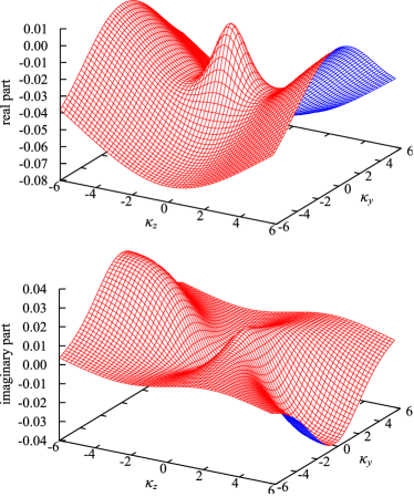
Figure 4: (Color online) Real and imaginary parts of the eigenvalues $\lambda_{1,2}$ of the matrix $\overline{\overline{R}}_{1}\cdot\overline{\overline{R}}_{2}$ at imaginary frequencies as functions of the normalized wavenumbers $\kappa_{z}$ and $\kappa_{y}$ (the plots for $\lambda_{1}$ and $\lambda_{2}$ coincide and are shown with a single surface). There are three layers of the same medium with $\varepsilon_{\rm r}=2$, $\mu_{\rm r}=1$. The middle layer is stationary and the two outer layers move with the velocity $v=0.6c$ along the positive direction of the $z$-axis.

The behavior at the imaginary frequencies is better understood from the eigenvalues $\lambda_{1,2}$ of the matrix $\overline{\overline{R}}_{1}\cdot\overline{\overline{R}}_{2}$ written for the complete structure composed of the three moving layers. Accordingly to (57), these eigenvalues determine the magnitude and the sign of the Casimir force. The plots of the eigenvalues are given in Fig. 4 for the case when the outer layers move in the same direction with velocity $v=0.6c$, and in Fig. 5 for the case when the two outer layers move with the same speed, but in the opposite directions. The middle layer is stationary in both cases.

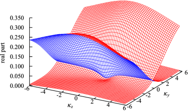
Figure 5: (Color online) The eigenvalues $\lambda_{1,2}$ at imaginary frequencies as functions of the normalized wavenumbers $\kappa_{z}$ and $\kappa_{y}$ for the case when the outer layers move in opposite directions (the eigenvalues are purely real in this scenario). The absolute value of the velocity and the other parameters are the same as in Fig. 4.

In the case when the two outer layers move in the same direction with the same velocity (Fig. 4) the two eigenvalues of the matrix $\overline{\overline{R}}_{1}\cdot\overline{\overline{R}}_{2}$ coincide. The eigenvalues are complex in this case, with the real part concentrated mostly in the negative half space, and the imaginary part changing sign when $k_{z}$ changes sign, which is a consequence of the fact that $\left(\overline{\overline{R}}_{1,2}(i\xi,k_{y},k_{z})\right)^{*}=\overline{\overline{R}}_{1,2}(-i\xi,k_{y},k_{z})=\overline{\overline{R}}_{1,2}(i\xi,k_{y},-k_{z})$ when $\xi$, $k_{y}$ and $k_{z}$ are real.

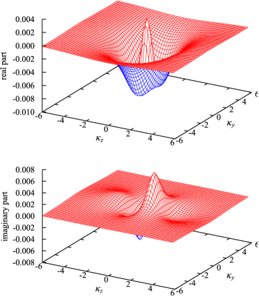
Figure 6: (Color online) The real and the imaginary parts of the integrand of Eq. (57) as functions of the normalized wavenumbers $\kappa_{z}$ and $\kappa_{y}$ in the same scenario as in Fig. 4.

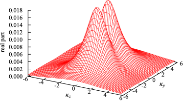
Figure 7: (Color online) The integrand of Eq. (57) as a function of the normalized wavenumbers $\kappa_{z}$ and $\kappa_{y}$ in the same scenario as in Fig. 5 (the integrand is purely real in this scenario).

When substituted into the integral (57) the dominating negative real parts of the eigenvalues result in a negative Casimir force, which corresponds to a repulsion. The contribution of the imaginary part vanishes due the symmetry of the integrand. To further illustrate this, in Fig. 6 we plot the integrand of (57) as a function of the normalized wavenumbers $\kappa_{z}$ and $\kappa_{y}$. As is seen, only a small area of the $(\kappa_{z},\kappa_{y})$ plane contributes to the integral, with the negative values of the integrand on the periphery of this area clearly outweighing the positive values seen at the middle.

When the two outer layers move in the opposite directions with the same absolute speed (Fig. 5) the eigenvalues of the matrix $\overline{\overline{R}}_{1}\cdot\overline{\overline{R}}_{2}$ are both real and positive (in a less symmetric scenario when the absolute velocities of the two layers differ there also appears a non-zero imaginary part). Thus, this case results in attraction between the two moving layers, as clearly seen from the plot of the integrand of (57) in Fig. 7. This agrees with findings of Ref. Philbin and Leonhardt (2009), where only this type of relative movement of dielectric slabs (separated by vacuum) was considered.

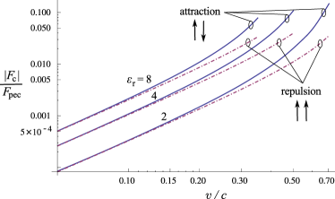
Figure 8: (Color online) The magnitude of the attractive and repulsive Casimir-Lifshitz forces in the triple-layered structures with $\mu_{\rm r}=1$ and $\varepsilon_{\rm r}$ indicated in the plot, as functions of the relative velocity $v/c$ of the outer layers (logarithmic scale). The force is normalized to the Casimir force between two perfect electric conductors (PEC) separated by the same distance as the thickness of the middle layer. The arrows in the plot indicate the directions of the movement of the outer layers that result in attraction and in repulsion.

To further study the attraction and repulsion phenomena in moving layers we have calculated the velocity dependence of the attractive and repulsive Casimir-Lifshitz forces in the two scenario considered above. The results are represented in Fig. 8. In this figure we plot the magnitude of the force $|F_{\rm c}|$ normalized to the attractive Casimir force in a system of two ideally conducting plates $F_{\rm pec}=\pi^{2}\hbar c/(240d^{4})$, where $d$ equals the thickness of the middle (stationary) layer (as we noticed in Section VI the dependence of the force on distance in layers of moving nondispersive dielectrics is the same as in Casimir’s canonical structure). Fig. 8 also demonstrates the dependence of the force on the value of the dielectric constant.

One can see that at low velocities the repulsive and attractive forces in the two scenaria of the relative movement of the outer layers are close to each other, while at larger speeds the attraction is stronger than the repulsion. The double logarithmic scale of Fig. 8 indicates that at small velocities both forces are proportional to $(v/c)^{2}$, thus, the effect reported in this paper has the same order as most of the relativistic effects. Quite naturally, the effects are more pronounced in media with higher permittivity.

In the last numerical example we calculate the attractive force between a stationary and a moving dielectric separated by a vacuum and compare it with the same force derived in Ref. Philbin and Leonhardt (2009) with an independent Green tensor-based approach. The results of this comparison can be seen in Fig. 9, where we plot $\Delta F=F(v)-F(v=0)$ which is an addition to the force that appears because of the relative movement of the layers.

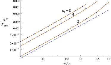
Figure 9: (Color online) The additional attractive force $\Delta F=F(v)-F(v=0)$ exerted on a dielectric with the relative permittivity $\varepsilon_{\rm r}$ moving with the relative velocity $v/c$ nearby a stationary dielectric of the same permittivity, for the three different values of the relative permittivity: 2, 4, and 8. The dielectrics are separated by a vacuum gap. The force is normalized to the Casimir force between two stationary PEC plates separated by the same gap. The brown solid lines: the force calculated with the theory of the present paper [Eq. (57)]. The blue dots: the same force calculated from Eq. (40) of Ref. Philbin and Leonhardt (2009). The blue dashed line: the plot of the $\beta^{2}$-proportional term of Eq. (42) of Ref. Philbin and Leonhardt (2009) for $\varepsilon_{\rm r}=2$.

From these calculations we conclude that up to the accuracy of numerical integration (which is a triple integration in the case of Ref. Philbin and Leonhardt (2009)) the results of the two independent approaches expressed by Eq. (57) of the present paper and Eq. (40) of Ref. Philbin and Leonhardt (2009) are in excellent agreement. The same reference contains also an expression for the leading $O(\beta^{2})$ term of the velocity-dependent correction to the Lifshitz force (Eq. (42) of Ref. Philbin and Leonhardt (2009)). However, one must be accurate when making a comparison against this result, because the (velocity-dependent) addends $A_{EE}^{-1}$ and $A_{BB}^{-1}$ seem to appear there not expanded in powers of $\beta$. A plot of the explicit $\beta^{2}$-proportional term  of the mentioned expression is shown in Fig. 9 with a blue dashed line which does not match the exact result at low velocities.

Although it is out of the scope of this paper, the observed agreement suggests that calculations of Ref. Philbin and Leonhardt (2009) are applicable to the geometries that can be considered as effectively closed ones (which is also the case of this paper) in which the pertinent difficulty with the branch cuts pointed out in Refs. Pendry (2010a, b) can be treated in a manner similar to what we have done in Appendix A. Indeed, in this work we have shown that the branch points of the reflection coefficients of moving layers are irrelevant in such geometries.

VIII Conclusions

In this paper we have considered the forces due to quantum-mechanical fluctuations of the electromagnetic field in layered moving media. We have demonstrated that rapid relative movements of neighboring layers in a dielectric (e.g., in a nonuniform fluid flow) may result in both attractive and repulsive interactions between the layers.

Although in the present study we have made an emphasis on the Casimir-Lifshitz forces resulting from relativistic movement of material layers, the results of this paper apply also (at least, qualitatively) to a class of bianisotropic metamaterials called moving media. Thus, we may conclude that a specific type of nonreciprocal magnetoelectric interaction in bianisotropic composites may also result in repulsive Casimir-Lifshitz interactions. There have been previous attempts to realize Casimir repulsion in metamaterials with the help of reciprocal magnetoelectric interaction (e.g., chirality). However, it was recently shown Silveirinha (2010); Silveirinha and Maslovski (2010a, b) that the causality and passivity preclude Casimir repulsion in reciprocal metamaterials.

The Casimir-Lifshitz interactions studied in this paper may be of importance in areas of physics involving rapid movements of matter, as well as in the phenomenological quantum electrodynamics of nonreciprocal materials.

Appendix A

The problem of branch points in the context of Casimir’s energy calculation dates back to 70’s of the last century. Some of the main ideas of the approach that we are going to use in this Appendix have been borrowed from Ref. Schram (1973).

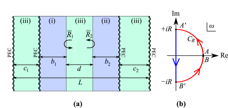
Figure 10: (Color online) (a) The PEC-backed structure used in calculation of the distant-dependent part of the zero-point energy. (b) The integration path $C$ in the complex plane of $\omega$.

Instead of considering an initially open structure, we start with the situation in which the moving layers are bounded by PEC walls, as depicted in Fig. 10(a). As is seen, there are two PEC-backed layers of media (i) and (ii) that can move in a background filled with medium (iii) that is in turn terminated by two PEC walls at $x=0$ and $x=L$. We assume that $d\ll b_{1,2}$, and $b_{1,2}\ll L$. When the PEC-backed layers (i) and (ii) move, their thicknesses $b_{1,2}$, as well as the total size of the structure $L=c_{1}+b_{1}+d+b_{2}+c_{2}$, remain fixed.

In this structure, the three regions $0<x<c_{1}$, $c_{1}<x<L-c_{2}$, and $L-c_{2}<x<L$ are electromagnetically screened from each other. Therefore, the characteristic equation for the whole structure is a product of the equations for the three regions:

$$\tilde{{\cal D}}(\gamma)=\left(1-e^{-2\gamma c_{1}}\right)^{2}\times\det\left\{\overline{\overline{I}}-\overline{\overline{R}}_{1}(\gamma)\cdot\overline{\overline{R}}_{2}(\gamma)e^{-2\gamma d}\right\}\times\left(1-e^{-2\gamma c_{2}}\right)^{2}.$$ (58)

In the middle of (58) one can recognize the term that has the form (51); we have also made explicit the dependence of terms of (58) on the propagation factor in the background medium $\gamma$.

The reflection coefficients $\overline{\overline{R}}_{1,2}$ have the following important property:

$$\overline{\overline{R}}_{1,2}(-\gamma)=\left[\overline{\overline{R}}_{1,2}(\gamma)\right]^{-1},$$ (59)

which can be seen from the fact that the reflection dyadics can be expressed as $\overline{\overline{R}}_{1,2}(\gamma)\equiv-\left[\overline{\overline{I}}+\overline{\overline{Z}}_{1,2}\cdot\overline{\overline{Y}}_{\rm w}(\gamma)\right]^{-1}\cdot\left[\overline{\overline{I}}-\overline{\overline{Z}}_{1,2}\cdot\overline{\overline{Y}}_{\rm w}(\gamma)\right]=-\left[\overline{\overline{I}}-\overline{\overline{Z}}_{1,2}\cdot\overline{\overline{Y}}_{\rm w}(\gamma)\right]\cdot\left[\overline{\overline{I}}+\overline{\overline{Z}}_{1,2}\cdot\overline{\overline{Y}}_{\rm w}(\gamma)\right]^{-1}$, where $\overline{\overline{Z}}_{1,2}$ are the dyadic input impedances of the PEC-backed layers which are meromorphic in the whole complex plane of $\omega$ and independent of $\gamma$, and $\overline{\overline{Y}}_{\rm w}(\gamma)$ is the dyadic wave admittance of the middle layer that is such that $\overline{\overline{Y}}_{\rm w}(-\gamma)=-\overline{\overline{Y}}_{\rm w}(\gamma)$. It should be noted here that while the reflection matrix of an open half space has the same property (59), the input impedance of such a space is not a meromorphic function of $\omega$ (see Ref. Schram (1973)). Thus, we may conclude that the branch points of $\overline{\overline{R}}_{1,2}$ coincide with the branch points of $\overline{\overline{Y}}_{\rm w}$ that are at the frequencies where $\gamma(\omega,k_{y},k_{z})=0$.

Using the above property we may express $\tilde{{\cal D}}(-\gamma)$ in terms of $\tilde{{\cal D}}(\gamma)$:

$$\tilde{{\cal D}}(-\gamma)=\left(1-e^{+2\gamma c_{1}}\right)^{2}\det\left\{\overline{\overline{I}}-\overline{\overline{R}}_{1}^{\,-1}\cdot\overline{\overline{R}}_{2}^{\,-1}e^{+2\gamma d}\right\}\left(1-e^{+2\gamma c_{2}}\right)^{2}={\tilde{{\cal D}}(\gamma)e^{4\gamma(L-b_{1}-b_{2})}\over\det\left\{\overline{\overline{R}}_{1}\cdot\overline{\overline{R}}_{2}\right\}},$$ (60)

where $\overline{\overline{R}}_{1,2}\equiv\overline{\overline{R}}_{1,2}(\gamma)$. From (60) one can see that the roots of function $\tilde{\cal D}(-\gamma)$ in $\omega$ include, in general, all the roots of $\tilde{\cal D}(\gamma)$. Thus, we may construct a function

$${\cal F}(\gamma)=\tilde{\cal D}(\gamma)\tilde{\cal D}(-\gamma)={\tilde{\cal D}^{2}(\gamma)\,e^{4\gamma(L-b_{1}-b_{2})}\over\det\left\{\overline{\overline{R}}_{1}\cdot\overline{\overline{R}}_{2}\right\}}={{\cal D}^{2}(\gamma)\,\left(1-e^{-2\gamma c_{1}}\right)^{4}\left(1-e^{-2\gamma c_{2}}\right)^{4}e^{4\gamma(L-b_{1}-b_{2})}\over\det\left\{\overline{\overline{R}}_{1}\cdot\overline{\overline{R}}_{2}\right\}},$$ (61)

where ${\cal D}(\gamma)\equiv\det\left\{\overline{\overline{I}}-\overline{\overline{R}}_{1}(\gamma)\cdot\overline{\overline{R}}_{2}(\gamma)e^{-2\gamma d}\right\}$ has the form (51). The function ${\cal F}(\gamma)$ has all the roots of ${\cal D}(\gamma)$ (with a difference that simple roots of ${\cal D}$ become roots of second order in ${\cal F}$) and is even in $\gamma$. The latter makes ${\cal F}(\gamma)$ a meromorphic function of $\omega$.

Therefore, we may apply the principle of argument (as explained in Section V) to this function instead of applying it directly to ${\cal D}(\gamma)$. The integral over the respective path (see Fig. 10(b)) in the complex plane of $\omega$ reads in this case

$${1\over 4\pi i}\oint\limits_{C}\omega\,d\log{\cal F}={1\over 2\pi i}\int\limits_{C_{AB}}\omega\,d\log{\cal D}+{1\over 4\pi i}\int\limits_{C_{AB}}\omega\,d\log\left[{\left(1-e^{-2\gamma c_{1}}\right)^{4}\left(1-e^{-2\gamma c_{2}}\right)^{4}}\right]+\\ +{1\over 4\pi i}\int\limits_{C_{AB}}\omega\,d\log{e^{4\gamma(L-b_{1}-b_{2})}\over\det\left\{\overline{\overline{R}}_{1}\cdot\overline{\overline{R}}_{2}\right\}},$$ (62)

where $C_{AB}$ is an open path that is obtained from $C$ by introducing a cut at the point where the semicircle crosses the real axis. Such a cut is necessary because the expressions under the integrals on the right hand side of (62) are not meromorphic in $\omega$.

Physically, the integral (62) represents a part of the zero point energy that is due to the modal frequencies which are the roots of (58) that have been encircled by the path $C$. Because we are interested only in the variation of the zero point energy with the separation $d$ between the two moving slabs, we may drop the last addend on the right hand side of (62) as it is independent of $d$. The second addend can be made arbitrary small when $c_{1,2}\rightarrow\infty$ due to the nonvanishing positive real part of $\gamma$. Thus, the distant-dependent part of the integral (62) is given by

$${1\over 2\pi i}\int\limits_{C_{AB}}\omega\,d\log{\cal D}=-{1\over 2\pi i}\int\limits_{-iR}^{+iR}\omega\,d\log{\cal D}+{1\over 2\pi i}\!\!\!\!\int\limits_{C_{AA^{\prime}}\cup C_{B^{\prime}B}}\!\!\!\!\omega\,d\log{\cal D},$$ (63)

where the first integral on the right hand side is taken over a path that lies on the imaginary axis and the second integral is over the two halves of the semicircle.

The integral (63) depends on the thicknesses of the slabs $b_{1,2}$ and the slab separation $d$. Now we let $b_{1,2}\rightarrow\infty$ in (63) (when taking this limit, we assume that still $L\gg b_{1,2}$). In this limit, due to the nonvanishing imaginary part of $\omega$ under the integrals on the right hand side of (63), the reflection coefficients of the PEC-backed layers $\overline{\overline{R}}_{1,2}$ will tend to the respective reflection coefficients of open half spaces (which are derived in Appendix B).

The last step of the derivation is to let the radius of the semicircle tend to infinity: $R\rightarrow\infty$. In this limit, which corresponds to infinitely high frequencies, all dispersive materials (including the materials with very weak dispersion that we consider in this paper) become transparent. Therefore, $\overline{\overline{R}}_{1,2}\rightarrow 0$ under the integral over the semicircle, and this integral vanishes. This leads to the expression (53) for the interaction part of the zero-point energy.

Appendix B

Let us consider an interface in a pair of layers. Without any loss of generality we let the interface be at $x=0$ with the $x$-axis orthogonal to the interface. At the interface the tangential components of the electric and magnetic fields of the two main polarizations are given by Eqs. (10)–(11):

$$\begin{split}H_{y}&=-{\omega\varepsilon_{\rm t}k_{x}\over\omega^{2}\varepsilon_{\rm t}\mu_{\rm t}-(k_{z}+\omega a)^{2}}E_{z},\\ E_{y}&=-{k_{y}(k_{z}+\omega a)\over\omega^{2}\varepsilon_{\rm t}\mu_{\rm t}-(k_{z}+\omega a)^{2}}E_{z},\\ H_{z}&=0,\end{split} (\mbox{TM}_{z})$$ (64)

$$\begin{split}E_{y}&={\omega\mu_{\rm t}k_{x}\over\omega^{2}\varepsilon_{\rm t}\mu_{\rm t}-(k_{z}+\omega a)^{2}}H_{z},\\ H_{y}&=-{k_{y}(k_{z}+\omega a)\over\omega^{2}\varepsilon_{\rm t}\mu_{\rm t}-(k_{z}+\omega a)^{2}}H_{z},\\ E_{z}&=0,\end{split} (\mbox{TE}_{z})$$ (65)

where we have replaced $k_{\rm t}^{2}$ in the denominator with an equivalent expression that follows from Eqs. (8)–(9). These relations hold at both sides of the interface, with the material parameters $\varepsilon_{\rm t}$, $\mu_{\rm t}$, and $a$, and the wave vector components taken at the respective sides.

In the following we are going to formulate and solve a plane wave reflection problem at an interface of two moving media. To simplify writing we introduce the following notations

$$\alpha =-{k_{y}(k_{z}+k_{0}a/\sqrt{\varepsilon_{0}\mu_{0}})\over k_{0}^{2}\varepsilon_{\rm t}\mu_{\rm t}/(\varepsilon_{0}\mu_{0})-(k_{z}+k_{0}a/\sqrt{\varepsilon_{0}\mu_{0}})^{2}},$$ (66)

$$\beta^{E} ={k_{0}k_{x}(\varepsilon_{\rm t}/\varepsilon_{0})\over k_{0}^{2}\varepsilon_{\rm t}\mu_{\rm t}/(\varepsilon_{0}\mu_{0})-(k_{z}+k_{0}a/\sqrt{\varepsilon_{0}\mu_{0}})^{2}},$$ (67)

$$\beta^{H} ={k_{0}k_{x}(\mu_{\rm t}/\mu_{0})\over k_{0}^{2}\varepsilon_{\rm t}\mu_{\rm t}/(\varepsilon_{0}\mu_{0})-(k_{z}+k_{0}a/\sqrt{\varepsilon_{0}\mu_{0}})^{2}},$$ (68)

where $k_{0}=\omega\sqrt{\varepsilon_{0}\mu_{0}}$. Then, with these notations at hand we consider a TM_z wave of unit amplitude incident from the region $x<0$ and write the fields in this region (the factor $e^{i(k_{y}y+k_{z}z)}$ common at both sides of the interface is dropped) as

$$E_{z} =e^{ik_{x}^{(1)}x}+Ae^{-ik_{x}^{(1)}x},$$ (69)

$$H_{z} =Be^{-ik_{x}^{(1)}x},$$ (70)

$$H_{y} =-\eta_{0}^{-1}\beta_{1}^{E}e^{ik_{x}^{(1)}x}+\eta_{0}^{-1}\beta_{1}^{E}Ae^{-ik_{x}^{(1)}x}+\alpha_{1}Be^{-ik_{x}^{(1)}x},$$ (71)

$$E_{y} =\alpha_{1}e^{ik_{x}^{(1)}x}+\alpha_{1}Ae^{-ik_{x}^{(1)}x}-\eta_{0}\beta_{1}^{H}Be^{-ik_{x}^{(1)}x},$$ (72)

and in the region $x>0$ as

$$E_{z} =Ce^{ik_{x}^{(2)}x},$$ (73)

$$H_{z} =De^{ik_{x}^{(2)}x},$$ (74)

$$H_{y} =-\eta_{0}^{-1}\beta_{2}^{E}Ce^{ik_{x}^{(2)}x}+\alpha_{2}De^{ik_{x}^{(2)}x},$$ (75)

$$E_{y} =\alpha_{2}Ce^{ik_{x}^{(2)}x}+\eta_{0}\beta_{2}^{H}De^{ik_{x}^{(2)}x},$$ (76)

where $A$, $B$, $C$, and $D$ are yet unknown wave amplitudes of the two reflected and the two transmitted waves, respectively, and $\eta_{0}=\sqrt{\mu_{0}/\varepsilon_{0}}$. As one can see, we take into account the fact that a TM_z incident wave may produce in general both polarizations in the reflected and transmitted fields.

Equating the tangential components of the electric and magnetic fields at both sides of the interface at $x\rightarrow 0$ one obtains a system of four equations for the four unknown wave amplitudes. Solving this system for $A$ and $B$ (i.e., for the reflected waves) we find

$$A =-{(\alpha_{1}-\alpha_{2})^{2}-(\beta_{1}^{E}-\beta_{2}^{E})(\beta_{1}^{H}+\beta_{2}^{H})\over(\alpha_{1}-\alpha_{2})^{2}+(\beta_{1}^{E}+\beta_{2}^{E})(\beta_{1}^{H}+\beta_{2}^{H})},$$ (77)

$$B ={2(\alpha_{1}-\alpha_{2})\beta_{1}^{E}/\eta_{0}\over(\alpha_{1}-\alpha_{2})^{2}+(\beta_{1}^{E}+\beta_{2}^{E})(\beta_{1}^{H}+\beta_{2}^{H})}.$$ (78)

The case of a TE_z incident wave can be considered in a completely analogous manner. Below we give just the final result for the amplitudes of the reflected waves:

$$A^{\prime} =-{(\alpha_{1}-\alpha_{2})^{2}-(\beta_{1}^{H}-\beta_{2}^{H})(\beta_{1}^{E}+\beta_{2}^{E})\over(\alpha_{1}-\alpha_{2})^{2}+(\beta_{1}^{H}+\beta_{2}^{H})(\beta_{1}^{E}+\beta_{2}^{E})},$$ (79)

$$B^{\prime} =-{2\eta_{0}(\alpha_{1}-\alpha_{2})\beta_{1}^{H}\over(\alpha_{1}-\alpha_{2})^{2}+(\beta_{1}^{H}+\beta_{2}^{H})(\beta_{1}^{E}+\beta_{2}^{E})}.$$ (80)

Thus, we may introduce the following reflection matrix written in terms of the $z$-components of the fields:

$$\left(\!\!\begin{array}[]{c}E_{z}^{\rm ref}\\ \eta_{0}H_{z}^{\rm ref}\end{array}\!\!\right)=\left(\!\!\begin{array}[]{cc}A&{\eta_{0}^{-1}B^{\prime}}\\ \eta_{0}B&A^{\prime}\end{array}\!\!\right)\cdot\left(\!\!\begin{array}[]{c}E_{z}^{\rm inc}\\ \eta_{0}H_{z}^{\rm inc}\end{array}\!\!\right)\equiv\left(\!\!\begin{array}[]{cc}R^{\rm ee}&R^{\rm eh}\\ R^{\rm he}&R^{\rm hh}\end{array}\!\!\right)\cdot\left(\!\!\begin{array}[]{c}E_{z}^{\rm inc}\\ \eta_{0}H_{z}^{\rm inc}\end{array}\!\!\right).$$ (81)

As can be verified, the elements of the reflection matrix reduce to the standard Fresnel reflection coefficients of the P- and S-polarized waves in the special case of $a=0$, $k_{y}=0$, for which $R^{\rm eh}=R^{\rm he}=0$, $R^{\rm ee}=R_{\rm p}\equiv\left(\varepsilon_{1}k_{x}^{(2)}-\varepsilon_{2}k_{x}^{(1)}\right)/\left(\varepsilon_{1}k_{x}^{(2)}+\varepsilon_{2}k_{x}^{(1)}\right)$ and $R^{\rm hh}=-R_{\rm s}\equiv\left(\mu_{1}k_{x}^{(2)}-\mu_{2}k_{x}^{(1)}\right)/\left(\mu_{1}k_{x}^{(2)}+\mu_{2}k_{x}^{(1)}\right)$, and also in the case of $a=0$, $k_{z}=0$, for which $R^{\rm eh}=R^{\rm he}=0$, $R^{\rm ee}=R_{\rm s}$, and $R^{\rm hh}=-R_{\rm p}$. In the general case, the standard reflection matrix defined in terms of the tangential components of the electric field can be obtained from the matrix (81) with the following similarity transformation:

$$\left(\!\!\begin{array}[]{cc}R^{yy}&R^{yz}\\ R^{zy}&R^{zz}\end{array}\!\!\right)=\left(\!\!\begin{array}[]{cc}\alpha_{1}&-\beta^{H}_{1}\\ 1&0\end{array}\!\!\right)\cdot\left(\!\!\begin{array}[]{cc}R^{\rm ee}&R^{\rm eh}\\ R^{\rm he}&R^{\rm hh}\end{array}\!\!\right)\cdot\left(\!\!\begin{array}[]{cc}\alpha_{1}&-\beta^{H}_{1}\\ 1&0\end{array}\!\!\right)^{-1}.$$ (82)

As mentioned in Section VI, the reflection coefficients (81) are in general complex, even at purely imaginary frequencies. The complexity of the reflection matrix (81) at imaginary frequencies is an unusual property that by itself deserves a separate study. Here we will only briefly outline the main reason behind this complexity. Indeed, from a physical point of view, the reflection at imaginary frequencies $\omega=i\xi$ can be understood as the response to an incident wave that has the time dependence of the form $e^{\xi t}$, i.e., to a signal that grows exponentially with time. Let us now consider an interface between a vacuum at $x<0$ and a moving medium at $x>0$, and let us assume that there is a plane wave with such time dependence impinging on the interface from the side of the the vacuum. We set up the same coordinate system as above so that the movement is along the $z$-axis. In this coordinate system the incident wave of, for instance, the TM_z polarization can be written as

$$E_{z}^{\rm inc}=E_{0}e^{i(k_{y}y+k_{z}z)}e^{\xi t-\gamma x},$$ (83)

where $k_{y}$ and $k_{z}$ are the real propagation factors in the interface plane, and $\gamma=-ik_{x}=\sqrt{\xi^{2}\varepsilon_{0}\mu_{0}+k_{y}^{2}+k_{z}^{2}}\geq 0$ is the solution of the vacuum dispersion equation at imaginary frequencies. As we are interested only in an illustration, we let $k_{y}=0$ in (83), so that the TM_z wave becomes the standard TM wave with respect to the plane of incidence.

A vacuum is invariant under the Lorentz transformations (see Section II), as are the components of the electromagnetic fields parallel to the velocity vector (the $z$-components), therefore to solve for the reflection coefficient we may switch to the comoving frame in which the reflection coefficient is simply

$$R^{\rm ee}={\varepsilon_{0}\sqrt{(\xi^{\prime})^{2}\varepsilon\mu+(k_{z}^{\prime})^{2}}-\varepsilon\sqrt{(\xi^{\prime})^{2}\varepsilon_{0}\mu_{0}+(k_{z}^{\prime})^{2}}\over\varepsilon_{0}\sqrt{(\xi^{\prime})^{2}\varepsilon\mu+(k_{z}^{\prime})^{2}}+\varepsilon\sqrt{(\xi^{\prime})^{2}\varepsilon_{0}\mu_{0}+(k_{z}^{\prime})^{2}}},$$ (84)

where

$$\xi^{\prime}={\xi+ik_{z}v\over\sqrt{1-v^{2}/c^{2}}},\quad k_{z}^{\prime}={k_{z}-i\xi v/c^{2}\over\sqrt{1-v^{2}/c^{2}}}$$ (85)

are the imaginary frequency and the $z$-component of the wave vector transformed to the comoving frame. Substituting (85) into (84) we obtain after some manipulation

$$R^{\rm ee}={\sqrt{(n^{2}-1)(\xi^{\prime}/c)^{2}+\gamma^{2}}-\varepsilon_{\rm r}\gamma\over\sqrt{(n^{2}-1)(\xi^{\prime}/c)^{2}+\gamma^{2}}+\varepsilon_{\rm r}\gamma},$$ (86)

where $\gamma=\sqrt{\xi^{2}\varepsilon_{0}\mu_{0}+k_{z}^{2}}$ and $\varepsilon_{\rm r}=\varepsilon/\varepsilon_{0}$. As is readily seen, $R^{\rm ee}$ is in general complex when $n^{2}\neq 1$ and $v\neq 0$, and this complexity is due to the fact that the relative movement of the layers intermixes the imaginary frequencies with the real-valued wavenumbers by the virtue of the Lorentz transformations. It is easy to check that the result (86) is a particular case of more general formulas (77)–(81).

Conversely, one may verify that if there exists a reference frame at which the moving matter is at rest, then under a transformation of the form (85) the complex propagation factor $\gamma(i\xi,k_{y},k_{z})$ and the reflection matrix (81) reduce to the respective expressions in stationary magnetodielectrics. Additionally, when such a transformation is applied to the integrand of (53), one may notice that the integration element $dk_{y}dk_{z}d\xi$ is preserved, because the Jacobian of the transformation (85) equals unity: $\partial(\xi,k_{z})/\partial(\xi^{\prime},k_{z}^{\prime})=1$. Therefore, the Casimir force per unity of area (the Casimir pressure) given by (53) is the same in all reference frames that move parallel to the layers, provided that the velocities of the layers are transformed accordingly to the relativistic velocity addition law. Such an invariance of the Casimir pressure (53) is not surprising, as physically the pressure exerted on the moving layers is related with the component of the photon momenta that is perpendicular to the direction of the movement, and this component is preserved under the Lorentz transformation. Thus, we may conclude that our formulation extends the known theory of Casimir-Lifshitz forces in dielectric layers in a way fully consistent with special relativity.

Appendix C

In this appendix we discuss how the results obtained for non-dispersive moving media may be generalized to include the effects of frequency dispersion in the effective material parameters.

Let us consider an isotropic dispersive magnetodielectric described by the following material relations in its proper frame:

$${\bf D}^{\prime}({\bf x}^{\prime},t^{\prime})=\varepsilon_{0}\int\limits_{0}^{\infty}{\varepsilon_{\rm r}(\tau^{\prime}){\bf E}^{\prime}({\bf x}^{\prime},t^{\prime}-\tau^{\prime})}\,d\tau^{\prime},$$ (87)

$${\bf B}^{\prime}({\bf x}^{\prime},t^{\prime})=\mu_{0}\int\limits_{0}^{\infty}{\mu_{\rm r}(\tau^{\prime}){\bf H}^{\prime}({\bf x}^{\prime},t^{\prime}-\tau^{\prime})}\,d\tau^{\prime},$$ (88)

where $\varepsilon_{\rm r}(\tau^{\prime})$ and $\mu_{\rm r}(\tau^{\prime})$ are the dielectric and magnetic response functions.

In the proper frame which is co-moving with the medium, the field components orthogonal to ${\bf v}$ can be expressed through the same components in the stationary laboratory frame as

$${\bf E}_{\rm t}^{\prime}=\gamma_{\rm L}({\bf E}_{\rm t}+{\bf v}\times{\bf B}_{\rm t}),\quad{\bf H}_{\rm t}^{\prime}=\gamma_{\rm L}({\bf H}_{\rm t}-{\bf v}\times{\bf D}_{\rm t}),$$ (89)

$${\bf D}_{\rm t}^{\prime}=\gamma_{\rm L}({\bf D}_{\rm t}+{1\over c^{2}}{\bf v}\times{\bf H}_{\rm t}),\quad{\bf B}_{\rm t}^{\prime}=\gamma_{\rm L}({\bf B}_{\rm t}-{1\over c^{2}}{\bf v}\times{\bf E}_{\rm t}),$$ (90)

where ${\bf v}$ is the medium velocity (along $Oz$) and $\gamma_{\rm L}=1/\sqrt{1-v^{2}/c^{2}}$. Substituting (89)–(90) into (87)–(88) one obtains

$${\bf D}_{\rm t}+{1\over c^{2}}{\bf v}\times{\bf H}_{\rm t}=\varepsilon_{0}\int\limits_{0}^{\infty}{\varepsilon_{\rm r}(\tau^{\prime})\left[{\bf E}_{\rm t}(z(z^{\prime},t^{\prime}),t(z^{\prime},t^{\prime}-\tau^{\prime}))+{\bf v}\times{\bf B}_{\rm t}(z(z^{\prime},t^{\prime}),t(z^{\prime},t^{\prime}-\tau^{\prime}))\right]}\,d\tau^{\prime},$$ (91)

$${\bf B}_{\rm t}-{1\over c^{2}}{\bf v}\times{\bf E}_{\rm t}=\mu_{0}\int\limits_{0}^{\infty}{\mu_{\rm r}(\tau^{\prime})\left[{\bf H}_{\rm t}(z(z^{\prime},t^{\prime}),t(z^{\prime},t^{\prime}-\tau^{\prime}))-{\bf v}\times{\bf D}_{\rm t}(z(z^{\prime},t^{\prime}),t(z^{\prime},t^{\prime}-\tau^{\prime}))\right]}\,d\tau^{\prime},$$ (92)

where $z=z(z^{\prime},t^{\prime})=\gamma_{\rm L}(z^{\prime}+vt^{\prime})$, $t=t(z^{\prime},t^{\prime})=\gamma_{\rm L}(t^{\prime}+vz^{\prime}/c^{2})$. From here,

$${\bf D}_{\rm t}+{1\over c^{2}}{\bf v}\times{\bf H}_{\rm t}=\varepsilon_{0}\int\limits_{0}^{\infty}{\varepsilon_{\rm r}(\tau^{\prime})\left[{\bf E}_{\rm t}(z-\gamma_{\rm L}v\tau^{\prime},t-\gamma_{\rm L}\tau^{\prime})+{\bf v}\times{\bf B}_{\rm t}(z-\gamma_{\rm L}v\tau^{\prime},t-\gamma_{\rm L}\tau^{\prime})\right]}\,d\tau^{\prime},$$ (93)

$${\bf B}_{\rm t}-{1\over c^{2}}{\bf v}\times{\bf E}_{\rm t}=\mu_{0}\int\limits_{0}^{\infty}{\mu_{\rm r}(\tau^{\prime})\left[{\bf H}_{\rm t}(z-\gamma_{\rm L}v\tau^{\prime},t-\gamma_{\rm L}\tau^{\prime})-{\bf v}\times{\bf D}_{\rm t}(z-\gamma_{\rm L}v\tau^{\prime},t-\gamma_{\rm L}\tau^{\prime})\right]}\,d\tau^{\prime}.$$ (94)

In order to obtain the constitutive relations in the laboratory frame, one has to solve the system of integral equations (93)–(94) to express ${\bf D}$ and ${\bf B}$ in terms of ${\bf E}$ and ${\bf H}$. It is evident that, in general, the above system may not result in a simple proportionality relation between the flux and field vectors. However, for plane waves this system is easily solvable and results in relations (1)–(5) of Section II with $\varepsilon=\varepsilon(\omega^{\prime})$, $\mu=\mu(\omega^{\prime})$, and $n=n(\omega^{\prime})$, where $\omega^{\prime}=\gamma_{\rm L}(\omega-k_{z}v)$ is the angular frequency in the proper frame of the moving medium. As this frequency depends on the wavenumber in the laboratory frame, the relations (1)–(5) with the modified parameters readily describe a spatially nonlocal medium, as was mentioned in Introduction.

One may also verify that such modification does not affect the frequency domain treatment of Section II. The equations (8)–(13) written for the plane waves in a moving nondispersive magnetodielectric hold also in the case of dispersive moving media if the parameters $\varepsilon_{\rm t}=\varepsilon_{\rm t}(\omega^{\prime})$, $\mu_{\rm t}=\mu_{\rm t}(\omega^{\prime})$, and $a=a(\omega^{\prime})$ are understood as $\omega^{\prime}$-dependent. Eq. (14) becomes a transcendental equation in the dispersive case. The important symmetry of Eqs. (8)–(13) with respect to the simultaneous change of signs of $\omega$ and ${\bf k}$ discussed in Section II is preserved in the dispersive case, because $\omega^{\prime}(\omega,{\bf k})=-\omega^{\prime}(-\omega,-{\bf k})$ and $\varepsilon(-\omega^{\prime})=\varepsilon^{*}(\omega^{\prime})$, $\mu(-\omega^{\prime})=\mu^{*}(\omega^{\prime})$. Thus, the generalization of the classical part of this study to the dispersive case is trivial.

The quantum-theoretical part of this paper is based on the expressions  (27)–(28) and (38) for the Hamiltonian of the free electromagnetic field. As has been mentioned in Section III, these expressions are physically understood as summations over the energies of all possible modes in a modal expansion of the electromagnetic field. Therefore, it is only natural that the same expressions must also hold in the case of frequency dispersive material parameters, provided that the basic relations for the energy $w$ and the momentum $p$ of a photon in a dispersive medium remain the same as in a vacuum: $w=\hbar\omega$, $p=\hbar k$, $w/p=\omega/k=v_{\rm ph}$. Hence, one must also expect the diagonalized form of the Hamiltonian (41) to be valid in the dispersive case, in which the modal frequencies $\omega({\bf k})$ are found from the transcendental equation (14) that must take into account the material dispersion.

Therefore, the expressions for the interaction part of the zero-point energy (53) and the Casimir force (55)–(56) must also hold in the dispersive case.

References

• Casimir (1948) H. B. G. Casimir, Proc. K. Ned. Akad. Wet. 51, 791 (1948).
• Lifshitz (1956) E. M. Lifshitz, Sov. Phys. JETP 2, 73 (1956).
• Philbin and Leonhardt (2009) T. G. Philbin and U. Leonhardt, New J. Phys. 11, 033035 (2009).
• Pendry (2010a) J. B. Pendry, New J. Phys. 12, 033028 (2010a).
• Leonhardt (2010) U. Leonhardt, New J. Phys. 12, 068001 (2010).
• Pendry (2010b) J. B. Pendry, New J. Phys. 12, 068002 (2010b).
• Barton (2010) G. Barton, New J. Phys. 12, 113045 (2010).
• Høye and Brevik (2010) J. S. Høye and I. Brevik, EPL 91, 60003 (2010).
• Boyer (1974) T. H. Boyer, Phys. Rev. A 9, 2078 (1974).
• Santos et al. (1999) F. C. Santos, A. Tenório, and A. C. Tort, Phys. Rev. D 60, 105022 (1999).
• Kenneth et al. (2002) O. Kenneth, I. Klich, A. Mann, and M. Revzen, Phys. Rev. Lett. 89, 033001 (2002).
• Rosa and Lambrecht (2010) L. Rosa and A. Lambrecht, Phys. Rev. D 82, 065025 (2010).
• Dzyaloshinski et al. (1965) I. E. Dzyaloshinski, E. M. Lifshitz, and L. P. Pitaevski, Adv. Phys. 10, 165 (1965).
• Munday et al. (2009) J. N. Munday, F. Capasso, and V. A. Parsegian, Nature 457, 170 (2009).
• Rahi and Zaheer (2010) S. J. Rahi and S. Zaheer, Phys. Rev. Lett. 104, 070405 (2010).
• Maslovski and Silveirinha (2011) S. I. Maslovski and M. G. Silveirinha, Phys. Rev. A (in print) (2011).
• Henkel and Joulain (2005) C. Henkel and K. Joulain, EPL 72, 929 (2005).
• Leonhardt and Philbin (2007) U. Leonhardt and T. G. Philbin, New J. Phys. 9, 254 (2007).
• Pirozhenko and Lambrecht (2008) I. G. Pirozhenko and A. Lambrecht, J. Phys. A: Math. Theor. 41, 164015 (2008).
• Rosa et al. (2008) F. S. Rosa, D. A. Dalvit, and P. W. Milonni, Phys. Rev. Lett. 100, 183602 (2008).
• Rosa (2009) F. S. S. Rosa, J. Phys.: Conf. Ser. 161, 012039 (2009).
• Yannopapas and Vitanov (2009) V. Yannopapas and N. V. Vitanov, Phys. Rev. Lett. 103, 120401 (2009).
• Zhao et al. (2009) R. Zhao, J. Zhou, T. Koschny, E. N. Economou, and C. M. Soukoulis, Phys. Rev. Lett. 103, 103602 (2009).
• Zhao et al. (2010) R. Zhao, T. Koschny, E. N. Economou, and C. M. Soukoulis, Phys. Rev. B 81, 235126 (2010).
• Silveirinha (2010) M. G. Silveirinha, Phys. Rev. B 82, 085101 (2010).
• Silveirinha and Maslovski (2010a) M. G. Silveirinha and S. I. Maslovski, Phys. Rev. A 82, 052508 (2010a).
• Silveirinha and Maslovski (2010b) M. G. Silveirinha and S. I. Maslovski, Phys. Rev. Lett. 105, 189301 (2010b).
• Kenneth and Klich (2006) O. Kenneth and I. Klich, Phys. Rev. Lett. 97, 160401 (2006).
• Rahi et al. (2010) S. J. Rahi, M. Kardar, and T. Emig, Phys. Rev. Lett. 105, 070404 (2010).
• Casimir and Polder (1948) H. B. G. Casimir and D. Polder, Phys. Rev. 73, 360 (1948).
• Kampen et al. (1968) N. V. Kampen, B. Nijboer, and K. Schram, Phys. Lett. A 26, 307 (1968).
• Jauch and Watson (1948) J. M. Jauch and K. M. Watson, Phys. Rev. 74, 950 (1948).
• Kong (1970) J. A. Kong, J. Appl. Phys. 41, 554 (1970).
• Matloob (2005) R. Matloob, Phys. Rev. A 71, 062105 (2005).
• Kamenetskii (1997) E. O. Kamenetskii, in Advances in Complex Electromagnetic Materials, NATO ASI, Series 3, High Technology (Kluwer Acad. Publishers, Dordrecht, 1997), vol. 28, pp. 359–376.
• Tretyakov et al. (1998) S. Tretyakov, A. Sihvola, A. Sochava, and C. Simovski, J. Electromag. Waves App. 12, 481 (1998).
• Tretyakov et al. (2008) S. A. Tretyakov, I. S. Nefedov, and P. Alitalo, New J. Phys. 10, 115028 (2008).
• Tretyakov and Nefedov (2009) S. A. Tretyakov and I. S. Nefedov, in Metamaterials 2009 (London, UK, 2009), pp. 114–116.
• Pauli (1958) W. Pauli, Theory of relativity (Pergamon Press Ltd., New York, 1958).
• Huang (1994) Y.-X. Huang, J. Appl. Phys. 76, 2575 (1994).
• Schram (1973) K. Schram, Phys. Lett. 43A, 282 (1973).