New Gauge Fields from Extension of Parallel Transport of Vector Spaces to Underlying Scalar Fields

Abstract

Gauge theories can be described by assigning a vector space $\bar{V}(x)$ to each space time point $x.$ A common set of complex numbers, $\bar{C},$ is usually assumed to be the set of scalars for all the $\bar{V}_{x}$. This is expanded here to assign a separate set of scalars, $\bar{C}_{x}$, to $\bar{V}_{x}.$ The freedom of choice of bases, expressed by the action of a gauge group operator on the $\bar{V}_{x}$, is expanded here to include the freedom of choice of scale factors, $c_{y,x},$ as elements of $GL(1,C)$ that relate $\bar{C}_{y}$ to $\bar{C}_{x}.$ A gauge field representation of $c_{y,x}$ gives two gauge fields, $\vec{A}(x)$ and $i\vec{B}(x).$ Inclusion of these fields in the covariant derivatives of Lagrangians results in $\vec{A}(x)$ appearing as a gauge boson for which mass is optional and $\vec{B}(x)$ as a massless gauge boson. $\vec{B}(x)$ appears to be the photon field. The nature of $\vec{A}(x)$ is not known at present. One does know that the coupling constant of $\vec{A}(x)$ to matter fields is very small compared to the fine structure constant.

Keywords: New gauge fields, space time dependent number structures

1 Introduction

The assignment of different vector spaces to different space time points has been used as a framework to describe some physical theories. This approach and the freedom to choose bases in the different spaces [1] has resulted in the development of several different gauge theories, such as QED and QCD. They also play an important role in the standard model [2].

This approach to gauge theories is based on the use of one common complex number field, $\bar{C}$, as the set of scalars for the vector spaces at different points. All vector space operations involving scalars have scalar values in $\bar{C}.$

Here a different approach is used in which a separate complex number field, $\bar{C}_{x},$ is associated with a vector space, $\bar{V}_{x},$ at each space time point $x.$ The scalars in scalar-vector multiplication and scalar products of vectors in $\bar{H}_{x}$ take values in $\bar{C}_{x}.$ In the following, vector spaces will be limited to be Hilbert spaces.

Some consequences of this expansion of the usual setup are explored here. The presence of different scalar fields at each point makes it possible to extend the freedom of choice of basis sets in each $\bar{H}_{x}$ [1] to include freedom of choice of complex number structures $\bar{C}_{x}$ that differ from one another by scaling factors [6, 5].

A good place to begin is with a description of parallel transformations between Hilbert spaces. Here the use of unitary parallel transform operators $U_{y,x}$ to map $\bar{H}_{x}$ onto $\bar{H}_{y}$ [3, 4] is expanded to include parallel transform operators $F_{y,x}$ to map $\bar{C}_{x}$ onto $\bar{C}_{y}.$ Both these operators define what is meant by the same vector and same number value. If $\psi_{y}$ and $\psi_{x}$ are vectors in $\bar{H}_{y}$ and $\bar{H}_{x}$, then $\psi_{y}=U_{y,x}\psi_{x}$ is the same vector in $\bar{H}_{y}$ as $\psi_{x}$ is in $\bar{H}_{x}.$ $a_{y}=F_{y,x}a_{x}$ is the same number value in $\bar{C}_{y}$ as $a_{x}$ is in $\bar{C}_{x}.$

If $U_{y,x}$ and $F_{y,x}$ are to include the freedom of choice of bases and of scaling factors, then these operators must each be factored into the product of two operators. This follows from the fact that $U_{y,x}$ cannot be represented by a matrix of numbers or used of elements of a Lie algebra. Similarly $F_{y,x}$ cannot be represented by a analytic function. This is shown in detail in the next section.

The rest of the paper is devoted to exploring consequences of scaling of the complex number fields. The description will be brief as details have been given for complex (and other types of) numbers elsewhere [5]. Also this paper expands on an earlier treatment where the scaling factors were restricted to be real numbers [6].

2 Factorization of Parallel Transforms

Factoring unitary parallel transform operators in quantum theory is necessary if one uses the usual representations of unitary operators. However it is not done in practice as it leads to nothing new in the usual treatments. However, for the purposes of this work it is useful to understand the problem as factorization is needed.

Let $\bar{H}_{x}$ and $\bar{H}_{y}$ be two $n$ dimensional Hilbert spaces at space time points $x,y$, and $U_{y,x}$ a unitary operator from $\bar{H}_{x}$ onto $\bar{H}_{y}.$ As an element of the gauge group, $U_{y,x}$ is supposed to account for the freedom of basis choice [1] between $\bar{H}_{x}$ and $\bar{H}_{y}.$

A problem arises if one attempts to represent $U_{y,x}$ as a matrix of numbers or as the exponential of Lie algebra operators. If $U_{y,x}$ is so represented, then the action of $U_{y,x}$ on a vector in $\bar{H}_{x}$ is a vector in $\bar{H}_{x}.$ It is not a vector in $\bar{H}_{y}.$

This problem can be solved by representing $U_{y,x}$ as the product of two unitary operators:

$$U_{y,x}=X_{y,x}V_{y,x}.$$ (1)

$V_{y,x}:\bar{H}_{x}\rightarrow\bar{H}_{x}$ is a map from $\bar{H}_{x}$ to $\bar{H}_{y}$, and $X_{y,x}:\bar{H}_{x}\rightarrow\bar{H}_{y}$ is a map from $\bar{H}_{x}$ to $\bar{H}_{y}.$ If $\psi$ is a field with vector value, $\psi(y),$ in $\bar{H}_{y}$, then $V_{y,x}\psi(y)_{x}=X^{{\dagger}}_{y,x}\psi(y)$ is the local representation of $\psi(y)$ in $\bar{H}_{x}.$ Here $U_{y,x}$ is a parallel transformation operator from $\bar{H}_{x}$ to $\bar{H}_{y}$ that defines the notion of sameness between the two vector spaces. $\psi(y)_{x}=U^{{\dagger}}_{y,x}\psi(y)$ is the same vector in $\bar{H}_{x}$ as $\psi(y)$ is in $\bar{H}_{y}.$ Here $V_{y,x}$ can be represented by a matrix of numbers or through use of Lie algebra operators. The fact that $X_{y,x}$ cannot be so represented is now not a problem.

If one expands the freedom of basis choice to include the freedom of choice of complex numbers as scalars, then similar problems exist for the complex numbers. As was the case for vector spaces, these problems can be solved by describing a local representation of $\bar{C}_{y}$ on $\bar{C}_{x}.$ This can be done by factoring the parallel transformation operator $F_{y,x}:\bar{C}_{x}\rightarrow\bar{C}_{y}$ into two operators:

$$F_{y,x}=W^{y}_{c}W^{c}_{x}.$$ (2)

Both $W^{y}_{c}$ and $W^{c}_{x}$ are isomorphisms with $W^{c}_{x}$ a map from $\bar{C}_{x}$ onto $\bar{C}_{x}$ and $W^{y}_{c}$ a map from $\bar{C}_{x}$ onto $\bar{C}_{y}.$ If $a_{y}$ is a number in $\bar{C}_{x}$ and $a_{x}=F^{-1}_{y,x}a_{y}$ is the same number in $\bar{C}_{x}$ as $a_{y}$ is in $\bar{C}_{y},$ then $W^{c}_{x}a_{x}=(W^{y}_{c})^{-1}a_{y}$ is the representation of $a_{y}$ in $\bar{C}_{x}.$ One can extend this to the complex number fields and define the local representation of $\bar{C}_{y}$ on $\bar{C}_{x}$ by $W^{c}_{x}\bar{C}_{x}=(W^{y}_{c})^{-1}\bar{C}_{y}.$

3 Digression

Here some material is presented to help make the material in the next section easier to understand. The mathematical logical description [7, 8] of different types of mathematical systems as structures is used here. A structure consists of a base set, $1$ or more basic operations, $0$ or more basic relations, and $1$ or more constants. The structures are required to satisfy a set of axioms appropriate for the system type being considered [8].

For example, a complex number structure is given by

$$\bar{C}=\{C,+,-,\times,\div,0,1\}.$$ (3)

$C$ with an overline denotes a structure. Without an overline, it denotes a base set. The axioms that $\bar{C}$ must satisfy are those of an algebraically closed field of characteristic $0$ [9].

The material in the next section, which is the main part of this paper, is based on the discovery that it is possible to define complex number structures (and structures of any number type) that differ from one another by arbitrary complex scaling factors. For each complex number, $c,$ one can define a structure, $\bar{C}^{c},$ on $C$ in which the number value, $c,$ in $\bar{C}$ is the identity in $\bar{C}^{c}.$ This scaling of number values between $\bar{C}^{c}$ and $\bar{C}$ requires compensatory scaling of the basic operations in $\bar{C}^{c}$ in terms of those in $\bar{C}.$ The compensatory scaling must be such that $\bar{C}^{c}$ satisfies the complex number axioms if and only if $\bar{C}$ does.

A very simple example of this scaling is quite useful to help in understanding the scaling. Let $\bar{N}$ be a structure,

$$\bar{N}=\{N,+,\times,<,0,1\},$$ (4)

for the natural numbers $0,1,2,3,\cdots.$ $\bar{N}$ satisfies the axioms [10] for the natural numbers.

Consider the even numbers $0,2,4,\cdots.$ One would expect these to also be a valid model for the natural number axioms. Here $2$ plays the role of the identity. The corresponding structure can be represented by

$$\bar{N}^{2}=\{N_{2},+_{2},\times_{2},0,1_{2}\}.$$ (5)

This is a structure in which any even number, $2n,$ in $\bar{N}$ is assigned the value $n$ in $\bar{N}^{2}.$

However, the goal is to give another representation of $\bar{N}^{2}$ in terms of the basic operations and number valuations in $\bar{N}$. This means that the number value $2,$ in $\bar{N}$ must have the properties of the identity in the other representation of $\bar{N}^{2}.$ This seems impossible as $2$ is not $1.$ Yet it is possible if one realizes that the axiomatic definition of the number $1$ is that it is the multiplicative identity.

It follows that the number value $2$ can serve as the multiplicative identity, if one changes the definition of multiplication in $\bar{N}^{2}$ to reflect the scaling. The structure $\bar{N}^{2}$ can now be written as

$$\bar{N}^{2}=\{N_{2},+,\frac{\times}{2},<,0,2.\}.$$ (6)

This shows that addition in $\bar{N}^{2}$ is the same as that in $\bar{N}$, but multiplication has changed in that a factor of $2$ has been included.

The proof that, with this definition of multiplication, the number value, $2$ is the multiplicative identity in $\bar{N}^{2}$, follows from the equivalences:

$$n_{2}\times_{2}1_{2}=n_{2}\Leftrightarrow 2n\frac{\textstyle\times}{\textstyle 2}2=2n\Leftrightarrow n\times 1=n.$$

The first equation is in $\bar{N}^{2},$ Eq. 5, the second is in $\bar{N}^{2},$ Eq. 6, and the third is in $\bar{N}.$ These equivalences show that, as required, $2$ is the multiplicative identity in $\bar{N}^{2}$ if and only if $1$ is the multiplicative identity in $\bar{N}.$

These ideas are applied in the next section to complex number structures where scaling is by a complex number $c$ that depends on space and time. Representation of $\bar{C}_{y}$ on $\bar{C}_{x}$ correspond to the descriptions of both representations of $\bar{N}^{2}$ relative to that of $\bar{N}.$

4 The Representation of $\bar{C}_{y}$ on $\bar{C}_{x}$

In this work, complex number structures are associated with each space time point. For points $x,y$ the structures, $\bar{C}_{y}$ and $\bar{C}_{x}$ are given by

$$\begin{array}[]{c}\bar{C}_{y}=\{C_{y},+_{y},-_{y},\times_{y},\div_{y},^{*_{y}},0_{y},1_{y}\}\\ \bar{C}_{x}=\{C_{x},+_{x},-_{x},\times_{x},\div_{x},^{*_{x}},0_{x},1_{x}\}.\end{array}$$ (7)

Here $C_{y}$ and $C_{x}$, without over lines are the base sets of the structures, $+,-,\times,\div$ are the basic operations, and $0,1$ are constants. The complex conjugation operation, $\mbox{}^{*}$ has been added as it simplifies the development. The subscripts denote structure membership of the operations and constants. Both $\bar{C}_{x}$ and $\bar{C}_{y}$ satisfy the axioms for complex numbers [7, 8].

The structure $\bar{C}^{c}_{x}$ where

$$\bar{C}^{c}_{x}=\{C_{x},+_{c},-_{c},\times_{c},\div_{c},^{*_{c}},0_{c},1_{c}\}$$ (8)

is defined to be the local representation of $\bar{C}_{y}$ at $x.$ Here the base set, is denoted by $C_{x}$ as it is the same set as that in $\bar{C}_{x}.$ The relations between $\bar{C}_{x},\bar{C}^{c}_{x},$ and $\bar{C}_{y}$ are given by

$$\bar{C}_{y}=W^{y}_{c}\bar{C}^{c}_{x}=W^{y}_{c}W^{c}_{x}\bar{C}_{x}.$$ (9)

It remains to give the explicit description of the structure elements of $\bar{C}^{c}_{x}$ in terms of those in $\bar{C}_{x}.$ Let $y=x+\hat{\nu}dx$ be a neighbor point of $x.$ The isomorphism $W^{c}_{x}$ is given by

$$\begin{array}[]{c}W^{c}_{x}(a_{x})=ca_{x},\\ \\ W^{c}_{x}(\pm_{x})=\pm_{x},\hskip 28.45274ptW^{c}_{x}(\times_{x})=\frac{\textstyle\times_{x}}{\textstyle c},\\ \\ W^{c}_{x}(\div_{x})=c\div_{x},\hskip 28.45274ptW^{c}_{x}((a_{x})^{*_{x}})=c(a^{*_{x}}_{x}).\end{array}$$ (10)

From this one can describe $\bar{C}^{c}_{x}$ explicitly by

$$\bar{C}^{c}_{x}=\{C_{x},+_{x},-_{x},\frac{\times_{x}}{c},c\div_{x},c(-)^{*_{x}},0_{x},1_{x}\}.$$ (11)

Here $c=c_{y,x}$ is a complex number in $\bar{C}_{x}$ that is associated with the link from $x$ to $y.$ Also, the base set $C_{x}$ is the same in both $\bar{C}^{c}_{x}$ and in $\bar{C}_{x}.$

Comparison of number values in $\bar{C}^{c}_{x}$ and $\bar{C}_{x}$ shows that that they are scaled by the factor $c.$ A number value $a_{c}$ in $\bar{C}^{c}_{x}$ corresponds to the number value $ca_{x}$ in $\bar{C}_{x}.$ Here $a_{c}$ is the same number value in $\bar{C}^{c}_{x}$ as $a_{x}$ is in $\bar{C}_{x}.$

One sees from these relations that ”correspondence” is distinct from ”sameness.” The number value in $\bar{C}_{x}$ that corresponds to $a_{c}$ in $\bar{C}^{c}_{x}$ is different from the number value in $\bar{C}_{x}$ that is the same as $a_{c}$ is in $\bar{C}^{c}_{x}.$ These two concepts coincide if and only if $c=1$. This describes the usual case where the $\bar{C}_{x}$ are all the same and can be replaced by one $\bar{C}.$

Note that $a_{c}^{*_{c}}=(ca_{x})^{*_{c}}$ corresponds to $c(a_{x})^{*_{x}}.$ It does not correspond to $c^{*_{x}}a_{x}^{*_{x}}.$ This follows from the equivalences

$$\begin{array}[]{l}1_{c}^{*_{c}}=1_{c}\Leftrightarrow(c1_{x})^{*_{c}}=c1_{x}\\ \hskip 28.45274pt\Leftrightarrow c(1_{x}^{*_{x}})=c1_{x}\Leftrightarrow 1_{x}^{*_{x}}=1_{x}.\end{array}$$

Another aspect of the relation between $\bar{C}^{c}_{x}$ and $\bar{C}_{x}$ is that one must drop the usual assumption that the elements of the base set, $C_{x},$ have fixed values, independent of the structure containing the base set. Here the number values associated with the elements of $C_{x},$ with one exception, depend on the structure containing $C_{x}.$ The element of $C_{x}$ that has value $a_{c}$ in $\bar{C}^{c}_{x}$ has value $ca_{x}$ in $\bar{C}_{x}.$ This is different from the element of $\bar{C}_{x}$ that has the same value, $a_{x},$ as $a_{c}$ is in $\bar{C}^{c}_{x}.$

Figure 1 shows the relation between the valuation of elements of $C_{x}$ in $\bar{C}_{x}$ and in $\bar{C}^{c}_{x}.$ The relations outlined above are shown by the arrows and number values in the figure.

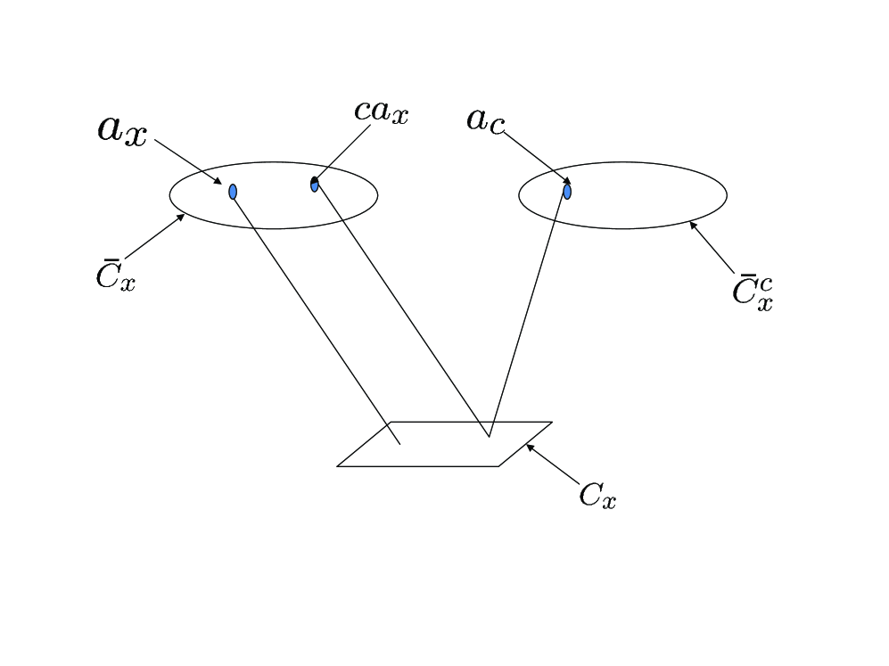
Figure 1: Relations between Elements in the base set $C_{x}$ and their Numerical Values in the Structures $\bar{C}_{x}$ and $\bar{C}^{c}_{x}.$ Here $a_{c}$ is the same number value in $\bar{C}^{c}_{x}$ as $a_{x}$ is in $\bar{C}_{x}.$ As shown by the lines they are values for different elements of $C_{x}.$ The lines also show that the $C_{x}$ element that has the value $a_{c}$ in $\bar{C}^{c}_{x}$, has the value $ca_{x}$ in $\bar{C}_{x}.$ Subscripts denote structure memberships of the number values.

The one exception is the element of $C_{x}$ that has value $0$ in $\bar{C}_{x}.$ This value is the same in all $\bar{C}^{c}_{x}$ for all values of $c.$ In this sense it is ”the number vacuum” in that it is unchanged under all transformations, $\bar{C}^{c}_{x}\rightarrow\bar{C}^{c^{\prime}}_{x}.$

The relations between the basic operations and numbers in $\bar{C}^{c}_{x}$ and those in $\bar{C}_{x}$ are not arbitrary. They are determined by the requirement that $\bar{C}_{x}$ satisfies the axioms for complex numbers [9, 11] if and only if $\bar{C}^{c}_{x}$ does. It is shown elsewhere [5, 6] that this requirement is satisfied by the relations shown in Eq. 10.

The relations between number values in $\bar{C}^{c}_{x}$ and those in $\bar{C}_{x}$ extend to terms and functions. Let $t_{c}$ be a term in $\bar{C}^{c}_{x}$ where

$$t_{c}=(\sum_{j,k=1}^{n,m})_{c}\frac{a_{c}^{j}}{b_{c}^{k}}.$$ (12)

The corresponding term in $\bar{C}_{x}$ is obtained by replacing number values, and the implied sum, multiplications, and divisions in $\bar{C}^{c}_{x}$ by their representations in $\bar{C}_{x}$ as given in Eq. 10. In this case the $j$ values and $j-1$ multiplications in the numerator give a factor of $c^{j-(j-1)}=c.$ This is canceled by a similar $c$ factor in the denominator. The solidus, as a division, contributes a factor of $c$ to give as a final result:

$$t_{c}=(\sum_{j,k=1}^{n,m})_{c}\frac{a_{c}^{j}}{b_{c}^{k}}=c(\sum_{j,k=1}^{n,m})_{x}\frac{a_{x}^{j}}{b_{x}^{k}}=ct_{x}.$$ (13)

Here $t_{x}$ is the same term in $\bar{C}_{x}$ as $t_{c}$ is in $\bar{C}^{c}_{x}.$

This result extends term by term to convergent power series and thus to analytic functions [12]. If $f_{c}(a_{c})$ is an analytic function on $\bar{C}^{c}_{x},$ then the corresponding analytic function on $\bar{C}_{x}$ is given by $cf_{x}(a_{x}).$ Here $f_{x}$ is the same function in $\bar{C}_{x}$ as $f_{c}$ is in $\bar{C}^{c}_{x}$ in that $f_{x}(a_{x})$ is the same number value in $\bar{C}_{x}$ as $f_{c}(a_{c})$ is in $\bar{C}^{c}_{x}.$

5 Gauge Fields

As was noted earlier, the above description of the local representation of $\bar{C}_{y}$ on $\bar{C}_{x},$ as in Eq. 10, is valid for $y=x+\hat{\nu}dx$ a neighbor point of $x.$ One would like to extend the description of local representations of $\bar{C}_{y}$ on $\bar{C}_{x}$ for points $y$ distant from $x.$ Also one would like to be able to use the results obtained so far in gauge theories.

These and other considerations suggest that one represent $c=c_{y,x}$ in terms of a complex valued gauge field $\vec{A}(x)+i\vec{B}(x):$

$$c_{y,x}=e^{(\vec{A}(x)+i\vec{B}(x))\cdot\hat{\nu}dx}.$$ (14)

Both $\vec{A}(x)$ and $\vec{B}(x)$ are real valued gauge fields with four space time components $A_{\mu}(x),B_{\mu}(x).$

This can be used to give an alternate expression for the action of $W^{c}_{x}$ on $\bar{C}_{x}.$ For number values one obtains from Eq. 10

$$W^{c}_{x}a_{x}=e^{(\vec{A}(x)+i\vec{B}(x))\cdot\hat{\nu}dx}a_{x}.$$ (15)

This shows that $W^{c}_{x}$ can be considered to be an element of the gauge group, $GL(1,C).$ To first order in small quantities, one has

$$\begin{array}[]{l}W^{c}_{x}(a_{x})=(1+(\vec{A}(x)+i\vec{B}(x))\cdot\hat{\nu}dx)a_{x}\\ \\ \hskip 42.67912pt=(1+(A_{\mu}(x)+iB_{\mu}(x))dx^{\mu})a_{x}.\end{array}$$ (16)

For $y$ a neighbor point of $x$, the scale change factor relating a local representation of $\bar{C}_{y}$ to $\bar{C}_{x}$ is given by

$$(\vec{A}(x)+i\vec{B}(x))\cdot\hat{\nu}dx.$$ (17)

These results can be used to define a covariant derivative of a complex number valued field, $\psi(x)$ over space time. As is well known [4], the usual derivative

$$\partial_{\mu,x}\psi=\frac{\psi(x+dx^{\mu})-\psi(x)}{dx^{\mu}}$$ (18)

is not defined as $\psi(x+dx^{\mu})$ and $\psi(x)$ are in different complex number structures. Subtraction is defined only within structures, not between structures.

This can be solved by replacing $\psi(x+dx^{\mu})$ with $\psi(x+dx^{\mu})_{x}=F^{-1}_{x+dx^{\mu},x}\psi(x+dx^{\mu})$ to obtain

$$\partial^{\prime}_{\mu,x}\psi=\frac{\psi(x+dx^{\mu})_{x}-\psi(x)}{dx^{\mu}}.$$ (19)

Here $F^{-1}_{x+dx^{\mu},x}$ is the parallel transform operator from $\bar{C}_{x+dx^{\mu}}$ to $\bar{C}_{x}$ and $\psi(x+dx^{\mu})_{x}$ is the same number value in $\bar{C}_{x}$ as $\psi(x+dx^{\mu})$ is in $\bar{C}_{x+dx^{\mu}}.$

However, this does not take into account the freedom of choice of scaling between $\bar{C}_{x+dx^{\mu}}$ and $\bar{C}_{x}.$ This extends to complex number structures, the freedom of basis choice in vector spaces that is used in gauge theories.

Taking this into account gives the covariant derivative $D_{\mu,x}$ where

$$\begin{array}[]{l}D_{\mu,x}\psi=\frac{\textstyle e^{(A_{\mu}(x)+iB_{\mu}(x))dx^{\mu}}\psi(x+dx^{\mu})_{x}-\psi(x)}{\textstyle dx^{\mu}}\\ \\ \hskip 42.67912pt=\partial^{\prime}_{\mu,x}\psi+(A_{\mu}(x)+iB_{\mu}(x))\psi(x+dx^{\mu})_{x}.\end{array}$$ (20)

The use of this in gauge theories will be discussed shortly.

5.1 Number Representation at Distant Points

So far the discussion has been pretty much limited to $y$ a neighbor point of $x.$ It needs to be extended to cases where $y$ is distant from $x.$ First consider a two step path $x\rightarrow y\rightarrow z$ where $y=x+\hat{\nu}_{1}\Delta_{x}$ and $z=y+\hat{\nu}_{2}\Delta_{y}.$ $\Delta_{y}$ and $\Delta_{x}$ are small distances with number values in $\bar{C}_{y}$ and $\bar{C}_{x}$ respectively.

Let $a_{z}$ be a number value in $\bar{C}_{z}.$ The corresponding number value in $\bar{C}_{y}$ is $c_{z,y}\times_{y}a_{y}.$ Here $c_{z,y}$ is the complex scaling factor on the link from $y$ to $z$ and $a_{y}=F^{-1}_{z,y}a_{z}$ is the same number value in $\bar{C}_{y}$ as $a_{z}$ is in $\bar{C}_{z}.$

The number value in $\bar{C}_{x}$ that corresponds to $c_{z,y}\times_{y}a_{y}$ in $\bar{C}_{y}$ is given by

$$c_{y,x}(c_{z,y})_{x}\frac{\times_{x}}{c_{y,x}}c_{y,x}a_{x}=c_{y,x}(c_{z,y})_{x}a_{x}.$$ (21)

Here $(c_{z,y})_{x}=F^{-1}_{y,x}c_{z,y}$ and $a_{x}=F^{-1}_{y,x}a_{y}$ are the same number values in $\bar{C}_{x}$ as $c_{z,y}$ and $a_{y}$ are in $\bar{C}_{y}.$

An expression equivalent to Eq.21 can be obtained by use of Eq. 16. To first order one obtains

$$\begin{array}[]{l}c_{y,x}(c_{z,y})_{x}a_{x}=[1+(\vec{A}(x)+i\vec{B}(x))\cdot\hat{\nu}_{1}\Delta_{x}+(\vec{A}(y)_{x}+i\vec{B}(y)_{x})\cdot\hat{\nu}_{2}(\Delta_{y})_{x}]a_{x}\\ \\ \hskip 56.9055pt=[1+(\vec{A}(x)+i\vec{B}(x))\cdot\hat{\nu}_{1}+(\vec{A}(y)_{x}+i\vec{B}(y)_{x})\cdot\hat{\nu}_{2}]\Delta_{x}a_{x}.\end{array}$$ (22)

Here $\vec{A}(y)_{x}$ and $\vec{B}(y)_{x}$ are the same real valued vectors at $x$ as they are at $y,$ and $(\Delta_{y})_{x}$ has been set equal to $\Delta_{x}.$

The extension to an $n$ step path is straight forward. Let $P$ be an $n$ step path where $P(0)=x_{0}=x,P(j)=x_{j},P(n-1)=x_{n-1}=y$ and $x_{j+1}=x_{j}+\hat{\nu}_{j}\Delta_{x_{j}}.$ Then

$$W^{y,P}_{x}a_{x}=c^{P}_{y,x}a_{x}$$ (23)

is the local representation of $a_{y}$ in $\bar{C}_{x}.$ Here

$$c^{P}_{y,x}=\prod_{j=0}^{n-1}(c_{x_{j+1},x_{j}})_{x}=\exp(\sum_{j=0}^{n-1}[(\vec{A}(x_{j})+i\vec{B}(x_{j}))\cdot\hat{\nu}_{j}\Delta_{x_{j}}]_{x}).$$ (24)

The subscript $x$ denotes the fact that all terms in the sum, the sum, and the exponential, are values in $\bar{C}_{x}.$ An ordering of terms in the product of Eq, 24 is not needed because the different $c$ factors commute with one another.

Let $P$ be a continuous path with points parameterized by $s$. $s$ is a continuous variable from $0$ to $1$ with $P(0)=x,P(1)=y.$ $c^{P}_{y,x}$ can be expressed in terms of the gauge fields [6] by

$$c^{P}_{y,x}=\exp\{\int_{0}^{1}(\vec{A}(P(s))_{x}+i\vec{B}(P(s))_{x})\cdot[\frac{dP(s)}{ds}]_{x}ds\}.$$ (25)

The derivative components, $[\frac{dP(s)}{ds}]_{x},$ are the same number values in $\bar{C}_{x}$ as the $\frac{dP(s)}{ds}$ are in $\bar{C}_{P(s)}.$

An equivalent expression for $c^{P}_{y,x}$ is as a line integral along the path:

$$c^{P}_{y,x}=\exp(\int_{P}(\vec{A}(z)_{x}+i\vec{B}(z)_{x})\vec{dz}).$$ (26)

The subscript $x$ indicates that the integral is defined in $\bar{C}_{x}.$

5.2 Space Integrals

The presence of the gauge fields affects space integrals of fields. As a simple example, let $\Phi(x)$ be a field where for each $x,$ $\Phi(x)$ is a number value in $\bar{C}_{x}.$ The integral, $\int\Phi(y)dy$ is supposed to be the limit of a sum $\sum_{y}\Phi(y)\Delta_{y}$ as the cubic volume elements $\Delta_{y}\rightarrow 0.$

The problem is that the sum is not defined as the elements of the sum are in different complex number structures and addition is not defined between structures. One way to fix this is to select a reference complex number structure, $\bar{C}_{x},$ and parallel transform the elements of the sum to $\bar{C}_{x}$ and then perform the summation and limit. This would give,

$$\int_{x}\Phi(y)dy=\lim_{\Delta_{x}\rightarrow 0}\sum_{y}F^{-1}_{y,x}(\Phi(y)\Delta_{y})=\lim_{\Delta_{x}\rightarrow 0}\sum_{y}\Phi(y)_{x}\Delta_{x}.$$ (27)

The subscript, $x$ on $\int$ indicates that the integral is defined on $\bar{C}_{x}.$ Also $\Phi(y)_{x}$ and $\Delta_{x}$ are the same number values in $\bar{C}_{x}$ as $\Phi(y)$ and $\Delta_{y}$ are in $\bar{C}_{y}.$

However, this representation of $\int\Phi(y)dy$ does not include the freedom of choice of scale factors. Inclusion of this freedom into the expression for the integral gives

$$\int_{x,P}\Phi(y)dy==\lim_{\Delta_{x}\rightarrow 0}\sum_{y}c^{P}_{y,x}\Phi(y)_{x}\Delta_{x}=\int c^{P}_{y,x}\Phi(y)_{x}dy_{x}.$$ (28)

Here $c^{P}_{y,x}$ is given by Eq. 24.

The problem here is the dependence of the integral on the path $P$ from $x$ to $y.$ This would introduce serious problems into the definitions of these integrals as one would have to define some sort of path integral.

This problem can be avoided if the gauge fields $\vec{A}(x)$ and $\vec{B}(x)$ are integrable. In this case $c^{P}_{y,x}$ is independent of $P$ and depends on $x$ and $y$ only. Then

$$\int c^{P}_{y,x}\Phi(y)_{x}dy_{x}=\int c_{y,x}\Phi(y)_{x}dy_{x}$$ (29)

where

$$c_{y,x}=\exp(\int(\vec{A}(z)_{x}+i\vec{B}(z)_{x})dz)$$ (30)

At present it is not known if either $\vec{A}$ or $\vec{B}$ are integrable or not. Future work should help to decide this question.

6 Other Mathematical Systems

So far the effect of choice freedom of scaling factors has been limited to complex number structures. One would expect it to also effect other mathematical systems that are based on numbers. Vector spaces are examples as they are closed under scalar vector multiplication. If they are normed spaces, then the norms are scalars.

Here Hilbert spaces are considered as examples of vector spaces. As noted in the introduction, the setup considered here consists of an assignment of a Hilbert space structure and a complex number structure, $\bar{H}_{x},\bar{C}_{x}$ to each space time point. $\bar{C}_{x}$ is the set of scalars for $\bar{H}_{x}.$

$\bar{H}_{x}$ and $\bar{H}_{y}$ are given by

$$\begin{array}[]{c}\bar{H}_{x}=\{H_{x},+_{x},-_{x},\cdot_{x},\langle-,-\rangle_{x},\psi_{x}\}\\ \bar{H}_{x}=\{H_{x},+_{x},-_{x},\cdot_{x},\langle-,-\rangle_{x},\psi_{x}\}.\end{array}$$ (31)

$H_{x}$ and $H_{y}$ denote base sets, $\cdot$ and $+,-$ denote scalar vector multiplication and linear superposition, and $\langle-,-\rangle$ denotes scalar product. The subscripts $x,y$ denote structure membership. Also $\psi_{y}$ is the same vector value in $\bar{H}_{y}$ and $\psi_{x}$ is in $\bar{H}_{x}.$ $\psi_{x},\psi_{x}$ are to be distinguished from $\psi(y)$ which is a field.

As was noted in Section 2 $\bar{H}_{y}$ and $\bar{H}_{x}$ are related by a unitary parallel transform operator $U_{y,x}$ where $\bar{H}_{y}=U_{y,x}\bar{H}_{x}.$ If $\psi_{x}$ is a vector value in $\bar{H}_{x}$, then $\psi_{y}=U_{y,x}\psi_{x}$ is the same vector value in $\bar{H}_{y}$ as $\psi_{x}$ is in $\bar{H}_{x}.$

The freedom of basis choice [1] in gauge theories [4], applied here requires the factorization of $U_{y,x}$ into two factors as in Eq. 1. This can be used to define a local representation, $\bar{H}^{V}_{x},$ of $\bar{H}_{y}$ on $\bar{H}_{x}$ by

$$\bar{H}^{V}_{x}=\{H_{x},\pm_{x}\cdot_{x},\langle-,-\rangle_{x},V_{y,x}\psi_{x}\}.$$ (32)

Here

$$V_{y,x}\psi_{x}=V_{y,x}U^{{\dagger}}_{y,x}\psi_{y}=X^{{\dagger}}_{y,x}\psi_{y}$$ (33)

is the local representation of $\psi_{y}$ at $x.$

This takes account of the freedom of basis choice but not the freedom of scaling choice for the scalar fields. This can be accounted for by defining the Hilbert space structure, $\bar{H}^{cV}_{x},$ for which $\bar{C}^{c}_{x},$ Eq. 8, is the scalar field structure. Here

$$\bar{H}^{cV}_{x}=\{H_{x},\pm^{cV}_{x},\cdot^{cV}_{x},\langle-,-\rangle^{cV}_{x},\psi^{cV}_{x}\}$$ (34)

is the local representation of $\bar{H}_{y}$ at $x.$

As was the case for complex number structures one needs to give a specific representation of the operations and vector values of $\bar{H}^{cV}_{x}$ in terms of those of $\bar{H}_{x}.$ These are given by another representation of $\bar{H}^{cV}_{x}$ as

$$\bar{H}^{cV}_{x}=\{H_{x},\pm_{x},\frac{\cdot_{x}}{c},\frac{\langle-,-\rangle_{x}}{c^{*_{x}}},cV\psi_{x}\}.$$ (35)

This representation of $\bar{H}^{cV}_{x}$ is referred to as the local representation of $\bar{H}_{y}$ on $\bar{H}_{x}.$ The scalar field for this representation is $\bar{C}^{c}_{x},$ given by Eq. 11.

It follows that the local representation, in $\bar{H}_{x},$ of a vector $\psi(y)$ in $\bar{H}_{y}$ is given by

$$X^{{\dagger}}_{y,x}\psi(y)=c_{y,x}V_{y,x}\psi(y)_{x}.$$ (36)

Here $\psi(y)_{x}=U^{-1}_{y,x}\psi(y)$ is the same vector in $\bar{H}_{x}$ as $\psi(y)$ is in $\bar{H}_{y}.$

The appearance of $c$ in the denominator of the scalar vector multiplication follows from the following equivalences:

$$\begin{array}[]{l}\phi^{cV}_{x}=a_{c}\cdot^{cV}_{x}\psi^{cV}_{x}\Leftrightarrow cV\phi_{x}=(ca_{x})\;\frac{\textstyle\cdot_{x}}{\textstyle c}\;cV\psi_{x}\\ \\ \hskip 28.45274pt\Leftrightarrow cV\phi_{x}=(ca_{x})\cdot_{x}V\psi_{x}\Leftrightarrow\phi_{x}=a_{x}\psi_{x}.\end{array}$$ (37)

These show that, as required, $\phi^{cV}_{x}=a_{c}\cdot^{cV}_{x}\psi^{cV}_{x}$ is true in $\bar{H}^{cV}_{x}$ if and only if $\phi_{x}=a_{x}\cdot_{x}\psi_{x}$ is true in $\bar{H}_{x}.$

For the scalar product in Eq. 35 the equivalences are:

$$\begin{array}[]{l}a_{c}=\langle\phi^{cV}_{x},\psi^{cV}_{x}\rangle^{cV}_{x}\Leftrightarrow ca_{x}=\langle cV\phi_{x},cV\psi_{x}\rangle_{c}\\ \\ \hskip 28.45274pt\Leftrightarrow ca_{x}=c\langle V\phi_{x},V\psi_{x}\rangle_{x}\Leftrightarrow a_{x}=\langle\phi_{x},\psi_{x}\rangle_{x}.\end{array}$$ (38)

If $|cV\phi_{x}\rangle_{c}$ in $\bar{H}^{cV}_{x}$ becomes $cV|\phi_{x}\rangle_{x}$ in $\bar{H}_{x},$ then

$$ca_{x}=\langle cV\phi_{x},cV\psi_{x}\rangle_{c}\Leftrightarrow ca_{x}=c^{*_{x}}c\frac{\textstyle\langle V\phi_{x},V\psi_{x}\rangle_{x}}{\textstyle c^{*_{x}}}\Leftrightarrow a_{x}=\langle\phi_{x},\psi_{x}\rangle_{x}.$$ (39)

Eqs. 38 and 39 show that $a_{c}=\langle\phi^{cV}_{x},\psi^{cV}_{x}\rangle^{cV}_{x}$ is true in $\bar{H}^{cV}_{x}$ and $\bar{C}^{c}_{x}$ if and only if $a_{x}=\langle\phi_{x},\psi_{x}\rangle_{x}$ is true in $\bar{H}_{x}$ and $\bar{C}_{x}.$ These equations also show the reason for $c^{*_{x}}$ as a scalar product divisor in Eq. 35

One may wonder if the presence of $c,$ as a factor multiplying $V\psi$ in Eq. 35, is needed. It is needed if one accepts the equivalence $\bar{H}\simeq\bar{C}^{n}$ [14] between $n$ dimensional Hilbert spaces and complex number tuples. Use of this for each point, $x,$ gives $\bar{H}_{y}\simeq\bar{C}^{n}_{y}.$ Similarly $\bar{H}^{cV}_{x}\simeq(\bar{C}^{c}_{x})^{n}.$ Eqs. 35 and 11 are used here.

To examine in more detail, it is sufficient to set $V=1.$ A vector in $(\bar{C}^{c}_{x})^{n}$ is a column of $n$ complex numbers, $a_{c,i}:i=1,\cdots,n.$ The corresponding column in $\bar{C}_{x}$ is $ca_{x,i}:i=1,\cdots,n.$ It follows that any vector $\psi^{c}_{x}$ in $\bar{H}^{c}_{x}$ corresponds to $c\psi_{x}$ in $\bar{H}_{x}.$

The presence of the gauge fields affects derivatives of fields. Let $\psi$ be a matter field where $\psi(x)$ is an element of $\bar{H}_{x}.$ The usual derivative

$$\partial_{\mu,x}\psi=\frac{\psi(x+dx^{\mu})-\psi(x)}{\partial x^{\mu}}$$ (40)

does not make sense because subtraction is not defined between different vector spaces.

One way to cure this is to replace $\partial_{\mu,x}$ with $\partial^{\prime}_{\mu,x}$ where

$$\partial^{\prime}_{\mu,x}\psi=\frac{\psi(x+dx^{\mu})_{x}-\psi(x)}{\partial x^{\mu}}$$ (41)

Here $\psi(x+dx^{\mu})_{x}=U^{-1}_{x+dx^{\mu},x}\psi(x+dx^{\mu})$ is the same vector in $\bar{H}_{x}$ as $\psi(x+dx^{\mu})$ is in $\bar{H}_{x+dx^{\mu}}.$

However, this does not take account of the freedom of choice of scaling introduced here or the freedom of basis choice. This is accounted for by replacing $\psi(x+dx^{\mu})_{x}$ by the local representation of $\psi(x+dx^{\mu})$ in $\bar{H}_{x}$ as given by Eq. 36. This gives the expression for the covariant derivative

$$D_{\mu,x}\psi=\frac{c_{x+dx^{\mu},x}V_{x+dx^{\mu},x}\psi(x+dx^{\mu})_{x}-\psi(x)}{\partial x^{\mu}}.$$ (42)

7 Gauge Theories

As is well known, physical Lagrangians include a covariant derivative. Examples include the Klein Gordon and Dirac Lagrangians:

$$\mathcal{L}(x)=\psi^{{\dagger}}(x)D^{\mu}_{x}D_{\mu,x}\psi-m^{2}\bar{\psi}(x)\psi(x)$$ (43)

and

$$\mathcal{L}(x)=\bar{\psi}(x)i\gamma^{\mu}D_{\mu,x}\psi-m\bar{\psi}(x)\psi(x).$$ (44)

The usual treatment uses Eq. 42 as an expression for the covariant derivative with $c_{y,x}=1$ everywhere. As such it is a special case of the setup described here.

Inclusion of the freedom of scaling choice described here results in use of Eq. 42 for the covariant derivative in Lagrangians. In this case the usual gauge group for an $n$ dimensional vector space space is expanded from $U(n)$ to $GL(1,C)\times SU(n).$ Here $c_{x+dx^{\mu},x}$ belongs to $GL(1,C)$ and $V_{x+dx^{\mu},x}$ belongs to $SU(n).$ Note that the $U(1)$ factor of $U(n)$ is not present as it is already included in $GL(1,C).$ This will be discussed more later on.

The replacement of $U(n)$ by $GL(1,C)\times SU(n)$ has consequences for both Abelian and nonabelian gauge theories. For Abelian theories the gauge group is $GL(1,C)$. For these theories, replacement of $c_{x+dx^{\mu},x}$ by its Lie algebra representation, Eq.14, and expansion to first order gives Eq. 20 which is repeated here:

$$D_{\mu,x}\psi=\partial^{\prime}_{\mu,x}\psi+(g_{R}A_{\mu}(x)+ig_{I}B_{\mu}(x))\psi(x+dx^{\mu})_{x}.$$ (45)

Coupling constants $g_{R}$ and $g_{I}$ have been added to the $\vec{A}(x)$ and $\vec{B}(x)$ fields.

One now imposes the requirement that terms in the Lagrangians are limited to those that are invariant under global and local gauge transformations [2]. For Abelian theories, global gauge transformations have the form

$$\Lambda=e^{i\phi}$$ (46)

where $\Lambda$ is a constant. Nonlocal gauge transformations have the form

$$\Lambda(x)=e^{i\phi(x)}$$ (47)

where $\Lambda(x)$ depends on $x$ through the $x$ dependence of $\phi(x).$

One replaces $\psi(x)$ in the Lagrangians with $\psi^{\prime}(x)=\Lambda(x)\psi(x)$ and examines the terms for invariance. Since $(\psi^{\prime})^{{\dagger}}(x)\psi^{\prime}(x)=\psi^{{\dagger}}\psi(x),$ terms of this form remain. For terms involving the derivative one follows the standard procedure [15]. Invariance under local gauge transformations requires that

$$D^{\prime}_{\mu,x}\Lambda\psi=\Lambda(x)D_{\mu,x}\psi$$ (48)

hold. $D^{\prime}_{\mu,x}$ is given by Eq. 45 where $A^{\prime}_{\mu}(x)$ and $B^{\prime}_{\mu}(x)$ replace $A_{\mu}(x)$ and $B_{\mu}(x).$

Solving this equation for $A^{\prime}_{\mu}(x)$ and $B^{\prime}_{\mu}(x)$ as a function of $A_{\mu}(x),B_{\mu}(x)$ and $\Lambda(x)$ gives

$$\begin{array}[]{c}A^{\prime}_{\mu}(x)=A_{\mu}(x)\\ \\ B^{\prime}_{\mu}(x)=B_{\mu}(x)+\frac{\textstyle i\Lambda^{-1}(x)\partial^{\prime}_{\mu,x}\Lambda}{\textstyle g_{I}}=B_{\mu}(x)-\frac{\textstyle\partial^{\prime}_{\mu,x}\phi(x)}{\textstyle g_{I}}\end{array}$$ (49)

These results show that $\vec{A}(x)$ is gauge invariant and that $\vec{B}(x)$ depends on the local gauge transformation. It follows from this that $\vec{A}(x)$ and $\vec{B}(x)$ correspond to two gauge bosons, $\vec{A}(x)$ can have mass in the sense that a mass term is optional in the lagrangian. However $\vec{B}(x)$ must be massless. The reason is that a mass term $\vec{B}^{{\dagger}}(x)\vec{B}(x)$ is not local gauge invariant.

The dynamics of the massless boson can be added to a Lagrangian by a Yang Mills term

$$\frac{1}{4}G_{\mu,\nu}(x)G^{\mu,\nu}(x)$$ (50)

where

$$G_{\mu,\nu}=\partial^{\prime}_{\mu,x}\vec{B}_{\nu}(x)-\partial^{\prime}_{\nu,x}B_{\mu}(x).$$ (51)

Addition of $1/4G_{\mu,\nu}G^{\mu,\nu}$ and a mass term for the $\vec{A}(x)$ field to the Dirac Lagrangian gives,

$$\begin{array}[]{l}L(x)=\bar{\psi}i\gamma^{\mu}(\partial^{\prime}_{\mu,x}+g_{R}A_{\mu}(x)+ig_{I}B_{\mu}(x))\psi-m\bar{\psi}\psi\\ \\ \hskip 28.45274pt-\frac{1}{2}\lambda^{2}A^{\mu}(x)A_{\mu}(x)-\frac{1}{4}G_{\mu,\nu}G^{\mu,\nu}.\end{array}$$ (52)

This is equivalent to the QED Lagrangian with additional terms for the $\vec{A}(x)$ field.

For nonabelian gauge theories, such as that for the gauge group $GL(1,C)\times SU(2)$ there is another equation added to Eq. 49 for the vector bosons. Since there is no change in the first two equations, the results for the vector bosons are not relevant here. A brief summary is in [6].

8 Discussion

There are some questions and problems that arise with the number scaling introduced here. The main one regards the physical nature, if any, of the $\vec{A}(x)$ and $\vec{B}(x)$ fields.

The fact that setting $\vec{A}(x)=0$ in the Dirac Lagrangian gives the QED Lagrangian suggests strongly that $\vec{B}(x)$ is the photon or electromagnetic field. In this case the coupling constant $g_{I}=e$ where $e$ is the electric charge. It is important to note that this assignment is based on the complete suppression of the $U(1)$ component of the vector space gauge group. The reason is that as far as the mathematics is concerned it contributes a gauge field that is identical to $\vec{B}(x).$ This can be seen by expanding the overall gauge group to be $GL(1,C)\times U(n)$ and carrying out the usual gauge theory treatment. If one assigns the same coupling constant to both field components, $\vec{\Gamma}(x),$ from $U(1)$ and $\vec{B}(x),$ then only the sum, $\vec{B}(x)+\vec{\Gamma}(x),$ of the fields appears in the Lagrangian. Here the $U(1)$ component is given by $\exp(i\vec{\Gamma}(x)).$

It is an open question whether the photon field is just $\vec{B}(x),\vec{\Gamma}(x),$ or a combination of both. The presence of both fields is is not likely as can be seen by considering the equivalence $\bar{H}_{x}\simeq\bar{C}^{n}_{x}.$ In this case the representation, $\bar{H}^{cV}_{x},$ Eq. 35, of $\bar{H}_{y}$ on $\bar{H}_{x}$ along with the representation, of $\bar{C}_{y}$ on $\bar{C}_{x},$ gives $\bar{H}^{cV}_{x}\simeq V_{y,x}(C^{c}_{x})^{n}.$ Here $\bar{C}^{c}_{x}$ is given by Eq. 11.

This representation argues for assigning $\vec{B}(x)$ to be the photon and $V_{y,x}$ to belong to $SU(n).$ One reason is that the Hilbert space representation is constructed from $\bar{C}^{c}_{x}$ which already has the $\vec{B}(x)$ field present. However, more work is needed here.

The physical nature of the real $\vec{A}(x)$ field is open. Candidate fields include the Higgs boson, dark matter, dark energy, and gravity. One feature that may help decide is that the coupling constant, $g_{R},$ of $\vec{A}(x)$ to matter fields must be very small compared to the fine structure constant. This is based on the great accuracy of QED.

Finally it is worth noting that the space time scaling of complex, (and other types [5] of) numbers described here may be a good approach to developing a coherent theory of physics and mathematics together [16, 17]. Clearly there is much work to do.

References

[1]
C. N. Yang and R. L. Mills, Phys. Rev. 96, 191
(1954).
[2]
S. F. Novaes, ”Particles and Fields”, Proceedings, X
Jorge Andre Swieca Summer School, Sao Paulo,
February 1999, Editors, J. Barata, M. Begalli,
R. Rosenfeld, World Scientific Publishing Co.
Singapore, 2000; Arxiv:hep-th/0001283.
[3]
G. Mack, Fortshritte der Physik, 29, 135
(1981).
[4]
I. Montvay and G. Münster, Quantum Fields on a
Lattice, Cambridge Monographs on Mathematical Physics,
Cambridge University Press, UK, 1994.
[5]
P. Benioff, arXiv 1102.3658.
[6]
P. Benioff, arXiv 1008.3134.
[7]
J. Barwise, An Introduction to First Order Logic, in
Handbook of Mathematical Logic, J. Barwise, Ed.
North-Holland Publishing Co. New York, 1977. pp 5-46.
[8]
H. J. Keisler, Fundamentals of Model Theory, in
Handbook of Mathematical Logic, J. Barwise, Ed.
North-Holland Publishing Co. New York, 1977. pp 47-104.
[9]
J. Shoenfield, Mathematical Logic, Addison Weseley
Publishing Co. Inc. Reading Ma, 1967, p. 86; Wikipedia:
Complex Numbers.
[12]
W. Rudin, Principles of Mathematical Analysis,
3rd Edition, McGraw Hill Inc. New York, 1976 Chapter 1,
”The real and complex numbers”. (Wikipedia: Real
Numbers)
[13]
R. V. Kadison and J. R, Ringrose, Fundamentals of
the Theory of Operator Algebras: Elementary theory,
Academic Press, New York, (1983), Chap 2.
[14]
R. V. Kadison and J. R, Ringrose, Fundamentals of
the Theory of Operator Algebras: Elementary theory,
Academic Press, New York, (1983), Chap 2, p. 83.
[15]
T. P. Cheng and L. F. Li, Gauge Theory of Elementary Particle Physics, Oxford University Press, Oxford, UK, (1984), Chapter 8.
[16]
P. Benioff, Found. Phys. 35, 1825-1856, (2005),
Arxiv:quant-ph/0403209.
[17]
P. Benioff, Found. Phys. 32, 989-1029, (2002),
Arxiv:quant-ph/0201093.