Statistical measures of complexity for quantum systems with continuous variables

Abstract

The Fisher-Shannon statistical measure of complexity is analyzed for a continuous manifold of quantum observables. It is shown that evaluating this measure only in the configuration or in the momentum spaces does not provide an adequate characterization of the complexity of some quantum systems. In order to obtain a more complete description of complexity two new measures, respectively based on the minimization and the integration of the usual Fisher-Shannon measure over all the parameter space, are proposed and compared. Finally, these measures are applied to the concrete case of a free particle in a box.

I Introduction

Complexity is a very interesting concept. Even if almost everyone has an intuitive conception of what complexity is an accepted mathematical definition of it is still not accepted. One reason is that this is a term that applies to very different kinds of problems, like in computer science kolmogorov:pit65 , ecology and sociology holling:01 or quantum computing mora:ijqi07 .

In recent years new mathematical measures of complexity for quantum systems with continuous variables have been proposed. The principal approach to this problem is to define a measure of complexity for a probability distribution function (pdf in brief) and then apply it to the pdf of certain variables of the system, principally the configuration ($\hat{x}$) or momentum ($\hat{p}$).

One of the most used measures of statistical complexity applied to quantum systems with continuous variables is the Fisher-Shannon measure sen_11 ; sanudo:jpa08 . The principal condition of this measure as a statistical measure of complexity is that it has its minimum value for the two extreme probability distributions, the absolutely ordered system (a Dirac delta probability distribution) and the absolutely disordered one (a highly flat distribution). These quantities have been used in the fields of non-relativistic dehesa:epjd09 ; lopezrosa:pa11 ; angulo:jcp08 ; angulo:pla08 and relativistic manzano:epl10 atomic physics and molecular chemistry lopezrosa:pccp10 , for example. Other similar measures are the LMC lopezruiz:pla95 ; anteneodo:pla96 ; catalan:pre02 and the Cramer-Rao sen:pra07 ; cover_91 , both having their minimal values for the two extreme distributions.

One important feature of these measures is their dependence on the space where they are applied. It is known that they give different results if they are calculated for the configuration or momentum pdfs and that sometimes one of these representations gives more information than the other one angulo:jcp08 , it being not trivial to realize which one will give the information for a certain state. That fact makes it necessary to check both spaces to obtaining a proper analysis of the system. Because of this reason it is complicated to say that these measures represent the complexity of the system itself but they represent the complexity of a determinate observable of the system. It is also clear that very different quantum states can give the same Fisher-Shannon measure for a concrete representation. Only in the limit where the pdf characterizes completely the state can this measure be considered an intrinsic property of the system itself.

The purpose of this paper is to analyze the dependence of the Fisher-Shannon measure when we change the basis of the system in a continuous way, and the proposal of two generalizations of it that are independent of the basis. The structure of the paper is the following: in section II the dependence of the Fisher-Shannon measure with the selected basis is analyzed, in section III we propose and justify two new measures of the complexity of a quantum system that are not calculated for an specific space, in section IV these new measures are applied to the concrete case of a particle in a box, and finally in section V some conclusions are given.

II Analysis of the basis-dependence of the Fisher-Shannon measure

It is well known that position and momentum are not the only two observables that can be defined in a quantum system. If a quantum system is defined by the state $\left|\psi\right>$ and we have a pair of one dimensional continuous observables $(\hat{x},\hat{p})$ (for simplicity we will work with one-dimensional systems, but all this reasoning can be easily extended to $D$-dimensional systems) that are canonical conjugated, the new operators defined by the unitary transformation

$$\left(\begin{array}[]{c}\hat{x}_{\theta}\\ \hat{p}_{\theta}\\ \end{array}\right)=\left(\begin{array}[]{cc}\cos\theta&-\sin\theta\\ \sin\theta&\cos\theta\\ \end{array}\right)\left(\begin{array}[]{c}\hat{x}\\ \hat{p}\\ \end{array}\right)$$ (1)

are also canonical conjugated. It is easy to check that $\hat{p}_{\theta}$ is equivalent to $\hat{x}_{\theta+\frac{\pi}{2}}$, so all the possible operators can be obtained by changing $\theta$ in the interval $\left[0,\pi\right[$. We have a continuous manifold of observables defined by the operators

$$\hat{s}_{\theta}=\cos\theta\;\hat{x}-\sin\theta\;\hat{p}\qquad\theta\in\left[0,\pi\right[.$$ (2)

where $\hat{s}_{0}$ corresponds with the position and $\hat{s}_{\frac{\pi}{2}}$ with the momentum of the system. We use the notation $\left|s_{\theta}\right>$ for the eigenvectors of the operator $\hat{s}_{\theta}$ with eigenvalue $s_{\theta}$.

For any state $\left|\psi\right>$ if we know the wavefunction for a certain parameter $s_{\theta}$ ($\left<s_{\theta}\right|\left.\psi\right>$) we can calculate the wavefunction for any other variable $s_{\theta^{\prime}}$ just by the scalar product

$$\left<s_{\theta^{\prime}}\right|\left.\psi\right>=\int_{-\infty}^{\infty}\left<s_{\theta^{\prime}}\right|\left.s_{\theta}\right>\left<s_{\theta}\right|\left.\psi\right>ds_{\theta}.$$ (3)

Finally, the probability distribution for the output of the measurement of $s_{\theta}$ can be determined in the usual way

$$\rho(s_{\theta})=\left|\left<s_{\theta}\right|\left.\psi\right>\right|^{2}$$ (4)

The Fisher-Shannon complexity in the space determined by the observable $\hat{s}_{\theta}$ is defined by the product

$$C_{FS}[\rho(s_{\theta})]:=I[\rho(s_{\theta})]\times J[\rho(s_{\theta})],$$ (5)

where

$$I[\rho(s_{\theta})] = \int_{-\infty}^{\infty}\rho(s_{\theta})\left[\frac{d}{dx}\log(\rho(s_{\theta}))\right]^{2}ds_{\theta}$$

$$J[\rho(s_{\theta})] = \frac{1}{2\pi e}\exp\left(2S[\rho(s_{\theta})]\right),$$ (6)

are the Fisher information and the entropic power of Shannon entropy, respectively. The Shannon entropy is defined as $S[\rho(s_{\theta})]:=-\int_{-\infty}^{\infty}\rho(s_{\theta})\log{\rho(s_{\theta})}ds_{\theta}$. The Fisher-Shannon measure is composed of the product of a measure of the spreading of the function, the Shannon entropic power $J[\rho]$, and a measure of possible oscillations of it, the Fisher information $I[\rho]$ cover_91 ; dehesa:epjd09 . All these quantities are based on integrating over the parameter $s_{\theta}$ and their dependence with the parameter $\theta$ is highly non-trivial.

The motivations for extending the analysis of the complexity of quantum systems to this continuous manifold of observables are two. First, as we will see, for certain systems the densities of $\hat{x}$ and $\hat{p}$ are identical, but very different to the densities of $s_{\theta}$ for a general value of $\theta$, that means that measuring this quantity only in the configuration and momentum spaces will give us a biased information. Second, in some kinds of systems, like in quantum optics, the observables defined by Eq. (1) are measurable in a simple way paul_04 so there is no reason for giving more importance to some of the observables than the others. The use of a measure defined only by the pdf of one of the observables of the system is justified if the purpose is to characterize the complexity of this concrete magnitude and not the system itself.

For testing the variation of $C_{FS}[\rho_{\theta}]$ with the parameter $\theta$ we will use the base defined by the eigenvalues of the harmonic oscillator $\left\{\left|n\right>\right\}_{n=0}^{\infty}$ ($m=\hbar=\omega=1$) in the configuration space:

$$\left<s_{0}\right|\left.n\right>=\sqrt{\frac{1}{2^{n}n!\sqrt{\pi}}}e^{-\frac{s_{0}^{2}}{2}}H_{n}(s_{0}).$$ (7)

In this case the projection (3) to the space defined by $\hat{s}_{\theta}$ gives

$$\left<s_{\theta}\right|\left.n\right>=\left<s_{0}\right|\left.n\right>e^{in\theta},$$ (8)

so the density of probability of the elements of the base does not change and the complexity is the same for any $\theta$. In Table 1 the values for the first 10 elements of the base are displayed. In a more general framework a quantum state will be a linear combination of elements of this base with norm equal to one. When more than one element are involved that situation changes dramatically and there is a highly non-trivial dependence of $C_{FS}$ with $\theta$. As an example let us take the following state

State	$C_{FS}$
$\left|1\right>$	5.15
$\left|2\right>$	11.7
$\left|3\right>$	20.5
$\left|4\right>$	31.3
$\left|5\right>$	44.2
$\left|6\right>$	59.0
$\left|7\right>$	75.7
$\left|8\right>$	94.3
$\left|9\right>$	114
$\left|10\right>$	137

Table 1: Values of the Fisher-Shannon complexity for the first ten eigenvalues of the harmonic oscillator.

$$\left|\phi_{1}(a)\right>=a\left|0\right>+\sqrt{1-a^{2}}\left|2\right>\quad a\in\mathbb{R}$$ (9)

for which the Fisher-Shannon measure gives contradictory results if it is measured only in the configuration ($\theta=0$) and momentum ($\theta=\frac{\pi}{2}$) spaces. If $a\equiv a^{+}=\frac{1}{\sqrt{2}}$ the complexities are $C_{FS}[\rho(s_{0})]=2.32$ and $C_{FS}[\rho(s_{\frac{\pi}{2}})]=2.95$; on the other hand for $a\equiv a^{-}=-\frac{1}{\sqrt{2}}$ this measure changes the roles of the configuration and momentum spaces. That transition can be easily visualized in Figure 1. By analyzing the behavior of the complexity as a function of $\theta$ we realize that the states defined by $a^{+}$ and $a^{-}$ are conjugated and they must have the same complexity.

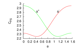
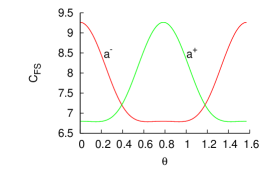
Figure 1: (Color online) Representation of the Fisher-Shannon complexity as a function of the parameter $\theta$ for the state $\left|\phi_{1}\right>$ (left) and the state $\left|\phi_{2}\right>$ (right) with $a^{\pm}=\pm\frac{1}{\sqrt{2}}$.

The reason for this contradictory results arising from the Fisher-Shannon measure in the configuration and momentum spaces is quite evident. The pdfs of position and momentum don’t give a complete description of a quantum system gale:pr68 ; only the full quantum tomogram containing all such distributions has full information on the state mancini:pla96 ; mancini:fp97 .

Observing the state

$$\left|\phi_{2}(a)\right>=a\left|0\right>+\sqrt{1-a^{2}}\left|4\right>\quad a\in\mathbb{R}.$$ (10)

For this case with $a^{+}$ we obtain $C_{FS}[\rho(s_{0})]=C_{FS}[\rho(s_{\frac{\pi}{2}})]=6.79763$ and with $a^{-}$ they are $C_{FS}[\rho(s_{0})]=C_{FS}[\rho(s_{\frac{\pi}{2}})]=9.26409$, so if we confined our analysis to only these observables we can conclude that the state $\left|\phi_{2}(a^{-})\right>$ is more complex than $\left|\phi_{2}(a^{+})\right>$. That conclusion is not truly real as can be realized by analyzing the complexity values for all the range of $\theta$. In Figure 2 it is shown that the Fisher-Shannon complexity of $\left|\phi_{2}(a^{+})\right>$ has a higher value of the complexity for a continuous interval of the parameter $\theta$, but it is impossible to realize it by calculating the complexity only in the configuration and momentum spaces. A more general measure for taking into account all the parameter space is required for that.

A usual approach to solve these kinds of problems is to use the so-called phase space, that means to work with the probability density function of $x$ and $p$. In the concrete case of $x$ and $p$ independent that is equivalent to working with the product of the complexities in both configurations angulo:jcp08 ; angulo_11 . This approach would be useful applied to the state $\left|\phi_{1}\right>$, because all the useful information can be obtain in the position or momentum spaces. On the other hand, it would give very different values for the system $\left|\phi_{2}\right>$ with $a^{+}$ and $a^{-}$, not grasping the information about all the intermediate states.

III Global and minimum Fisher-Shannon measures

One natural way for generalizing the Fisher-Shannon complexity for taking into account all the parameter space is just to integrate over all the possible values of $\theta$. That will be called the global Fisher-Shannon complexity ($C_{GFS}$), so if we have a state $\left|\psi\right>$ and $\rho(s_{\theta})=\left|\left<s_{\theta}\right|\left.\psi\right>\right|^{2}$ it is defined as

$$C_{GFS}[\left|\psi\right>]:=\frac{1}{\pi}\int_{0}^{\pi}I[\rho(s_{\theta})]\times J[\rho(s_{\theta})]d\theta,$$ (11)

where the factor $\frac{1}{\pi}$ makes this measure give the same value for the eigenvalues of the harmonic oscillator than for the usual measure.

With this new measure we can analyze again the states of Eqs (9) and (10). Now the results are independent of the sign of the parameter $a$

$$C_{GFS}\left[\left|\phi_{1}(a^{+})\right>\right]=C_{GFS}\left[\left|\phi_{1}(a^{-})\right>\right]=2.53$$

$$C_{GFS}\left[\left|\phi_{2}(a^{+})\right>\right]=C_{GFS}\left[\left|\phi_{2}(a^{-})\right>\right]=7.63$$

Now, as we are using the information about all the continuous pdfs, we can talk of the complexity of the state instead of the complexity of one determinate observable. As an example in Figure (2) the $C_{GFS}$ for the states $\left|\phi_{1}(a)\right>$ and $\left|\phi_{2}(a)\right>$ is shown for $a\in[-1,1]$. The $C_{GFS}$ has a quasilinear behavior with $a$ reaching the maximum value when $a=0$, so when the state is the eigenvalue of the harmonic oscillator with maximum complexity.

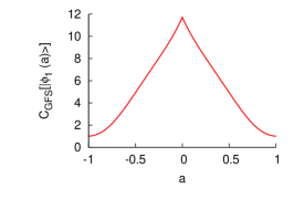
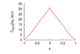
Figure 2: (Color online) Global Fisher-Shannon complexity for the state $\left|\phi_{1}(a)\right>$ (left) and $\left|\phi_{2}(a)\right>$ (right) for $a\in[-1,1]$.

It is clear that with the new measure the usual condition that is imposed for this kind of complexity measure, that it must have the minimum value for the Dirac delta and the highly flat distributions, can not be applied. That will be changed by the following condition.

Lemma: The GFS measure of complexity gives the minimum value for the states that can be represented as a gaussian distribution for any $s_{\theta}$.

Proof: If we have a quantum state $\left|\psi\right>$ for which probability density is a gaussian distribution in any space (for example for the configuration space $s_{0}$)

$$\left<s_{0}\right|\left.\psi\right>=\frac{1}{(2\pi\sigma^{2})^{\frac{1}{4}}}e^{-\frac{s_{0}^{2}}{4\sigma}},$$ (13)

the application of the projection (3) gives the wavefunction of the state $\left|\psi\right>$ for the parameter $s_{\theta}$

$$\left<s_{\theta}\right|\left.\psi\right>=\left(\frac{\sigma^{2}}{2\pi(\sin^{2}\theta+\sigma^{4}\cos^{2}\theta)}\right)^{\frac{1}{4}}e^{-\frac{s_{\theta}^{2}\sigma^{2}}{4(\sin^{2}\theta+\sigma^{4}\cos^{2}\theta)}}.$$ (14)

It is clear that if the probability of the measure of $s_{0}$ in a certain state is a gaussian distribution with $\sigma^{2}$ the distribution of measuring the quantity $s_{\theta}$ will be gaussian too with a variance $\sigma^{2}_{\theta}=\frac{\sin^{2}\theta+\sigma^{4}\cos^{2}\theta}{\sigma^{2}}$.

By direct integration of the definition (5) for a gaussian distribution we obtain that $C_{FS}=1$ independently of the variance. Due to the isoperimetric relation cover_91 $I\times J\geq 1$ (note that our pdfs come from a quantum state and they are normalized to unity in all cases), so it is clear that the Fisher-Shannon complexity has the minimum value for any gaussian distribution independently of what observable $s_{\theta}$ is represented and so the global Fisher-Shannon will be minimal for any gaussian state, because it is the integration of a function that always reaches its minimum value. This proof can be trivially extended to the $D$-dimensional problem.

The second possibility for generating a base-independent measure of complexity is to take the minimum value of the usual Fisher-Shannon in the complete range of $\theta$. That measure follows the philosophy of Kolmogorov’s complexity, that defends that the complexity of a system must be calculated in its simplest description. That will be called the minimum Fisher-Shannon measure of complexity.

$$C_{MFS}[\left|\psi\right>]:=\min_{\theta\in[0,\pi]}I[\rho(s_{\theta})]\times J[\rho(s_{\theta})].$$ (15)

This measure must be interpreted as the minimum complexity of the system for a single variable. It can happen that different states have a similar $C_{MFS}$. The interpretation of this fact is that, even if the states are different, there is some representation where they share the same complexity.

We can calculate now the minimum complexity of the states of Eqs (9) and (10). The results are similar to the global complexity.

$$C_{MFS}\left[\left|\phi_{1}(a^{+})\right>\right]=C_{MFS}\left[\left|\phi_{1}(a^{-})\right>\right]=2.25$$

$$C_{MFS}\left[\left|\phi_{2}(a^{+})\right>\right]=C_{MFS}\left[\left|\phi_{2}(a^{-})\right>\right]=6.79$$

With this definition it is possible to analyze the complexity of both states as a function of the parameter $a$ as has been plotted in Fig 2 for the GFS. The results are really very similar for both measures as can be checked in Fig. 3.

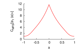
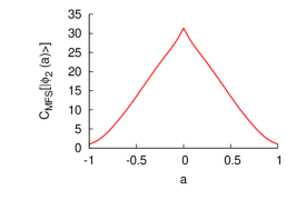
Figure 3: (Color online) Minimum Fisher-Shannon complexity for the state $\left|\phi_{1}(a)\right>$ (left) and $\left|\phi_{2}(a)\right>$ (right) for $a\in[-1,1]$.

Finally for the MFS measure we have a similar condition as we have for the GFS.

Lemma: The MFS measure of complexity gives the minimum value for the states that can be represented as a gaussian distribution for any $s_{\theta}$.

The proof is equivalent to the global case.

This new definition of complexity, as non-gaussianity, is compatible with the original Fisher-Shannon and LMC measures. These measures are usually defined by the constraint that they must be minimal for the two simplest distributions, the Dirac delta and highly flat distributions. Following the previous reasoning it is easy to check that these measures also give minimal results for any gaussian distribution, so they can be consider as measures of non-gaussianity.

These two measures are intrinsically different even if they give similar results. The global Fisher-Shannon measure gives an average measure of the complexity of describing the system in any base. That is useful if we want to take all the possibilities into account or if we have a system that cannot be easily described in an arbitrary base. The minimum Fisher-Shannon is based in Kolmogorov’s idea of complexity that states that a system is as complex as its simplest description. In both cases we are measuring how far is our system from a gaussian description. In the concrete case of being interested in a particular observable one must use the original measures, because a concrete behavior can be masked when it is mixed with all the other observables.

IV Free particle in a box

As a physical example let us see the concrete case of a one-dimensional particle in a box. This is a quantum system with a potential $V(x)=0$ if $x<a$ and an infinite potential otherwise. For simplicity we will work in a concrete system with $a=1$. The Fisher-Shannon complexity and other information-theoretical measures of this system have been recently analyzed lopezrosa:jmc11 both in position and momentum spaces.

The wavefunctions of the energy eigenstates of this system for $\theta=0$ read

$$\psi_{n}(x)=\left<s_{0}\right|\left.\psi\right>_{n}=\left\{\begin{array}[]{cc}\sin\left(\frac{\pi n}{2}(x-1)\right)&|x|\leq 1\\ 0&|x|>1\\ \end{array}\right.$$ (17)

and they can be calculated for any value of $\theta$ just by the use of relation (3). For $\theta=0$ the Fisher-Shannon measure reads lopezrosa:jmc11

$$C_{FS}[\rho_{n}(s_{0})]=\frac{8\pi n^{2}}{e^{3}}$$ (18)

and for $\theta=\frac{\pi}{2}$ it is

$$C_{FS}[\rho_{n}(s_{\frac{\pi}{2}})]=\frac{\exp(2K(n))}{24\pi e}\left(1-\frac{6}{\pi^{2}n^{2}}\right),$$ (19)

where $K(n)$ is the trigonometric integral

$$K(n) = \log\left(\frac{8}{\pi}\right)$$

$$-\pi\int_{\frac{\pi n}{2}}^{\infty}n^{2}\frac{\sin^{2}(t)}{\left(t^{2}+\pi nt\right)^{2}}\log\left[n^{2}\frac{\sin^{2}t}{\left(t^{2}+\pi nt\right)^{2}}\right]dt.$$

In Figure 4 the complexities of the first five states of this system are plotted. It is clear that these measures of complexity have a very different behavior when they are applied to one or the other base.

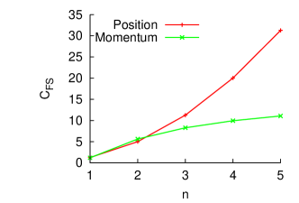
Figure 4: (Color online) Fisher-Shannon measure of complexity for a particle in a one-dimensional box in position and momentum spaces.

For understanding this behavior we must analyze the Fisher-Shannon measure for all the range of the parameter $\theta$. That measure is plotted in figure 5 (left) for the first 5 states of this system. It is clear that the behavior of the Fisher-Shannon measure as a function of the parameter $\theta$ is non-trivial, principally for small values of $\theta$. If $\theta$ approaches to $\pi/2$ the measure becomes flat and it saturates. We can analyze also the global and minimum fisher-Shannon measure for this system as a function of $n$. That is also plotted in Figure 5 (right). For this case both measures have a similar and increasing behavior. That is because the global measure is principally conditioned by the long and monotone tail that appears for $\theta>0.2$. By comparing both measures we can conclude, in general, if the complexity of the system has or not an strong variation for different descriptions. For this concrete system as both measures are very similar we can realize that the system is equally complex for a large range of $\theta$.

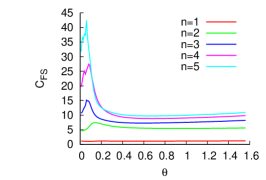
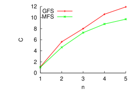
Figure 5: (Color online) Left: Fisher-Shannon measure for the first 5 energy eigenstates of a quantum particle in a box as a function of the parameter $\theta$. Right: global and minimum Fisher Shannon measures as a function of the quantum number $n$.

This example illustrate the utility of this measures. The complexity of the system close to $\theta=0$ is quite different from the rest of the parameter space. The usual Fisher-Shannon measure, the GFS and the MFS give complementary and compatible information about the system.

V Conclusions

In conclusion, we have analyzed the Fisher-Shannon measure of complexity for a continuous manifold of observables and we realize that measuring it only in the configuration and momentum spaces does not give complete information. It is clear that for certain quantum states this measure can even give contradictory results if it is not measured for all the observables. To avoid this fact we propose a global measure by the integration over all the parameter space and a second one by the minimization over it. These measures require changing the condition for statistical measures of complexity by a more general condition. These new measures will be more relevant for quantum optic systems, where all the observables involved can be measured in an experimental way. In any case, for general quantum systems, both the the global and minimum Fisher-Shannon measures must be considered more legitimate measures of the system than the usual measures because they do not depend on which spaces are calculated. Even if the definitions are made for a one-dimensional system it is trivial to extend it to the general case of a quantum system with $D$ continuous variables.

The physical example of a free particle in a box illustrates how the description of a quantum system can dramatically change if it is made for a single parameter or in general. For this concrete case the GFS and the MFS give similar results, but they are very different from the Fisher-Shannon measure in position space.

Finally, let us point out that this extension has also been applied to the LMC shape complexity lopezruiz:pla95 , and to the Cramer-Rao measure sen:pra07 giving the global LMC (GLMC), global Cramer-Rao (GCR), minimum LMC (MLMC) and minimum Cramer-Rao (MCR) measures of complexity for a quantum system. These measures have a similar behavior than the GFS and MFS. This kind of extension is also possible for other theoretically-based measures like the Jensen-Shannon divergence antolin:jcp09 .

The research was funded by the Austrian Science Fund (FWF) and the Junta de Andalucía, project FQM-165, together with the Campus de Excelencia Internacional. The author would like to acknowledge A. Lasanta and S. López-Rosa for useful discussions.

References

- (1) A. N. Kolmogorov. Three approaches to the quantitative definition of information. Probl. Inf. Transm., 1:3, 1965.
- (2) C.S. Holling. Understanding the complexity of economic, ecological, and social systems. Ecosystems, 4:390, 2001.
- (3) C. Mora, H. Briegel, and B. Kraus. Quantum kolmogorov complexity and its applications. Int. J. Quant. Inf., 5(5):729, 2007.
- (4) K.D. Sen (Editor). Statistical Complexity. Applications in Electronic Structure. Springer. Berlin, 2011.
- (5) J. Sañudo and R. López-Ruiz. Some features of the statistical complexity, Fisher-Shannon information and Bohr-like orbits in the quantum isotropic harmonic oscillator. J. Phys. A: Math. Gen., 41:265303, 2008.
- (6) J.S. Dehesa, S. López-Rosa, and D. Manzano. Configuration complexities of hydrogenic atoms. Eur. Phys. J. D., 55(3):539–548, 2009.
- (7) S. López-Rosa, D. Manzano, J.S. Dehesa Complexity of D-dimensional hydrogenic systems in position and momentum spaces Physica A: Statistical Mechanics and its Applications, 388(15):3273, 2011.
- (8) J. C. Angulo and J. Antolín. Atomic complexity measures in position and momentum spaces. J. Chem. Phys., 128:164109, 2008.
- (9) J.C. Angulo, J. Antolín, and K.D. Sen. Fisher-Shannon plane and statistical complexity of atoms. Physics Letters A, 372(5):670–674, 2008.
- (10) D. Manzano, S. López-Rosa, and J. S. Dehesa. Complexity analysis of klein-gordon single-particle systems. EPL (Europhysics Letters), 90(4):48001, 2010.
- (11) S. López-Rosa, R.O. Esquivel, J.C. Angulo, J. Antolín, J.S. Dehesa, and N. Flores-Gallegos. Analysis of complexity measures and information planes of selected molecules in position and momentum spaces. Phys. Chem. Chem. Phys., 12:7108, 2010.
- (12) R. López-Ruiz, H. L. Mancini, and X. Calbet. A statistical measure of complexity. Phys. Lett. A, 209(5-6):321–326, 1995.
- (13) R. G. Catalan, J. Garay, and R. López-Ruiz. Features of the extension of a statistical measure of complexity to continuous systems. Phys. Rev. E, 66:011102, 2002.
- (14) R. González-Férez, J.S. Dehesa, S.H. Patil, K.D. Sen Scaling properties of composite information measures and shape complexity for hydrogenic atoms in parallel magnetic and electric fields. Physica A: Statistical Mechanics and its Applications, 388(23):4919, 2009.
- (15) K. D. Sen, J. Antolín, and J. C. Angulo. Fisher-Shannon analysis of ionization processes and isoelectronic series. Phys. Rev. A, 76(3):032502, 2007.
- (16) T. M. Cover and J. A. Thomas. Elements of Information Theory. Wiley, N.Y., 1991.
- (17) H. Paul. Introduction to Quantum Optics. Cambridge University Press, 2004.
- (18) W. Gale, E. Guth, G.T. Trammell Determination of the Quantum State by MEasurements Phys. Rev. 1434:165, 1968.
- (19) S. Mancini, V.I. Manko, and P. Tombesi. Symplectic tomography as classical approach to quantum systems. Phys. Lett. A, 213:1, 1996.
- (20) S. Mancini, V.I. Manko, and P. Tombesi. Classical-like description of quantum dynamics by means of symplectic tomography. Foundations of Physics, 27:801, 1997.
- (21) J.C. Angulo, J. Antolín and R.O. Esquivel. Statistical Complexity: Applications in Electronic Structure (Chapter 6, pp. 167-213), ed. K.D. Sen (Springer, London, 2011).
- (22) S. López-Rosa, J. Montero, P. Sánchez-Moreno, J. Venegas, and J. Dehesa. Position and momentum information-theoretic measures of a 1-dimensional particle-in-a-box. Journal of Mathematical Chemistry, 49:971–994, 2011. 10.1007/s10910-010-9790-3.
- (23) J. Antolín, J.C. Angulo, and S. López-Rosa. Fisher and Jensen-Shannon divergences: quantitative comparisons among distributions. Application to position and momentum atomic densities. J. Chem. Phys., 130:074110(1–8), 2009.