Assimilating data into an $\alpha\Omega$ dynamo model
of the Sun: a variational approach

Abstract

We have developed a variational data assimilation technique for the Sun using a toy $\alpha\Omega$ dynamo model. The purpose of this work is to apply modern data assimilation techniques to solar data using a physically based model. This work represents the first step toward a complete variational model of solar magnetism. We derive the adjoint $\alpha\Omega$ dynamo code and use a minimization procedure to invert the spatial dependence of key physical ingredients of the model. We find that the variational technique is very powerful and leads to encouraging results that will be applied to a more realistic model of the solar dynamo.

1. Introduction

1.1. Predicting the solar activity

At its surface, the Sun exhibits a turbulent and very active behavior, with magnetic phenomena as diverse as sunspot emergence, flares, prominences, coronal mass ejections (CMEs). Quite unexpectedly this magnetic activity is cyclic. The full 22-year cycle is composed of two consecutive 11-year sunspot cycles (producing the so-called butterfly diagram). Coexisting with these large-scale ordered magnetic structures are small-scale but intense magnetic fluctuations that emerge over much of the solar surface, with little regard for the solar cycle (see Stix 2002, ). It is currently thought, that, in order to explain this activity and the large diversity of observed magnetic phenomena, the Sun must operate two conceptually different dynamos: a large-scale/cyclic dynamo Moffatt 1978 ; Brun et al. 2004 ; Charbonneau 2005 and a turbulent small-scale one (e.g., Cattaneo & Hughes 2001, ; Ossendrijver 2003, ).

This cyclic activity has been observed directly since the early 1600’s and traced back (indirectly) via ¹⁰Be concentration found in ice core for at least 10,000 years Beer et al. 1998 . This intense activity is known to have a direct impact on the Earth’s upper atmosphere and on our technological society. Being able to anticipate and predict the turbulent solar dynamics and magnetic activity is thus crucial if we wish to prevent damages to our satellites or interferences in our communications. This has led to the development of space weather studies and forecast. Answering key questions such as which physical processes lead to eruptive phenomena, what is the associated spectrum of solar energetic particles (SEP) and what leads to geoeffective interplanetary coronal mass ejections (ICMEs) constitute the main purpose of space weather Schwenn 2006 .

Solar eruptive phenomena are associated with active regions, i.e complexes of sunspots, that possess intricate magnetic field topology. There is a direct link between internal magnetism and these surface magnetic phenomena, since active regions are related to the emergence of strong toroidal structures most likely generated in the deep solar tachocline of intense latitudinal and radial shear at the base of the convection zone Cline 2003 ; Browning et al. 2006 ; Brun et al. 2011 . These toroidal structures become unstable, subsequently rise through the solar convection zone to appear at the surface as active regions Magara & Longcope 2003 ; Fan et al. 2003 ; Archontis et al. 2005 ; Jouve & Brun 2009 and are advected by convective motions on the solar surface (Wang & Sheeley 1991). However, the exact link between the solar cycle, CMEs and the geoeffectiveness of solar events is not straightforward to assess Pevtsov & Canfield 2001 . It is however clear that one important goal of space weather is to characterize the configurations (strength, location, field topology, etc…) that lead to geoeffective events. One way to progress in our ability to predict solar activity is to assimilate quality observations in modern numerical models of solar inner and outer magnetism (Schrijver & Derosa 2003).

Hathaway et al. (1999) summarize most of the methods used to predict the next solar cycle using historical data. Methods such as regression or curve fitting work well near solar maximum while others such as geomagnetic precursors perform better near minimum. It has also been empirically determined that odd numbered cycles are usually stronger than even numbered ones (possibly indicating a preferred orientation of the inner solar magnetic field) and that on average the cycle rises in 4.8 years and falls in 6.2 years, even though strong cycles rise faster to their maximum. A useful quantity to assess the intensity of a cycle is the yearly averaged Wolf sunspot number:

$$R=k(10g+s)$$

with $g$ the number of sunspot groups, $s$ the total number of individual sunspots in all groups and $k$ a variable scaling factor (with usually $k<1$) that accounts for instruments or observation conditions. Hathaway et al. (1999) suggest that a synthesis of current methods can provide a more accurate and useful forecast of the evolution of the Wolf number. Cycle 23 was predicted by the solar cycle 23 panel to be slightly stronger ($R\simeq 160$) than cycle 22. However with an observed value of about 120, it turned out to be almost as weak as the even numbered cycle 20 ($R=105.9$ in 1968). Further, in the prediction summary of the solar cycle 23 panel, only few of the many predictions (even by taking into account their error bars), were actually including the observed value of 120.

One thus needs to be careful with the standard indicators used up to now. The existence of a panel prediction can be seen as an attempt to use ensemble forecasting Kalnay (2003), similar to what is done in meteorology. The relative success of these methods, in particular for cycles 21 and 22 (much less so for cycle 23) could be a sign that the set of model equations used in the panel form a good ensemble. However most of the techniques considered by Hathaway et al. do not resolve the spatial dependence of the solar activity, they just focus on global properties such as number of sunspots or the timing of the next maximum. As such, these techniques are much less sophisticated than the ones used in weather forecasting. We thus need to develop more physically based forecast models of the solar cycle. Historically two types of physical models have been developed in order to understand the solar global dynamo: 2-D mean field models and 3-D magnetohydrodynamic (MHD) simulations Ossendrijver 2003 . However none of these models were used, up to very recently, to predict the evolution of the solar cycle. In order to take into account the spatial dependency of the solar activity, more recent approaches solve numerically the induction equation in a meridional plane and impose through a surface term the observed latitudinal band of activity Dikpati & Gilman 2006 ; Cameron & Schüssler 2007 ; Nandy et al. 2011 . By assimilating sunspot or meridional flow data, they try to predict the peak and timing of cycle 24.

Today, the predictions for the current solar cycle (recently summarized by the cycle 24 prediction panel) differ quite significantly from one model to another (Hathaway 2010). Some techniques, such as the ones based on geomagnetic precursors, predict a weak cycle 24 ($R<100$, Svalgaard et al. 2005, ; Duhau 2003, ; deJager & Duhau 2009, ), others based on dynamo models or meridional flow speed predict a stronger cycle ($R>140$, Dikpati et al. 2006, ; Hathaway & Wilson 2004, ). It is worth noting that all the predictions for a weak cycle 24 rely on cycle 23, i.e cycle $n$ is correlated with cycle $n-1$, whereas those predicting a strong cycle 24 (i.e stronger than cycle 23) favour a correlation with cycle 22, i.e cycle $n$ is well correlated with cycle $n-2$. The predictions of the cycle 24 panel also differ on the timing of the next maximum. In 2008, the predictions were that the maximum would occur between 2010 and 2012, depending on how fast the next cycle would rise to reach its maximum (fast if strong, slow if weak). It is now clear that the maximum will be reached late in 2013 or in 2014, confirming again the difficulty to predict the solar cycle. Some recent efforts have been undertaken to improve this situation. Kitiashvili & Kosovichev (2008) for instance have used assimilation of data in solar dynamo models to predict the solar activity (see also the work of Choudhuri et al. 2007, ; Roth 2009, ; Rempel & Dikpati 2009, ).

Assimilation of solar data in numerical models has thus already started Dikpati et al. 2004 ; Kitiashvili & Kosovichev 2008 ; Bélanger et al. 2005 ; Schrijver & DeRosa 2003 . However, intrinsic difficulties in the solar weather forecast are linked to the fact that we do not have yet a complete comprehension of the solar magnetic dynamo, cycle and surface activity. For every “piece” constituting the full puzzle, theoretical developments are still underway. This work intends to contribute to this effort.

1.2. Modern data assimilation techniques in weather forecasting

In meteorological centers, data assimilation has been operational for many decades already. Various approaches have been developed, becoming more and more sophisticated. Data assimilation can be defined as “using all available information, to determine as accurately as possible the state of the atmospheric (or oceanic) flow” Talagrand 1997 . The purpose of the work presented in this paper is to add the words ’solar flow and activity’ at the end of the quote.

Modern data assimilation techniques rely on statistical estimation theory, such as least squares methods. The generalization of such statistical methods to multivariate systems, leads to what is called the optimal interpolation (OI) for data assimilation Lorenc 1981 . Optimal interpolation consists in taking into account (assimilating) the new information that the observational data provide in order to advance in time the “background” state (also called first guess or prior information) that the weather forecasting numerical code has predicted. The increment is obtained by taking the difference, or innovation, between the observational data and the observation operator. The new state or analysis is then the result of the assimilation/forecast procedure. More specifically, let ${\bf x^{b}}$ be the background vector state characterizing the current state of the model, $H$ the observational operator and ${\bf y^{o}}$ the observational data to be assimilated in the model, then one can show that the analysis ${\bf x^{a}}$ is:

$${\bf x^{a}}={\bf x^{b}}+W({\bf y^{o}}-H({\bf x^{b}})),$$ (1)

where ${\bf y^{o}}=H({\bf x^{real}})+error$ and where $W$ represents the weights determined from the estimated statistical error covariances of the forecast and the observations Kalnay (2003). This equation is the base of modern data assimilation. The various assimilation methods will differ in the exact definition of W.

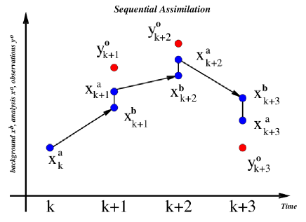
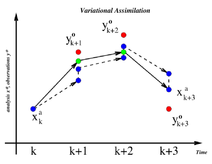
Figure 1.— Schematic representation of the sequential and 4D variational data assimilation methods used in weather forecast (adapted from Bocquet, 2011). Upper panel: in the sequential method, the background state ($x^{b}$) is updated every time observations are available (time between k and k+1) and the model evolves the state until the next step (following the arrows), at which observational data ($y^{o}$) are again assimilated to produce the analysis ($x^{a}$). Lower panel: 4D variational method and comparison with sequential assimilation. In the 4D variational method, within a time interval the model and the observations are taken into account in the cost function $\cal{J}$ that needs to be “minimized”. The minimization of this cost function results in a best trajectory (plain arrows) across the observations.

In practice, the background state, the observations and even the numerical model used to simulate the Earth’s atmosphere (i.e the primitive equations), possess errors. The assimilation methods consist in predicting the evolution of the errors and of course of minimizing it, i.e keeping it under control as much as possible given the very chaotic nature of the Earth’s atmosphere. Errors in the dynamical atmospheric system are known to double every two to three days, which leads to a predictability limit for weather forecasting that Lorenz in 1963 was the first to quantify to be of the order of 15 days. This is a very strong constraint on our ability to predict weather patterns and solar equivalent predictability limits must exist. However some atmospheric properties may be easier to predict over long periods than others, such as weekly averaged rainfall or temperature. It is likely that for the Sun, some characteristics could also be predicted over a longer period of time.

In order to have a better control of the evolution of the errors, data assimilation methods were developed and split into two categories: sequential or variational (see Talagrand 1997, ; Daley 1991, ; Kalnay, 2003). As shown in Fig.1, in the sequential methods, such as OI or Kalman filter, observational data are assimilated in the numerical model at fixed time, say every 6 hours, and then evolved forward in time. In the so called 4-D variational techniques, one seeks to minimize a cost (or misfit) function $\mbox{$\cal{J}$}({\bf\xi})$ (representing the misfit between the observations and the outputs of the model) within a certain time interval (usually 12 hours) for which data are available before making a forecast. The procedure converges when $\cal{J}$ reaches its minimum which occurs for ${\bf\xi}={\bf x^{a}}$ (see Talagrand 2003, ). Then in the next 12-hour periods, the procedure is applied again, using as background state the numerical model of the previous 12 hours. The latter technique is the one we wish to apply to the solar dynamo problem.

1.3. Variational assimilation and the adjoint method

Variational methods require the development and maintenance of a so-called adjoint model of the dynamical equations under consideration Le Dimet & Talagrand 1986 . This adjoint model computes efficiently the gradient $\partial J/\partial\xi$ necessary to the iterative minimizing procedure, by evolving backward the adjoint system of equations from the forward temporal integration Talagrand 2003 ; Kalnay (2003). Such a method is for instance also useful if one seeks to determine the gradient of a variable with respect to a large set of input variables. One can also evaluate the sensitivity of an erroneously predicted feature in the flow in order to assess which input variables are responsible for the error.

Developing an adjoint model is a straightforward but costly task and no such models have been yet developed for the full MHD system of equations (and in particular the induction equation for the magnetic field, see next sections) that is required to model the solar dynamics and magnetic activity. The development of the adjoint model of the induction equation is one purpose of this work.

Let us now enter a little bit more into the details of the adjoint procedure in order to understand how it eases the evaluation of the gradient of the cost function $\cal J$ with respect to all the input parameters (see Talagrand 1991, ).

We start by considering a composition of operations $G=G_{l}\odot G_{l-1}\odot...\odot G_{2}\odot G_{1}$ (where $G$ is a differentiable function) that, given a set of input variables $u=(u_{1},u_{2},u_{3},...,u_{n-1},u_{n})$, determines a set of output variables $v=(v_{1},v_{2},v_{3},....,v_{m-1},v_{m})$.

This process can be described by the following equation

$$v=G(u)$$ (2)

A variation $\delta v$ on the output data leads to a variation $\delta u$ of the input data that is given at first order by the tangent linear equation:

$$\delta v=G^{\prime}\delta u$$ (3)

where $G^{\prime}$ if the local Jacobian matrix of G, i.e.

$$G^{\prime}=\left(\frac{\partial v_{j}}{\partial u_{i}}\right)_{1\leq j\leq m,1\leq i\leq n}$$ (4)

Let us now consider a scalar cost function $\cal J$, function of the output variables $v$. The gradient of the function $\cal J$ with respect to the input variables $u$ reads:

$$\frac{\partial{\cal J}}{\partial u_{i}}=\sum_{j=1}^{m}\frac{\partial v_{j}}{\partial u_{i}}\frac{\partial{\cal J}}{\partial v_{j}}\,\,\,{\mbox{with}}\,\,\,i=1,...,n$$ (5)

which is in matrix notation

$$\nabla_{u}{\cal J}=G^{\prime\star}\nabla_{v}{\cal J}$$ (6)

where $G^{\prime\star}$ corresponds to the transposition of $G^{\prime}$ (hence the operator represented by the matrix $G^{\prime\star}$ is the adjoint operator of the one represented by $G^{\prime}$).

The adjoint method thus allows to compute the gradient of $\cal J$ with respect to the input variables by considering the above expression (see appendix for more details). Note that since $G$ is the composition of elementary process $(G_{k})_{k=1,...,l}$, the transpose of the Jacobian matrix $G^{\prime}$ will be the product of the transposes of the individual Jacobian matrices $G_{k}^{\prime}$, taken in the reversed order:

$$G^{\prime\star}=G_{1}^{\prime\star}\times G_{2}^{\prime\star}\times.......\times G_{l}^{\prime\star}$$ (7)

We have chosen to use this method in the framework of the solar dynamo, by applying it first to a simple $\alpha\Omega$ mean field dynamo model in Cartesian geometry. We give more details in the Appendix on how to apply it specifically to the induction equation and now describe the model used in this work.

2. The special case of the $\alpha\Omega$ dynamo

2.1. Direct $\alpha\Omega$ dynamo model

The equation we are interested in is the mean-field induction equation, derived from the standard induction equation governing the evolution of a magnetic field in the presence of a conducting fluid and dissipation, in the framework of mean-field theory. The details of the derivation of this equation can be found in Steenbeck & Raedler (1966) or Krause & Raedler (1980). The mean-field equation reads:

$$\frac{\partial{\bf B}}{\partial t}=\nabla\times({\bf v\times B})+\nabla\times(\alpha{\bf B})-\nabla\times(\eta\nabla{\bf\times B})$$ (8)

where B and v are respectively the mean magnetic and velocity fields, $\alpha$ parametrizes the physical process responsible for the regeneration of poloidal field and $\eta$ is the effective magnetic diffusivity.

We choose to work in Cartesian geometry with coordinates $(x,y,z)$, which would respectively correspond in spherical geometry to the radius, latitude and longitude. The 3 components of the magnetic field depend only on the $x$ and $y$ coordinates. The domain is defined as $[x_{1},x_{2}]\times[y_{1},y_{2}]$, with a regular grid spacing assuming $N_{x}=N_{y}=30$. For simplicity we assume that $x_{1,2}=\pm 1$ and $y_{1,2}=\pm 1$. We note that the discretization in $y$ is symmetric with respect to the equator defined by $y=0$. The poloidal/toroidal decomposition of the magnetic field then reads:

$${\bf B}(x,y,t)=\nabla\times(A(x,y,t){\bf e_{z}})+B_{z}(x,y,t){\bf e_{z}}$$ (9)

Reinjecting this poloidal/toroidal decomposition in our mean-field induction equation, we get two coupled partial differential equations, one for the poloidal potential $A$ and the other for the toroidal field $B_{z}$.

$$\frac{\partial A}{\partial t}=\alpha B_{z}+\eta(\frac{\partial^{2}A}{\partial x^{2}}+\frac{\partial^{2}A}{\partial y^{2}})$$ (10)

$$\frac{\partial B_{z}}{\partial t}=\frac{\partial v}{\partial x}\frac{\partial A}{\partial y}-\frac{\partial v}{\partial y}\frac{\partial A}{\partial x}+\eta(\frac{\partial^{2}B_{z}}{\partial x^{2}}+\frac{\partial^{2}B_{z}}{\partial y^{2}})$$ (11)

We choose to neglect the $\alpha$-effect in the equation for the toroidal field since the shear is considered to be the dominating source term. We thus consider a simple $\alpha\Omega$ dynamo model here. For boundary conditions, we assume for simplicity that both $A$ and $B_{z}$ are set to zero on the borders $x=x_{1}$ or $x_{2}$ for all $y$ and on the borders $y=y_{1}$ or $y_{2}$ for all $x$ at all times t. As initial conditions, we choose a dipolar field structure, $A$ being symmetric with respect to the equator $y=0$ and $B_{z}$ being zero everywhere.

The prescribed velocity field simply expresses as

$${\bf v}=\Omega_{0}x\sin(\pi\frac{y+1}{2}){\bf e_{z}}$$ (12)

where $\Omega_{0}$ represents the rotation rate of our domain.

We now need to give the expression for the $\alpha$-effect, responsible for the regeneration of poloidal field. We choose it to be antisymmetric with respect to the equator, as is assumed in the Sun from surface kinetic helicity measurements (Komm et al. 2007, 2008) and 3D simulations of the convective interior Miesch et al. 2000 ; Brun et al. 2004 . Its expression is the following

$$\alpha=\alpha_{0}\cos(\pi\frac{y+1}{2})$$ (13)

Finally, the magnetic diffusivity is assumed to be constant $\eta=cst$. The profile of the physical ingredients of the model are shown in Fig. 2.

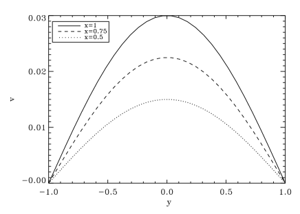
Figure 2.— Profiles of $v$ (upper panel) and $\alpha$ (lower panel) used in this simple model.

We can now nondimensionalize those equations by choosing a length scale $L$ and a temporal scale $L^{2}/\eta$. This procedure leads to the definition of physically relevant dimensionless parameters and to the new equations:

$$\frac{\partial A}{\partial t}=C_{\alpha}B_{z}+(\frac{\partial^{2}A}{\partial x^{2}}+\frac{\partial^{2}A}{\partial y^{2}})$$ (14)

$$\frac{\partial B_{z}}{\partial t}=C_{\Omega}(\frac{\partial v}{\partial x}\frac{\partial A}{\partial y}-\frac{\partial v}{\partial y}\frac{\partial A}{\partial x})+(\frac{\partial^{2}B_{z}}{\partial x^{2}}+\frac{\partial^{2}B_{z}}{\partial y^{2}})$$ (15)

with $C_{\alpha}=\alpha_{0}L/\eta$ and $C_{\Omega}=\Omega_{0}L^{2}/\eta$ the Reynolds numbers measuring the intensity of the $\alpha$ and $\Omega$ effects compared to the Ohmic dissipation. The product of those two numbers will have to be above a given threshold for dynamo action to occur.

2.2. The numerical method and choice of model parameters

Equations 14 and 15 are solved numerically using a finite difference scheme in space and time. More specifically, we use a first order explicit Euler scheme for time integration and a 2nd order centered scheme in space. We thus have to carefully check the CFL condition: the time step will be constrained by the minimum of the advective timescales (related to $\alpha_{0}$ and $\Omega_{0}$) and the diffusive time (related to $\eta$). The output of such simulations will be two 3D arrays $A$ and $B_{z}$ (two dimensions in space and one in time) of dimension $30\times 30\times 1000$.

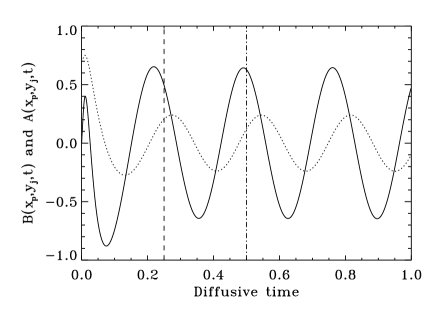
Figure 3.— Representative case for $\alpha_{0}=-0.02665$, $\Omega_{0}=0.03$ and $\eta=0.001$: time evolution of the toroidal field (plain line) and poloidal potential dotted line at a particular point in space (upper panel) and time-latitude cut of the toroidal field at a depth $x_{p}$ near the top of the domain (lower panel). The latter represents the butterfly diagram of our solution. The dashed and dashed-dotted lines represent respectively the end of the first and second assimilation window.

A typical dynamo solution found in our model is shown in Fig. 3. Our set of parameters ($\alpha_{0}=-0.02665$, $\Omega_{0}=0.03$ and $\eta=0.001$) was carefully chosen so that we are in the marginally stable regime. We are exactly at the threshold for which the dynamo instability is triggered, i.e. the growth rate of the instability is purely imaginary and the fields oscillate around zero without growing. If the absolute value of the dynamo numbers were further increased, the dynamo instability would grow and in this linear case, the magnetic energy would increase exponentially without bound.

The lower panel of Fig.3 shows the butterfly diagram, i.e. a time-latitude cut of the toroidal field $B_{z}$ at a particular location in depth. Again, our choice of parameters, especially the sign of the dynamo number $C_{\alpha}C_{\Omega}$ was made to produce an equatorward propagating dynamo wave. Indeed, Yoshimura (1975) showed that the direction of propagation of the dynamo wave when a radial shear is present depends on the sign of the product $\alpha_{0}\Omega_{0}$.

2.3. Generating observational data

The idea of this work is to show that data assimilation techniques can be applied to solar dynamo models. To do so, we develop the adjoint model necessary for the variational assimilation described in Section 1 and we test its validity. We will generate synthetic observations with a certain set of parameters and will use our adjoint model to minimize the cost function and recover the right parameters starting from a random initial guess. Such a procedure is called a twin experiment and has been used in various situations and studies before (e.g. Fournier et al., 2007, ).

We choose as our synthetic data the dynamo solution presented in the previous section. In our twin experiments, the observations are chosen to be the toroidal field $B_{z}$ at $ny$ specific points in space and $nt$ points in time, corresponding in the Sun to the value of the sunspots magnetic field at different latitudes and time during the cycle.

The aim of the adjoint procedure will then be to reconstruct the state vector $\hat{\alpha}$, the dimension of which is the number of points in the $y$-direction, fixed to $30$ in all calculations. In the remaining of the paper, we distinguish the true physical ingredient (denoted $\alpha$) and the state vector to be reconstructed (denoted $\hat{\alpha}$).

2.4. Adjoint $\alpha\Omega$ dynamo model

In the appendix, we present the derivation of the continuous adjoint induction equation. This helps us gaining some insight on the relation between the mathematical definition of an adjoint operator and the procedure we are using in this work. However, it has to be pointed out that it is not the adjoint partial differential equation which will be discretized to build the adjoint code. To do so, we rather attribute an adjoint instruction to each direct instruction in the tangent linear model deduced from the linearization of the direct model. This follows the formal procedure described in Talagrand 1991 and Giering & Kaminski 1998 .

The goal of the whole variational experiment here is to minimize a cost function $\cal{J}$ which will measure the misfit between the observations and the values of the variables calculated by the numerical model. To do so, we need first to define a proper cost function which will have to be minimized. Secondly, the idea is to choose a minimization algorithm which uses the values of the cost function (calculated by the direct integration of the model) and its gradient with respect to all input parameters (produced by the adjoint integration).

For our studies, we choose the following cost function

$$\mbox{$\cal{J}$}=\sum_{k=1}^{nt}\,\,\sum_{j=1}^{ny}\,\,\frac{(B_{z}(x_{p},y_{j},t_{k})-B_{z}^{obs}(x_{p},y_{j},t_{k}))^{2}}{\omega(j,k)^{2}}$$ (16)

where $x_{p}$ is a particular depth. It is chosen to be close to the boundary of the domain in our case, in the attempt to get closer to the real Sun where data are available only at the surface. $\omega(j,k)$ can be adjusted to give more or less weights to some observations, if for example some are more reliable than others. This would happen if a new instrument with more accuracy was launched (then we can expect the errors on the observations to vary in time) or if observations of certain regions in space were less subject to uncertainty. In our twin experiments described below, $\omega(j,k)$ is chosen to be constant, i.e. independent on the position in space or time.

The cost function is then minimized through a quasi-Newton method which uses the first and second derivatives of the function. A particularity of the quasi-Newton methods is that they need the gradient of the function (which is here provided by the adjoint integration) but do not require exact computation of the Hessian matrix, which is instead approximated by an iterative algorithm (here the formula of Broyden-Fletcher-Goldfarb-Shanno is used to update the value of the Hessian approximation). See Polak (1971) for details about the algorithm. We note here that the computation of the gradient of the cost function through the adjoint code has been tested. To do so, we checked that the quantity

$$\mbox{$\cal{J}$}(X+\delta X)-\mbox{$\cal{J}$}(X)-\delta X\cdot\nabla\mbox{$\cal{J}$}(X)$$ (17)

with $\nabla\mbox{$\cal{J}$}(X)$ calculated through the adjoint code, is order $o(\delta X)$ to computer accuracy.

3. Twin experiments and results

As discussed in Sect.2.3, we wish to reconstruct the true state $\alpha$. To do so, we perform several experiments to assess the sensitivity and quality of the reconstructed state.

3.1. Regular sampling in space

Our first experiment consists in producing data with the choice of parameters quoted above at regularly-spaced locations in space and time. More specifically, we fix the value for the $x$-coordinate (representing the depth in the convection zone) and we produce observations both in the Northern and Southern hemispheres, with a regular spacing. Moreover, those observations will be available during the first cycle(s) only, with a regular spacing in time.

The initial guess is $\hat{\alpha}=0$ on every grid points except at the boundaries $y=-1$ and $y=1$ where $\hat{\alpha}$ is set to the true state. Indeed, the values of $\hat{\alpha}$ at the boundaries will not affect our cost function since the magnetic field $B_{z}$ is exactly set to zero at those points (see lower panel of Fig.3 and Eqs.10 and 11). As a consequence, in the minimization procedure, only $\hat{\alpha}$ within the domain is adjusted to reduce the amplitude of the cost function. The tolerance on the gradient is set to $10^{-12}$, which is typically reached after about 300 iterations of our minimization algorithm. By that time, depending on the number of observations used, the final value of the cost function varies between $10^{-17}$ and $10^{-27}$, i.e. has decreased by at least 16 orders of magnitude. We note here that the number of iterations might seem large compared to the dimension of the state vector. However, close to both the boundaries and the equator, the amplitude of the toroidal field $B_{z}$ is about 100 times smaller than at mid-latitude. Since the $\hat{\alpha}$ function only affects the cost function through its product with $B_{z}$ (see Eqs. 10 and 11), the recovery of $\hat{\alpha}$ will be less efficient in the regions where $B_{z}$ is close to zero. If, on the contrary, those points are removed from the assimilation procedure and initially set to their true values, the convergence is much faster (not shown). We will discuss the difficulties of recovering $\hat{\alpha}$ in the equatorial regions in the following sections.

Figure 4.— Initial guess and $\hat{\alpha}$ recovered by the minimization of the cost function with 10 observations in time and 10 regularly spaced observations along the y-direction for each of those 10 points in time. We also show the error between the recovered $\hat{\alpha}$ and the true state, magnified by a factor $10^{7}$.

We run our minimization procedure and compare the results obtained when various numbers of observations are assimilated. The number of points in time can be 5 or 10, located in the first or first two cycles (see the 2 assimilation windows in Fig.3). In space (more specifically in the direction of $y$, representing the latitude), the number of observations varies from 6 to 14. The total number of observations thus extends from 30 to 140 depending on the calculation. Figure 4 shows a typical result of the minimization algorithm for 100 assimilated observations. The function is perfectly recovered and the pointwise error has been reduced by a factor $10^{7}$ compared to the initial guess.

The first conclusion which can be drawn from this experiment is that, as must necessarily be, increasing the number of observations decreases the error made on the reconstructed $\hat{\alpha}$ (see Fig.5). However, even 30 observations in total (5 in time times 6 in space) are sufficient to get an $\hat{\alpha}$ function indistinguishable from the true state. The only quantitative way to compare the different experiments is thus to look at the $L_{2}$ errors between the $\hat{\alpha}$ coming from the minimization algorithm and the true $\alpha$ used to produced the observations. More precisely, we calculate the following quantity

$$e=\sqrt{\frac{\sum_{j=1}^{ny}\,\,\left(\hat{\alpha}(y_{j})-\alpha(y_{j})\right)^{2}}{\sum_{j=1}^{ny}\,\,\alpha(y_{j})^{2}}}$$ (18)

Figure 5.— $L_{2}$ error on $\hat{\alpha}$ (compared to the $\alpha$ used to produce the observations) for various numbers of observations in space and time. Note the monotonous decrease in the error when 10 points in time are used as observations.

The amplitude of those errors are shown in Fig. 5, as a function of the number of observations in the $y$-direction. For completeness, we show the results obtained when observations are located both in the first cycle ($nt=5$) and in the first two cycles ($nt=10$). We clearly show here that the error almost monotonically drops when more and more observations are assimilated, reaching values of the order of $10^{-7}$ for the best cases. The reconstructed $\hat{\alpha}$ then produces poloidal and toroidal magnetic fields very much in agreement with our synthetic observations, as shown in Fig. 6.

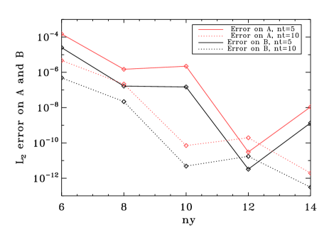
Figure 6.— $L_{2}$ errors on the toroidal (black lines) and poloidal fields (red lines) for the different experiments.

Figure 6 shows the $L_{2}$ errors, on the toroidal and poloidal fields produced by the reconstructed $\hat{\alpha}$ effect, for various numbers of assimilated observations. Again, we find a very good agreement both for the poloidal and toroidal fields even for the smallest number of observations. For larger numbers of observations, the relative errors reach values close to $10^{-10}$ and even $10^{-12}$ for the toroidal field. It is interesting to note that the errors on the toroidal field are systematically about one order of magnitude less than the errors on the poloidal field. This is likely due to the fact that observations are available on the toroidal field only (e.g. the cost function depends exclusively on $Bz$) and thus a better agreement is to be expected. We can also note on this figure that the errors do not grow in time and thus that the functions are recovered on the whole time interval, even if observations were only available on the first cycles. This feature is mainly due to the fact our system of equations is stable to perturbations of the initial conditions, meaning that an initial perturbation would not be amplified nor damped.

Figure 7.— Gradient of $\cal{J}$ with respect to $\hat{\alpha}$ in the case where observations (represented by the squares at the bottom of the graph) are regularly spaced in $y$. The various curves represent the value of the gradient after 30 iterations of the minimization algorithm, $50\times\nabla\mbox{$\cal{J}$}$ after 100 iterations, $500\times\nabla\mbox{$\cal{J}$}$ after 160 iterations and $10000\times\nabla\mbox{$\cal{J}$}$ after 200 iterations.

For the best case considered ($nt=10$, $ny=14$), we found it instructive to follow the evolution of the gradient of the cost function with respect to $\hat{\alpha}$ during the minimization procedure. We choose particular steps in the iterative minimization procedure, separated by sufficiently large decreases of the norm of the gradient. The results are shown in Fig.7 where the gradient is plotted at those steps, with respect to the y-coordinate. The first thing we note is the clear decrease in the amplitude from the beginning to the end of the procedure, the last step chosen (after 200 iterations) being very close to the total number of iterations required to achieve convergence (211 in this case). The second striking property of the curves shown on this figure is the shape of the function, antisymmetric with respect to the equator. This characteristic indicates that the cost function $\cal{J}$ is not sensitive to the values of $\hat{\alpha}$ close to the equator and explains why the difficulties to reproduce the true $\alpha$-effect lie mostly in the equatorial regions. This will be even more obvious in the following sections where data are chosen not to be distributed over the whole domain or when data are perturbed by a random noise. However, the profile of the gradient is not surprising if we consider Eq. B16 of Appendix B and Eqs. 10 and 11, that clearly demonstrate that if $B_{z}$ is zero, $\hat{\alpha}$ has no influence in the equation for the magnetic field. Stated otherwise, the profile of $\nabla_{\alpha}\mbox{$\cal{J}$}$ follows that of the mean value of $B_{z}$ over the time interval in which the assimilation procedure is applied. As a test, we plotted $<B_{z}(x,y)>_{t}$ with respect to $y$ at a particular point in $x$ (not shown) and indeed, we recovered the exact same profile as what is shown in Fig.7 for the various curves.

3.2. Irregular sampling in space

We chose here as observations a quantity $B_{z}$ related to the intensity of the sunspots magnetic field. In the real Sun, sunspots emerge at mid-latitudes at the beginning of the magnetic cycle and closer and closer to the equator as the cycle proceeds. For a more realistic experimental setting, we have studied different cases for which we have assimilated observations in restricted latitudinal bands. We first show the results of an experiment where data were available in one hemisphere only and in the next section, we investigate the case where observations are assimilated in the activity belt only, i.e. at low latitudes in both hemispheres.

3.2.1 One hemisphere only sampling

In this first case, we produce synthetic data only in the Southern hemisphere (for negative values of $y$) and study the reconstruction of the $\hat{\alpha}$ function through the minimization algorithm. Again, the initial guess is $0$ everywhere except on the boundaries and observations are equally spaced in time and on the first two cycles only (10 points in time are used here).

Figure 8.— Upper panel: $\hat{\alpha}$ reconstructed after assimilation of data in the Southern hemisphere only, with 2 different sets of observations, superimposed with the true state. Lower panel: Errors made on the reconstructed $\hat{\alpha}$ for the initial guess (see Fig. 2) and after assimilation of the 2 sets of observations.

Figure 8 shows the results of the minimization. It is clear that where data have been assimilated, the reconstruction of the function is much more accurate than on the Northern hemisphere where observations were absent. The behavior of the function is much smoother in the Southern hemisphere and very similar for both sets of observations. On the contrary, the function strongly fluctuates on the data-free region and especially in the equatorial region for the experiment where only 10 points in space were used. However, when observations are added mostly close to the equatorial region, the error is reduced even on the data-free region and the equatorial region is almost correctly recovered.

Figure 9.— Gradient of $\cal{J}$ with respect to $\hat{\alpha}$ in the case where observations (represented by the filled squares at the bottom of the graph) are available only in one hemisphere. The various curves represent the value of the gradient after 30 iterations of the minimization algorithm, $80\times\nabla\mbox{$\cal{J}$}$ after 100 iterations, $2000\times\nabla\mbox{$\cal{J}$}$ after 400 iterations and $20000\times\nabla\mbox{$\cal{J}$}$ after 990 iterations.

However, even if there exists a clear asymmetry between the two hemispheres here, it has to be noted that the error on the $\hat{\alpha}$ function after minimization is much less than the initial error, even in the data-free region. This is shown on the lower panel of Fig. 8, where the pointwise error is plotted for the initial guess and for the recovered $\hat{\alpha}$. We thus conclude from those experiments that a knowledge of the toroidal field only in one hemisphere also gives us some information on the profile of the $\alpha$-effect in the other hemisphere. This result shows that a link exists between the two hemispheres, due to various physical processes, explaining why the intensity of the magnetic field in one hemisphere will influence the other hemisphere. In the Sun, this link could be related to magnetic flux crossing the equator at particular moments during the cycle or to the dipolar topology of the poloidal field.

Again, as in the previous section, we have followed the evolution of the gradient of the cost function with respect to $\hat{\alpha}$. Various instants in the minimization algorithm were chosen, namely after 30, 100, 400 and 990 iterations (the larger number of iterations being due to the slower convergence of the algorithm). At the beginning of the minimization procedure, an asymmetry between the two hemispheres is clearly visible, as can be expected. This is seen in the analysis of the full curve of Fig.9, which represents the gradient after 30 iterations of the algorithm. The peak value of the gradient in the Southern hemisphere is here about 3 times higher than the peak value in the Northern hemisphere. However, as the minimization proceeds, the gradient in the Southern hemisphere is reduced more than in the Northern hemisphere, leading to a more and more symmetric profile with respect to the equator.

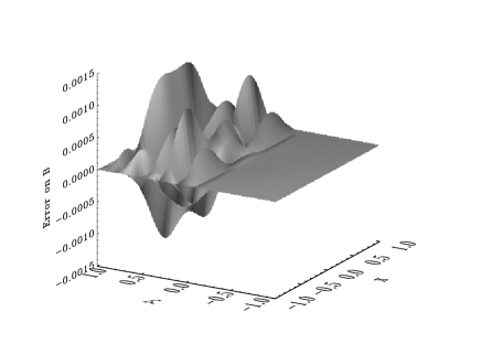
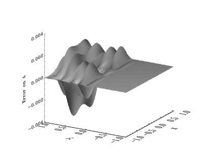
Figure 10.— Difference between the components of the toroidal magnetic field (upper panel) and poloidal potential (lower panel) produced by the reconstructed $\hat{\alpha}$ and the true state at t=0.5 (in the middle of the time interval).

Once again, we can analyze the quality of the magnetic fields produced by the reconstructed $\hat{\alpha}$ and calculate its errors compared to the true state. This is shown in Fig. 10 at one instant, for the case where 8 observations were used. We wish here to focus on the errors at a particular instant in the simulation since we are interested in the spatial distribution of the error, rather than on its time evolution. We show on this figure that again the field is in very good agreement with the true state in the region where observations were assimilated, the relative errors reaching values as low as $10^{-6}$ in these regions. On the contrary, the agreement in the Northern hemisphere is much worse, even if the relative error is of the order of $10^{-3}$ for the toroidal field. For the poloidal field, the errors are again almost one order of magnitude higher, still due to the fact that observations are available on the toroidal field only. We should note that the agreement for the poloidal field on the Southern hemisphere is very satisfactory, stressing the efficiency of the variational assimilation.

3.2.2 Active latitude band sampling

If we choose as observations the sunspot magnetic field detected during solar cycles, we have to be aware that observations will mainly be available in the solar activity belt, i.e. between about $-35^{o}$ and $35^{o}$ in latitude (Hathaway 2010).

Figure 11.— Errors made on the reconstructed $\hat{\alpha}$ after assimilation of various numbers of observations located in the equatorial regions, between $-35^{o}$ and $35^{o}$ for the broadest interval.

We thus choose to investigate the recovery of our true state in a case where data are assimilated close to the equator only.

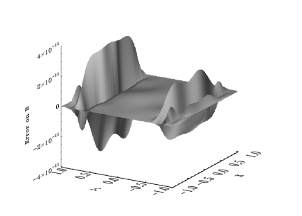
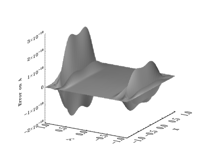
Figure 12.— Same as Fig. 10 but for a case where data are assimilated in the equatorial region only between $-35^{o}$ and $35^{o}$.

Figure 11 shows the results of various experiments where data have been assimilated in a more or less narrow band around the equator. We present cases where observations have been produced successively between $-18^{o}$ and $18^{o}$, $-26^{o}$ and $26^{o}$ and $-35^{o}$ and $35^{o}$. Figure 11 shows the difference of each reconstructed $\hat{\alpha}$ to the true state. It is quite clear again that the recovery of the correct $\hat{\alpha}$ is optimal at the locations where observations were present. Indeed, the function is very smooth and close to the true state at low latitudes for the first two runs. Close to the poles, the fluctuations around the true $\hat{\alpha}$ can be quite significant, the error being there of the same order as the function itself for the first run. However, when the area spanned by the observations increases, the agreement with the true state improves and when observations between about $-35^{o}$ and $35^{o}$ in latitude are used, the relative error made on $\hat{\alpha}$ is as low as $10^{-7}$. This is an interesting property since the actual activity band in the Sun is approximately located within those latitudes. We note in this particular case that the errors are of the same order everywhere in the domain and that the difference of knowledge/information between the region where data were available and the poles is mostly absent. We conclude here that the whole function has been recovered to a very good accuracy for this case where data were assimilated only in the activity belt.

Once again, we can check the results on the magnetic fields produced by the recovered $\hat{\alpha}$. Results are shown in Fig. 12. We chose to show the results for the assimilation on the latitudinal band $-35^{o}$ to $35^{o}$ since the resulting $\hat{\alpha}$ function for this case was recovered to a very good and similar accuracy in the whole domain. The largest errors both on the poloidal and toroidal fields at one instant are again located mainly in the data-free regions. Nevertheless, we note that their amplitude remains very small, even in the polar regions. Again, the errors on the poloidal field (for which we do not produce observations) are about one order of magnitude larger than those on the toroidal field. It has to be noted here that the difference of knowledge/information between the equator and the poles is visible, contrary to what we found for the recovered $\hat{\alpha}$, stressing the not so direct correspondence between the $\alpha$-effect and the magnetic field evolution. The recovery within the equatorial band is excellent, the error reaching values close to $10^{-12}$ for the toroidal field and $10^{-11}$ for the poloidal field.

3.3. Additional noise on the observed data

In reality, the assimilated observations will always be contaminated by errors. Hence, it is natural to study the behavior of our assimilation technique when observations depart significantly from what is directly produced by the numerical model. To do so, we produce the same synthetic data by running the direct code once with the choice of parameters quoted in sect.2.2. We then add noise on the data by calculating

$${B_{z}}_{noise}^{obs}=B_{z}^{obs}*(1+\sigma\,r)$$ (19)

$r$ being a random number between $-1$ and $1$ and $\sigma$ measuring the departure from the synthetic data produced by the direct code.

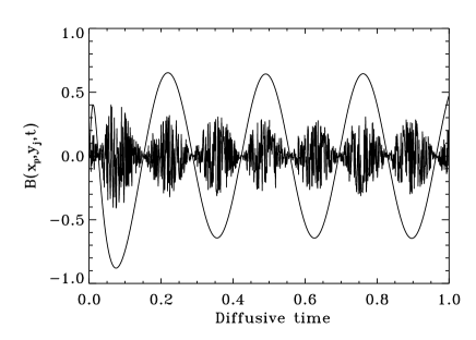
Figure 13.— True state (smooth plain line) and error introduced in the data (magnified by a factor 50, fluctuating line) which will be used for the assimilation. This is a special case where the synthetic data have been perturbed by a noise with a standard deviation of $\sigma=10^{-2}$.

As an illustration, we show in Fig. 13 the time evolution of the “true” toroidal field at a specific point in space. We superimpose the error on ${B_{z}}_{noise}^{obs}$ and the true state for $\sigma=10^{-2}$, magnified by a factor 50. As a direct consequence of Eq. 19, the noise is proportional to the value of $B_{z}$ and thus the errors are higher at periods of maximal activity.

The results of the assimilation procedure are shown in Fig. 14. The number of observations used here was 100 (10 in time multiplied by 10 in the y-direction). With the unperturbed synthetic observations, the assimilation of those particular observations gave us an $L_{2}$-error on $\alpha$ of about $6\times 10^{-8}$ and between $10^{-11}$ and $10^{-12}$ for the magnetic fields (see figures 5 and 6). We will thus be able to directly compare the results of the minimization after assimilation of perturbed and unperturbed data. Four different experiments were investigated, three of which are represented in Fig. 14. The only difference between those various experiments is the coefficient of the observation error $\sigma$.

Figure 14.— Reconstructed $\alpha$ after assimilation of data perturbed with random noises with various standard deviations. 100 observations were used (10 in time and 10 along the y-direction).

From the figure, it is clear that the minimization of the cost function gives $\hat{\alpha}$ profiles which agree less and less with the true state when the noise on the assimilated data is increased. More precisely, when $\sigma=10^{-5}$, the $\hat{\alpha}$ function is almost perfectly recovered, except from a small region around the equator in which the cost function is less sensitive to the values of $\hat{\alpha}$. When $\sigma=10^{-4}$, the result of the minimization procedure gives an $\hat{\alpha}$ which is already much less satisfactory, the $L_{2}$-error to the true state being of the order of $10^{-1}$ (compared to $6\times 10^{-8}$ for the unperturbed case). When $\sigma$ is further increased, the recovery of the $\hat{\alpha}$ profile is poor, the error being of about $50\%$ in this case. The final errors on the toroidal and poloidal magnetic fields are of the same order as the errors introduced on the assimilated data, which shows that the minimization is fundamentally successful. Nevertheless, even if the true state and the final fields depart of the same amount from the perturbed observations, the errors between them are still significant. For $\sigma=10^{-5}$, the minimum $L_{2}$-error reached on $B_{z}$ is of the order of $4\times 10^{-5}$, about 6 orders of magnitude higher than the typical errors in similar situations using unperturbed data.

4. Conclusion

We have presented the first attempt to apply variational data assimilation techniques to the solar dynamo. A very simplified formulation was used, namely a linear deterministic $\alpha\Omega$ dynamo model in Cartesian geometry, which should not be taken as an accurate representation of the magnetic field regeneration and evolution in the Sun. Nevertheless, we showed that with this simple model, variational data assimilation gives us a way to constrain various input parameters such as the profile of the $\alpha$-effect, through the minimization of the errors to very few observations (140 observations at most were used, out of 30000 points in the (y,t) plane). With regularly-spaced observations, the variational technique enabled us to recover the profile of the $\alpha$-effect at the accuracy of about $10^{-8}$, starting from an initial guess with an error of $10^{-2}$. This recovered $\alpha$ then produced magnetic fields in extremely good agreement (accuracy of around $10^{-12}$) with the true state.

Moreover, we showed that a partial knowledge of the toroidal field could give us useful information on the $\alpha$-effect in the whole domain. Indeed, we showed that assimilating data in the latitudinal belt of activity (between $-35^{o}$ and $35^{o}$) is enough to reconstruct $\alpha$ at all latitudes with a final $L_{2}$-error of $10^{-7}$. We also showed that adding noise on the observations strongly perturbed the results of the minimization procedure, even if the global shape of the $\alpha$-effect was mainly recovered in all cases (and especially the antisymmetry about the equator). Finally we showed that the reconstruction of the $\alpha$-effect in our toy model is difficult near the equator if the observed (generated) data assimilated in the procedure are insensitive to variations in that region, as it was the case here with $B_{z}$ being zero. However, if we had considered an $\alpha^{2}\Omega$ dynamo model (with the $\alpha$-effect present in the production of $B_{z}$), that comment might have not been true. This will be checked in future investigations. Other quantities such as the differential rotation or observed variables such as the poloidal field could help better reconstructing information in these specific locations. It may then be worth trying several combinations of quantities and variables in our attempt to better determine the internal dynamics of the Sun.

The proof of concept presented in this work is very promising for the future developments of solar magnetic activity forecast. Indeed, we showed that if a physical model is assumed to be sufficiently close to reality, the knowledge of a very small piece of information could provide us with the reconstruction of a very important physical process for which direct measurements are not available. More precisely, in the case of the Sun, if we assume that the meridional flow (large-scale flow in the meridional plane) plays a significant role in the evolution of the large-scale magnetic field Dikpati & Gilman 2006 ; Jouve & Brun 2007 ; Nandy et al. 2011 and hence in the dynamo loop, data assimilation could be very useful. Indeed, the meridional circulation is very difficult to measure accurately, especially at depths higher than a few tens of Mm (see review of Miesch 2005 and recent observations of Hathaway & Rightmire 2010). However, the magnetic field strength and configuration now start to be detected with great accuracy through new satellites as Hinode and SDO that provide vector magnetograms of the full solar disk. Data assimilation is then a way to link the direct measurements of, say, the radial field in active regions and a physical model in which the meridional flow takes part in the dynamo loop. It is the case for instance of flux-transport dynamo models which are sometimes used to model the whole evolution of large-scale magnetic fields in the Sun. Not only would some subtle physical processes (i.e. difficult to detect directly) be reconstructed through the assimilation of accurate observations of more accessible variables, but we could then use the physical models to predict the behavior of the next solar cycle, with a different technique from what was used up to now.

We said in the introduction that a reliable technique to predict future solar magnetic phenomena still does not exist, we propose here a way to progress in this direction, inspired by what has been used for a long time already in the Earth weather community. Of course, better physical models and better understanding of the physical processes interacting in a star need to be developed before we can safely apply data assimilation techniques to give tentative predictions of the solar activity. In particular, the goal would be to assimilate observations of excellent quality (which are already available) in 3D MHD global solar dynamo models producing realistic magnetic cycles (which are not yet available). In the meantime, we try to progress step by step towards this goal and we think this work constitutes one of these steps, proving the possibility to apply modern data assimilation techniques in solar physics. A next step could be to use a nonlinear dynamo model that is sensitive to the initial conditions and which uses polar coordinates rather than Cartesian ones. Finally, we could also introduce a so-called background term in the cost function, which limits the departure from an a priori estimate of the state vector (see Fournier et al. 2010, , for further details). This allows to introduce data that is not contained in the observations such as information on the smoothness of the physical parameters (like the function $\alpha$ for example). We intend to do so in the near future.

Appendix A The adjoint induction equation

In this section, we present in details the different steps leading to the determination of the continuous adjoint mean-field induction equation. This is only of particular use for the development of the adjoint model but we find it useful to gain some insight on the link between adjoint operators and the calculations shown in this work.

The velocity field ${\bf v}$, magnetic diffusivity $\eta$ and the $\alpha$-effect are given functions of space and time. We show here how to compute the adjoint of each operator appearing in the equation. We first define the adjoint operator in the following manner:

$\Psi^{\star}$ is the adjoint of $\Psi$ operating on the Euclidian space $E$ if and only if

$$\forall({\bf u_{1}},{\bf u_{2}})\in E^{2},\,\,\,\,\Psi({\bf u_{1}})\cdot{\bf u_{2}}={\bf u_{1}}\cdot\Psi^{\star}({\bf u_{2}})$$ (A1)

where $\cdot$ is the scalar product on $E$. As a consequence, in order to determine the adjoint of an operator, we need to find the operator such that condition A1 is fulfilled.

Let ${\bf u_{1}}$ and ${\bf u_{2}}$ be elements of the Euclidian space $E$.

1. We first try to get the adjoint of the operator ${\bf u}\rightarrow{\bf v}\times{\bf u}$. Let $\Psi^{\star}$ be such that $({\bf v}\times{\bf u_{1}})\cdot{\bf u_{2}}={\bf u_{1}}\cdot\Psi^{\star}({\bf u_{2}})$. Then by manipulation of vector identities, we get:

$$({\bf v}\times{\bf u_{1}})\cdot{\bf u_{2}}=-{\bf u_{1}}\cdot({\bf v}\times{\bf u_{2}})$$ (A2)

The adjoint of ${\bf u}\rightarrow{\bf v}\times{\bf u}$ is thus ${\bf u}\rightarrow-{\bf v}\times{\bf u}$.

2. Let us now look for the adjoint of ${\bf u}\rightarrow\nabla\times{\bf u}$. Let $\Psi^{\star}$ be such that $(\nabla\times{\bf u_{1}})\cdot{\bf u_{2}}={\bf u_{1}}\cdot\Psi^{\star}({\bf u_{2}})$.

$$(\nabla\times{\bf u_{1}})\cdot{\bf u_{2}}={\bf u_{1}}\cdot(\nabla\times{\bf u_{2}})+\nabla\cdot({\bf u_{1}}\times{\bf u_{2}})$$ (A3)

The adjoint of ${\bf u}\rightarrow\nabla\times{\bf u}$ is thus ${\bf u}\rightarrow\nabla\times{\bf u}$, the term $\nabla\cdot({\bf u_{1}}\times{\bf u_{2}})$ representing a boundary term which will be used in the adjoint integration to test the sensitivity of the cost function to the boundary conditions for example.

3. W e now determine the adjoint of ${\bf u}\rightarrow\alpha{\bf u}$ Let $\Psi^{\star}$ be such that $(\alpha{\bf u_{1}})\cdot{\bf u_{2}}={\bf u_{1}}\cdot\Psi^{\star}({\bf u_{2}})$. It is straightforward to see that

$$(\alpha{\bf u_{1}})\cdot{\bf u_{2}}={\bf u_{1}}\cdot(\alpha{\bf u_{2}})$$ (A4)

The adjoint of ${\bf u}\rightarrow\alpha{\bf u}$ is thus ${\bf u}\rightarrow\alpha{\bf u}$ (this operator is said to be self-adjoint).

4. Finally, we need to get the adjoint of ${\bf u}\rightarrow\partial{\bf u}/\partial t$. Let $\Psi^{\star}$ be such that $\partial{\bf u_{1}}/\partial t\cdot{\bf u_{2}}={\bf u_{1}}\cdot\Psi^{\star}({\bf u_{2}})$. We have:

$$\frac{\partial{\bf u_{1}}}{\partial t}\cdot{\bf u_{2}}=-{\bf u_{1}}\cdot\frac{\partial{\bf u_{2}}}{\partial t}+\frac{\partial({\bf u_{1}}\cdot{\bf u_{2}})}{\partial t}$$ (A5)

The adjoint of ${\bf u}\rightarrow\partial{\bf u}/\partial t$ is thus ${\bf u}\rightarrow-\partial{\bf u}/\partial t$, the term $\frac{\partial({\bf u_{1}}\cdot{\bf u_{2}})}{\partial t}$ now representing an initial conditions term which could be used the adjoint integration to study the effect of the initial conditions on a particular cost function.

We are thus able now to write the adjoint induction equation, using the property that the adjoint of a composition of operators is the compositions of the adjoint operators, taken in the reverse order.

Finally, we have:

$$\frac{\partial{\bf B}}{\partial t}={\bf v}\times(\nabla\times{\bf B})-\alpha\nabla\times{\bf B}+\nabla\times(\eta\nabla{\bf\times B})$$ (A6)

Appendix B Variational approach

In this section we will follow and adapt the procedure described in Talagrand 2003 . Let’s consider the coupled induction equations 10 and 11 for the fields $A$ and $B_{z}$. We search solutions of this set of equations over the rectangular domain $D=[x_{1},x_{2}]\times[y_{1},y_{2}]\times[t_{1},t_{2}]$ in (x,y,t)-space. These equations are first order with respect to $t$ and second order with respect to $x$ and $y$.

Consider now a field $B_{z}^{obs}(x,y,t)$ of observations over the domain $D$. Since we assimilate data only on the toroidal field (as a proxy of the surface sunspots) our cost function $\cal{J}$ is written:

$$\mbox{$\cal{J}$}(B)=\frac{1}{2}\iiint\limits_{D}(B_{z}-B_{z}^{obs})^{2}\,dxdydt$$ (B1)

its variation is thus:

$$\delta\mbox{$\cal{J}$}=\iiint\limits_{D}(B_{z}-B_{z}^{obs})\delta B_{z}\,dxdydt$$ (B2)

We aim at expressing the variations of the cost function $\cal{J}$ to variations of our well-defined input parameters which are:

• The values of $A$ and $B_{z}$ for all points in space at the initial time $t=t_{1}$

• The constant magnetic diffusivity $\eta$

• The function representing the $\alpha$-effect $\alpha(x,y)$

• The azimuthal velocity function $v(x,y)$

Let’s derive the tangent linear equation obtain by differentiating equations 10 and 11 with respect to $A$, $B_{z}$, the parameter $\eta$ and the functions $v$ and $\alpha$ and name respectively their variations $\delta A$, $\delta B_{z}$, $\delta\eta$, $\delta v$, $\delta\alpha$. The equations read:

$$\frac{\partial\delta A}{\partial t}-\delta\alpha B_{z}-\alpha\delta B_{z}-\eta(\frac{\partial^{2}\delta A}{\partial x^{2}}+\frac{\partial^{2}\delta A}{\partial y^{2}})-\delta\eta(\frac{\partial^{2}A}{\partial x^{2}}+\frac{\partial^{2}A}{\partial y^{2}})=0$$ (B3)

$$\frac{\partial\delta B_{z}}{\partial t} - \frac{\partial\delta v}{\partial x}\frac{\partial A}{\partial y}+\frac{\partial\delta v}{\partial y}\frac{\partial A}{\partial x}-\frac{\partial v}{\partial x}\frac{\partial\delta A}{\partial y}+\frac{\partial v}{\partial y}\frac{\partial\delta A}{\partial x}$$ (B4)

$$- \eta(\frac{\partial^{2}\delta B_{z}}{\partial x^{2}}+\frac{\partial^{2}\delta B_{z}}{\partial y^{2}})-\delta\eta(\frac{\partial^{2}B_{z}}{\partial x^{2}}+\frac{\partial^{2}B_{z}}{\partial y^{2}})=0$$

Using Lagrange multipliers $\lambda(x,y,t)$ and $\gamma(x,y,t)$ respectively for equations B3 and B4, we get (introducing a negative sign for simplicity):

$$\delta\mbox{$\cal{J}$}=\iiint\limits_{D}\left((B_{z}-B_{z}^{obs})\delta B_{z}-\lambda\left[\frac{\partial\delta A}{\partial t}-\delta\alpha B_{z}-\alpha\delta B_{z}-\eta(\frac{\partial^{2}\delta A}{\partial x^{2}}+\frac{\partial^{2}\delta A}{\partial y^{2}})\right.\right.$$

$$\left.-\delta\eta(\frac{\partial^{2}A}{\partial x^{2}}+\frac{\partial^{2}A}{\partial y^{2}})\right]-\gamma\left[\frac{\partial\delta B_{z}}{\partial t}-\frac{\partial\delta v}{\partial x}\frac{\partial A}{\partial y}+\frac{\partial\delta v}{\partial y}\frac{\partial A}{\partial x}-\frac{\partial v}{\partial x}\frac{\partial\delta A}{\partial y}+\frac{\partial v}{\partial y}\frac{\partial\delta A}{\partial x}\right.$$ (B5)

$$\left.\left.-\eta(\frac{\partial^{2}\delta B_{z}}{\partial x^{2}}+\frac{\partial^{2}\delta B_{z}}{\partial y^{2}})-\delta\eta(\frac{\partial^{2}B_{z}}{\partial x^{2}}+\frac{\partial^{2}B_{z}}{\partial y^{2}})\right]\right)\,dxdydt$$

We now wish to remove all the differentiation operating on $A$, $B_{z}$, $\eta$, $v$ and $\alpha$. To do so we use as many integration by parts as necessary. for the sake of clarity we demonstrate the procedure for a few typical terms:

$$-\iiint\limits_{D}\lambda\frac{\partial\delta A}{\partial t}\,dxdydt=-\int_{x_{1}}^{x_{2}}\int_{y_{1}}^{y_{2}}\lambda\delta A\,dxdy\mbox{\huge$|$}_{t_{1}}^{t_{2}}+\iiint\limits_{D}\frac{\partial\lambda}{\partial t}\delta A\,dxdydt$$ (B6)

Diffusion terms require a double integration by parts:

$$\iiint\limits_{D}\lambda\eta\frac{\partial^{2}\delta A}{\partial x^{2}}\,dxdydt = \int_{y_{1}}^{y_{2}}\int_{t_{1}}^{t_{2}}\lambda\eta\frac{\partial\delta A}{\partial x}\,dydt\mbox{\huge$|$}_{x_{1}}^{x_{2}}-\iiint\limits_{D}\frac{\partial(\lambda\eta)}{\partial x}\frac{\partial\delta A}{\partial x}\,dxdydt$$ (B7)

$$= \int_{y_{1}}^{y_{2}}\int_{t_{1}}^{t_{2}}\lambda\eta\frac{\partial\delta A}{\partial x}\,dydt\mbox{\huge$|$}_{x_{1}}^{x_{2}}-\int_{y_{1}}^{y_{2}}\int_{t_{1}}^{t_{2}}\frac{\partial(\lambda\eta)}{\partial x}\delta A\,dydt\mbox{\huge$|$}_{x_{1}}^{x_{2}}$$

$$+ \iiint\limits_{D}\frac{\partial^{2}(\lambda\eta)}{\partial x^{2}}\delta A\,dxdydt$$

We note that the double integration modifies the sign of the diffusion term relative to the time derivative, this is expected since by going backward in time we should anti-diffuse.

$$-\iiint\limits_{D}\gamma\frac{\partial v}{\partial y}\frac{\partial\delta A}{\partial x}\,dxdydt=-\int_{y_{1}}^{y_{2}}\int_{t_{1}}^{t_{2}}\gamma\frac{\partial v}{\partial y}\delta A\,dydt\mbox{\huge$|$}_{x_{1}}^{x_{2}}+\iiint\limits_{D}\frac{\partial}{\partial x}(\gamma\frac{\partial v}{\partial y})\delta A\,dxdydt$$ (B8)

Terms involving variations of the ingredients are treated likewise:

$$-\iiint\limits_{D}\gamma\frac{\partial A}{\partial x}\frac{\partial\delta v}{\partial y}\,dxdydt=-\int_{x_{1}}^{x_{2}}\int_{t_{1}}^{t_{2}}\gamma\frac{\partial A}{\partial x}\delta v\,dxdt\mbox{\huge$|$}_{y_{1}}^{y_{2}}+\iiint\limits_{D}\frac{\partial}{\partial y}(\gamma\frac{\partial A}{\partial x})\delta v\,dxdydt$$ (B9)

Applying systematically this method to all the terms that possess differentiation of the variations and grouping the terms by variations, we get for $\delta\mbox{$\cal{J}$}$ the following equation:

$$\delta\mbox{$\cal{J}$}=\iiint\limits_{D}\left(\left[\frac{\partial\lambda}{\partial t}+\eta(\frac{\partial^{2}\lambda}{\partial x^{2}}+\frac{\partial^{2}\lambda}{\partial y^{2}})+\frac{\partial}{\partial x}(\gamma\frac{\partial v}{\partial y})-\frac{\partial}{\partial y}(\gamma\frac{\partial v}{\partial x})\right]\delta A\right.$$

$$\left.+\left[\frac{\partial\gamma}{\partial t}+\lambda\alpha+\eta(\frac{\partial^{2}\gamma}{\partial x^{2}}+\frac{\partial^{2}\gamma}{\partial y^{2}})+(B_{z}-B_{z}^{obs})\right]\delta B_{z}+\delta\alpha\lambda B_{z}\right.$$

$$\left.+\delta\eta\left[\lambda(\frac{\partial^{2}A}{\partial x^{2}}+\frac{\partial^{2}A}{\partial y^{2}})+\gamma(\frac{\partial^{2}B_{z}}{\partial x^{2}}+\frac{\partial^{2}B_{z}}{\partial y^{2}})\right]\right.$$

$$\left.-\delta v\left[\frac{\partial}{\partial x}(\gamma\frac{\partial A}{\partial y})-\frac{\partial}{\partial y}(\gamma\frac{\partial A}{\partial x})\right]\right)\,dxdydt$$

$$-\int_{x_{1}}^{x_{2}}\int_{y_{1}}^{y_{2}}\lambda\delta A\,dxdy\mbox{\huge$|$}_{t_{1}}^{t_{2}}$$

$$+\int_{y_{1}}^{y_{2}}\int_{t_{1}}^{t_{2}}\left(\eta\left[\lambda\frac{\partial\delta A}{\partial x}-\frac{\partial\lambda}{\partial x}\delta A\right]-\gamma\frac{\partial v}{\partial y}\delta A+\gamma\delta v\frac{\partial A}{\partial y}\right)\,dydt\mbox{\huge$|$}_{x_{1}}^{x_{2}}$$

$$+\int_{x_{1}}^{x_{2}}\int_{t_{1}}^{t_{2}}\left(\eta\left[\lambda\frac{\partial\delta A}{\partial y}-\frac{\partial\lambda}{\partial y}\delta A\right]+\gamma\frac{\partial v}{\partial x}\delta A-\gamma\delta v\frac{\partial A}{\partial x}\right)\,dxdt\mbox{\huge$|$}_{y_{1}}^{y_{2}}$$

$$-\int_{x_{1}}^{x_{2}}\int_{y_{1}}^{y_{2}}\gamma\delta B_{z}\,dxdy\mbox{\huge$|$}_{t_{1}}^{t_{2}}+\int_{y_{1}}^{y_{2}}\int_{t_{1}}^{t_{2}}\eta\left[\gamma\frac{\partial\delta B_{z}}{\partial x}-\frac{\partial\gamma}{\partial x}\delta B_{z}\right]\,dydt\mbox{\huge$|$}_{x_{1}}^{x_{2}}$$

$$+\int_{x_{1}}^{x_{2}}\int_{t_{1}}^{t_{2}}\eta\left[\gamma\frac{\partial\delta B_{z}}{\partial y}-\frac{\partial\gamma}{\partial y}\delta B_{z}\right]\,dxdt\mbox{\huge$|$}_{y_{1}}^{y_{2}}$$ (B10)

This expression is valid for any $\lambda(x,y,t)$ and $\gamma(x,y,t)$. The space-time integral can be cancelled by imposing that $\lambda$ and $\gamma$ verify the following partial differential equations:

$$\frac{\partial\lambda}{\partial t} + \eta(\frac{\partial^{2}\lambda}{\partial x^{2}}+\frac{\partial^{2}\lambda}{\partial y^{2}})+\frac{\partial}{\partial x}(\gamma\frac{\partial v}{\partial y})-\frac{\partial}{\partial y}(\gamma\frac{\partial v}{\partial x})=0$$ (B11)

$$\frac{\partial\gamma}{\partial t} + \lambda\alpha+\eta(\frac{\partial^{2}\gamma}{\partial x^{2}}+\frac{\partial^{2}\gamma}{\partial y^{2}})+(B_{z}-B_{z}^{obs})=0$$ (B12)

We also impose that $\lambda(x,y,t_{2})$ and $\gamma(x,y,t_{2})$ equal zero for any x or y. Further since $A$ and $B_{z}$ are constrained to be equal to zero at the boundary, their variation are zero, and all the terms involving either $\delta A$ and $\delta B_{z}$ in the surface integrals above vanish. For the terms involving derivatives of $\delta A$ and $\delta B_{z}$ we impose that $\lambda$ and $\gamma$ equal zero on boundaries $x=x_{1},x_{2}$ and $y=y_{1},y_{2}$ for any t.

We note that equations B11 and B12 with the conditions on $\lambda$ and $\gamma$ just stated above unambiguously define the functions in the whole domain. Equations B11 and B12 are first-order in time and second-order in space, and define a well-posed problem for backward integration with respect to $t$, because of the positive sign of the diffusion terms. The specification of $\lambda$ and $\gamma$ at the final time $t_{2}$ and along the spatial boundaries $x_{1},x_{2},y_{1}$ and $y_{2}$ therefore unambiguously define the functions $\lambda(x,y,t)$ and $\gamma(x,y,t)$.

Taking into account these various conditions, equation B reduces to:

$$\delta\mbox{$\cal{J}$}=\int_{x_{1}}^{x_{2}}\int_{y_{1}}^{y_{2}}\lambda(x,y,t_{1})\delta A(x,y,t_{1})dxdy+\int_{x_{1}}^{x_{2}}\int_{y_{1}}^{y_{2}}\gamma(x,y,t_{1})\delta B_{z}(x,y,t_{1})dxdy+\int_{x_{1}}^{x_{2}}\int_{y_{1}}^{y_{2}}\left[\delta\alpha\int_{t_{1}}^{t_{2}}\lambda B_{z}dt\right]dxdy\\ +\delta\eta\iiint\limits_{D}\left[\lambda(\frac{\partial^{2}A}{\partial x^{2}}+\frac{\partial^{2}A}{\partial y^{2}})+\gamma(\frac{\partial^{2}B_{z}}{\partial x^{2}}+\frac{\partial^{2}B_{z}}{\partial y^{2}})\right]\,dxdydt-\iiint\limits_{D}\delta v\left[\frac{\partial}{\partial x}(\gamma\frac{\partial A}{\partial y})-\frac{\partial}{\partial y}(\gamma\frac{\partial A}{\partial x})\right]\,dxdydt$$ (B13)

The above equation reveals that the partial derivatives of the objective function $\cal{J}$ with respect to $\eta$, $\alpha(x,y)$, $v(x,y)$, $A(x,y,t_{1})$ and $B_{z}(x,y,t_{1})$ are equal to:

$$\frac{\partial\mbox{$\cal{J}$}}{\partial A}(x,y,t_{1}) = \lambda(x,y,t_{1})\,\mbox{ and }\,\frac{\partial\mbox{$\cal{J}$}}{\partial B_{z}}(x,y,t_{1})=\gamma(x,y,t_{1})$$ (B14)

$$\frac{\partial\mbox{$\cal{J}$}}{\partial\eta} = \iiint\limits_{D}\left[\lambda(\frac{\partial^{2}A}{\partial x^{2}}+\frac{\partial^{2}A}{\partial y^{2}})+\gamma(\frac{\partial^{2}B_{z}}{\partial x^{2}}+\frac{\partial^{2}B_{z}}{\partial y^{2}})\right]\,dxdydt$$ (B15)

$$\frac{\partial\mbox{$\cal{J}$}}{\partial\alpha} = \int_{t_{1}}^{t_{2}}\lambda B_{z}\,dt\,\,\,\,\,,\forall{(x,y)}$$ (B16)

$$\frac{\partial\mbox{$\cal{J}$}}{\partial v} = \int_{t_{1}}^{t_{2}}\left[\frac{\partial}{\partial y}(\gamma\frac{\partial A}{\partial x})-\frac{\partial}{\partial x}(\gamma\frac{\partial A}{\partial y})\right]\,dt\,\,\,\,\,,\forall{(x,y)}$$ (B17)

We here solve a simplified problem by considering that $A$ and $B_{z}$ at $t=t_{1}$ are known (see Talagrand & Courtier 1987, , for discussions about sensitivity to initial conditions).

References

- (1) Archontis, V., Moreno-Insertis, F., Galsgaard, K., & Hood, A. W. 2005, Astrophysical Journal, 635, 1299
- (2) Beer, J., Tobias, S., & Weiss, N. 1998, Solar Physics, 181, 237
- (3) Bélanger, E., Charbonneau, P., & Vincent, A. 2005, Journal of the Royal Astronomical Society of Canada, 99, 133
- (4) Bocquet, M. 2011, Notes de cours du M2 OACOS, de l’ENSTA et de l’Ecole des Ponts ParisTech
- (5) Browning, M. K., Miesch, M. S., Brun, A. S., & Toomre, J. 2006, Astrophysical Journal Letters, 648, L157
- (6) Brun, A.S., Miesch, S.M. & Toomre, J. 2004, ApJ, 614, 1073
- (7) Brun, A. S., Miesch, S.M. & Toomre, J. 2011, Astrophysical Journal, submitted
- (8) Cameron, R., & Schüssler, M. 2007, Astrophysical Journal, 659, 801
- (9) Cattaneo, F., Hughes, D.W., 2001, A&G, 42, 18
- (10) Charbonneau, P., 2005, Living Rev. Solar Phys., 2
- (11) Choudhuri, A. R., Chatterjee, P., & Jiang, J. 2007, Physical Review Letters, 98, 131103
- (12) Cline, K. S. 2003, Ph.D. Thesis
- (13) Daley, R. 1991, Science, 254, 1531
- (14) de Jager & Duhau, S. 2009, JAST, 71, 239
- (15) Dikpati, M., de Toma, G., Gilman, P. A., Arge, C. N., & White, O. R. 2004, Astrophysical Journal, 601, 1136
- (16) Dikpati, M., & Gilman, P. A. 2006, Astrophysical Journal, 649, 498
- (17) Dikpati, M., de Toma, G., & Gilman, P. A. 2006, Geophysical Review Letter, 33, 5102
- (18) Duhau, S. 2003, Solar Physics, 213, 203
- (19) Fan, Y., Abbett, W.P. & Fisher, G. H. 2003, Astrophysical Journal, 582, 1206
- (20) Fournier, A., Eymin, C. & Alboussière, T. 2007, Nonlin. Processes Geophys., 14, 163
- (21) Fournier, A., et al. 2010, Space Sci. Rev., 155, 24
- (22) Giering, R. & Kaminski, T. 1998, ACM Transactions on Mathematical Software, 24, 437
- (23) Hathaway, D. H. 2010, Living review in solar physics, 7, 1, http://solarphysics.livingreviews.org/Articles/lrsp-2010-1/
- (24) Hathaway, D. H., Wilson, R. M., & Reichmann, E. J. 1999, Journal of Geophysical Research, 104, 22375
- (25) Hathaway, D. H., & Wilson, R. M. 2004, Solar Physics, 224, 5
- (26) Hathaway, D. H., & Rightmire, L. 2010, Science, 327, 1350
- (27) Jouve, L., & Brun, A. S. 2007, Astronomy and Astrophysics, 474, 239
- (28) Jouve, L., & Brun, A. S. 2009, Astrophysical Journal, 701, 1300
- Kalnay (2003) Kalnay, E. 2003, Atmospheric Modeling, Data Assimilation and Predictability. Cambridge Press, 341pp.
- (30) Kitiashvili, I., & Kosovichev, A. G. 2008, Astrophysical Journal Letters, 688, L49
- (31) Komm, R., Howe, R., Hill, F., Miesch, M., Haber, D., & Hindman, B. 2007, Astrophysical Journal, 667, 571
- (32) Komm, R., Hill, F., & Howe, R. 2008, Journal of Physics Conference Series, 118, 012035
- (33) Krause, F., & Raedler, K.-H. 1980, Oxford, Pergamon Press, Ltd., 1980. 271 p.
- (34) Le Dimet, F.-X., & Talagrand, O. 1986, Tellus Series A, 38, 97
- (35) Lorenc, A. C. 1981, Monthly Weather Review, 109, 701
- (36) Magara, T., & Longcope, D. W. 2003, Astrophysical Journal, 586, 630
- (37) Miesch, M. S., Elliott, J. R., Toomre, J., Clune, T. L., Glatzmaier, G. A., & Gilman, P. A. 2000, Astrophysical Journal, 532, 593
- (38) Miesch, M. S. 2005, Living Reviews in Solar Physics, 2, 1
- (39) Moffatt, H. K. 1978, Cambridge, England, Cambridge University Press, 1978. 353 p.
- (40) Nandy, D., Muñoz-Jaramillo, A., & Martens, P. C. H. 2011, Nature, 471, 80
- (41) Ossendrijver,M., 2003, Astronomy and Astrophysics Review, 324, 64
- (42) Pevtsov, A. A., & Canfield, R. C. 2001, Journal of Geophysical Research, 106, 25191
- (43) Polak,E. 1971, Computational Methods in Optimization, New York Academic Press, pp.56ff.
- (44) Rempel, M & Dikpati, M., ASPS, 416, 551 in Solar-stellar dynamos as revealed by helio- and asteroseismology, Gong2008/Soho21
- (45) Roth 2009, ASPS, 416, 501, in Solar-stellar dynamos as revealed by helio- and asteroseismology, Gong2008/Soho21
- (46) Schrijver, C. & DeRosa, M. 2003, Solar Physics, 212, 165
- (47) Schwenn, R. 2006, Living Reviews in Solar Physics, 3, 2
- (48) Steenbeck, M., Krause, F., Raedler, K.-H. 1966, Zeitschrift Naturforschung Teil A, 21, 369
- (49) Stix, M., 2002, The Sun: an introduction, Springer
- (50) Svalgaard, L., Cliver, E. W., & Kamide, Y. 2005, Geophysical Review Letter, 32, 1104
- (51) Talagrand, O., & Courtier, P. 1987, Quarterly Journal of the Royal Meteorological Society, 113, 1311
- (52) Talagrand, O. 1991, Automatic Differentiation of Algorithms, Proceedings, A. Griewank and G.G. Corliss, editors, Society for Industrial and Applied Mathematics, Philadelphia
- (53) Talagrand, O. 1997, Assimilation of observations, an introduction. J. Meteorol. SOC.Japan 75, 191-209.
- (54) Talagrand, O. 2003, Data Assimilation for the Earth System, Proceedings, Advanced Study Insitute, Acquafredda di Maratea, Italy, May-June 2002, Kluwer Academic Publishers, Dordrecht, The Netherlands, 37-53
- (55) Yoshimura, H. 1975, Astrophysical Journal, 201, 740
- (56) Wang, Y.-M. & Sheeley, N.R. 1991, ApJ, 375, 761