Adaptive walks and extreme value theory

Abstract

We study biological evolution in a high-dimensional genotype space in the regime of rare mutations and strong selection. The population performs an uphill walk which terminates at local fitness maxima. Assigning fitness randomly to genotypes, we show that the mean walk length is logarithmic in the number of initially available beneficial mutations, with a prefactor determined by the tail of the fitness distribution. This result is derived analytically in a simplified setting where the mutational neighborhood is fixed during the adaptive process, and confirmed by numerical simulations.

The adaptation of a population to a novel environment is a fundamental process of evolutionary biology which continues to attract considerable attention from theoretical Orr2005 as well as experimental Elena2003 perspectives. Adaptation is driven by the occurrence of mutations that are beneficial in the new environment and therefore spread in the population, leading to an increase of fitness over time. This process displays a variety of dynamical patterns Park2010 that depend on the supply of beneficial mutations (governed by the product of population size $M$ and mutation rate $U$) as well as on the structure of the fitness landscape, which encodes how the genetic configuration of an organism (its genotype) affects the number of offspring it will leave in the next generation.

A particularly simple, yet biologically relevant limit of adpative dynamics is the regime of strong selection and weak mutation (SSWM), where mutations are sufficiently rare to be treated as independent events, $MU\ll 1$, and selection is strong enough for deleterious mutations (which decrease fitness) to be unable to spread Gillespie1983 ; Gillespie1984 ; Orr2002 . In the SSWM regime the population is genetically homogeneous most of the time, and its dynamics can be described by a point in the space of genotypes which performs an adaptive walk towards higher fitness. Because of the low mutation rate such a walk is constrained to move by single mutational steps, and it terminates when a local fitness maximum is reached, where no nearest neighbor genotypes are available that would confer higher fitness. Despite its strongly simplified nature, the adaptive walk model is in principle amenable to quantitative tests in microbial evolution experiments Rokyta2005 ; Schoustra2009 ; Rokyta2009 ; Miller2011 .

In the present Letter we study the length of such adaptive walks in a simple model of a rugged fitness landscape, where fitness values $F_{i}$ of genotypes $i$ are assumed to be independent random variables drawn from a common probability density $\rho(F)$. The genotype space is a generalized hypercube formed by sequences of $L$ letters drawn from an alphabet of size $a$, such that each genotype has $N=(a-1)L$ single mutant neighbors Kauffman1987 . The walk is then specified by the transition probability $P_{ij}$ from genotype $i$ to a neighboring genotype $j$ of higher fitness, $F_{j}>F_{i}$. In the SSWM regime $P_{ij}$ is proportional to the fixation probability of the corresponding beneficial mutation, i.e. the probability that it will become dominant rather than going extinct due to demographic fluctuations Kimura1962 ; Patwa2008 . When the fitness difference $\Delta F_{ij}=F_{j}-F_{i}$ between the initial and final genotype is small in absolute terms, $|\Delta F_{ij}|\ll 1$, while still maintaining the strong selection condition $M|\Delta F_{ij}|\gg 1$, , the fixation probability is proportional to $\Delta F_{ij}$, and normalization leads to the expression Gillespie1983 ; Gillespie1984 ; Orr2002

$$P_{ij}=\frac{\Delta F_{ij}}{\sum_{k:F_{k}>F_{i}}\Delta F_{ik}}.$$ (1)

After the transition the population has fitness $F_{j}$ and encounters a new set of random fitness values (apart from the fitness $F_{i}$ of the preceding genotype, which is however inaccessible because $F_{i}<F_{j}$).

Assuming that $n$ fitter neighboring genotypes are available at the starting point of the adaptive walk, we ask for the mean number of steps $\ell(n,N)$ that are required to reach a local fitness maximum. Since most mutations available to a viable genotype are expected to be deleterious or neutral Eyre2007 , we are mainly interested in the behavior of $\ell$ when $N\gg n\gg 1$. Simplified variants of this problem have been considered in previous work. In the random adaptive walk the dependence of the transition probability on fitness differences is ignored, and all available fitter neighbors are chosen with equal probability, which leads to $\ell_{\mathrm{random}}\approx\ln n+c_{\mathrm{random}}$ with $c_{\mathrm{random}}\approx 1.1$ Kauffman1987 ; Macken1989 ; Flyvbjerg1992 . On the other hand, for greedy walks which always move to the neighboring genotype of highest fitness, the walk length remains finite for $N,n\to\infty$ and attains a limiting value of $\ell_{\mathrm{greedy}}=e-1\approx 1.71$ Orr2003 .

For the full problem defined by the fitness-dependent transition probability (1) we show below that the asymptotic behavior of the mean walk length is generally logarithmic, with a coefficient that depends on the form of the tail of the fitness distribution $\rho(F)$. According to extreme value theory (EVT), the tail can be represented by the generalized Pareto form Pickands1975 ; Beisel2007 ; Joyce2008 ; Note1

$$\rho(F)=\left(1+\kappa F\right)^{-\frac{\kappa+1}{\kappa}}$$ (2)

where the shape parameter $\kappa$ serves to distinguish between the different universality classes of EVT deHaan . For $\kappa>0$ the density (2) is defined for all $F>0$ and decays as a power law, representing the Fréchet class of EVT, whereas for $\kappa<0$ its support is restricted to the interval $[0,-\kappa^{-1}]$ and the distribution belongs to the Weibull class. The Gumbel class, comprising distributions of unbounded support that decay faster than a power law, is recovered in the limit $\kappa\to 0$. In previous work Joyce2008 it has been shown that the adaptive walk with fitness distribution (2) reduces to the random (greedy) limit for $\kappa\to-\infty$ ($\kappa\to\infty$). For $\kappa\to-\infty$ the density (2) develops a $\delta$-function singularity at the upper boundary of its support, which implies that all available mutants have the same fitness and (1) reduces to a random choice. On the other hand, for $\kappa\to\infty$ the density (2) becomes extremely broad, such that the fitness of the most fit mutant in a neighborhood is typically much larger than all other fitness values and (1) reduces to the greedy rule.

In terms of the parametrization (2), our main result for the mean walk length reads

$$\ell\approx\beta\ln n\;\;\textrm{with}\;\;\beta=\frac{1-\kappa}{2-\kappa}\;\;\textrm{for}\;\;\kappa\leq 1.$$ (3)

This expression recovers the random limit ($\beta=1$) for $\kappa\to-\infty$, and shows that the greedy limit ($\beta=0$) is attained at $\kappa=1$, where the density (2) ceases to have a finite first moment. The result $\beta=1/2$ for the Gumbel class was previously obtained numerically by Orr Orr2002 (see below), and analytically by Jain and Seetharaman Jain2011 using an approach along the lines of Flyvbjerg1992 . Surprisingly, the expression (3) also appears in the context of a completely different evolution model of quasispecies type, which applies in the limit of infinite populations Krug2003 ; Jain2005 ; Sire2006 . The reason for this coincidence will be discussed at the end of the paper.

Figure 1: (Color online) Illustration of the two processes involved in a step of the adaptive walk. Starting from a genotype of fitness rank $i$ in its current mutational neighborhood (upper fitness axis), the population moves to rank $j<i$ with probability $P_{ij}$. In the new neighborhood (lower fitness axis) the rank of the current genotype is $j^{\prime}$. In the Gillespie aproximation the old and the new neighborhoods are the same.

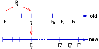
The Gillespie approximation. Our analysis is based on an approximation first introduced by Gillespie Gillespie1983 . The key idea is to ignore the change in available fitness values that occurs after a jump of the adaptive walk, which implies that the entire adaptive process proceeds in a single, fixed neighborhood (Fig. 1). The expected length of the walk is then equal to the first passage time (or absorption time) of the Markov chain defined by the transition probability (1) for a fixed set of fitness values $F_{k}$. For the following discussion it will be convenient to label the fitness values by their rank, such that $F_{1}>F_{2}>...>F_{N}$. The mean absorption time to the final state of maximal fitness $F_{1}$, starting from fitness rank $n$, is then given by Gillespie1983

$$t_{n}=H_{n-1}-\sum_{i=1}^{n-1}\frac{\lambda_{i}}{\lambda_{n}(n-1)}-\sum_{i=1}^{n-1}\sum_{j=i+1}^{n-1}\frac{\lambda_{i}}{\lambda_{j}j(j-1)}$$ (4)

where $H_{k}=\sum_{i=1}^{k}\frac{1}{i}$ is the $k$th harmonic number, and

$$\lambda_{i}=\sum_{k=1}^{i-1}k(F_{k}-F_{k+1})=\sum_{k=1}^{i-1}k\Delta_{k}$$ (5)

with $\lambda_{1}=0$ and fitness gaps $\Delta_{k}=F_{k}-F_{k+1}$. Because fitness only increases during the process, the absorption time is obviously independent of the fitness values $F_{n+1},F_{n+2},...,F_{N}$ above the starting rank.

Within the Gillespie approximation, the adaptive walk length $\ell$ is obtained by averaging the absorption time (4) with respect to the fitness distribution $\rho(F)$. Gillespie observed that the problem simplifies significantly if $\rho(F)$ is assumed to fall into the Gumbel universality class of EVT. Taking the limit $N\to\infty$ at fixed $n$, the $n$ superior fitness values lie in the tail of the distribution, and it is known that the scaled fitness ranks $k\Delta_{k}$ converge to independent, identically distributed exponential random variables deHaan . It then follows by symmetry that the average ratios in (4) are $\langle\frac{\lambda_{i}}{\lambda_{j}}\rangle=\frac{i-1}{j-1}$, and evaluation of the sum yields the simple result Gillespie1983 ; Orr2002 $\langle t_{n}\rangle=\frac{1}{2}(H_{n-1}+1)\approx\frac{1}{2}\ln n+\frac{1}{2}(\gamma+1)$, where $\gamma\approx 0.577215...$ denotes Euler’s constant. Simulations of the full problem show that the mean walk length differs from this approximate result only by an offset in the constant correction term, which is given by $c_{0}\approx\frac{1}{2}(\gamma+1)+0.44$ Orr2002 . A similar calculation for the model with random choice of fitter neighbors yields a mean absorption time of $\langle t_{n}\rangle=H_{n-1}\approx\ln n+\gamma$ Orr2002 , which again differs from the mean walk length of the full model Macken1989 ; Flyvbjerg1992 (quoted above) only by a small shift in the constant term. We will show below that the close agreement between the Gillespie approximation and the full model extends to general fitness distributions, and provide a qualitative explanation for this behavior.

General fitness distributions. We now turn to the approximate evaluation of the absorption time (4) for the other EVT classes. As a representative of the Fréchet class we choose the Pareto distribution $\rho(F)=\mu F^{-(\mu+1)}$, $F\geq 1$, which is a shifted and rescaled version of (2) with $\mu=1/\kappa$. A straightforward calculation shows that the expected value of the $k$th out of $N$ fitness values is given by

$$\langle F_{k}\rangle=\frac{\Gamma(N+1)\Gamma(k-\frac{1}{\mu})}{\Gamma(N+1-\frac{1}{\mu})\Gamma(k)}\approx\left(\frac{N}{k}\right)^{\frac{1}{\mu}}$$ (6)

for $N\gg k\gg 1$. To estimate the fitness gap we take the derivative with respect to $k$ Note2 , $\langle\Delta_{k}\rangle\approx-\frac{\partial}{\partial k}\langle F_{k}\rangle\sim N^{\frac{1}{\mu}}k^{-1-\frac{1}{\mu}}$. Approximating the sum in (5) by an integral we then find $\lambda_{i}\sim N^{\frac{1}{\mu}}i^{1-\frac{1}{\mu}}$, and hence $\lambda_{i}/\lambda_{j}\sim(i/j)^{1-\frac{1}{\mu}}$. Inserting this into (4) and replacing sums by integrals we see that the first sum converges to a constant for $n\to\infty$, while the second, double sum diverges logarithmically as $\frac{\mu}{2\mu-1}\ln n$. Thus to leading order we find $\langle t_{n}\rangle\approx\left(1-\frac{\mu}{2\mu-1}\right)\ln n=\frac{\mu-1}{2\mu-1}\ln n$, which is identical to (3) with $\kappa=1/\mu$.

The calculation for the Weibull class of distributions with bounded support is similar. We consider distributions on the unit interval of the form $\rho(F)=(\nu+1)(1-F)^{\nu}$ with $\nu\geq-1$, corresponding to (2) with $\kappa=-\frac{1}{\nu+1}$. The mean of the $k$th out of $N$ values drawn from this distribution is given by $\langle F_{k}\rangle\approx 1-\left(\frac{k}{N}\right)^{\frac{1}{\nu+1}}$ for $N\gg k\gg 1$, and along the same lines of reasoning used previously we find that $\lambda_{i}/\lambda_{j}\sim(i/j)^{\frac{\nu+2}{\nu+1}}$. Again, this implies that the first sum on the right hand side of (4) converges, whereas the second double sum diverges logarithmically, leading finally to $\langle t_{n}\rangle\approx\left(1-\frac{\nu+1}{2\nu+3}\right)\ln n=\frac{\nu+2}{2\nu+3}\ln n$, in agreement with (3). The result $\ell\approx\frac{2}{3}\ln n$ for the uniform distribution ($\nu=0$) was also obtained in Jain2011 .

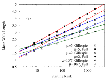
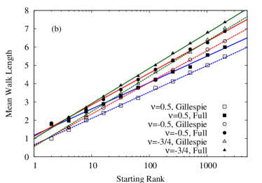
Simulations. Next we compare the prediction (3) to simulations, using both the full adaptive walk model and the simplified Gillespie model in a fixed mutational neighborhood. In the simulations of the full model, we avoided an explicit representation of the genotype space by creating the fitness values encountered during the walk ’on the fly’. This ignores the possibility of the same genotype being encountered more than once during the walk, which is however negligible for large $N$ Flyvbjerg1992 . The total size of the neighborhood was $N=4000$ in all cases, the starting rank was varied from $n=2^{2}=4$ to $n=2^{11}=2048$ in factors of 2, and results were averaged over 1000 independent realizations. As can be seen in Fig. 2, the asymptotic prediction (3) is well satisfied in both kinds of simulations.

Figure 2: (Color online) Simulation results for the full adaptive walk model (full symbols and lines) and the Gillespie approximation (open symbols and dashed lines). Slopes of lines are given by (3) and intercepts have been fitted to the numerical data. (a) Fréchet class with $\mu=\frac{1}{\kappa}=\frac{10}{7}$, 2 and 5. The fitted intercepts are $c_{\kappa}=c_{7/10}=1.60$, $c_{1/2}=1.39$ and $c_{1/5}=1.25$ for the full model and $\tilde{c}_{7/10}=1.27$, $\tilde{c}_{1/2}=1.00$, $\tilde{c}_{1/5}=0.84$ for the Gillespie approximation. (b) Weibull class with $\nu=-(1+\frac{1}{\kappa})=-0.75$, $-0.5$ and $0.5$. Fitted intercepts are $c_{-2/3}=1.18$, $\tilde{c}_{-2/3}=0.66$, $c_{-2}=1.12$, $\tilde{c}_{-2}=0.61$, $c_{-4}=1.00$ and $\tilde{c}_{-4}=0.56$ . In all cases $c_{\kappa}>\tilde{c}_{\kappa}$.

To rationalize the observed close agreement between the Gillespie approximation and the full adaptive walk, we analyze the effect that the two processes involved in a single step of the walk have on the rank of the current genotype (Fig. 1). In the first process, the choice of a fitter neighbor according to the transition probability $P_{ij}$, the rank of the genotype changes by an amount that is proportional to the initial rank; to be specific, the expected new rank $j$ conditioned on the original rank $i$ is given by $\langle j\rangle=\frac{1}{2}\beta i$ for $i\gg 1$ Joyce2008 . The change of rank due to the subsequent change of the mutational neighborhood (which is omitted in the Gillespie approximation) can be deduced from the classic analysis of the number of exceedances Rokyta2006 ; Gumbel1950 , which shows that the expected new rank $j^{\prime}$ conditioned on the old rank $j$ is $j+1$, with a variance of order $j$. Thus for $i,j\gg 1$ the change in rank due to the change in neighborhood is a small perturbation (of relative size $\frac{1}{\sqrt{j}}$) of the change that occurs in the first process, which explains the quantitative accuracy of the Gillespie approximation. The fact that the change of neighborhood on average increases the rank is consistent with the numerical observation that the adaptive walks in the full model are always slightly longer than in the Gillespie approximation (Fig. 2).

Relation to quasispecies models. The quasispecies approach to evolution assumes very large populations, $MU\to\infty$, such that demographic fluctuations are absent and the adaptive process is completely deterministic Jain2007a . In an uncorrelated random fitness landscape the most populated genotype then performs a kind of ‘adaptive flight’, which is essentially constrained to move between local fitness maxima and terminates only when the global fitness maximum is reached Krug2003 ; Jain2005 . In the simple case of a one-dimensional genotype space, the length of such an adaptive flight depends logarithmically on the number of genotypes with a prefactor given precisely by the expression in (3), a behavior that was first observed numerically Krug2003 and subsequently derived analytically in Sire2006 . The formal relation to the adaptive walk problem can be traced back to the fact that the transition probability of the adaptive flight, which describes the rate at which the most populated genotype jumps from one fitness peak to the next, depends linearly on the fitness difference between the two peaks in the same way as the fixation probability (1) Sire2006 . This structure also appears in the analysis of the collision statistics of a one–dimensional gas with quenched random velocities Bena2007 .

Employing a completely different mathematical approach, Sire et al. Sire2006 computed the mean length of the adaptive flights as well as the corresponding variance (see also Bena2007 ). Using their result one finds that the index of dispersion $I$ (defined as the ratio of the variance to the mean) depends on the EVT parameter $\kappa$ according to the simple expression $I=\frac{1+(1-\kappa)^{2}}{(2-\kappa)^{2}}$, which takes its minimal value $I=\frac{1}{2}$ for the Gumbel class ($\kappa=0$) and approaches unity for $\kappa\to-\infty$ as well as for $\kappa\to 1$. This formula reproduces the results obtained in Jain2011 for $\kappa=0$ and $\kappa=-1$, and we have checked numerically that it applies to the full adaptive walks problem for general $\kappa$. Thus, while the walk length has a Poisson distribution in the case of random dynamics Flyvbjerg1992 , in general the fluctuations are sub-Poissonian.

Conclusions. We have analyzed a simple, paradigmatic model for the evolution of populations subject to rare mutations and strong selection, and derived a precise asymptotic relation between the length of adaptive walks and the tail of the underlying fitness distribution. While the predicted asymptotics may be difficult to observe in experiments, the EVT shape parameter $\kappa$ can be estimated experimentally Beisel2007 , and examples with $\kappa=0$ Kassen2006 , $\kappa<0$ Rokyta2008 and $\kappa>0$ Schenk have been identified.

An important restriction of our model is the assumption that fitness values of different genotypes are uncorrelated. Indeed, a recent study comparing the distributions of beneficial fitness effects encountered during the first and second steps of an adaptive walk found strong evidence for fitness correlations between neighboring genotypes Miller2011 . Such correlations are likely to significantly affect the results presented here, and will be addressed in the future.