Scaling of mean first-passage time as efficiency measure of nodes sending information on scale-free Koch networks

Abstract

Random walks on complex networks, especially scale-free networks, have attracted considerable interest in the past few years. A lot of previous work showed that the average receiving time (ART), i.e., the average of mean first-passage time (MFPT) for random walks to a given hub node (node with maximum degree) averaged over all starting points in scale-free small-world networks exhibits a sublinear or linear dependence on network order $N$ (number of nodes), which indicates that hub nodes are very efficient in receiving information if one looks upon the random walker as an information messenger. Thus far, the efficiency of a hub node sending information on scale-free small-world networks has not been addressed yet. In this paper, we study random walks on the class of Koch networks with scale-free behavior and small-world effect. We derive some basic properties for random walks on the Koch network family, based on which we calculate analytically the average sending time (AST) defined as the average of MFPTs from a hub node to all other nodes, excluding the hub itself. The obtained closed-form expression displays that in large networks the AST grows with network order as $N\ln N$, which is larger than the linear scaling of ART to the hub from other nodes. On the other hand, we also address the case with the information sender distributed uniformly among the Koch networks, and derive analytically the global mean first-passage time, namely, the average of MFPTs between all couples of nodes, the leading scaling of which is identical to that of AST. From the obtained results, we present that although hub nodes are more efficient for receiving information than other nodes, they display a qualitatively similar speed for sending information as non-hub nodes. Moreover, we show that that AST from a starting point (sender) to all possible targets is not sensitively affected by the sender’s location. The present findings are helpful for better understanding random walks performed on scale-free small-world networks.

1 Introduction

In recent ten years, as a powerful mathematic tool, as well as a paradigmatic model in the intense research of complex systems, complex networks have attracted a surge of interest from the scientific community AlBa02 ; DoMe02 ; Ne03 ; BoLaMoChHw06 . Most endeavors in the initial few years were devoted to unveil the nontrivial topological properties of real systems AlBa02 ; DoMe02 . A lot of empirical studies unraveled that a large variety of real-life networks display simultaneously small-world effect WaSt98 and scale-free behavior characterized by a power-law degree distribution BaAl99 . These two important discoveries have radically altered our understanding for structural aspects of complex networked systems.

After making substantial progress in characterizing the complexity of real systems, the focus has shifted to dynamical processes defined on them DoGoMe08 , with the aim to uncover the intrinsic relationship between dynamical processes and underlying architecture of complex networks, i.e., unravel how deeply the structural features of networks affect dynamical processes occurring on them. It has been shown that the power-law degree distribution of scale-free networks fundamentally influence almost all dynamical processes taking place on them, such as disease spreading PaVe01 , percolation CaNeStWa00 , games SaPa05 ; SaSaPa08 , synchronization ArDiKuMoZh08 , to name a few.

In addition to above-mentioned dynamical processes, scale-free structure also strongly affects the efficiency for random walks with an immobile trap fixed at a hub node with the highest degree KiCaHaAr08 ; ZhQiZhXiGu09 ; ZhGuXiQiZh09 ; AgBu09 ; TeBeVo09 ; AgBuMa10 . It was surprisingly found that the average receiving time (ART), i.e., the average of mean first-passage time (MFPT) for a random walker to a given target hub node, averaged over all source points in scale-free small-world networks, behaves sublinearly or linearly with the network order (viz., the number of all nodes). Here the MFPT from site $u$ to $v$ is defined as the expected time for a walker starting from $u$ to first reach $v$ Re01 ; NoRi04 . Since the random walker can be looked upon as an information messenger NoRi04 ; ChBa07 , the low ART to the hub node means that as information receivers nodes with large degree are efficient in receiving information. However, any node in a network can also be treated as an information sender. Then, interesting questions are raised naturally: What is the scaling of the average sending time (AST), defined as the average of MFPTs from a hub node to any other node, chosen uniformly in a scale-free network? Is it still as efficient as the case that the hub is regarded as a receiver? Does the location of information sender affect the scaling of AST? Despite the significance of the questions, they still remain unclear limited by the difficulty for determining MFPT from a hub node to some other nodes Bobe05 .

In this paper, we study analytically random walks on the class of Koch networks with scale-free behavior and small-world effect ZhZhXiChLiGu09 ; ZhGaChZhZhGu10 , which is a fundamental process gaining considerable recent attention MeKl04 ; NoRi04a ; SoRebe05 ; BaLo06 ; CoBeTeVoKl07 ; GaSoHaMa07 ; CoTeVoBeKl08 ; BeChKlMeVo10 ; BeGrLeLoVo10 . We first investigate a particular random walk, starting from a hub node with highest degree to send information to all other nodes, exclusive the hub itself. We derive exactly the AST from the hub to another node, averaged over all nodes in the Koch networks. The obtained explicit formula displays that in large networks with $N$ nodes, the AST grows asymptotically with $N$ as $N\ln N$, which in sharp contrast to the linear dependence of the ART from all nodes to the hub ZhZhXiChLiGu09 .

In the second part of this work, based on the connection between random walks and electrical networks, we determine analytically the global mean first-passage time (GMFPT), defined as the average of MFPTs over all node pairs. We present that the GMFPT is also asymptotic to $N\ln N$. Since the GMFPT can be looked upon as the average of ASTs with the sender distributed uniformly among all nodes, we conclude that neither the structure inhomogeneity nor the position of starting points has an essential effect on the scaling of AST in Koch networks. Thus, the $N\ln N$ behavior of AST from a particular sender is a representative property of the Koch networks, which is in comparison with the trapping problem, where the scaling of ART to a trap (information receiver) depends on the location of the trap TeBeVo09 .

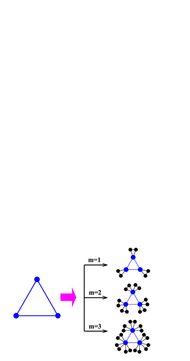
Figure 1: (Color online) Iterative construction method for the Koch networks.

2 Koch networks and their structural properties

The family of Koch networks controlled by a positive integer parameter $m$ are translated from the famous Koch fractals LaVaMeVa87 and can be built in an iterative way ZhZhXiChLiGu09 ; ZhGaChZhZhGu10 . Denote by $K_{m,t}$ the Koch network family after $t$ iterations. Then, the Koch networks can be created in the following way: Initially ($t=0$), $K_{m,0}$ consists of three nodes forming a triangle. For $t\geq 1$, $K_{m,t}$ is obtained from $K_{m,t-1}$ by adding $m$ groups of nodes for each of the three nodes of every existing triangle in $K_{m,t-1}$. Each node group includes two nodes, both of which and their “mother” node are linked to each other constituting a new triangle. In other words, in order to get $K_{m,t}$ from $K_{m,t-1}$, one can substitute a connected cluster on the right-hand side (rhs) of arrow in Fig. 1 for each triangle in $K_{m,t-1}$. Figure 2 illustrates a Koch network for the case of $m=2$ after several iterations.

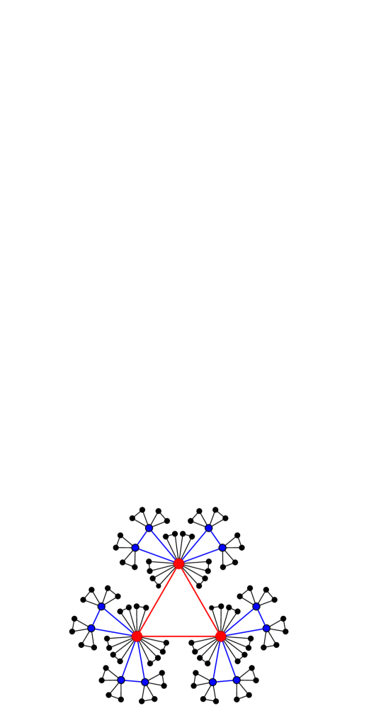
Figure 2: (Color online) A network corresponding to the case of $m=2$.

By construction, we can obtain with ease some quantities that will be very useful for deriving the basic quantity we are concerned in this paper. It is obvious that the number of triangles $L_{\triangle}(t)$ present at iteration $t$ is $L_{\triangle}(t)=(3m+1)^{t}$, and the number of nodes generated at iteration $t$ is $L_{v}(t)=6m\,L_{\triangle}(t-1)=6m\,(3m+1)^{t-1}$. Then, the numbers of edges and nodes in networks $K_{m,t}$ are

$$E_{t}=3\,L_{\triangle}(t)=3(3m+1)^{t}\,$$ (1)

and

$$N_{t}=\sum_{t_{i}=0}^{t}L_{v}(t_{i})=2\,(3m+1)^{t}+1\,,$$ (2)

respectively.

Denote by $k_{i}(t)$ the degree of a node $i$ at iteration $t$ that entered the networks at iteration (step) $t_{i}$ ($t_{i}\geq 0$). Then, $k_{i}(t_{i})=2$. Denote by $L_{\triangle}(i,t)$ the number of triangles passing by node $i$ at step $t$. According to the network generation algorithm, each triangle passing node $i$ at a given step will lead to $m$ new triangles involving $i$ at next time step. Hence, $L_{\triangle}(i,t)=(m+1)\,L_{\triangle}(i,t-1)=(m+1)^{t-t_{i}}$. In addition, the relation $k_{i}(t)=2\,L_{\triangle}(i,t)$ holds. Then $k_{i}(t)=2(m+1)^{t-t_{i}}$ that indicates

$$k_{i}(t)=(m+1)\,k_{i}(t-1).$$ (3)

Note that in $K_{m,t}$ the initial three nodes created at iteration 0 have the highest degree $2(m+1)^{t}$. We call these nodes hub nodes and label by 1 one of the hub nodes, while label the other two hubs by 2 and 3, respectively.

The Koch networks exhibit some classic characteristics of real-life systems ZhZhXiChLiGu09 ; ZhGaChZhZhGu10 . They are scale-free with their degree distribution $P(k)$ following a power-law form $P(k)\sim k^{-\gamma}$, where $\gamma$ is equal to $1+\frac{\ln(3m+1)}{\ln(m+1)}$ belonging to the interval $[2,3]$. They display small-world effect with a small average path length (APL) and a large clustering coefficient. Their APL exhibits a logarithmic scaling with network order $N_{t}$.

3 Basic properties of Random walks on Koch networks

After introducing the Koch networks $K_{m,t}$ and their topological features, we proceed to study standard random walks NoRi04 running on $K_{m,t}$. At each step the walker, located on a given node, moves uniformly to any of its nearest neighbors. Our main aim is to find the AST from one of the three hub nodes (e.g., node 1) to another node averaged over all target nodes except the hub node itself. To achieve this goal, we provide some essential properties for random walks on the Koch networks.

3.1 Evolutionary rule for mean first-passage time

We fist establish the scaling relation governing the evolution of MFPT between an arbitrary pair of two nodes, using the approach based on underlying backward equations Bobe05 ; HaBe87 ; ZhZhZhYiGu09 . Let $F_{ij}(t)$ express the MFPT of the walker in networks $K_{m,t}$, starting from node $i$ to visit node $j$ for the first time. Because of the particular construction the Koch networks, the exact relation governing $F_{ij}(t+1)$ and $F_{ij}(t)$ can be given.

Consider an arbitrary node $i$ in the Koch networks $K_{m,t}$ after $t$ iterations. Equation (3) indicates that upon growth of the networks from generation $t$ to $t+1$, the degree $k_{i}(t)$ of node $i$ grows by $m$ times, i.e., it increases from $k_{i}(t)$ to $(m+1)k_{i}(t)$. Denote by $X$ the MFPT from node $i$ to any of its $k_{i}$ old neighbors belonging to $K_{m,t}$, and denote by $Y$ MFPT for a walker starting from any of the $mk_{i}$ new neighbors of $i$ created at iteration $t+1$ to one of its $k_{i}$ old neighboring nodes previously existing before iteration $t+1$. Then the following simultaneous equations hold:

$$\left\{\begin{array}[]{ccc}X&=&\frac{1}{m+1}+\frac{m}{m+1}(1+Y),\\ Y&=&\frac{1}{2}(1+X)+\frac{1}{2}(1+Y),\end{array}\right.$$ (6)

which result in $X=3m+1$. Thus, when the networks grow from generation $t$ to $t+1$, the MFPT from any node $i$ ($i\in K_{m,t}$) to any node $j$ ($j\in K_{m,t+1}$) increases on average $3m$ times, namely,

$$F_{ij}(t+1)=(3m+1)\,F_{ij}(t)\,.$$ (7)

This scaling is a basic property of random walks on the Koch networks, which is very useful for deriving our main result.

3.2 Scaling relation and expression for average return time

Let $R_{i}(t)$ denote the expected time for a walker in networks $K_{m,t}$ originating from node $i$ to return to the starting point $i$ for the first time, named mean return time (MRT) in the following text. By definition, we have

$$R_{i}(t)=\frac{1}{k_{i}(t)}\sum_{j\in\Omega_{i}^{(t)}}[1+F_{ji}(t)]\,,$$ (8)

where $\Omega_{i}^{(t)}$ is the set of neighbors of node $i$, which belong to $K_{m,t}$.

On the other hand, for $K_{m,t+1}$,

$$R_{i}(t+1)=\frac{m}{m+1}\times 3+\frac{1}{m+1}\frac{1}{k_{i}(t)}\sum_{j\in\Omega_{i}^{(t)}}[1+F_{ji}(t+1)]\,,$$ (9)

which can be elaborated as follows. The first term on the rhs of Eq. (9) describes the process where the walker moves from node $i$ to its new neighbors and back. Since among all $i$’s neighbors belonging to $K_{m,t+1}$, $\frac{m}{m+1}$ of them are new, such a process happens with a probability of $\frac{m}{m+1}$ and takes three time steps. The second term on the rhs of Eq. (9) accounts for the process in which the walker steps from $i$ to one of the old neighbors $j$ previously existing in $K_{m,t}$ and back; this process occurs with the complimentary probability $\frac{1}{m+1}=1-\frac{m}{m+1}$. Using Eqs. (7) and (8) to simplify Eq. (9), we can obtain the following relation

$$R_{i}(t+1)=\frac{3m+1}{m+1}R_{i}(t)\,.$$ (10)

We next determine the MRT for an arbitrary newly born node in $K_{m,t}$ that is generated at iteration $t$. Let $i^{\prime}$ be a new neighbor of an old node $i$ existing in $K_{m,t-1}$, which is created at iteration $t$. Note that when $i^{\prime}$ was generated, another new node $i^{\prime\prime}$ appeared at the same time and is linked to $i$ and $i^{\prime}$. Let $A$ express the MRT of a walker starting off from $i$ in networks $K_{m,t}$ without ever visiting $i^{\prime}$ and $i^{\prime\prime}$. Then we have the following relations

$$R_{i^{\prime}}(t)=\frac{1}{2}[1+F_{ii^{\prime}}(t)]+\frac{1}{2}[1+F_{i^{\prime\prime}i^{\prime}}(t)]\,,$$ (11)

$$F_{i^{\prime\prime}i^{\prime}}(t)=\frac{1}{2}\times 1+\frac{1}{2}[1+F_{ii^{\prime}}(t)]\,,$$ (12)

and

$$F_{ii^{\prime}}(t)=\frac{1}{k_{i}(t)}+\frac{1}{k_{i}(t)}[1+F_{i^{\prime\prime}i^{\prime}}(t)]+\frac{k_{i}(t)-2}{k_{i}(t)}[A+F_{ii^{\prime}}(t)].$$ (13)

The three terms on the rhs of Eq. (13) can be understood based on the following three processes: with probability $\frac{1}{k_{i}(t)}$, the walker gets from node $i$ to $i^{\prime}$ in one time step; with probability $\frac{1}{k_{i}(t)}$, the walker reaches node $i^{\prime\prime}$ in one time step then takes time $F_{i^{\prime\prime}i^{\prime}}(t)$ to visit $i^{\prime}$; and with the remaining probability $\frac{k_{i}(t)-2}{k_{i}(t)}$, the walker selects uniformly a neighbor node except $i^{\prime}$ and $i^{\prime\prime}$ and spends on average time $A$ in returning to $i$ then takes time $F_{ii^{\prime}}(t)$ to arrive at node $i^{\prime}$.

In order to close Eqs. (11) and (13), we write the MRT of node $i$ as:

$$R_{i}(t)=\frac{1}{k_{i}(t)}\times 3+\frac{1}{k_{i}(t)}\times 3+\frac{k_{i}(t)-2}{k_{i}(t)}\times A\,.$$ (14)

The first (second) on the rhs of Eq. (14) describes the process that the walker steps from $i$ to $i^{\prime}$ ($i^{\prime\prime}$) and back, which occurs with probability $\frac{1}{k_{i}(t)}$ and needs three time steps. The explanation of the third term is analogous to that of Eq. (13).

Eliminating the three intermediate quantities $F_{ii^{\prime}}(t)$, $F_{i^{\prime\prime}i^{\prime}}(t)$, and $A$, we have

$$R_{i^{\prime}}(t)=\frac{k_{i}(t)}{2}\,R_{i}(t).$$ (15)

Combining Eqs. (10) and (15) and considering $k_{i}(t)=2(m+1)^{t-t_{i}}$ lead to the following closed-form expression

$$R_{i^{\prime}}(t)=3(3m+1)^{t}.$$ (16)

Note that Eq. (16) can also be obtained from the Kac formula AlFi99 ; SaDoMe08 , which states that the MRT for a node is in fact the inverse probability to find a particle at this node in the final equilibrium state of the random-walk process.

Equation (16) does not depend the degrees of the old nodes, to which the new nodes $i^{\prime}$ is connected, which means that all the simultaneously emerging new nodes have identical MRT. Since all nodes born at the same time step have identical degree, this is obvious from the Kac formula: for any node with degree $k$ in $K_{m,t}$, its MRT is $\frac{2E_{t}}{k}$, which is consistent with Eq. (16) and in turn implies that Eq. (16) is right.

4 Average sending time from a hub node to another node selected uniformly in the Koch networks

In this section, we investigate the AST from a hub node to another node distributed uniformly in the Koch networks. We focus on the case that the starting point is the hub node 1. Notice that, due to the symmetry, the starting position can be also node 2 or node 3, which does not have any influence on the AST. In what follows, we will show that the particular selection of the starting point makes it possible to derive analytically the relevant quantity, i.e., AST from node 1 to all other nodes. Let $T_{i}(t)$ express the MFPT of node $i$ in $K_{m,t}$, which is the expected time for a walker starting from node $1$ to first hit node $i$. The average of MFPT $T_{i}(t)$ over all target nodes in $K_{m,t}$ is AST, presented by $\langle T\rangle_{t}$, the explicit determination of whose solution is a main goal of the following text.

For the sake of convenient description for calculating $\langle T\rangle_{t}$, we use $\Delta_{t}$ to denote the set of nodes in $K_{m,t}$, and use $\bar{\Delta}_{t}$ to present the set of nodes created at generation $t$. Thus, we have $\Delta_{t}=\bar{\Delta}_{t}\cup\Delta_{t-1}$. By definition, the quantity concerned $\langle T\rangle_{t}$ can be defined as

$$\left\langle T\right\rangle_{t}=\frac{1}{{N_{t}}-1}T_{\text{tot}}(t)\,,$$ (17)

where $T_{\text{tot}}(t)$ is the sum of MFPTs for all nodes starting from the hub node 1, i.e.,

$$T_{\text{tot}}(t)=\sum_{i\in\Delta_{t}}T_{i}(t)\,.$$ (18)

Thus, the problem of determining $\langle T\rangle_{t}$ is reduced to finding $T_{\text{tot}}(t)$. Since all nodes in $K_{m,t}$ belong to either $\Delta_{t-1}$ or $\bar{\Delta}_{t}$, $T_{\text{tot}}(t)$ can be written as the sum of the two following terms:

$$T_{\text{tot}}(t)=\sum_{j^{\prime}\in\bar{\Delta}_{t}}T_{j^{\prime}}(t)+\sum_{j\in\Delta_{t-1}}{{T_{j}}(t)}\,.$$ (19)

Using the relation provided by Eq. (7), Eq. (19) can be recast as

$$T_{\text{tot}}(t)=\sum_{j^{\prime}\in\bar{\Delta}_{t}}T_{j^{\prime}}(t)+(3m+1)T_{\text{tot}}(t-1)\,.$$ (20)

Hence, to calculate $T_{\text{tot}}(t)$, one only need to evaluate the first term on the rhs of Eq. (20), which accounts for the sum of the MFPTs from node 1 to all newly generated nodes at step $t$. Since before visiting node $j^{\prime}$ for a walker starting from node $1$, it must first arrive at node $j$ (an old neighbor of $j^{\prime}$) that previously existed at step $t-1$, then $T_{j^{\prime}}(t)$ can be written as:

$$T_{j^{\prime}}(t)=T_{j}(t)+F_{jj^{\prime}}(t)\,.$$ (21)

Next we will show that $F_{jj^{\prime}}(t)$ can be expressed in terms of the quantity $R_{j^{\prime}}(t)$ that has been determined in preceding section. Note that when $j^{\prime}$ was born, it was linked to node $j$ and a simultaneously emerging node $j^{\prime\prime}$ that was also connected to $j$, then we have the following useful relations:

$$R_{j^{\prime}}(t)=\frac{1}{2}[1+F_{jj^{\prime}}(t)]+\frac{1}{2}[1+F_{j^{\prime\prime}j^{\prime}}(t)]\,,$$ (22)

and

$$F_{j^{\prime\prime}j^{\prime}}(t)=\frac{1}{2}+\frac{1}{2}[1+F_{jj^{\prime}}(t)]\,.$$ (23)

Plugging Eq. (23) into Eq. (22) leads to

$$F_{jj^{\prime}}(t)=\frac{4}{3}R_{j^{\prime}}(t)-2\,.$$ (24)

Inserting the obtained result for $F_{jj^{\prime}}(t)$ given in Eq. (24) into Eq. (21), we obtain

$$T_{j^{\prime}}(t)=T_{j}(t)+\frac{4}{3}R_{j^{\prime}}(t)-2\,.$$ (25)

With the result given by Eq. (25), the first term on the rhs of Eq. (20), denoted by ${T}_{\text{tot}}^{(1)}(t)$, can be expressed as

$${T}_{\text{tot}}^{(1)}(t)=\sum_{j^{\prime}\in\bar{\Delta}_{t}}T_{j^{\prime}}(t)=\sum_{j^{\prime}\in\bar{\Delta}_{t}}\left(T_{j}(t)+\frac{4}{3}R_{j^{\prime}}(t)-2\right).$$ (26)

Since for any node $j$ created at step $t_{j}$ that belongs to $\Delta_{t-1}$, there are $L_{\triangle}(j,t-1)=(m+1)^{t-t_{j}-1}$ triangles passing by $j$, each of which will lead to $2m$ new nodes connecting $j$ at step $t$, then using Eqs. (16) and Eq. (26), the sum $T_{\text{tot}}^{(1)}(t)$ can be rewritten as

$$T^{(1)}_{\text{tot}}(t) = \sum_{j\in\Delta_{t-1}}2mL_{\triangle}(j,t-1)T_{j}(t)+$$ (27)

$$({N_{t}}-{N_{t-1}})\left[\frac{4}{3}\times 3{(3m+1)^{t}}-2\right]$$

$$= \sum_{j\in\Delta_{t-1}}2m(m+1)^{t-t_{j}-1}T_{j}(t)+$$

$$({N_{t}}-{N_{t-1}})\left[\frac{4}{3}\times 3{(3m+1)^{t}}-2\right]\,.$$

The second term on the rhs of Eq. (27) is easy to compute. So, we only need to work out the first term on the rhs of Eq. (27), represented by $T_{\text{sum}}(t)$, namely, $T_{\text{sum}}(t)=\sum_{j\in\Delta_{t-1}}2m(m+1)^{t-t_{j}-1}T_{j}(t)$. Evidently, we have the following recursive relation

$$T_{\text{sum}}(t)$$

$$= (3m+1)(m+1)\sum_{j\in\Delta_{t-2}}2m(m+1)^{t-t_{j}-2}T_{j}(t-1)$$

$$+2m(3m+1)\sum_{j\in\bar{\Delta}_{t-1}}T_{j}(t-1)$$

$$= (3m+1)(m+1)T_{\text{sum}}(t-1)+2m(3m+1)T^{(1)}_{\text{tot}}(t-1)\,.$$

On the other hand, Eq. (27) can be rewritten as

$$T^{(1)}_{\text{tot}}(t)=T_{\text{sum}}(t)+({N_{t}}-{N_{t-1}})\left(4{(3m+1)^{t}}-2\right)\,.$$ (29)

Considering the initial conditions $T^{(1)}_{\text{tot}}(1)=96m^{2}+20m$ and $T_{\text{sum}}(1)=24m^{2}+8m$, we can solve recursively the simultaneous equations (4) and (29) to obtain

$$T_{\text{sum}}(t)=8m\left[(3m+1)^{t-1}+3m(2t-1)(3m+1)^{2(t-1)}\right],$$ (30)

and

$$T^{(1)}_{\text{tot}}(t) = 4m(3m+1)^{t-2}\big{[}6(2mt+2m+1)(3m+1)^{t}$$ (31)

$$-3m-1\big{]}.$$

Inserting Eq. (31) into Eq. (20), we can solve Eq. (20) inductively to yield

$$T_{\text{tot}}(t) = \frac{4}{3}{(3m+1)^{t-1}}[(12mt+12m+2){(3m+1)^{t}}$$ (32)

$$-3mt-3m+1].$$

Inserting Eq. (32) into Eq. (17), we obtain the explicit expression for the AST $\left\langle T\right\rangle_{t}$:

$$\left\langle T\right\rangle_{t}=\frac{2}{{3(3m+1)}}[(12mt+12m+2){(3m+1)^{t}}-3mt-3m+1]\,.$$ (33)

We continue to show how to express the key quantity $\langle T\rangle_{t}$ in terms of the network order $N_{t}$, in order to obtain the relation between these two quantities. Recalling Eq. (2), we have $(3m+1)^{t}=(N_{t}-1)/2$ and $t=[\ln(N_{t}-1)-\ln 2]/\ln(3m+1)$. Thus, Eq. (33) can be further expressed as a function of $N_{t}$ as

$$\langle T\rangle_{t} = \frac{{{N_{t}}-1}}{{3(3m+1)}}\left(\frac{{12m[\ln({N_{t}}-1)-\ln 2]}}{{\ln(3m+1)}}+12m+2\right)-$$

$$\frac{2}{{3(3m+1)}}\left(\frac{{3m[\ln({N_{t}}-1)-\ln 2]}}{{\ln(3m+1)}}+3m-1\right).$$

Thus, for large networks,

$${\left\langle T\right\rangle_{t}}\sim\frac{4m}{(3m+1)\ln(3m+1)}{(N_{t}-1)}\ln{(N_{t}-1)}\,,$$ (35)

showing that the AST grows with increasing order $N_{t}$ as $N_{t}\ln N_{t}$. This leading asymptotic $N_{t}\ln N_{t}$ dependence of AST on the network order is in contrast with the linear scaling of receiving efficiency on network order for a receiver located at the same hub node receiving information sent from all other different nodes ZhZhXiChLiGu09 .

It is known that the exponent $\gamma$ of degree distribution for a scale-free network characterizes the inhomogeneity of the network, which often strongly affects the dynamical processes running on the network Ne03 ; BoLaMoChHw06 ; DoGoMe08 . As shown in section 2, the exponent in the Koch networks is $\gamma=1+\frac{\ln(3m+1)}{\ln(m+1)}$, implying that parameter $m$ controls the extent of heterogeneous structure of the Koch networks: the larger the value of $m$, the more heterogeneous the networks. However, as shown in Eq. (35), although for different $m$ the AST of whole family of Koch networks is quantitatively different, it exhibits the same scaling behavior despite the distinct extent of structure inhomogeneity of the networks corresponding to $m$.

5 Global mean first-passage time for the broadcaster uniformly distributed among all nodes

In the previous section, we have presented that the AST from a most connected node to another node, averaged over all possible target points, exhibits a linear dependence with network order by a logarithmic correction. However, for this case, the information sender is placed on a largest node. Then a question arises naturally whether this scaling is representative. Another interesting issue is whether the diffusion speed still follows the same behavior when the sender is located on other nodes. In the following text, we will study the case that the information sender is uniformly distributed among all nodes in the networks, in order to explore how deeply the position of the sender affect the scaling of transportation efficiency.

5.1 Exact solution to global mean first-passage time

In this case, we are concerned in a new quantity called global mean first-passage time (GMFPT), which is the average of mean first-passage times over all pairs of nodes in the networks. Concretely, the GMFPT in $K_{m,t}$, represented by $\langle F\rangle_{t}$, is defined as

$$\langle F\rangle_{t}=\frac{F_{\rm tot}(t)}{N_{t}(N_{t}-1)}=\frac{1}{N_{t}(N_{t}-1)}\sum_{j=1}^{N_{t}}\sum_{\stackrel{{\scriptstyle i=1}}{{i\neq j}}}^{N_{t}}F_{ij}(t)\,,$$ (36)

in which

$$F_{\rm tot}(t)=\sum_{j=1}^{N_{t}}\sum_{\stackrel{{\scriptstyle i=1}}{{i\neq j}}}^{N_{t}}F_{ij}(t)$$ (37)

is the sum of MFPTs between all pairs of nodes. Note that the definition of GMFPT involves a double average: The first one is over all the walkers to a given target (receiver) $j$, the second one is over a uniform distribution of target nodes among all nodes in $K_{m,t}$.

It should be noticed that the above method used for computing $\langle T\rangle_{t}$ is not applicable to $\langle F\rangle_{t}$, so we must resort to an alternative approach. Fortunately, the peculiar construction of the Koch networks and the link ChRaRuSm89 ; Te91 between effective resistance and the MFPTs for random walks allow to calculate analytically GMFPT $\langle T\rangle_{t}$. We view $K_{m,t}$ as resistor networks DoSn84 by considering each edge to be a unit resistor. Let $R_{ij}(t)$ be the effective resistance between two nodes $i$ and $j$ in the electrical networks obtained from $K_{m,t}$. Then, according to the relation between MFPTs and effective resistance ChRaRuSm89 ; Te91 , we have

$$F_{ij}(t)+F_{ji}(t)=2\,E_{t}\,R_{ij}(t)\,.$$ (38)

Therefore, Eq. (37) can be rewritten as

$$T_{\rm tot}(t)=E_{t}\,\sum_{j=1}^{N_{t}}\sum_{\stackrel{{\scriptstyle i=1}}{{i\neq j}}}^{N_{t}}R_{ij}(t)\,.$$ (39)

Thus, if one knows how to determine the effective resistance, then we have a method to find $\langle F\rangle_{t}$. Then, the question of determining $\langle F\rangle_{t}$ is reduced to computing the total resistance $R_{\rm tot}(t)$ between all pairs of nodes in the resistor networks:

$$R_{\rm tot}(t)=\sum_{j=1}^{N_{t}}\sum_{\stackrel{{\scriptstyle i=1}}{{i\neq j}}}^{N_{t}}R_{ij}(t)\,.$$ (40)

According to the structure of the Koch networks, it is obvious that the effective resistance between any two nodes is exactly $\frac{2}{3}$ times the usual shortest-path distance between the corresponding nodes, i.e.,

$$R_{ij}(t)=\frac{2}{3}d_{ij}(t)\,,$$ (41)

where $d_{ij}(t)$ is the shortest distance between nodes $i$ and $j$ in $K_{m,t}$. Equation (41) can be interpreted as follows. By construction, the Koch networks consist of triangles; moreover, no edge lies in more than one triangle. Then, for any couple of nodes $i$ and $j$ in $K_{m,t}$, the shortest path between them is unique. It is easy to see that the effective resistance between two nodes directly connected by an edge in the shortest path of $i$ and $j$ is $\frac{2}{3}$, which is in fact equal to the effective resistance between two nodes of a triangle. And the $R_{ij}(t)$ can be regarded as the sum of effective resistance of $d_{ij}(t)$ conductors in series, each of which has a effective resistance of $\frac{2}{3}$.

Then, to obtain $\langle F\rangle_{t}$, we need only to calculate the total of shortest distances between all node pairs, denoted by $D_{\rm tot}(t)$, namely

$$D_{\rm tot}(t)=\sum_{i\neq j}\sum_{j=1}^{N_{t}}d_{ij}(t)\,.$$ (42)

It is then obvious to have

$$R_{\rm tot}(t)=\frac{2}{3}\,D_{\rm tot}(t)\,.$$ (43)

Hence, all that is left to find $\langle F\rangle_{t}$ is to evaluate $D_{\rm tot}(t)$.

According to our previous result ZhGaChZhZhGu10 , we can easily obtain the closed-form expression for $D_{\rm tot}(t)$:

$$D_{\rm tot}(t)$$

$$= \frac{2(3m+1)^{t-1}}{3}\left[3m+5+(24mt+24m+4)(3m+1)^{t}\right].$$

Combining above-obtained results, we arrive at the explicit solution to $\langle F\rangle_{t}$:

$$\langle F\rangle_{t}$$

$$= \frac{2}{3}\frac{1}{N_{t}(N_{t}-1)}E_{t}\,D_{\rm tot}(t)$$

$$= \frac{2(3m+1)^{t-1}}{6(3m+1)^{t}+3}\left[3m+5+(24mt+24m+4)(3m+1)^{t}\right],$$

which can be expressed in terms of network order $N_{t}$ as

$$\langle F\rangle_{t} = \frac{1}{3(3m+1)}\frac{N_{t}-1}{N_{t}}\Big{[}3m+5+(N_{t}-1)$$

$$\Big{(}\frac{12m\ln(N_{t}-1)-12m\ln 2}{\ln(3m+1)}+12m+2\Big{)}\Big{]}\,.$$

Equation (5.1) uncovers the exact dependence relation of GMFPT on network order $N_{t}$ and parameter $m$. For large systems, i.e., $N_{t}\rightarrow\infty$, we have following expression for the leading term of $\langle T\rangle_{t}$:

$$\langle F\rangle_{t}\sim\frac{4m}{(3m+1)\ln(3m+1)}(N_{t}-1)\ln(N_{t}-1)\,,$$ (47)

which is in consistent with the general result given in TeBeVo09 . Thus, similar to the behavior of AST obtained in the previous section, in the large limit of $t$, the GMFPT grows with network order $N_{t}$ as $N_{t}\ln N_{t}$, which is independent of $m$ and thus shows that the structure heterogeneity of the networks has no substantial impact on the scaling of GMFPT. The sameness for the leading behavior between $\langle T\rangle_{t}$ and $\langle F\rangle_{t}$ implies that the $N_{t}\ln N_{t}$ scaling of $\langle T\rangle_{t}$ from a hub node to all other nodes is a representative feature for information sending in the Koch networks.

The $N_{t}\ln N_{t}$ behavior found for both the AST and GMFPT can be understood from the following heuristic explanations. The couples of nodes farthest apart (between each other and from the hub due to its centrality) provide the leading contribute for the related MFPTs ZhLiMa10 . On the other hand, for the ART related to the trapping problem with the trap fixed on a hub node, since the hub is relatively easy to reach for most nodes, the ART is relatively small and contributes little to GMFPT, see also AgBuMa10 .

Note that if the information sender is positioned at an arbitrary non-hub node in networks $K_{m,t}$. The AST from the sender to all other nodes also follows the scaling $N_{t}\ln N_{t}$. Because in most of this case, the information must be first delivered to a hub node in a time at most proportional to network order $N_{t}$ ZhZhXiChLiGu09 , then the piece of information proceeds to be sent, until it reaches the receiver after an average transmit time $N_{t}\ln N_{t}$ as shown in the previous section. To confirm this, we have computed analytically the AST for the sender located at new neighbor of hub node $1$ created at step $t$, and obtained the same expression as Eqs. (35) and (47).

6 Conclusions

We have studied random walks on the Koch network family, exhibiting synchronously scale-free and small-world behaviors. We first concentrated on a specific case for random walks from a hub node to all other nodes, and obtained explicitly the formula for AST from this most connected node to different target nodes, which varies with network order $N$ as $N\ln N$, larger than the ART from all other nodes to the hub. Then we continued to derive the GMFPT between two arbitrary nodes averaged over all node couples in the Koch networks, which can be regarded as the average of MFPTs from a uniformly-selected starting point to all other nodes in the networks. We presented that in the limit of large network order $N$, the GMFPT also scales approximatively with $N$ as $N\ln N$. This identity of scalings between the AST and GMFPT indicates that the ability (efficiency) of hub nodes sending information is the same as that the average efficiency of all nodes in the Koch networks, showing that the sending efficiency measured by AST is not sensitively influenced by the position of information sender and the structural heterogeneity of the networks. Finally, it should be mentioned that we only studied a particular family of scale-free networks, whether the conclusion also holds for other scale-free networks, even general networks, needs further investigation in the future.

References

- (1) R. Albert and A.-L. Barabási, Rev. Mod. Phys. 74, 47 (2002).
- (2) S. N. Dorogvtsev and J.F.F. Mendes, Adv. Phys. 51, 1079 (2002).
- (3) M. E. J. Newman, SIAM Rev. 45, 167 (2003).
- (4) S. Boccaletti, V. Latora, Y. Moreno, M. Chavezf, and D.-U. Hwanga, Phy. Rep. 424, 175 (2006).
- (5) D.J. Watts and H. Strogatz, Nature (London) 393, 440 (1998).
- (6) A.-L. Barabási and R. Albert, Science 286, 509 (1999).
- (7) S. N. Dorogovtsev, A. V. Goltsev and J. F. F. Mendes, Rev. Mod. Phys. 80, 1275 (2008).
- (8) R. Pastor-Satorras and A. Vespignani, Phys. Rev. Lett. 86, 3200 (2001).
- (9) D. S. Callaway, M. E. J. Newman, S. H. Strogatz, and D. J. Watts, Phys. Rev. Lett. 85, 5468 (2000).
- (10) F. C. Santos and J. M. Pacheco, Phys. Rev. Lett. 95, 098104 (2005).
- (11) F. C. Santos, M. D. Santos, and J. M. Pacheco, Nature (London) 454, 213 (2008).
- (12) A. Arenas, A. Díaz-Guilera, J. Kurths, Y. Moreno, and C. S. Zhou, Phy. Rep. 469, 93 (2008).
- (13) A. Kittas, S. Carmi, S. Havlin, and P. Argyrakis, EPL 84, 40008 (2008).
- (14) Z. Z. Zhang, Y. Qi, S. G. Zhou, W. L. Xie, and J. H. Guan, Phys. Rev. E 79, 021127 (2009).
- (15) Z. Z. Zhang, J. H. Guan, W. L. Xie, Y. Qi, and S. G. Zhou, EPL, 86, 10006 (2009).
- (16) E. Agliari and R. Burioni, Phys. Rev. E 80, 031125 (2009).
- (17) V. Tejedor, O. Bénichou, and R. Voituriez, Phys. Rev. E 80, 065104(R) (2009).
- (18) E. Agliari, R. Burioni, and A. Manzotti, Phys. Rev. E 82, 011118 (2010).
- (19) S. Redner, A Guide to First-Passage Processes (Cambridge University Press, Cambridge, 2001).
- (20) J. D. Noh and H. Rieger, Phys. Rev. Lett. 92, 118701 (2004).
- (21) C. Chennubhotla and I. Bahar, PLoS Comput. Biol. 3, 1716 (2007).
- (22) E. Bollt and D. ben-Avraham, New J. Phys. 7, 26 (2005).
- (23) Z. Z. Zhang, S. G. Zhou, W. L. Xie, L. C. Chen, Y. Lin, and J. H. Guan, Phys. Rev. E 79, 061113 (2009).
- (24) Z. Z. Zhang, S. Y. Gao, L. C. Chen, S. G. Zhou, H. J. Zhang, and J. H. Guan, J. Phys. A 43, 395101 (2010).
- (25) R. Metzler and J. Klafter, J. Phys. A 37, R161 (2004).
- (26) J. D. Noh and H. Rieger, Phys. Rev. E 69, 036111 (2004).
- (27) V. Sood, S. Redner, and D. ben-Avraham, J. Phys. A 38, 109 (2005).
- (28) A. Baronchelli and V. Loreto, Phys. Rev. E 73, 026103 (2006).
- (29) S. Condamin, O. Bénichou, V. Tejedor, R. Voituriez, and J. Klafter, Nature (London) 450, 77 (2007).
- (30) L. K. Gallos, C. Song, S. Havlin, and H. A. Makse, Proc. Natl. Acad. Sci. U.S.A. 104, 7746 (2007).
- (31) S. Condamin, V. Tejedor, R. Voituriez, O. Bénichou and J. Klafter, Proc. Natl. Acad. Sci. U.S.A. 105, 5675 (2008).
- (32) O. Bénichou, C. Chevalier, J. Klafter, B. Mayer, and R. Voituriez, Nat. Chem. 2, 472 (2010).
- (33) O. Bénichou, D. Grebenkov, P. Levitz, C. Loverdo, and R. Voituriez, Phys. Rev. Lett. 105, 150606 (2010).
- (34) A. Lakhtakia, V. K. Varadan, R. Messier, and V. V. Varadan, J. Phys. A 20, 3537 (1987).
- (35) S. Havlin and D. ben-Avraham, Adv. Phys. 36, 695 (1987).
- (36) Z. Z. Zhang, Y. C. Zhang, S. G. Zhou, M. Yin, and J. H. Guan, J. Math. Phys. 50, 033514 (2009).
- (37) D. Aldous and J. Fill, Reversible Markov chains and random walks on graphs, 1999, http://www.stat.berkeley.edu/ aldous/RWG/Chap2.pdf
- (38) A. N. Samukhin, S. N. Dorogovtsev, and J. F. F. Mendes, Phys. Rev. E 77, 036115 (2008).
- (39) A. K. Chandra, P. Raghavan, W. L. Ruzzo, and R. Smolensky, in Proceedings of the 21st Annnual ACM Symposium on the Theory of Computing (ACM Press, New York, 1989), pp. 574-586.
- (40) P. Tetali, J. Theor. Probab. 4, 101 (1991).
- (41) P. G. Doyle and J. L. Snell, Random Walks and Electric Networks (The Mathematical Association of America, Oberlin, OH, 1984); e-print arXiv:math.PR/0001057.
- (42) Z. Z. Zhang, Y. Lin, and Y. J. Ma (unpublished).