Generation and detection of mode-locked spin coherence in (In,Ga)As/GaAs quantum dots by laser pulses of long duration

Abstract

Using optical pulses of variable duration up to 80 ps, we report on spin coherence initialization and its subsequent detection in $n$-type singly-charged quantum dots, subject to a transverse magnetic field, by pump-probe techniques. We demonstrate experimentally and theoretically that the spin coherence generation and readout efficiencies are determined by the ratio of laser pulse duration to spin precession period: An increasing magnetic field suppresses the spin coherence signals for a fixed duration of pump and/or probe pulses, and this suppression occurs for smaller fields the longer the pulse duration is. The reason for suppression is the varying spin orientation due to precession during pulse action.

I Introduction

Research on spin coherence generation, manipulation and detection has become a topical area in semiconductor physics.awschalom_book ; spin_phys A prospective system to study spin coherence is an ensemble of $n$-type quantum dots (QDs). Short optical pulses can induce efficiently long-living spin coherence in such structures which subsequently can be traced by precession about an external magnetic field.PhysRevLett.94.227403 ; greilich06 Due to the combined action of a periodic train of pump pulses and the hyperfine electron-nuclear interaction, a mode-locking of electron spin precession may occur.A.Greilich07212006 ; A.Greilich09282007 ; carter:167403 As a result, an ensemble of about a million QD electron spins is pushed into a regime given by a limited number of precession modes with commensurable frequencies. This may pave a road toward large-scale spintronic applications.

A fundamental question in this regard concerns limitations of spin initialization and detection by optical pulses. In previous studies, pumping and probing of spin excitations were done by short optical pulses with durations no longer than a few picoseconds, much shorter than the period of spin precession about the magnetic field.PhysRevLett.94.227403 ; greilich06 ; A.Greilich07212006 ; A.Greilich09282007 ; carter:167403 The spin initialization is most efficient for laser pulses with area $\Theta=\pi$, requiring high peak powers generated by bulky lasers such as Ti-Sapphire oscillators, for example, pumped by intense continuous wave lasers.

For applications, the use of more compact pulsed solid state lasers is appealing, which typically provide, however, considerably lower output power levels. To reach a pulse area of $\pi$ then, the pulses must have much longer duration. On the other hand, such pulses can also have a much smaller spectral width, so that a less inhomogeneous QD distribution is excited. But the condition that these pulses are much shorter than the precession period is not necessarily fulfilled then, potentially affecting the spin coherence. Usage of lasers with reduced peak powers may be also beneficial in other respects, for example the reduced importance of non-linear optical processes such as two- or multi-photon absorption, which may serve as potential sources of spin decoherence.

Here we address this problem by reporting on mode-locked spin coherence initialization and detection in $n$-type singly-charged QDs, using pump and probe pulses with durations up to 80 ps. We demonstrate experimentally, that the efficiency of initialization and detection depends strongly on the ratio of laser pulse duration to spin precession period. The experimental data are in good agreement with predictions based on a microscopic model.

The paper is organized as follows: In Sec. II the optical techniques are described and the experimental results are presented in Sec. III. Sec. IV provides the theoretical background, and the comparison between experiment and theory is discussed in Sec. V.

II Sample and experiment

We study the spin coherence in an (In,Ga)As/GaAs self-assembled QD ensemble, grown by molecular-beam epitaxy. The sample contains $20$ layers of (In,Ga)As dots, separated by $60$ nm GaAs barriers. The QD density in each layer is about $10^{10}$ dots/cm². $\delta$-sheets of Si donors are positioned $20$ nm below each QD layer with a dopant density roughly equal to the dot density to achieve an average occupation of one resident electron per QD. The sample was thermally annealed at a temperature of $945$ ^∘C for $30$ s. It is mounted in a superconducting split-coil magnet cryostat which allows application of magnetic fields $B$ up to $6$ T. The sample is cooled down to $T=6$ K by helium contact gas. At this temperature, the ground state photoluminescence maximum is at $1.398$ eV. For monitoring the spin precession, an external magnetic field is applied perpendicular to the light propagation direction (Voigt geometry).

The spin precession is traced by time-resolved pump-probe techniques. A Ti:Sapphire laser emits pulses at a repetition rate of $75.75$ MHz, corresponding to a repetition period $T_{R}=13.2$ ns. The range of pulse durations that can be covered with this laser extends from less than 100 fs up to 80 ps. In all cases the precise pulse duration depends on the laser adjustment with variations on the order of 10%. In the case of sub-ps pulses this is not relevant for the physics described below, but for the few 10 ps pulses this leads to slight variations of the measured spin coherence signal, without affecting the general conclusions. We also note, that the spectral width of the pulses decreases inversely with the pulse duration increase, but the pulses are not Fourier-limited for pulse durations exceeding 2 ps.

The laser beam is split into a pump beam and a probe beam, both having the same photon energies resonant to the ground state photoluminescence peak so that they excite the singlet trion transition. Spin polarization of resident electrons and electron-hole complexes is induced by the pump beam, which is modulated by a photoelastic modulator, varying between left- and right-handed circular polarization at a frequency of $50$ kHz. The intensity of the pump is about $5$ times higher than that of the linearly polarized probe beam. Independent of the pump pulse duration the laser output power was adjusted in order to obtain maximal signal amplitude, which is achieved by a pump pulse area of about $\Theta=\pi$.

After transmission through the sample the probe beam is split into two orthogonal polarizations, whose intensities are detected by a balanced photodiode bridge. Depending on the $z$-component of the spin polarization (where $z$ is the light propagation direction) the plane of linear polarization of the probe beam is rotated due to the Faraday rotation (FR) effect which leads to a variation of the intensities of the two split beams. By polarizing the two beams appropriately, either Faraday rotation or ellipticity is measured.glazov2010a The time delay between pump and probe pulses is tuned by a mechanical delay line up to $13$ ns with a precision of about $20$ fs.

This setup is used as long as resonant pump and probe pulses of the same duration are applied. When varying these durations relative to each other, the setup is modified. One laser is then used as pump (probe) only, while a second laser is used as probe (pump). The duration of the pulses emitted from this second laser is fixed at 2 ps. Both lasers are synchronized with an accuracy of about 100 fs by using one of them as master laser for the second laser, whose pulse repetition rate is adjusted accordingly. The photon energies of the pump and probe pulses are kept in resonance with an accuracy of $0.1$ meV.

III Experimental results

Figure 1 shows time resolved Faraday rotation signals, where the durations of pump and probe pulses are equal, $\tau_{\rm pump}=\tau_{\rm probe}$. Different panels correspond to different pulse durations of 2, 10, 30, and 80 ps. In each case different magnetic field strengths $B$ are applied.

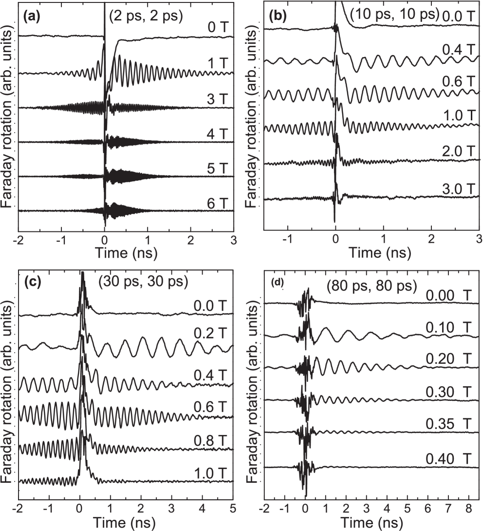
Figure 1: Faraday rotation signals measured as function of time delay between pump and probe at different magnetic fields. The equal pump and probe pulse durations were $\tau_{\rm pump}=\tau_{\rm probe}=2$ ps (a), $10$ ps (b), $30$ ps (c), and 80 ps (d), as indicated by the numbers in brackets giving $(\tau_{\rm pump},\tau_{\rm probe})$. The noise around zero delay comes from scattered laser light, as seen particularly well for the long duration pulses.

For $2$ ps pulses strong Faraday rotation signals appear up to the highest applicable magnetic fields, so that in all cases also mode-locked spin coherence can be generated and detected, in agreement with previous reports.A.Greilich07212006 A prerequisite outlined in these studies is that the pump pulse duration is much shorter than the period of spin precession, given by $T_{e}=2\pi\hbar/(g_{e}\mu_{B}B)$, where $\hbar$ is the Planck constant and $\mu_{B}$ is the Bohr magneton. $g_{e}$ is the average electron $g$ factor of the optically excited QD electron spin ensemble. For our QDs with a $g$ factor of -0.56 at the ground state photoluminescence maximum we obtain $T_{e}$ [ps] $=127/B$[T], which gives 21 ps at $B$=6 T, still an order of magnitude longer than the pulse duration. Therefore the Larmor precession is of negligible influence for the processes of both spin coherence generation and measurement as pump and probe do not average over distinctly varying spin orientations during precession.

We have performed also experiments for pulse durations below 1 ps, and the appearance of the Faraday rotation traces (not shown) for magnetic fields up to 6 T is similar to the one for 2 ps pulses, so that generation and detection of spin coherence work efficiently also in these cases. Our setup permits us, however, also to increase the laser pulse duration to being comparable or even longer than the spin precession period. For this long pulse case the question arises to what extent the spin coherence can still be accessed.

Faraday rotation traces for $10$ ps pulses are shown in Fig. 1(b). The curves recorded for low magnetic fields show strong spin precession signal, but beyond 1 T the signal strength gets continuously weaker. Above about 3 T spin precession can no longer be resolved. As a characteristic quantity for this transition we use the product of Larmor precession frequency, $\Omega_{\rm L}=2\pi/T_{e}$, times the pump pulse duration: $\Omega_{\rm L}\tau_{\rm pump}$. The field strength of 3 T corresponds to a value of 1.5 for this product. This means that during the pump pulse the spins perform about a quarter of a full revolution about the magnetic field. The characteristic value of 1.5 for this product is also found when the pulse duration is extended further. For example, for 30 ps pulses in Fig. 1(c) strong spin coherent signal can be observed up to 0.6 T, beyond the FR signal drops strongly, so that above 1 T the signal strength reaches the noise level. The 1 T field corresponds again to a product of 1.5, as confirmed for pump pulses of 80 ps where the spin coherent signal appears up to 0.4 T only, while for higher fields it cannot be observed anymore.

Note, however, that the magnetic field dependence of the Faraday rotation signal amplitude is quite complicated, because it typically shows a non-monotonous variation with $B$, as can be seen, for example, for the (30 ps, 30 ps) configuration in Fig. 1(c). After being strong at low fields, it drops around 0.4 T, gets stronger again around 0.6 T, and finally vanishes at higher magnetic fields. The origin for this variation is not fully clear yet, as several effects may become relevant such as the variation of the number of mode-locked modes with increasing field, which is particularly relevant at low fields, where only a few precession modes are synchronized. In addition, the nuclear-induced electron spin precession frequency focusing effects involved in the mode locking may vary with field strength.A.Greilich09282007 Independent of that, the disappearance of signal at a characteristic field where $\Omega_{\rm L}\tau_{\rm pump}\sim 1.5$ is valid for all pulse durations.

In a nutshell, spin polarization can be excited and detected by pulses with widely varying durations up to 80 ps. The mode-locking of electron spin coherence is pronounced for any $\tau_{\rm pump}=\tau_{\rm probe}$ as evidenced by the strong signal at negative delays. The efficiency of spin coherence generation depends, however, critically on the parameter $\Omega_{\rm L}\tau_{\rm pump}$. The product $\Omega_{\rm L}\tau_{\rm pump}$ has to be smaller than about 1.5, for higher values spin coherence initialization and measurement do not work anymore. For completeness we note that corresponding ellipticity traces look qualitatively similar to the Faraday rotation traces, even though there are quantitative differences concerning signal amplitudes and in particular the ratio of signals before and after pump pulse application.glazov2010a

In all cases dephasing of the signal is seen on time scales of a few nanoseconds. There are two reasons for this dephasing: the excitation of an inhomogeneous spin ensemble with varying $g$ factors and therefore also varying precession frequencies and the spin precession about the randomly oriented nuclear magnetic field. The latter is important mostly at low magnetic fields, while the $g$ factor inhomogeneity becomes dominant for fields exceeding by far the nuclear field of about 10 mT.Auer

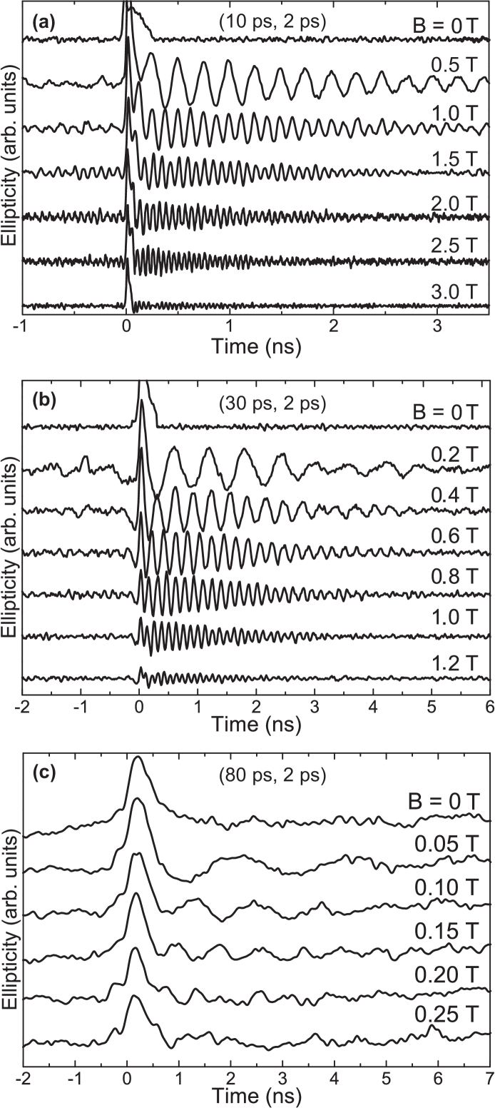
Figure 2: (a) Ellipticity signals recorded with a probe pulse duration of 2 ps, with the pump pulse duration increased to 10 ps in panel (a), 30 ps in panel (b) and 80 ps in panel (c) at different magnetic field strengths. The numbers in brackets give the pump and probe durations $(\tau_{\rm pump},\tau_{\rm probe})$.

In the measurements presented so far, we use pump and probe pulses of the same duration. For the long pulses this means that considerable spin precession of the involved carriers, either resident or photoexcited, occurs during pulse application. This concerns both the initialization of coherence and also its measurement. Ideally these two processes should be separated from one another, which requires independent variation of pump and probe pulse durations relative to each other $(\tau_{\rm pump}\neq\tau_{\rm probe})$.

To that end, we first make experiments, in which the pump pulse duration is varied, while the probe pulse duration is kept constant at 2 ps. From above we know that this pulse duration is short enough that the spin orientation can be considered as frozen. The results are shown in Fig. 2. Figure 2(a) shows the magnetic field series of ellipticity traces for 10 ps pump pulses. Note that traces measured in Faraday rotation show a similar variation with magnetic field, but the signal strength is weaker, as seen from the enhanced noise in the signals. As soon as $\Omega_{\rm L}\tau_{\rm pump}$ passes a certain threshold with increasing $B$, the coherent signal drops considerably, indicating that spin initialization does not work anymore.

When determining the threshold magnetic field, care needs to exercised. On the one hand, due to the longer pump pulse, having correspondingly a reduced spectral width, a smaller number of spins becomes initialized. As a result, a smaller number of mode-locked spin precession modes are involved. One the other hand, the probe still collects signals from a large, partially disordered ensemble. Therefore the signals become overall weaker with increasing pump duration as compared to the short pulse excitation in Fig. 1.

Despite of the weak signal, we see that at 3 T, which was the threshold field for the (10 ps, 10 ps) configuration, the signal gets weak, but can still be observed in Fig. 2(a). This indicates that the threshold field may be slightly higher than in the case of equal pulse duration, and that not only the pumping is influential for the signal, but also the probing. But the difference is small as the spin initialization is hampered when the laser pulse duration exceeds a quarter of revolution during precession. Note also that the dependence of the ellipticity signal amplitude on magnetic field is smooth and shows no strong nonmonotonic variations with $B$ as observed in Fig. 1. Below we will show that this dependence can be explained accounting for the finite pulse duration.

These findings are corroborated when shifting to 30 ps pump pulses [results shown in Fig. 2(b)]. The magnetic field at which the signal drop occurs is about 1.2 T, where the product $\Omega_{\rm L}\tau_{\rm pump}$ is 1.8. This again indicates that the threshold field is slightly larger than in the duration degenerate configuration in Fig. 1. In addition, as was also the case in Fig. 2(a), the drop of the signal amplitude before final disappearance is much more abrupt than in Fig. 1. Hence, the ellipticity signal remains significant up to fields very close to the threshold field and then drops rather fast to zero. That the coherent signals remain significant up to fields close to the threshold, in contrast to the observations in Fig. 1, is another indication for the importance of the probing process.

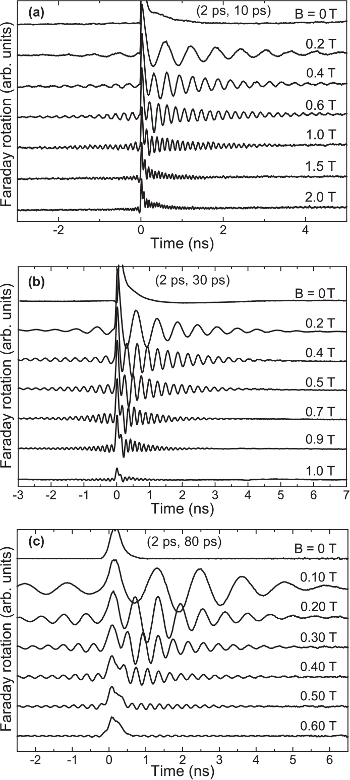
Figure 3: Faraday rotation signals measured for fixed pump pulse duration of 2 ps, but varying probe pulse durations of 10 ps (a), 30 ps (b), and 80 ps (c) at different magnetic fields. The numbers in brackets give the pump and probe durations $(\tau_{\rm pump},\tau_{\rm probe})$.

The overall weak signal for all configurations shown in Fig. 2 becomes particularly pronounced for the 80 ps pump pulse case which is presented in Fig. 2(c). Here faint spin oscillations are seen at positive delays in magnetic fields up to 0.15 T. At higher fields the noise level exceeds the signal amplitude, so that a validation of the threshold criterion is not possible, despite of long accumulation times used in our experiments.

To work out the influence of the pumping, we also test the complementary situation by fixing the pump pulse duration at 2 ps, and changing the probe pulse duration $\tau_{\rm probe}$. By doing so we isolate the effect of the probe on the spin coherence measurement. The probe then has a spectral width always smaller than the pump, so that it tests a spin ensemble smaller than the one addressed the pump, but fully initialized. Typical examples are shown in Fig. 3 for probe pulse durations of 10 ps (a), 30 ps (b) and 80 ps (c). In all cases strong signals are seen, much stronger than in Fig. 2, as seen from the smooth, almost noise-free FR traces, indicating that spin initialization works well. In contrast to the 2 ps probe pulse case where spin coherence can be detected up to 6 T, see Fig. 1(a), we observe here coherent signal only up to 2 T for 10 ps probe, up to 1 T for 30 ps probe, and up to 0.5 T for 80 ps probe. These data suggest that the dependence of the spin signal strength on the parameter $\Omega_{\rm L}\tau_{\rm pump}$ may be transferred also to the probe duration dependence, for which $\Omega_{\rm L}\tau_{\rm probe}$ would be the proper characteristic quantity.

Also here the threshold for $\Omega_{\rm L}\tau_{\rm probe}$ is about 1.5, above which the signal drops fast to zero. Below this threshold the signal amplitude remains considerable as is validated also by Fig. 4, which shows Faraday rotation traces taken for products $\Omega_{\rm L}\tau_{\rm probe}$ equal to 1 and 1.5. For that purpose, different magnetic field strengths are applied for the probe durations of 10, 30, and 80 ps, as seen by the widely varying precession frequencies. When exceeding a product value of unity in every case a considerable drop in Faraday rotation signal strength is observed. The drop occurs, however, rather abruptly when approaching the threshold, similar as in Fig. 2 for ellipticity, but for all probe durations the magnetic field dependencies are smooth, showing no fluctuations..

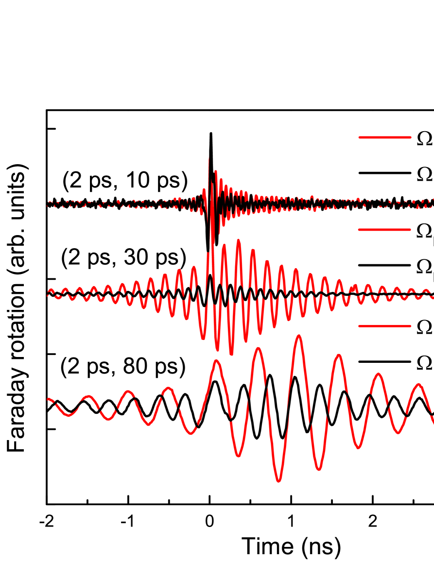
Figure 4: (Color online) Faraday rotation signals measured such that the product $\Omega_{\rm L}\tau_{\rm probe}$ is constant at a value of 1 and 1.5 (except of the 10 ps probe case where the trace for a product value of 1.3 is shown instead of 1.5, because at 1.5 the signal is already very weak). For different probe durations of 10, 30, and 80 ps, the magnetic field strength is adjusted correspondingly, as seen from the varying precession frequencies. The pump pulse duration is fixed at 2 ps. The numbers in brackets give pump and probe durations $(\tau_{\rm pump},\tau_{\rm probe})$. Magnetic fields for the curves are: (i) 2/10 ps: $B=2$ T for $\Omega_{\rm L}\tau_{\rm probe}=1$ and 2.5 T for $\Omega_{\rm L}\tau_{\rm probe}=1.3$, (ii) 2/30 ps: 0.7 T for $\Omega_{\rm L}\tau_{\rm probe}=1.1$ and 1 T for $\Omega_{\rm L}\tau_{\rm probe}=1.5$, (iii) 2/80 ps: 0.25 T for $\Omega_{\rm L}\tau_{\rm probe}=1$ and 0.4 T for $\Omega_{\rm L}\tau_{\rm probe}=1.6$.

All together, we find that the efficiency of spin initialization (measurement) depends sensitively on the pump (probe) duration. The effects of the duration increase for pump and probe have a rather symmetrical impact on the measured signal of spin coherence.

IV Theoretical Model

From the results described so far we find a strong dependence of the spin coherence signal on both pump and probe pulse duration. Therefore a model description of such measurements needs to take into account generation and detection of spin coherence by finite duration pulses. The allowance is made also for the detuning between pump/probe pulse energies and the trion resonance in an individual QD.

IV.1 Basic theory

We consider $n$-type singly-charged QDs pumped and probed by optical pulses propagating along the sample growth axis $z$. We assume that the optical frequencies of pump, $\omega_{\rm pump}$, and probe, $\omega_{\rm probe}$ pulses are close to the one of the singlet $X^{-}$ trion resonance with transition frequency $\omega_{0}$. The QD is subject to a magnetic field which is assumed to be applied along the $x$ axis in the dot plane. The magnetic field induces spin splittings of the electron and trion states. The trion splitting is neglected hereafter because the in-plane heavy-hole $g$ factor is small as compared with the electron $g$ factor. Mar99

We take into account the finite durations of pump ($\tau_{\rm pump}$) and probe ($\tau_{\rm probe}$) pulses, in contrast to Refs. shabaev:201305, ; economou:205415, ; yugova09, where these pulses were considered as negligibly short. In particular, we assume that the pulse duration can be comparable or even longer than the electron spin precession period in magnetic field, $T_{e}$. It is supposed, however, that the pulses are short as compared with the relaxation times in the system $\tau_{\rm pump},\tau_{\rm probe}\ll\tau_{T},\tau_{QD}$ where $\tau_{T}$ is the spin relaxation time of the hole in trion and $\tau_{QD}$ is the trion lifetime in a quantum dot. While the first one is at least in the 100 ns range at $T<$ 10 K, Ref.[hsk ], the trion lifetime is 500 ps, as determined from time-resolved photoluminescence. Therefore, the description of pumping and probing can be carried out using the Schrödinger equation without introducing a spin density matrix.

IV.2 Generation of electron spin coherence

We describe the QD state by a four component wave function $\Psi=[\psi_{1/2},\psi_{-1/2},\psi_{3/2},\psi_{-3/2}]$ where the subscripts $\pm 1/2$ refer to the electron states and the subscripts $\pm 3/2$ refer to the heavy-hole trion states. For a $\sigma^{+}$ polarized pump pulse these components obey the following equations

$$\mathrm{i}\hbar\dot{\psi}_{1/2}=V_{+}^{*}(t)\psi_{3/2}+\frac{\hbar\Omega_{\rm L}}{2}\psi_{-1/2},$$ (1a)

$$\mathrm{i}\hbar\dot{\psi}_{-1/2}=\frac{\hbar\Omega_{\rm L}}{2}\psi_{1/2},$$ (1b)

$$\mathrm{i}\hbar\dot{\psi}_{3/2}=\hbar\omega_{0}\psi_{3/2}+V_{+}(t)\psi_{1/2},$$ (1c)

where $V_{+}(t)=e^{-\mathrm{i}\omega_{\rm pump}t}f_{\rm pump}(t)/\hbar$, with $f_{\rm pump}(t)$ being the smooth envelope of the pump electric field, is the time-dependent matrix element describing the interaction of a $\sigma^{+}$ polarized photon with a QD. This matrix element is proportional to the electric field of the pump pulse and the transition dipole matrix element.yugova09 In the following $f_{\rm pump}(t)$ is assumed to be an even function of time with the maximum at $t=0$. This time moment coincides with the pump pulse arrival. Accounting for the Zeeman splitting in Eqs. (1) is a major difference between the present approach and previous treatments.shabaev:201305 ; economou:205415 ; yugova09 Note, that spin pumping of a free, two-dimensional gas by pulses long as compared with the spin precession period was considered in Ref. averkiev08, .

Without optical pumping, $V_{+}(t)\equiv 0$, the spin system (1) precesses coherently about the in-plane magnetic field. It is convenient to introduce the electron spin state combinations

$$\psi_{x}=\frac{1}{\sqrt{2}}(\psi_{1/2}+\psi_{-1/2}),\quad\psi_{\bar{x}}=\frac{1}{\sqrt{2}}(\psi_{1/2}-\psi_{-1/2}),$$ (2)

that correspond to the eigenstates in magnetic field $\bm{B}\parallel x$ and evolve in time as

$$\psi_{x}(t)=\tilde{\psi}_{x}\ {\exp{({-}\mathrm{i}\Omega_{\rm L}t/2)}},\quad\psi_{\bar{x}}(t)=\tilde{\psi}_{\bar{x}}\ {\exp{(\mathrm{i}\Omega_{\rm L}t/2)}},$$ (3)

where $\tilde{\psi}_{x}$, $\tilde{\psi}_{\bar{x}}$ are constants determined by the initial conditions. With optical pumping, $V_{+}(t)\neq 0$, and $\tilde{\psi}_{x}$, $\tilde{\psi}_{\bar{x}}$ become time-dependent.ll3_eng

In order to describe the pump action on the electron spin we have to establish a link between the spin components before and after pump pulse arrival. The change of spin with time results from two effects: the Larmor precession about the magnetic field and the effect of the pump pulse. The Larmor precession of the electron spin during time $T$ can be described by a linear operator $\mathcal{R}_{\Omega}(T)$.merkulov02 It is convenient to treat the spin precession separately from the optical pulse and connect the rotated electron spin vector $\bm{S}^{-}=\mathcal{R}_{\Omega}(T_{0})\bm{S}(-T_{0})$ with the electron spin vector $\bm{S}^{+}=\mathcal{R}_{\Omega}^{-1}(T_{0})\bm{S}(T_{0})$, where $T_{0}$ exceeds by far the pulse duration so that on the time scale of $T_{0}$ the pulse action can be neglected. On the quantum-mechanical level this operation is equivalent to the unitary transformation Eq. (3). Hence the components of the spin vector $\bm{S}^{\pm}$ are given by:

$$S_{x}^{\pm} = \frac{1}{2}\left[|\tilde{\psi}_{x}(\pm\infty)|^{2}-|\tilde{\psi}_{\bar{x}}(\pm\infty)|^{2}\right],$$

$$S_{y}^{\pm} = -\mathop{\rm Im}\{\tilde{\psi}_{x}(\pm\infty)\tilde{\psi}^{*}_{\bar{x}}(\pm\infty)\},$$ (4)

$$S_{z}^{\pm} = \mathop{\rm Re}\{\tilde{\psi}_{x}(\pm\infty)\tilde{\psi}^{*}_{\bar{x}}(\pm\infty)\}.$$

One can show that in the limit of low pump power (see Appendix A for details)

$$S_{z}^{+}=-\frac{1}{2}\mathop{\rm Re}G(\Lambda,\Omega_{\rm L})+\mathop{\rm Re}{\left[1-\frac{1}{2}G\left(\Lambda+\frac{\Omega_{\rm L}}{2},0\right)-\frac{1}{2}G\left(\Lambda-\frac{\Omega_{\rm L}}{2},0\right)\right]}S_{z}^{-}+\\ \frac{1}{2}\mathop{\rm Im}{\left[G\left(\Lambda+\frac{\Omega_{\rm L}}{2},0\right)+G\left(\Lambda-\frac{\Omega_{\rm L}}{2},0\right)\right]}S_{y}^{-},$$ (5a)

$$S_{x}^{+}=-\frac{1}{4}\mathop{\rm Re}{\left[G\left(\Lambda+\frac{\Omega_{\rm L}}{2},0\right)-G\left(\Lambda-\frac{\Omega_{\rm L}}{2},0\right)\right]}+\mathop{\rm Re}{\left[1-\frac{1}{2}G\left(\Lambda+\frac{\Omega_{\rm L}}{2},0\right)-\frac{1}{2}G\left(\Lambda-\frac{\Omega_{\rm L}}{2},0\right)\right]}S_{x}^{-}-\\ \mathop{\rm Im}{G(\Lambda,\Omega_{\rm L})}S_{y}^{-},$$ (5b)

$$S_{y}^{+}=\mathop{\rm Re}{\left[1-\frac{1}{2}G\left(\Lambda+\frac{\Omega_{\rm L}}{2},0\right)-\frac{1}{2}G\left(\Lambda-\frac{\Omega_{\rm L}}{2},0\right)\right]}S_{y}^{-}+\mathop{\rm Im}{G(\Lambda,\Omega_{\rm L})}S_{x}^{-}-\\ \frac{1}{2}\mathop{\rm Im}{\left[G\left(\Lambda+\frac{\Omega_{\rm L}}{2},0\right)+G\left(\Lambda-\frac{\Omega_{\rm L}}{2},0\right)\right]}S_{z}^{-}.$$ (5c)

where $\Lambda=\omega_{\rm pump}-\omega_{0}$ is the energy detuning between pump pulse and trion resonance. Here

$$G_{\rm pump}(\Lambda,\Omega)=\int_{-\infty}^{\infty}\mathrm{d}tf_{\rm pump}(t)\int_{-\infty}^{t}\mathrm{d}t^{\prime}f_{\rm pump}(t^{\prime})\mathrm{\ }e^{\mathrm{i}\Lambda(t-t^{\prime})}\cos{\left[\frac{\Omega}{2}(t+t^{\prime})\right]}.$$ (6)

The function $G_{\rm pump}(\Lambda,\Omega)$ can be found analytically for Fourier-limited pulses, such as in the case of an exponential pulse, $f_{\rm P}(t)=f_{0}\mathrm{e}^{-|t|/\tau_{\rm pump}}$, where $f_{0}$ is the pump pulse amplitude that is related to its area, $\Theta=2\int\limits_{-\infty}^{\infty}f_{\rm pump}(t)\mathrm{d}t$, by $f_{0}=\Theta/(4\tau_{\rm pump})$. Then one can show that

$$G_{\rm pump}(\Lambda,\Omega)=\frac{\Theta^{2}(2+\mathrm{i}\Lambda\tau_{\rm pump})}{[4+(\Omega\tau_{\rm pump})^{2}][4-8\mathrm{i}\Lambda\tau_{\rm pump}-4(\Lambda\tau_{\rm pump})^{2}+(\Omega\tau_{\rm pump})^{2}]}.$$ (7)

For $\Omega\tau_{\rm pump}=0$, Eq. (7) is equivalent to Eq. (61) of Ref. yugova09, .

Although the Eqs. (5) are quite bulky, they allow one to identify all essential physics features caused by the pump pulse application. First of all, circularly polarized pump pulses cause electron spin orientation along the $z$ axis

$$S_{z}^{+}=-\mathop{\rm Re}{G(\Lambda,\Omega_{\rm L})/2}.$$ (8)

In absence of a magnetic field and for resonant pulse $S_{z}^{+}=-\Theta^{2}/16$. This is equivalent to the regular spin initialization protocol based on very short pump pulses.shabaev:201305 ; greilich06 Due to the Zeeman splitting the spin can acquire some degree of orientation along the $x$ axis due to unequal transition rates out of the magnetic field split sublevels, see first term in Eq. (5b)

$$S_{x}^{+}=-\frac{1}{4}\mathop{\rm Re}{\left[G\left(\Lambda+\frac{\Omega_{\rm L}}{2},0\right)-G\left(\Lambda-\frac{\Omega_{\rm L}}{2},0\right)\right]}.$$ (9)

This effect arises from detuning of the pump pulse from the center of the Zeeman-split doublet, as discussed in more detail below. In addition, the spin is rotated due to the pump pulse action, in the $(xy)$ plane similar to the case of negligible Zeeman splittingeconomou:205415 ; yugova09 ; phelps:237402 and in the $(yz)$ plane due to the combined action of the pump pulse and the spin splitting.

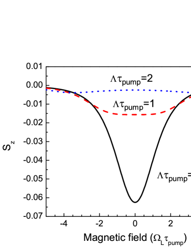
Figure 5: (Color online) Electron spin $z$ component generated by a single pump pulse as a function of reduced magnetic field $\Omega_{\rm L}\tau_{\rm pump}$. The three curves correspond to different detunings between the pump and trion resonance $\Lambda\tau_{\rm pump}=0$ (black/solid), $\Lambda\tau_{\rm pump}=1$ (red/dashed), and $\Lambda\tau_{\rm pump}=2$ (blue/dotted). Pulse area $\Theta=1$.

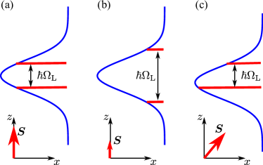
Figure 6: Schematic illustration of electron spin initialization. Red lines indicate Zeeman-split electron sublevels with splitting $\hbar\Omega_{\rm L}$, the blue curve shows the pump pulse spectral shape. (a) and (b) give the case of a pump pulse in resonance with the center of the Zeeman doublet. (a) $\Omega_{\rm L}\tau_{\rm pump}\ll 1$, both sublevels interact strongly with the optical pulse resulting in efficient spin orientation along the $z$ axis. (b) $\Omega_{\rm L}\tau_{\rm pump}\gg 1$, inefficient spin orientation along the $z$ axis. (c) Case of a detuned pulse resulting in different interaction strengths with the Zeeman-split sublevels. As a result the electron spin acquires non-zero $x$ and $z$ components.

It is worth to note that if the electron spin was initially unpolarized, $\bm{S}^{-}=0$, a circularly polarized pump pulse creates electron spin with two non-zero components, $S_{z}^{+}$ and $S_{x}^{+}$. The appearance of $S_{z}^{+}$ is related to the transfer of photon angular momentum to the electron, with an efficiency that decreases with increasing magnetic field, see Fig. 5. Indeed, with increasing spin splitting the formation of a coherent superposition of the Zeeman split sublevels becomes hindered as schematically illustrated in Figs. 6(a) and 6(b). The contained information can be also translated into the time domain: For a fixed Zeeman splitting, the action of a longer pulse corresponds to applying a spectrally narrower pulse, equivalent to going from (a) to (b), and reducing thereby the spin initialization efficiency.

The microscopic origin of the appearance of the in-plane spin component $S_{x}^{+}$ is shown in Fig. 6(c). Indeed, if the pump pulse is detuned from the “center-of-gravity” of the Zeeman-split doublet, the transition efficiencies from the split levels are different. As a result, the resident carrier acquires some spin polarization parallel or anti-parallel to the magnetic field.

As it was assumed that the trion lifetime, $\tau_{QD}$, exceeds by far the pump duration, the dynamics of the coupled electron and trion spins is described in the standard way, see Ref. yugova09, , Eq. (27), and Ref. zhu07, , Eq. (6). Long living electron spin coherence appears after the trion recombination, and a steady state distribution of the precessing spins develops as result of the applied pump pulses.A.Greilich07212006 ; yugova09

IV.3 Detection of electron spin coherence

The description of spin coherence probing is rather similar to the generation. We assume that the probe is linearly polarized along the $x$-axis, i.e. along the magnetic field direction as in our experiment. In this case, the coupled Schrödinger equations describing the dynamics of electron and trion spins separate into two independent subsystems, corresponding to the optical transitions involving electrons with spin parallel to the $x$ axis and those with spin antiparallel to the $x$ axis.

It can be shown that, similarly to Refs. yugova09, ; glazov2010a, , the spin ellipticity, $\mathcal{E}$, and Faraday rotation, $\mathcal{F}$, signals from an ensemble of QD spins are proportional to the real and imaginary parts of the following quantity:

$$\mathcal{E}(t)+\mathrm{i}\mathcal{F}(t)\propto G_{\rm probe}(\omega_{\rm probe}-\omega_{0},\Omega)S_{z}(t),$$ (10)

where $G_{\rm probe}$ is defined by Eq. (6) after replacing the pump envelope $f_{\rm pump}(t)$ by the probe envelope $f_{\rm probe}(t)$. Here $S_{z}(t)$ is the electron spin $z$ component at the moment of probe pulse action, i.e., at the time where the probe pulse amplitude is maximal. In deriving Eq. (10) we assumed that the pump-probe delay exceeds the trion spin lifetime in the QD, $\tau_{T}\tau_{QD}/(\tau_{T}+\tau_{QD})$, which makes possible to neglect the contribution from the trion spin polarization to the measured signal. Otherwise, an additional contribution to Eq. (10) should be taken into account which is proportional to the hole-in-trion spin polarization yugova09 .

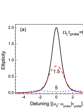
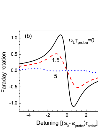
Figure 7: Ellipticity (a) and Faraday rotation (b) signals as function of detuning between the quantum dot resonance and the probe optical frequency. The three curves correspond to different values of magnetic field, $\Omega_{\rm L}\tau_{\rm probe}=0$ (black/solid), $\Omega_{\rm L}\tau_{\rm probe}=1.5$ (red/dashed), and $\Omega_{\rm L}\tau_{\rm probe}=5$ (blue/dotted). The spin $z$ component is the same for all curves. The signals are given in arbitrary units.

Figure 7 shows the dependence of the ellipticty and Faraday rotation signals on the detuning between the trion resonance and the probe optical frequency. Note, that these signals are calculated for a given QD, no averaging over the ensemble is done. The overall behavior is similar to the one known for probing by short pulses, $\Omega_{\rm L}\tau_{\rm probe}\ll 1$ (shown by the black curves in Fig. 7).yugova09 ; carter:167403 The ellipticity is maximal for degenerate probe and trion resonance, while the Faraday rotation has a zero for $\omega_{0}=\omega_{\rm probe}$. With increasing magnetic field the signal strength drops strongly, both in ellipticity and in Faraday rotation for almost all values of the detuning. The maximum of ellipticity transforms into a minimum and a fine structure appears for $\Omega_{\rm L}\tau_{\rm probe}=5$ which corresponds to the probe tuned to the two Zeeman-split sublevels. This fine structure becomes also visible in the Faraday rotation signal. In addition the spectral shape of the signal changes.

The QD ensemble is inhomogeneous, and the pump pulse excites a subensemble of dots with various trion resonance frequencies.glazov2010a Hence, the observed Faraday rotation signal should be averaged over the spin distribution. The result of this averaging depends strongly on the possible asymmetry of the spin distribution as well as on the details of spin coherence excitation and mode-locking. Below, we show that even the simplest model, where the inhomogeneity is ignored and the asymmetry of the quantum dot distribution is modeled as an effective detuning, describes well the experimental findings.

V Comparison of theory and experiment

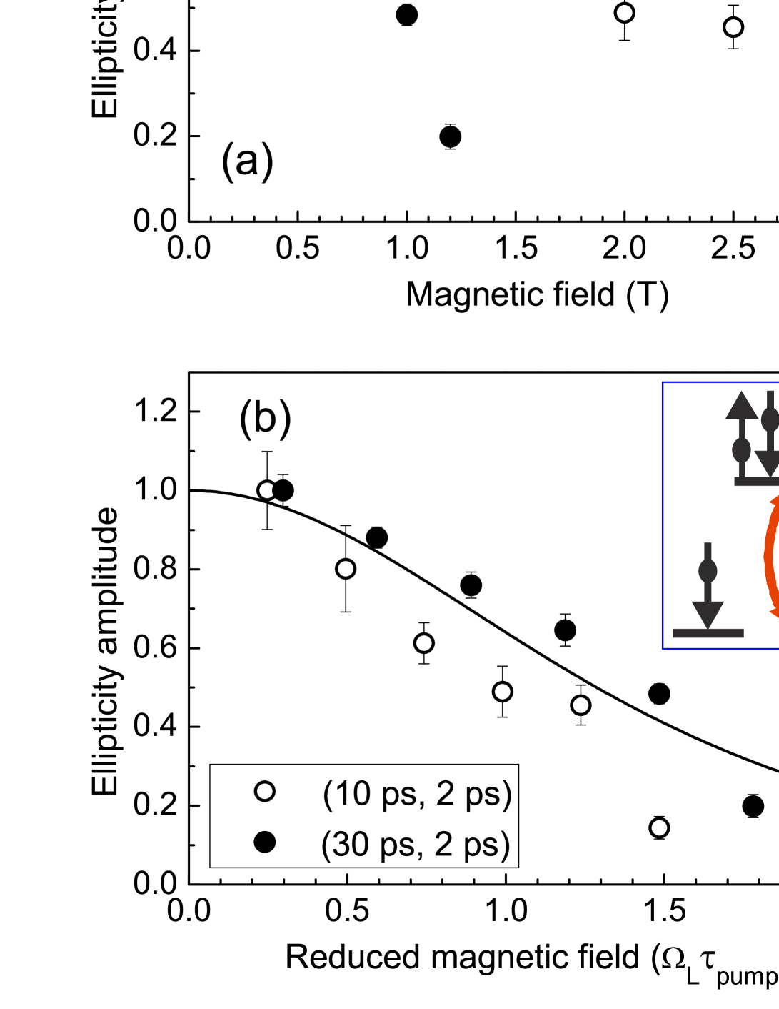
Figure 8: (Color online) Ellipticity amplitude versus magnetic field for pump pulses with a duration of 10 ps and 30 ps, probed by 2 ps pulses. Panel (a) and (b) show the signal amplitude as function of magnetic field and reduced field $\Omega_{\rm L}\tau_{\rm pump}$, respectively. The solid curve in panel (b) is normalized to the $\Omega_{\rm L}\tau_{\rm pump}=0$ dependence of $S_{z}^{+}$, which is the spin component amplitude right after pump pulse arrival, calculated according to Eq. (8). $\omega_{\rm pump}=\omega_{\rm probe}$.

With this general theoretical setting we can compare the calculated magnetic field dependencies of the spin coherence signal with the measured data for different durations of pump pulse and probe pulse. To distinguish between the effects of pump and probe, we focus first on the experiments where one of the pulses was made longer compared to the other pulse with duration fixed at 2 ps. The corresponding experimental data have been shown in Figs. 2 and 3, respectively.

Here we need to comment on the shape of the pump-probe traces. In Ref. glazov2010a, , the ellipticity signal was shown to drop smoothly to zero when moving from zero towards negative or positive delays. For Faraday rotation, however, the signal may rise first before a signal drop due to dephasing is seen, when using resonant pump and probe pulses of the same duration. The Faraday rotation behavior described in Ref. glazov2010a, is observed in Fig. 1, where pump and probe pulses of the same duration were taken from a single laser. The signal rise for short delays is particularly pronounced at 0.2 T in the 30 ps case. When detuning pump and probe spectrally the behavior goes back to the conventional one, like in ellipticity with maximum signal at zero delay. While the traces in Fig. 2 show ellipticity anyway, the traces in Fig. 3 give Faraday rotation signals which, however, have a smooth drop when moving away from time zero, despite of the targeted pump and probe energy resonance. This makes determination of amplitudes quite simple. We attribute this behavior for different pump and probe durations to an effective detuning of the pulses arising from their different spectral widths, where the spectral components outside of the profile of the other laser lead to the effective detuning. In addition the accuracy of putting the pulses from the two lasers in resonance was about 0.1 meV, potentially leading to another small detuning.

From these data we extract the spin coherence signal amplitudes, as measure for the efficiency of either coherence generation or readout. Focusing on the generation process, we have first done this for pump durations of 10 ps and 30 ps, with the probe duration fixed at 2 ps. For determining the amplitudes, the Faraday rotation traces were fitted by exponentially damped harmonics for delay times, when all optically excited exciton complexes have decayed. The amplitudes for different magnetic fields were then normalized by the amplitude for the magnetic field, where the amplitude was maximum.

We also note here, that in contrast to the theoretical modeling (see below) maximum amplitude is reached for finite magnetic fields. We attribute this to the effects of spin precession of the hole in the optically excited trion: the hole $g$ factor $g_{h}$ has been measured to be small, but non-zero ($g_{h}\approx 0.12$) in the structure under study. In low magnetic fields electron spin coherence appears due to the hole spin relaxation only which results in depolarization of the electron left after trion recombination. In higher fields the hole precesses during the trion lifetime which leads in effect to its spin relaxation. As a result, the long-lived electron spin coherence increases in the range of small fields sokolova . In addition, at low external fields nuclear effects can come into play leading to electron depolarization. Therefore we expect a maximum of the electron spin coherence signal at a finite field, $B_{max}$. Experimentally this field lies in the range from 0.1 to 0.2 T.

The magnetic field dependence of the normalized ellipticity amplitudes for 10 ps and 30 ps pump pulses is shown in Fig. 8(a). The amplitude for 30 ps pulses drop smoothly to zero with increasing magnetic field up to slightly more than 1 T. For 10 ps pump pulses the amplitude drop with increasing $B$ does not occur as fast, but takes place over an extended field range up to 3 T. As pointed out, this behavior can be characterized by the reduced magnetic field product $\Omega_{\rm L}\tau_{\rm pump}$, for which we had found that the spin coherence signal basically disappears when the value of 1.5 is exceeded, as confirmed by Fig. 8(b), showing the amplitude data as function of $\Omega_{\rm L}\tau_{\rm pump}$. In this representation the data for the two pump pulse durations basically coincide and converge to zero for $\Omega_{\rm L}\tau_{\rm pump}=1.5$, corroborating the universality of the threshold.

The presence of a threshold, outlined already in the theory subsection, can be qualitatively understood in terms of pulse duration. As schematically shown in the inset of Fig. 8(b), the trion formation is spin selective. For $\sigma^{+}$ polarized light the spin-up electron contributes to the trion and gets depolarized afterwards, while the spin-down electron does not participate in trion formation. These are the electrons whose spin is accumulated due to the train of pump pulses. However, if during the pump pulse action this electron spin component has time to rotate significantly, it also participates in trion formation and becomes depolarized. Thereby the pumping efficiency is diminished.

The solid curve in Fig. 8(b) shows the theoretical result for $S_{z}^{+}$ as a function of reduced magnetic field calculated after Eq. (8). The electron spin $z$ component value at the moment of pump pulse arrival is normalized by its value at $\Omega_{\rm L}\tau_{\rm pump}=0$. The theoretical curve follows rather well the experimental points. The disappearance of spin coherent signal $\Omega_{\rm L}\tau_{\rm pump}=1.5$ can be seen from Fig. 5: compared to the zero value for the product, the initialized spin component is reduced by a factor of about 3 for $\Omega_{\rm L}\tau_{\rm pump}=1$ and it basically has vanished for $\Omega_{\rm L}\tau_{\rm pump}=2$, as the threshold value of 1.5 has been crossed.

The theoretical modeling was done for Fourier-limited pulses, for which we find good agreement with the data, even though the spectral width of the pulses is somewhat larger than expected from their duration. Discrepancies between experiment and theory, also in Fig. 9 might arise, however, from this difference, or from the higher pump excitation power ($\Theta=\pi$) than assumed in theory for the pump.

A similar threshold effect was observed for the influence of the probe pulse, as can be seen from the magnetic field dependence of the Faraday rotation amplitude for different probe durations, while the pump duration was fixed at 2 ps presented in Fig. 9. The probe can reflect the initialization of the spins by the pump only as long as these show a dominant preferential orientation. This is the case for probes shorter than a quarter of revolution during precession. Therefore the drop of the Faraday signal amplitude in Fig. 9(a) occurs at higher magnetic fields when the probe pulses are shorter.

Also for this situation a kind of universal behavior is found in which the absolute magnetic field strength is not decisive but rather the reduced magnetic field strength $\Omega_{\rm L}\tau_{\rm probe}$. Figure 9(b) gives the corresponding dependence of FR signal amplitude. Considering also the experimental accuracy the data for the three different probe pulse durations are close to being identical, indicating a universal behavior on reduced magnetic field. This universal behavior is in accord with the calculations shown by lines in Fig. 9(b). The different calculated curves give different detunings between the probe pulse and trion resonance: $(\omega_{\rm probe}-\omega_{0})\tau_{\rm probe}=0.01$ (solid), $(\omega_{\rm probe}-\omega_{0})\tau_{\rm probe}=0.5$ (dashed) and $(\omega_{\rm probe}-\omega_{0})\tau_{\rm probe}=1$ (dotted), as is the case also in experiment. The difference between these curves is, however, small.

The drop of probed signal amplitude with increasing magnetic field is about the same for Faraday rotation and allipticity as can be seen From Fig. 7. Up to $\Omega_{\rm L}\tau_{\rm probe}=1.5$ the signal amplitude drops by a factor of 2.5 compared with the limit of short pulses. Beyong this threshold the signal drop ocurs rather abruptly. The agreement of the experimental results and theoretical calculations in the simplified model demonstrates that the basic mechanisms of the spin coherence excitation and detection are well understood.

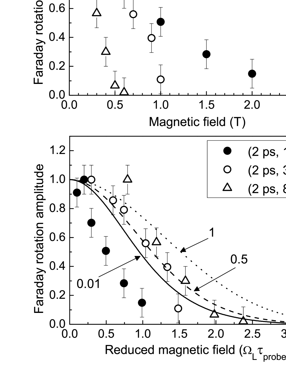
Figure 9: (a) Normalized Faraday rotation amplitudes as functions of magnetic field: squares correspond to $\tau_{\rm probe}=10$ ps, circles to $\tau_{\rm probe}=30$ ps and triangles $\tau_{\rm probe}=80$ ps, while the pump pulse duration was fixed at 2 ps. (b) Normalized Faraday rotation amplitudes versus reduced magnetic field $\Omega_{\rm L}\tau_{\rm pr}$ for the data taken from panel (a). Solid, dashed and dotted curves give calculations using Eq. (10) for different detunings between the probe pulse and the trion resonance $(\omega_{\rm probe}-\omega_{0})\tau_{\rm probe}=0.01$ (solid), $0.5$ (dashed) and $1$ (dotted).

The impact of the finite pump and probe durations is brought together in the experiments with identical pump and probe durations. However, a comparison of the absolute amplitude values is basically impossible, as the corresponding experiments involve different experimental schemes with either a single or two lasers with different focusing on different sample positions in the different measurement runs. Also the magnitude of the pumped and probed spin ensembles varies for the different configurations which involved pulses with either the same or significantly different spectral widths. In addition, we found in Fig. 1 a non-monotonic dependence of the Faraday signal amplitude on magnetic field. Therefore we do not attempt to make a quantitative comparison. Still, qualitatively the picture is quite transparent.

The experiments with either the pump duration or the probe duration varied demonstrate that there is a threshold field above which spin coherence is not found, see Figs. 8(b) and 9(b). In both cases the threshold field is similar for the same pump or probe durations. As the effects of pump and probe enter the spin coherence signal rather ”symmetrically”, a prolongation of both pulses in the duration-degenerate configuration leads to a disappearance of signal amplitude at basically the same field strength. From the calculations we find that the spin coherence drop due to the combined action of a pump and a probe elongation lead sot a signal drop by about an order of magnitude for $\Omega_{\rm L}\tau_{\rm pump}=1.5$ and $\tau_{\rm pump}=\tau_{\rm probe}$. This explains the disappearance of the spin coherent signal at this threshold value.

VI Conclusions

To conclude, we have demonstrated theoretically and experimentally the feasibility to initialize and detect electron spin coherence by long optical pulses with durations up to 80 ps, comparable with the electron spin precession period. The efficiency of electron spin coherence measurement is determined by the ratio of the periods for pulse duration and spin precession and with an increase of the magnetic field the spin signals decrease. The experimental results and theoretical calculations are in good agreement. Based on this demonstration spin initialization by compact pulsed solid state lasers with limited output power becomes feasible in low magnetic fields, to which applications would be limited anyway in applications.

Appendix A Spin pumping by long pulses

The pump pulse effect is conveniently described by an operator $\mathcal{Q}$ which transforms the pair $[\tilde{\psi}_{x}(-\infty)$, $\tilde{\psi}_{\bar{x}}(-\infty)]$ components of the wave function (long before the pulse arrival) into the pair $[\tilde{\psi}_{x}(+\infty)$, $\tilde{\psi}_{\bar{x}}(+\infty)]$ (after pulse arrival):

$$\tilde{\psi}_{x}(+\infty)=\mathcal{Q}_{xx}\tilde{\psi}_{x}(-\infty)+\mathcal{Q}_{x\bar{x}}\tilde{\psi}_{\bar{x}}(-\infty),$$ (11)

$$\tilde{\psi}_{\bar{x}}(+\infty)=\mathcal{Q}_{\bar{x}x}\tilde{\psi}_{x}(-\infty)+\mathcal{Q}_{\bar{x}\bar{x}}\tilde{\psi}_{\bar{x}}(-\infty).$$ (12)

It is possible to find the matrix elements of the operator $\mathcal{Q}$ analytically in the limit of the weak pump pulse retaining only the terms containing the combinations of $V_{+}$ and $V_{+}^{*}$ as:

$$\mathcal{Q}_{xx} = 1-\frac{1}{2\hbar^{2}}\int_{-\infty}^{\infty}\mathrm{d}t\int_{-\infty}^{t}\mathrm{d}t^{\prime}V_{+}^{*}(t)V_{+}(t^{\prime})\mathrm{e}^{\mathrm{i}(\frac{\Omega_{\rm L}}{2}-\omega_{0})(t-t^{\prime})},$$ (13)

$$\mathcal{Q}_{\bar{x}\bar{x}} = 1-\frac{1}{2\hbar^{2}}\int_{-\infty}^{\infty}\mathrm{d}t\int_{-\infty}^{t}\mathrm{d}t^{\prime}V_{+}^{*}(t)V_{+}(t^{\prime})\mathrm{e}^{\mathrm{i}(\frac{\Omega_{\rm L}}{2}+\omega_{0})(t^{\prime}-t)},$$

$$\mathcal{Q}_{x\bar{x}} = -\frac{1}{2\hbar^{2}}\int_{-\infty}^{\infty}\mathrm{d}t\int_{-\infty}^{t}\mathrm{d}t^{\prime}V_{+}^{*}(t)V_{+}(t^{\prime})\mathrm{e}^{-\mathrm{i}\omega_{0}(t-t^{\prime})+\mathrm{i}\frac{\Omega_{\rm L}(t+t^{\prime})}{2}},$$

$$\mathcal{Q}_{\bar{x}x} = -\frac{1}{2\hbar^{2}}\int_{-\infty}^{\infty}\mathrm{d}t\int_{-\infty}^{t}\mathrm{d}t^{\prime}V_{+}^{*}(t)V_{+}(t^{\prime})\mathrm{e}^{-\mathrm{i}\omega_{0}(t-t^{\prime})-\mathrm{i}\frac{\Omega_{\rm L}(t+t^{\prime})}{2}}.$$

Equations (11), (12) together with the expressions (13) determine the change of electron spin caused by the pump pulse application.

Appendix B Spectrally wide pulses

In the main text we presented theoretical results for “Fourier-limited” pulse, whose envelope function was exponential and its spectral width $\Delta\omega$ is related to the pulse duration $\tau_{\rm p}$ ($\rm p=\rm pump$ or $\rm probe$) by $\Delta\omega=\tau_{\rm p}^{-1}$. While in the experiment the 2 ps pulses are Fourier-limited, this is not the case for the longer pulses. Still, the spectral linewidth becomes the narrower, the longer the pulse duration is. To analyze whether this might have an impact on the experimental findings, we will briefly discuss the situation for non-Fourier limited pulses. Our main result is as follows: We find that there are changes on a quantitative level, but qualitatively the scenario on the magnetic field dependence for varying pulse durations remains the same.

As an example we consider chirped pulses with an envelope function

$$f_{\rm p}=\cos{\left(kt^{2}\right)}\mathrm{e}^{-|t|/\tau_{\rm p}}.$$ (14)

The duration of the pulse is still determined by $\tau_{\rm p}$, but its spectral width is controlled by the independent parameter $k$. The Fourier transforms of such pulses for different values of $k$ are presented in Fig. 10. An increase of $k$ leads to an increase of the spectral width of the pulse roughly proportional to $k\tau_{\rm p}$ while its amplitude drops because the same power is distributed over a wider frequency range.

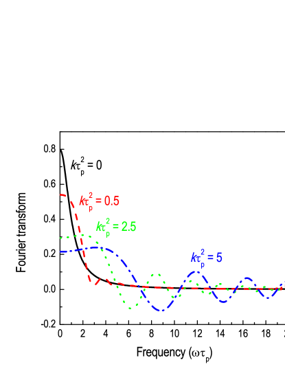
Figure 10: Fourier transform of the pulses given by Eq. (14) for different values of the parameter $k\tau_{\rm p}^{2}=0$ (black/solid), 0.5 (red/dashed), 2.5 (blue/dotted) and 5 (green/dash-dotted) curves, respectively.

Spectral broadening of the pulses results in modifications of the spin coherence initialization and detection. Figure 11 shows the electron spin component after a single pump pulse, $S_{z}^{+}$, as function of magnetic field for different values of the parameter $k$. Spectral broadening of the pulse results in a decrease of the electron spin $z$ component for $\Omega\tau_{\rm pump}=0$ and in a weaker dependence on the magnetic field. As a result, at relatively high magnetic fields the spin coherence generation is more efficient for spectrally wide pulses as compared with Fourier limited pulses because the coherent superposition of the electron spin states is excited more efficiently.

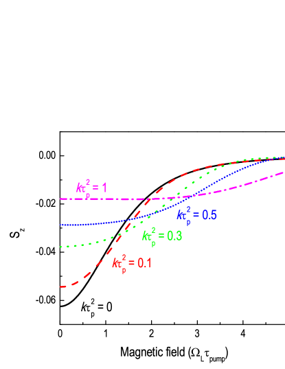
Figure 11: Electron spin $z$ component generated by a single pump pulse as function of magnetic field $\Omega_{\rm L}\tau_{\rm pump}$. Different curves correspond to different spectral widths of the pulse determined by the parameter $k\tau_{\rm pump}^{2}=0$ (black/solid), 0.1 (red/dashed), 0.3 (green/dotted), 0.5 (blue/short dotted), and 1 (magenta/dash dotted).

The spectral dependencies of the ellipticity and Faraday rotation signals are shown in Fig. 12. The red curves correspond to $k\tau_{\rm p}^{2}=0$ and the blue ones to $k\tau_{\rm p}^{2}=1$. For spectrally wide pulse the sensitivities of ellipticity and Faraday rotation do not depend much on the magnetic field, since the solid and dashed curves, corresponding to different values of the field strength, almost coincide. By contrast, the magnetic field effect is strong for spectrally narrow pulses. The appearance of the oscillations in the spectral dependencies for broad pulses are related with the specifics of the pulse Fourier transforms, see oscillations in Fig. 10.

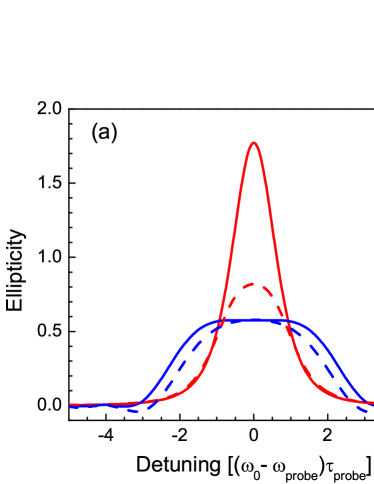
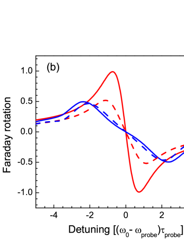
Figure 12: Ellipticity (top) and Faraday rotation (bottom) signals as function of detuning between the QD resonance and the probe optical frequency. The red curves are calculated for $k\tau_{\rm p}^{2}=0$ and the blue ones for $k\tau_{\rm p}^{2}=1$. The solid and dashed sets of curves correspond to two values of magnetic field $\Omega_{\rm L}\tau_{\rm probe}=1.5$ and $0.5$, respectively. The spin $z$ component is the same for all curves. The signals are given in arbitrary units.

Another reason for the spectral broadening of the pump/probe pulses may be related with the jitter of the laser optical frequency. In this case, each pulse generated by the laser is Fourier limited, but its central frequency changes randomly from pulse to pulse. In this case, the theory developed in Sec. IV.1 remains valid, but the results should be averaged over the distribution of the optical frequencies of the laser. Therefore we can safely conclude that the results as derived in the main section will not change for spectrally broadened pulses.

References

- (1) Semiconductor spintronics and quantum computation, edited by D. Awschalom, D. Loss, and N. Samarth (Springer: Berlin, New York, 2002).
- (2) Spin physics in semiconductors, edited by M. Dyakonov (Springer, Berlin, 2008).
- (3) M. V. G. Dutt, J. Cheng, B. Li, X. Xu, X. Li, P. R. Berman, D. G. Steel, A. S. Bracker, D. Gammon, S. E. Economou, R.-B. Liu, and L. J. Sham, Phys. Rev. Lett. 94, 227403 (2005).
- (4) A. Greilich, R. Oulton, E. A. Zhukov, I. A. Yugova, D. R. Yakovlev, M. Bayer, A. Shabaev, A. L. Efros, I. A. Merkulov, V. Stavarache, D. Reuter, and A. Wieck, Phys. Rev. Lett. 96, 227401 (2006).
- (5) A. Greilich, D. R. Yakovlev, A. Shabaev, A. L. Efros, I. A. Yugova, R. Oulton, V. Stavarache, D. Reuter, A. Wieck, and M. Bayer, Science 313, 341 (2006).
- (6) A. Greilich, A. Shabaev, D. R. Yakovlev, A. L. Efros, I. A. Yugova, D. Reuter, A. D. Wieck, and M. Bayer, Science 317, 1896 (2007).
- (7) S. G. Carter, A. Shabaev, S. E. Economou, T. A. Kennedy, A. S. Bracker, and T. L. Reinecke, Phys. Rev. Lett. 102, 167403 (2009).
- (8) T. Auer, R. Oulton, A. Bauschulte, D.R. Yakovlev, M. Bayer, S.Yu. Verbin, R.V. Cherbunin, D. Reuter, and A.D. Wieck, Phys. Rev. B 80, 205303 (2009).
- (9) See, for example, T. Korn, M. Kugler, M. Griesbeck, R. Schulz, A. Wagner, M. Hirmer, C. Gerl, D. Schuh, W. Wegscheider, and C. Schüller, New Journ. Phys. 12, 043003 (2010); D. Brunner, B.D. Gerardot, P.A. Dalgarno, G. Wüst, K. Karrai, N.G. Stoltz, P.M. Petroff, and R.J. Warburton, Science 325 70 (2009).
- (10) X. Marie, T. Amand, P. Le Jeune, M. Paillard, P. Renucci, L. E. Golub, V. D. Dymnikov, and E. L. Ivchenko, Phys. Rev. B 60, 5811 ( 1999).
- (11) I. A. Yugova, M. M. Glazov, E. L. Ivchenko, and A. L. Efros, Phys. Rev. B 80, 104436 (2009).
- (12) M. M. Glazov, I. A. Yugova, S. Spatzek, A. Schwan, S. Varwig, D. R. Yakovlev, D. Reuter, A. D. Wieck, and M. Bayer, Phys. Rev. B 82, 155325 ( 2010).
- (13) A. Shabaev, A. L. Efros, D. Gammon, and I. A. Merkulov, Phys. Rev. B 68, 201305 (2003).
- (14) S. E. Economou, L. J. Sham, Y. Wu, and D. G. Steel, Phys. Rev. B 74, 205415 (2006).
- (15) In the opposite limit the pump and probe pulses can be considered as a constant wave radiation.
- (16) L. Landau and E. Lifshitz, Quantum Mechanics: Non-Relativistic Theory (vol. 3) (Butterworth-Heinemann, Oxford, 1977).
- (17) I. A. Merkulov, A. L. Efros, and M. Rosen, Phys. Rev. B 65, 205309 (2002).
- (18) C. Phelps, T. Sweeney, R. T. Cox, and H. Wang, Phys. Rev. Lett. 102, 237402 (2009).
- (19) E. A. Zhukov, D. R. Yakovlev, M. Bayer, M. M. Glazov, E. L. Ivchenko, G. Karczewski, T. Wojtowicz, and J. Kossut, Phys. Rev. B 76, 205310 (2007).
- (20) N. S. Averkiev and M. M. Glazov, Semiconductors 42, 958 (2008).
- (21) I. A. Yugova, A. A. Sokolova, D. R. Yakovlev, A. Greilich, D. Reuter, A. D. Wieck, and M. Bayer, Phys. Rev. Lett. 102, 167402 (2009).