Thermal noise and dephasing due to electron interactions in non-trivial geometries

Abstract

We study Johnson-Nyquist noise in macroscopically inhomogeneous disordered metals and give a microscopic derivation of the correlation function of the scalar electric potentials in real space. Starting from the interacting Hamiltonian for electrons in a metal and the random phase approximation, we find a relation between the correlation function of the electric potentials and the density fluctuations which is valid for arbitrary geometry and dimensionality. We show that the potential fluctuations are proportional to the solution of the diffusion equation, taken at zero frequency. As an example, we consider networks of quasi-1D disordered wires and give an explicit expression for the correlation function in a ring attached via arms to absorbing leads. We use this result in order to develop a theory of dephasing by electronic noise in multiply-connected systems.

I Introduction

Electronic noise generated by the thermal excitation of charge carriers has been observed and explained by Johnson and Nyquist more than 80 years ago JohnsonNyquist_ThermalAgitation_1928 and discussed in great detail in the literature since then. More recently, it has been found that this so-called Johnson-Nyquist noise is the main source of dephasing in mesoscopic systems at low temperatures of a few Kelvins, where phonons are frozen out. Dephasing puts an IR cut-off for interference phenomena, such as quantum corrections to the classical conductivity.AAK_Localization_1982

The current interest in this topic arises from studies of dephasing in mesoscopic systems which consist of connected quasi-1D disordered wires, Fig. 1, including connected rings and grids. Ferrier_Networks_2004 ; Schopfer_Networks_2007 It has been found (both experimentally Ferrier_Networks_2008 and theoretically Ludwig_Ring_2004 ; Texier_Ring_2004 ; Texier_Multiterminal_2004 ; Treiber_Dephasing_2009 ; Treiber_Book_2010 ) that dephasing depends not only on the dimensionality, but also on the geometry of the system. The noise correlation function is well-understood for macroscopically homogeneous systems such as infinite wires or isolated rings, but has so-far not been studied in multiply-connected networks with leads attached at arbitrary points. The goal of this paper is to give a transparent and systematic description of the thermal noise properties for such systems. In particular, we will derive an expression for the fluctuations of the scalar electric potentials for arbitrary geometries, Eq. (31), and a general expression for the corresponding dephasing rate, Eq. (45). Throughout, we assume that a description of the noise in terms of scalar potentials is sufficient, i.e. we neglect the fluctuations of the transverse component of the electromagnetic field (for a detailed discussion of the latter, see LABEL:AAK_Localization_1982).

Let us start by reviewing simplified arguments to derive the noise correlation function: Johnson and Nyquist concluded that thermal noise in electrical conductors is approximately white, meaning that the power spectral density is nearly constant throughout the whole frequency spectrum. If in addition the fluctuations are uncorrelated for different points in space, a correlation function for the random thermal currents in the classical limit is independent of frequency $\omega$ and momentum ${\bm{q}}$. The power spectrum of the current density reads

$$\langle|{\bm{j}}|^{2}\rangle({\bm{q}},\omega)=2T\sigma_{0}\,.$$ (1)

Here, $\sigma_{0}=e^{2}\nu D$ is the Drude conductivity of the disordered system, $D$ and $\nu$ are the diffusion constant and the density of states, respectively.

Figure 1: A network of wires: We are interested in the noise correlations between arbitrary points ${\bm{x}}$ and ${\bm{y}}$ of multiply-connected networks attached to leads (denoted by the usual ground symbol) at arbitrary points.

Naively applying Ohm’s law, ${\bm{j}}({\bm{q}})=\sigma_{0}{\bm{E}}({\bm{q}})$, to Eq. (1) and using the relation between the electric field and the scalar potential, $e{\bm{E}}({\bm{q}})=-i{\bm{q}}V({\bm{q}})$, we find

$$\langle|V|^{2}\rangle({\bm{q}},\omega)=\frac{2Te^{2}}{\sigma_{0}}\frac{1}{{\bm{q}}^{2}}\,.$$ (2)

The correlation function, Eq. (2), corresponds to the coupling of a given electron to the bath of the surrounding electrons. AAK_Localization_1982 Thus $\langle|V|^{2}\rangle$ describes the process of successive emission and re-absorption of a photon, which is described effectively by the scalar potential $V$. The factor $1/{\bm{q}}^{2}$ coincides with the solution of a diffusion equation in an infinite system, which reflects the fact that the currents, Eq. (1), are uncorrelated in space.

These simple arguments are based on the homogeneity of the system and have assumed a local relation between potential and current, whereas transport properties in disordered metals are substantially non-local. Zyuzin_Fluctuations_1987 ; Kane_Correlations_1988 ; Lerner_CurrentDistribution_1989 ; Texier_Multiterminal_2004 In this paper, we derive an analogy of Eq. (2) for disordered systems with arbitrary geometry and dimensionality; this will in particular apply to networks of disordered wires. A detailed calculation, which takes into account all properties of the mesoscopic samples, has to be done in the real-space representation. Starting points are the usual linear response formalism and the fluctuation-dissipation theorem (FDT). Landau_Book_1980 Although most ingredients of the following discussion will be familiar to experts, we hope that the manner in which they have been assembled here will be found not only to be pedagogically useful, but also helpful for further theoretical studies.

The paper is organized as follows: In Section II, we propose a heuristic description of the potential fluctuations. In Section III, we review a microscopic approach to the noise correlation function, based on a relation of the fluctuations of the scalar potentials to the fluctuations of the density, using the random phase approximation (RPA). In Section IV we evaluate the density response function $\chi$ for disordered systems by using a real-space representation for arbitrary geometries. We apply this result to the noise correlation function in Section V. In Section VI, we show how the noise correlation function can be calculated for networks of disordered wires. Finally, in Section VII we discuss the relation to the fundamental problem of dephasing by electronic interactions.

II Heuristic description of potential fluctuations

A description of fluctuations in metals within the linear response formalism naturally starts with an analysis of the density fluctuations in the model of non-interacting electrons described by the standard free-electron Hamiltonian $\hat{H}^{(0)}$. This system is perturbed by an external scalar potential $V({\bm{x}},t)$ coupled to the density operator $\hat{n}({\bm{x}})$:

$$\hat{H}^{(1)}=\int\!{\rm d}{\bm{x}}\,V({\bm{x}},t)\,\hat{n}({\bm{x}})\,.$$ (3)

The response of the (induced) charge density,

$$n_{\mathrm{ind}}({\bm{x}},\omega) \equiv\int_{-\infty}^{\infty}\!{\rm d}t\,e^{i\omega t}\left[\left\langle\hat{n}({\bm{x}},t)\right\rangle_{\mathrm{pert}}-\left\langle\hat{n}({\bm{x}})\right\rangle\right]$$

$$=-\int\!{\rm d}{\bm{y}}\,\chi({\bm{x}},{\bm{y}},\omega)\,V({\bm{y}},\omega)\,,$$ (4)

is governed by the (retarded) density response function:

$$\chi({\bm{x}},{\bm{y}},\omega) =i\int_{0}^{\infty}\!{\rm d}t\,e^{i(\omega+i0)t}\left\langle[\hat{n}({\bm{x}},t),\hat{n}({\bm{y}},0)]\right\rangle\,.$$ (5)

Here $\left\langle\cdots\right\rangle_{\mathrm{pert}}$ and $\left\langle\cdots\right\rangle$ denote quantum/statistical averaging with respect to the perturbed and unperturbed Hamiltonian, respectively. The FDT relates the equilibrium density fluctuations to the imaginary (dissipative) part of the response function,

$$\langle|n|^{2}\rangle({\bm{x}},{\bm{y}},\omega) \equiv\int_{-\infty}^{\infty}\!{\rm d}t\,e^{i\omega t}\left\langle\hat{n}({\bm{x}},t)\,\hat{n}({\bm{y}},0)\right\rangle$$ (6)

$$=F(\omega)\,{\rm Im}\!\left[\chi({\bm{x}},{\bm{y}},\omega)\right]\,,$$ (7)

where

$$F(\omega)=\frac{2}{1-e^{-\omega/T}}\,.$$ (8)

In writing Eqs. (6)–(8) we have exploited detailed balance and time-reversal symmetry. The latter implies $\chi({\bm{x}},{\bm{y}},\omega)=\chi({\bm{y}},{\bm{x}},\omega)$.Landau_Book_1980

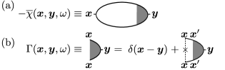
The question which we are going to address in this paper is how to characterize the fluctuations of the electric potential $V$. For this purpose we consider the “dual” case, where some external density $n_{\mathrm{ext}}({\bm{x}},t)$ is the perturbation that couples to the “potential operator” $\hat{V}$:Footnote_VOperator

$$\hat{H}^{(2)}=\int\!{\rm d}{\bm{x}}\,\hat{V}({\bm{x}})\,n_{\mathrm{ext}}({\bm{x}},t)\,.$$ (9)

The linear response of $\hat{V}$ to the perturbation can be written as

$$\langle\hat{V}({\bm{x}},\omega)\rangle_{\mathrm{pert}}=\int\!{\rm d}{\bm{y}}\,\Upsilon({\bm{x}},{\bm{y}},\omega)\,n_{\mathrm{ext}}({\bm{y}},\omega)\,,$$ (10)

defining the response function $\Upsilon$. In analogy to Eq. (7), the response function also characterizes the equilibrium fluctuations of the potential:Footnote_Sign

$$\langle|V|^{2}\rangle({\bm{x}},{\bm{y}},\omega)=F(\omega)\,{\rm Im}\!\left[-\Upsilon({\bm{x}},{\bm{y}},\omega)\right]\,.$$ (11)

Calculating the response function $\Upsilon({\bm{x}},{\bm{y}},\omega)$ is a complicated task because it requires precise knowledge of the potential operator $\hat{V}({\bm{x}})$. Instead, we can identify the potential $V({\bm{x}},\omega)$ in Eq. (4) with the response $\langle\hat{V}({\bm{x}},\omega)\rangle_{\mathrm{pert}}$ in Eq. (10) to relate $\Upsilon$ to $\chi$: In the limit of strong screening in good conductors (called the unitary limit Treiber_Book_2010 ), electroneutrality is satisfied locally. Therefore, the induced charge exactly compensates the external charge: $n_{\mathrm{ind}}({\bm{x}},\omega)=-n_{\mathrm{ext}}({\bm{x}},\omega)$. Now inserting Eq. (4) into Eq. (10) (or vice versa), we obtain

$$\int\!{\rm d}{\bm{x}}^{\prime}\,\Upsilon({\bm{x}},{\bm{x}}^{\prime},\omega)\chi({\bm{x}}^{\prime},{\bm{y}},\omega)=\delta({\bm{x}}-{\bm{y}})\,.$$ (12)

If $\chi$ is known, Eqs. (11) and (12) allow one to calculate the correlation function of the scalar potential.

Let us recall the well-known case of macroscopically homogeneous diffusive systems. The expression for the disordered averaged response function $\overline{\chi}$ readsVollhardt_Localization_1980 ; Akkermans_Book_2007

$$\overline{\chi}({\bm{q}},\omega)=\nu\frac{D{\bm{q}}^{2}}{D{\bm{q}}^{2}-i\omega}=1/\Upsilon({\bm{q}},\omega)\,,$$ (13)

where we used Eq. (12). Inserting Eq. (13) into Eq. (11), we find

$$\langle|V|^{2}\rangle({\bm{q}},\omega)=\frac{1}{\nu}\frac{\omega F(\omega)}{D{\bm{q}}^{2}}\,,$$ (14)

which reduces to Eq. (2) in the limit $\omega\ll T$.

III Noise correlation function for arbitrary geometries: microscopic approach

In Eqs. (3) and (9), we introduced the operators $\hat{n}$ and $\hat{V}$ assuming that either $V({\bm{x}},t)$ or $n_{\mathrm{ext}}({\bm{x}},t)$ are external perturbations. In fact, the fluctuations originate inside of the system and the starting point of a microscopic description is the part of the Hamiltonian, which describes electron interactions,

$$\hat{H}_{\rm int}=\int\!{\rm d}{\bm{x}}\,\!{\rm d}{\bm{y}}\,U_{0}({\bm{x}},{\bm{y}})\hat{\psi}^{\dagger}({\bm{x}})\hat{\psi}^{\dagger}({\bm{y}})\hat{\psi}({\bm{y}})\hat{\psi}({\bm{x}})\,,$$ (15)

where $U_{0}({\bm{x}},{\bm{y}})$ is the bare Coulomb interaction. In the mean-field approximation, Eq. (15) gives rise to a correction, called Hartree contribution, to the electron energy:

$$\Delta E^{(\mathrm{Hartree})}\approx\int\!{\rm d}{\bm{x}}\,\!{\rm d}{\bm{y}}\,U_{0}({\bm{x}},{\bm{y}})\langle\hat{n}({\bm{x}})\rangle\langle\hat{n}({\bm{y}})\rangle\,,$$ (16)

where $\hat{n}({\bm{x}})=\hat{\psi}^{\dagger}({\bm{x}})\hat{\psi}({\bm{x}})$.

Figure 2: The Coulomb interaction in the RPA according to Eq. (17).

The Coulomb interactions are dynamically screened, which can be accounted for in the framework of the RPA, provided that the electron density is high,

$$U_{{\rm RPA}}({\bm{x}},{\bm{y}},\omega)=U_{0}({\bm{x}},{\bm{y}})-\int\!{\rm d}{\bm{x}}^{\prime}\,\!{\rm d}{\bm{y}}^{\prime}\,U_{0}({\bm{x}},{\bm{x}}^{\prime})\chi({\bm{x}}^{\prime},{\bm{y}}^{\prime},\omega)$$

$$\qquad\qquad\qquad\qquad\times U_{{\rm RPA}}({\bm{y}}^{\prime},{\bm{y}},\omega)\,,$$ (17)

see Fig. 2. Note that $-\chi$ [see the definition in Eq. (5)] is equal to the bubble diagrams of Fig. 2, see e.g. LABEL:Akkermans_Book_2007. In Appendix A, we recall how to obtain Eq. (17) within a self consistent treatment of the screening problem.

Using the RPA in Eq. (16) and comparing the result with equation Eq. (9), we observe that the potential fluctuations are due to electronic interactions and that the operator of the scalar potential is given by

$$\hat{V}({\bm{x}},\omega)=\int\!{\rm d}{\bm{y}}\,U_{{\rm RPA}}({\bm{x}},{\bm{y}},\omega)\,\hat{n}({\bm{y}})\,.$$ (18)

Eq. (18) allows us to relate the correlation function of the potentials to the correlation function of the density fluctuations:

$$\langle|V|^{2}\rangle({\bm{x}},{\bm{y}},\omega)=\int\!{\rm d}{\bm{x}}^{\prime}\,\!{\rm d}{\bm{y}}^{\prime}\,U_{{\rm RPA}}({\bm{x}},{\bm{x}}^{\prime},\omega)$$

$$\qquad\qquad\qquad\quad\ \times\langle|n|^{2}\rangle({\bm{x}}^{\prime},{\bm{y}}^{\prime},\omega)U_{{\rm RPA}}^{*}({\bm{y}}^{\prime},{\bm{y}},\omega)\,.$$ (19)

By inserting Eqs. (17) and (7) into Eq. (19), re-ordering the terms in the RPA series and using the fact that $U_{0}$ is real, we find (see Fig. 3)

$$\langle|V|^{2}\rangle({\bm{x}},{\bm{y}},\omega)=F(\omega)\,{\rm Im}\!\left[-U_{{\rm RPA}}({\bm{x}},{\bm{y}},\omega)\right]\,.$$ (20)

We emphasize that the derivation of Eq. (20) has not used any other assumption than the RPA. Thus, Eqs. (17) and (20) are a microscopic (and more rigorous) counterpart of the phenomenological Eqs. (11) and (12).

Figure 3: Diagrammatic proof of Eq. (20) by using Eq. (19) and Eq. (17) (i.e. Fig. 2).

IV Density response in disordered systems: calculations in coordinate representation

In disordered metals the motion of the electrons is diffusive, provided that $k_{F}^{-1}\ll\ell\ll L$ where $k_{F}$ is the Fermi wave-vector, $\ell$ the mean free path and $L$ the system size. It can be accounted for by substituting the disorder-averaged density response function, $\overline{\chi}$, into the phenomenological Eqs. (11) and (12) or the microscopic Eqs. (17) and (20). The function $\overline{\chi}$ has been calculated for macroscopically homogeneous systems by Vollhardt and Wölfle. Vollhardt_Localization_1980 In the following, we will show how to generalize their calculation to inhomogeneous systems. A useful starting point is a coordinate representation of the density response function, Eq. (5), in terms of the advanced and retarded Green’s functions, $G^{R/A}({\bm{x}},{\bm{y}},\omega)$,

$$\overline{\chi}({\bm{x}},{\bm{y}},\omega)= \frac{1}{2\pi i}\int\!{\rm d}\epsilon\,\Big{(}\left[f(\epsilon+\omega)-f(\epsilon)\right]$$ (21)

$$\times\overline{G^{R}({\bm{x}},{\bm{y}},\epsilon+\omega)G^{A}({\bm{y}},{\bm{x}},\epsilon)}$$

$$+f(\epsilon)\overline{G^{R}({\bm{x}},{\bm{y}},\epsilon+\omega)G^{R}({\bm{y}},{\bm{x}},\epsilon)}$$

$$-f(\epsilon+\omega)\overline{G^{A}({\bm{x}},{\bm{y}},\epsilon+\omega)G^{A}({\bm{y}},{\bm{x}},\epsilon)}\Big{)}\,,$$

see Fig. 4(a). Here, $f(\omega)$ is the Fermi distribution function, and $\overline{\cdots}$ denotes disorder averaging. The combinations $\overline{G^{R}G^{R}}$ and $\overline{G^{A}G^{A}}$ give short-range contributions, since the average of the products decouple, e.g. $\overline{G^{R}G^{R}}\simeq\overline{G^{R}}\cdot\overline{G^{R}}+{\cal O}(1/k_{F}\ell)$, and the disorder averaged Green’s functions $\overline{G^{R}}$ and $\overline{G^{A}}$ decay on the scale $\ell\ll L$. We will consider contributions to the thermal noise which are governed by distances larger than $\ell$, cf. LABEL:AAK_Localization_1982. Therefore, details of the behavior on short scales are not important for our purposes and we replace the short-range contributions, $\overline{G^{R}G^{R}}$ and $\overline{G^{A}G^{A}}$, by a delta function.

Figure 4: (a) Equation for the disorder averaged density response function; solid lines denote the disorder averaged retarded and/or advanced Green functions, cf. Eq. (21). (b) Equation for the impurity vertex; the dashed line represents impurity scattering, cf. Eq. (23).

The long range contributions $\overline{G^{R}G^{A}}$ can be calculated by standard methods,Akkermans_Book_2007

$$\overline{G^{R}({\bm{x}},{\bm{y}},\epsilon+\omega)G^{A}({\bm{y}},{\bm{x}},\epsilon)}=\int\!{\rm d}{\bm{x}}^{\prime}\,\overline{G^{R}}({\bm{x}},{\bm{x}}^{\prime},\epsilon+\omega)$$

$$\qquad\qquad\qquad\qquad\qquad\times\overline{G^{A}}({\bm{x}}^{\prime},{\bm{x}},\epsilon)\Gamma({\bm{x}}^{\prime},{\bm{y}},\omega)\,,$$ (22)

where $\Gamma({\bm{x}},{\bm{y}},\omega)$ is the impurity vertex function,

$$\Gamma({\bm{x}},{\bm{y}},\omega) =\delta({\bm{x}}-{\bm{y}})+\frac{1}{2\pi\nu\tau}\!\!\int\!{\rm d}{\bm{x}}^{\prime}\,\overline{G^{R}}({\bm{x}},{\bm{x}}^{\prime},\epsilon+\omega)$$

$$\qquad\times\overline{G^{A}}({\bm{x}}^{\prime},{\bm{x}},\epsilon)\Gamma({\bm{x}}^{\prime},{\bm{y}},\omega)$$ (23)

(the factor $1/2\pi\nu\tau$, where $\tau=\ell/v_{F}$ is the transport time, originates from the impurity line), see Fig. 4(b). The short-ranged product, $\overline{G^{R}}\cdot\overline{G^{A}}$, can be expanded as $\overline{G^{R}}\cdot\overline{G^{A}}\simeq 2\pi\nu\tau\,\delta({\bm{x}}-{\bm{x}}^{\prime})\big{[}1+i\omega\tau+\tau D\Delta_{{\bm{x}}}\big{]}$, which is obtained by transforming the product to momentum space and expanding in the transferred momentum ${\bm{q}}$ and frequency $\omega$, realizing that terms of order ${\bm{q}}$ vanish due to symmetry. As a result, Eq. (23) reduces to a diffusion equation:

$$\left(-i\omega-D\Delta_{{\bm{x}}}\right)\Gamma({\bm{x}},{\bm{y}},\omega)=\frac{1}{\tau}\delta({\bm{x}}-{\bm{y}})\,,$$ (24)

where $D=v_{F}\ell/d$ is the diffusion constant for a $d$ dimensional system. Thus, the vertex function is proportional to the diffusion propagator, $\Gamma({\bm{x}},{\bm{y}},\omega)=P({\bm{x}},{\bm{y}},\omega)/\tau$.

Collecting the short- and long-range contributions and taking the limit $T\ll\epsilon_{F}$, we obtain from Eq. (21)

$$\overline{\chi}({\bm{x}},{\bm{y}},\omega)=\nu\left(\delta({\bm{x}}-{\bm{y}})+i\omega P({\bm{x}},{\bm{y}},\omega)\right)\,.$$ (25)

Eq. (25) is valid for arbitrary geometries since it is based only on the diffusive approximation and does not require macroscopic homogeneity.

V Noise correlation function in disordered systems

Let us simplify Eq. (17) for a disordered conductor. Using Eq. (25) and

$$-\frac{1}{4\pi e^{2}}\Delta_{\bm{x}}U_{0}({\bm{x}},{\bm{x}}^{\prime})=\delta({\bm{x}}-{\bm{x}}^{\prime})\,,$$ (26)

Eq. (17) can be written as

$$\left(1-\frac{\Delta_{\bm{x}}}{\kappa^{2}}\right)U_{{\rm RPA}}({\bm{x}},{\bm{y}},\omega)+i\omega\int\!{\rm d}{\bm{x}}^{\prime}\,P({\bm{x}},{\bm{x}}^{\prime},\omega)$$

$$\quad\times U_{{\rm RPA}}({\bm{x}}^{\prime},{\bm{y}},\omega)=\frac{1}{\nu}\delta({\bm{x}}-{\bm{y}})\,,$$ (27)

where we introduced the Thomas-Fermi screening wave-vector $\kappa=\sqrt{4\pi e^{2}\nu}$, which corresponds to the inverse screening length in three dimensional (3D) bulk systems. The kernel of Eq. (27) is a solution to the diffusion equation (24) which can be expanded in terms of eigenfunctions of the Laplace operator. Consequently, the kernel is always separable and Eq. (27) has a unique solution (see e.g. LABEL:Kanwal_IntegralEquations_1997 for details on how the solution can be found). Using the semi-group property of the diffusion propagators,

$$\int\!{\rm d}{\bm{x}}^{\prime}\,P({\bm{x}},{\bm{x}}^{\prime},\omega)P({\bm{x}}^{\prime},{\bm{y}},0)=\frac{i}{\omega}\left[P({\bm{x}},{\bm{y}},0)-P({\bm{x}},{\bm{y}},\omega)\right]\,,$$

one can check that

$$U_{{\rm RPA}}\!({\bm{x}},{\bm{y}},\omega)\!=\!\frac{1}{\nu}\!\left(\!\frac{1}{-D\Delta_{\bm{x}}-i\omega}\!+\!\frac{1}{D\kappa^{2}}\!\right)^{\!\!\!-1}\!\!\!P({\bm{x}},{\bm{y}},0)$$ (28)

satisfies Eq. (27). In practice, the 3D Thomas-Fermi screening length $\kappa^{-1}$ is a microscopic scale, thus the typical value of the first term of the rhs. of Eq. (28), $(D{\bm{q}}^{2}_{{\rm typ}}-i\omega_{{\rm typ}})^{-1}$, is larger than $1/D\kappa^{2}=1/4\pi\sigma_{0}$ for good conductors (this is the so-called unitary limit, for details see LABEL:Treiber_Book_2010):

$$\frac{1}{|D{\bm{q}}^{2}_{{\rm typ}}-i\omega_{{\rm typ}}|}\gg\frac{1}{D\kappa^{2}}\,.$$ (29)

In this limit, using the diffusion Eq. (24), we obtain from Eq. (28):

$$U_{{\rm RPA}}({\bm{x}},{\bm{y}},\omega)=\frac{1}{\nu}\left[\delta({\bm{x}}-{\bm{y}})-i\omega P({\bm{x}},{\bm{y}},0)\right]\,.$$ (30)

We remind that $P({\bm{x}},{\bm{y}},0)$ is always real. As a result, Eqs. (20) and (30) yield

$$\langle|V|^{2}\rangle({\bm{x}},{\bm{y}},\omega)=\frac{1}{\nu}\,\omega F(\omega)P({\bm{x}},{\bm{y}},0)\,,$$ (31)

where $F(\omega)$ is given by Eq. (8). The real-space demonstration of Eqs. (30) and (31) for macroscopically inhomogeneous systems, are among the main results of the paper. It is worth emphasizing the frequency-space factorization of the correlator, which plays an important role in the theory of dephasing, cf. Section VII. The relation of Eq. (31) to the correlation function of the currents, Eq. (1), is discussed in Appendix B, and allows to put the presentation of the introduction on firm ground.

Note that Eq. (29) allows one to neglect the term $\Delta_{\bm{x}}/\kappa^{2}$ in Eq. (27) and, thus, to reduce Eq. (27) to the form of the phenomenological integral equation (12), with $U_{{\rm RPA}}$ taking the place of $\Upsilon$. [The same replacement leads from Eq. (11) to Eq. (20).] In other words, the electric potential of the fluctuating charge densities itself is negligible when screening is strong enough (i.e. good conductors in the unitary limit), justifying a posteriori our assumptions in the phenomenological Section II.

The fact that the correlation function of the potential is proportional to the solution of the diffusion equation at zero frequency, cf. Eq. (31), may be understood as a non-local version of the Johnson-Nyquist theorem, since $P({\bm{x}},{\bm{y}},0)$ can be related to the classical dc-resistance $\mathcal{R}({\bm{x}},{\bm{y}})$ between the points ${\bm{x}}$ and ${\bm{y}}$ (see LABEL:Texier_NetworksCylinders_2009):

$$\mathcal{R}({\bm{x}},{\bm{y}})=\frac{2D}{\sigma_{0}}\left\{\frac{1}{2}\big{[}P({\bm{x}},{\bm{x}},0)+P({\bm{y}},{\bm{y}},0)\big{]}-P({\bm{x}},{\bm{y}},0)\right\}\,.$$ (32)

For example, in an infinitely long quasi-1D wire of cross-section $s$, the solution of the diffusion equation is $P({\bm{x}},{\bm{y}},0)=-|x-y|/(Ds)$ where $x$ is the component of ${\bm{x}}$ along the wire. Hence we recover a resistance proportional to the distance between the points, $\mathcal{R}({\bm{x}},{\bm{y}})=|x-y|/(s\sigma_{0})$.

VI Noise correlation function in networks of disordered wires

Let us now illustrate the calculation of the noise correlation function, Eq. (31), for a network of disordered wires. The main ingredient to Eq. (31) is the solution of the diffusion equation (24) at zero frequency. Wires allow a quasi-1D description of diffusion, where transverse directions can be integrated out since $P({\bm{x}},{\bm{y}},\omega)$ is assumed to be constant on the scale of the width of the wire. As a result, we replace $P({\bm{x}},{\bm{y}},\omega)\to P(x,y,\omega)/s$, where $s$ is the cross-section of the wires and $P(x,y,\omega)$ solves the 1D diffusion equation in the network, $x$ and $y$ being coordinates along the wires. Recently, effective methods have been developed to solve the resulting diffusion equation for arbitrary networks.Texier_Multiterminal_2004 ; Pascaud_PersistentCurrents_1999 ; Akkermans_SpectralDeterminant_2000 ; Texier_NetworksCylinders_2009 We will review these methods in this Section and evaluate the noise correlation function for a simple example.

We start by introducing some basic notations: A network is a set of vertices, labeled by an index $\alpha$, connected via wires of arbitrary length, say $l_{\alpha\beta}$ for the wire connecting vertices $\alpha$ and $\beta$. Let us define a vertex matrix $\mathcal{M}$ as

$$\mathcal{M}_{\alpha\beta}=\delta_{\alpha\beta}\sum_{\gamma}\frac{a_{\alpha\gamma}}{l_{\alpha\gamma}}-\frac{a_{\alpha\beta}}{l_{\alpha\beta}}\,,$$ (33)

where $a_{\alpha\beta}=1$ if the vertices $\alpha$ and $\beta$ are connected and $a_{\alpha\beta}=0$ otherwise. The solution of the diffusion equation at zero frequency between arbitrary vertices $\alpha,\beta$ of the network is given by the entries of the inverse matrix ${\cal M}$ divided by the diffusion constant:

$$P(\alpha,\beta,0)=({\cal M}^{-1})_{\alpha\beta}/D\,.$$ (34)

This allows us to calculate the noise correlation function between arbitrary points of a network by inserting vertices and inverting ${\cal M}$. As an aside, note that arbitrary boundary conditions can be included in this scheme easily (see Refs. [Akkermans_SpectralDeterminant_2000, ; Texier_NetworksCylinders_2009, ] for details).

Let us consider the network shown in Fig. 5, representing a ring connected to absorbing leads.

Figure 5: The network corresponding to a symmetric ring made of four wires connected to two absorbing leads. The length of the arcs is $l$ and the length of the connecting arms is $b$. Vertices are labeled by numbers $\alpha=1,2,3,4$. Vertices “$1$” and “$4$” denote the points where the ring is connected to the arms. Vertex “$2$” is always placed in the upper arc, defining the running coordinate $x$. Vertex “$3$” determines the $y$-coordinate and is placed either in the adjacent arc (panel a) or in the left arc (panel b) or in the same arc (panel c).

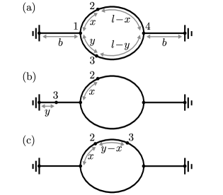
For simplicity, we assumed that the ring is symmetric: the two arcs are of the same length $l$ and the connecting arms of length $b$. We evaluate the noise correlation function for two points in this network by inserting two vertices, called “$2$” and “$3$”. Vertex “$2$” is always placed in the upper arc, encoding the running coordinate $x$ in the length of the connected wires. Vertex “$3$” determines the $y$-coordinate and is placed either in the lower arc or in the left connecting arm or in the upper arc. In the first case, Fig. 5(a), the vertex matrix, Eq. (33), is given by

$${\mathcal{M}}\!=\!\begin{pmatrix}\frac{1}{b}\!+\!\frac{1}{x}\!+\!\frac{1}{y}&-\frac{1}{x}&-\frac{1}{y}&0\\ -\frac{1}{x}&\frac{1}{x}\!+\!\frac{1}{l-x}&0&-\frac{1}{l-x}\\ -\frac{1}{y}&0&\frac{1}{y}\!+\!\frac{1}{l-y}&-\frac{1}{l-y}\\ 0&-\frac{1}{l-x}&-\frac{1}{l-y}&\frac{1}{b}\!+\!\frac{1}{l-x}\!+\!\frac{1}{l-y}\end{pmatrix}.$$ (35)

The diffusion propagator is then given by $P(x,y,0)=(\mathcal{M}^{-1})_{23}/D$, and we obtain from Eq. (31) the correlation function as a function of the running coordinates $x$, $y$ $\in[0,l]$:

$$\langle|V|^{2}\rangle(x,y,\omega)= \frac{\omega F(\omega)}{D\nu s}\frac{b(l(2b+l)-(x+y)l+2xy)}{l(4b+l)}\,.$$ (36)

When vertex “$3$” is placed in the connecting arm, $x\in[0,l]$ and $y\in[0,b]$ [Fig. 5(b)], we get

$$\langle|V|^{2}\rangle(x,y,\omega)=\frac{\omega F(\omega)}{D\nu s}\frac{y(2b+l-x)}{4b+l}\,.$$ (37)

Finally, when vertex “$3$” is placed in the same arc of the ring as vertex “$2$” [see Fig. 5(c)], following the same logic we obtain, with $0<x<y<l$,

$$\langle|V|^{2}\rangle(x,y,\omega)$$

$$=\frac{\omega F(\omega)}{D\nu s}\frac{bl(2b+l)+xl(3b+l)-ybl-xy(2b+l)}{l(4b+l)}\,.$$ (38)

All other configurations can be found by symmetry arguments.

Figure 6: (color online) The solution to the diffusion equation at zero frequency, $P(x,y,0)\propto\langle|V|^{2}\rangle(x,y,\omega)$, where $\langle|V|^{2}\rangle$ is given by Eqs. (36)–(38), for a fixed coordinate $x$ in the upper arm of the ring (indicated by the dot), as a function of $y$ traversing the network. $\langle|V|^{2}\rangle(x,y,\omega)$ is linear in $y$ and its derivative has a discontinuity at $y=x$.

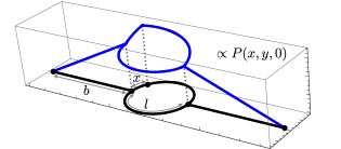
We plot $P(x,y,0)$ for $y$ traversing the whole network in Fig. 6. Note that the resulting function is linear in $y$ and its derivative has a discontinuity at $y=x$ (cf. LABEL:Texier_Ring_2004).

VII Application to dephasing

The precise characterization of potential fluctuations is very important in studying phase coherent properties of disordered metals at low temperatures. To be specific, let us discuss a particular coherent property: the weak localization correction to the conductivity. Let us recall that the weak localization (WL) correction $\Delta\sigma\equiv\overline{\sigma}-\sigma_{0}$ is a small contribution to the averaged conductivity arising from quantum interference of reversed diffusive electronic trajectories.Khmelnitskii_1984

At low temperatures, dephasing is dominated by electron interactions, that can be accounted for through a contribution to the phase accumulated by two time-reversed interfering trajectories in a fluctuating electric field AAK_Localization_1982 :

$$\Phi[{\bm{x}}(\tau)]=\int_{0}^{t}\!{\rm d}\tau\,\,\big{[}V({\bm{x}}(\tau),\tau)-V({\bm{x}}(\tau),t-\tau)\big{]}\,.$$ (39)

When averaged over the Gaussian fluctuations of the electric field, $\langle e^{i\Phi}\rangle_{V}=e^{-\frac{1}{2}\langle{\Phi^{2}}\rangle_{V}}$ yields a phase difference which cuts off the contributions of long electronic trajectories. Introducing the trajectory-dependent dephasing rate $\Gamma[{\bm{x}}(\tau)]=\frac{1}{2t}\langle\Phi[{\bm{x}}(\tau)]^{2}\rangle_{V}$, the weak localization correction takes the form:Texier_Ring_2004 ; Montambaux_QuasiparticleDecay_2005 ; Marquardt_Decoherence_2007 ; Texier_NetworksCylinders_2009

$$\Delta\sigma({\bm{x}})=-\frac{2e^{2}D}{\pi}\int_{0}^{\infty}\!{\rm d}t\,\,P({\bm{x}},{\bm{x}},t)\,\langle e^{-t\Gamma[{\bm{x}}(\tau)]}\rangle_{\{{\bm{x}}(\tau)\}}\,,$$ (40)

where $\langle\cdots\rangle_{\{{\bm{x}}(\tau)\}}$ is the average with respect to closed diffusive trajectories of duration $t$ starting from ${\bm{x}}$ (not to be confused with the thermal average $\left\langle\cdots\right\rangle_{V}$ over the electric potential $V$). The phase fluctuations can then be related to the potential fluctuations:

$$\frac{1}{2}\langle\Phi[{\bm{x}}]^{2}\rangle=\int_{0}^{t}\!{\rm d}\tau\,\!{\rm d}\tau\,^{\prime}\int_{-\infty}^{\infty}\frac{\!{\rm d}\omega\,}{2\pi}\left[e^{-i\omega(\tau-\tau^{\prime})}-e^{-i\omega(\tau+\tau^{\prime}-t)}\right]$$

$$\qquad\qquad\qquad\times\langle|V|^{2}\rangle_{\varphi}({\bm{x}}(\tau),{\bm{x}}(\tau^{\prime}),\omega)\,.$$ (41)

Here we have introduced a new noise correlator,

$$\langle|V|^{2}\rangle_{\varphi}({\bm{x}},{\bm{y}},\omega)=\frac{1}{\nu}\,\omega F_{\varphi}(\omega)P({\bm{x}},{\bm{y}},0)\,,$$ (42)

obtained from Eq. (31) by replacing $F(\omega)$ with a modified function $F_{\varphi}(\omega)$ (given below), on the origin of which we now comment. Equation (20) is well-known in the theory of dephasing: its version symmetrized with respect to frequency arises naturally when comparing the diagrammatic calculation of the dephasing time Aleiner_DisorderedSystems_1986 ; vonDelft_Decoherence_2007 with the influence functional approach describing electrons moving in a random Gaussian field $V$. Chakravarty_WeakLocalization_1986 ; Marquardt_Decoherence_2007 ; vonDelft_InfluenceFunctional_2008 Diagrammatically, the symmetrized Eq. (20) represents the Keldysh component of the screened electron interaction propagator, the only substantial difference being that the diagrammatically calculated correlation function involved in the dephasing process acquires so-called “Pauli-factors” that account for the fact that the Fermi sea limits the phase space available for inelastic transitions. vonDelft_InfluenceFunctional_2008 These factors lead to the following replacement of the function $F(\omega)$ in Eq. (20) and here also in Eq. (31):

$$F(\omega)\overset{\mathrm{sym}}{\longrightarrow}\coth(\omega/2T)\overset{\mathrm{Pauli}}{\longrightarrow}\frac{\omega/2T}{\sinh^{2}(\omega/2T)}\equiv F_{\varphi}(\omega)\,.$$ (43)

This restricts the energy transfer to $|\omega|<T$, Marquardt_Decoherence_2007 ; vonDelft_Decoherence_2007 but does not affect the factorization of the correlator. Inserting Eq. (42) into Eq. (41) leads to

$$\frac{1}{2}\langle\Phi[{\bm{x}}]^{2}\rangle=\frac{2T}{\nu}\int_{0}^{t}\!{\rm d}\tau\,\!{\rm d}\tau\,^{\prime}\,P({\bm{x}}(\tau),{\bm{x}}(\tau^{\prime}),0)\int_{-\infty}^{\infty}\frac{\!{\rm d}\omega\,}{2\pi}$$

$$\qquad\qquad\times\left[e^{-i\omega(\tau-\tau^{\prime})}-e^{-i\omega(\tau+\tau^{\prime}-t)}\right]\frac{\omega}{2T}F_{\varphi}(\omega)\,.$$ (44)

The fact that the frequency dependent function $\frac{\omega}{2T}F_{\varphi}(\omega)$ is symmetric allows us to add to $P({\bm{x}}(\tau),{\bm{x}}(\tau^{\prime}),0)$ the term $-\frac{1}{2}\big{[}P({\bm{x}}(\tau),{\bm{x}}(\tau),0)+P({\bm{x}}(\tau^{\prime}),{\bm{x}}(\tau^{\prime}),0)\big{]}$, which does not contribute to the integral (44). Therefore we finally end up with the following expression for the dephasing rate,

$$\Gamma[{\bm{x}}(\tau)] =e^{2}T\int_{0}^{t}\frac{\!{\rm d}\tau\,}{t}\int_{0}^{t}\!{\rm d}\tau\,^{\prime}\,\left[\delta_{T}(\tau+\tau^{\prime}-t)-\delta_{T}(\tau-\tau^{\prime})\right]$$

$$\qquad\times\mathcal{R}\left({\bm{x}}(\tau),{\bm{x}}(\tau^{\prime})\right)\,,$$ (45)

written in terms of the resistance $\mathcal{R}$, defined in Eq. (32). The function $\delta_{T}(t)$, a broadened delta function of width $1/T$ and height $T$, is the Fourier transform of $\frac{\omega}{2T}F_{\varphi}(\omega)$, which is given by

$$\delta_{T}(\tau)=\pi T\,w(\pi T\tau)\,,\quad w(y)=\frac{y\coth y-1}{\sinh^{2}y}\,.$$ (46)

Eq. (45), which is one of the main results of our paper, generalizes the results obtained in Refs. [Marquardt_Decoherence_2007, ; Treiber_Book_2010, ; Treiber_Dephasing_2009, ; vonDelft_InfluenceFunctional_2008, ] for an infinite wire and an isolated ring to arbitrary geometry. In the classical noise limit, $T\to\infty$, $\delta_{T}(\tau)$ may be replaced by a $\delta(\tau)$ function: The second term of Eq. (45) vanishes and we recover the results of Refs. [Texier_Ring_2004, ; Texier_NetworksCylinders_2009, ].

Let us now illustrate Eq. (45) by calculating the dephasing time for the well-understood case of one and two-dimensional isolated simply-connected samples. The dephasing time can be extracted from the condition

$$1\equiv\Gamma(\tau_{\varphi})\tau_{\varphi}\,,$$ (47)

where $\Gamma(t)$ is given by the functional Eq. (45), averaged over the typical closed random walks ${\bm{x}}(\tau)$ of duration $t$ in the system. The problem is governed by the interplay of three time-scales: The Thouless time $\tau_{\rm Th}=L^{2}/D$, depending on the system size $L$, the thermal time $\tau_{T}=1/T$ (related to the thermal length $L_{T}=\sqrt{D/T}$), and the dephasing time $\tau_{\varphi}$.

(i) Diffusive regime, $\tau_{T}\ll\tau_{\varphi}\ll\tau_{\rm Th}$ ($L_{T}\ll L_{\varphi}\ll L$): this is the regime considered in Refs. [AAK_Localization_1982, ; Montambaux_QuasiparticleDecay_2005, ], where the width of the broadened delta functions in Eq. (45), $\tau_{T}$, is the shortest time-scale. Thus, when averaging over paths ${\bm{x}}(\tau)$, the characteristic length-scale $|x-y|$ entering the resistance $\mathcal{R}(x,y)$ can be determined as follows: For the first $\delta_{T}$ term this length is governed by free diffusion, since $|{\bm{x}}(\tau)-{\bm{x}}(t-\tau)|\sim\sqrt{D\tau}$, hence $|x-y|\sim\sqrt{D\tau}$. For the second term the characteristic length is set by the width of the delta function, $|x-y|\sim\sqrt{D\tau_{T}}$. In 1D, where $\mathcal{R}(x,y)\sim|x-y|/\sigma_{0}s$, the first term dominates and we immediately obtain from Eq. (47) $1/\tau_{\varphi}\sim(e^{2}\sqrt{D}T/\sigma_{0}s)^{2/3}$. In 2D, the diffuson at zero frequency is logarithmic as well as the resistance (32), $\mathcal{R}(x,y)\sim\ln(|x-y|)/\sigma_{0}d$, where $d$ is the width of the sample, which can be understood from the fact that the resistance of a plane connected at two corners scales logarithmically with the system size. Eq. (47) gives $1\sim e^{2}T\tau_{\varphi}\ln(T\tau_{\varphi})/\sigma_{0}d$, and for the dephasing time: $1/\tau_{\varphi}\sim e^{2}T\ln(e^{2}/\sigma_{0}d)/\sigma_{0}d$.

(ii) Ergodic regime, $\tau_{T}\ll\tau_{\rm Th}\ll\tau_{\varphi}$ ($L_{T}\ll L\ll L_{\varphi}$): the width of $\delta_{T}(\tau)$ in Eq. (45) is still the shortest time-scale but, in contrast to (i), the typical trajectories ${\bm{x}}(\tau)$ explore the whole system, setting the length-scale of diffusion to the system size $L$, cf. Refs. [Ludwig_Ring_2004, ; Texier_Ring_2004, ]. In full analogy to the diffusive regime, but replacing $\sqrt{D\tau}$ by $L$, we find for 1D, $1/\tau_{\varphi}\sim e^{2}LT/\sigma_{0}s$, and for 2D, $1/\tau_{\varphi}\sim e^{2}T\ln(\tau_{\rm Th}/\tau_{T})/\sigma_{0}d$.Takane These examples show that for non-trivial geometries dephasing due to electron interactions cannot be accounted for through a unique dephasing rate depending only on dimensionality, but must be described by a functional of the trajectories ${\bm{x}}(\tau)$ since the qualitative behavior of $\tau_{\varphi}$ follows from the geometry dependent typical distance $|{\bm{x}}(\tau)-{\bm{x}}(\tau^{\prime})|$.

For sufficiently low temperatures, on the other hand, Eq. (45) is capable to describe the crossover to a 0D regime, where, apart from a dependence on the total system size, geometry becomes unimportant:

(iii) 0D regime, $\tau_{\rm Th}\ll\tau_{T}\ll\tau_{\varphi}$ ($L\ll L_{T}\ll L_{\varphi}$): here, the width of the delta functions in Eq. (45), $\tau_{T}$, is larger than $\tau_{\rm Th}$. Hence, the trajectories reach the ergodic limit ${\bm{x}}(\tau\geq\tau_{\rm Th})\sim L$ before the electric potential has significantly changed: Dephasing is strongly reduced. Let us denote the maximal resistance reached at the ergodic limit as $\mathcal{R}_{\rm erg}$ and replace the resistance in Eq. (45) by $\mathcal{R}\to\mathcal{R}-\mathcal{R}_{\rm erg}$, without changing the result, since $\mathcal{R}_{\rm erg}$ is constant and its contribution vanishes after integrating over $\tau$ and $\tau^{\prime}$. The difference $\mathcal{R}-\mathcal{R}_{\rm erg}$ is nonzero only during time differences $\tau-\tau^{\prime}\lesssim\tau_{\rm Th}$, before reaching ergodicity. Thus, the leading contribution comes from the second $\delta_{T}$ term in Eq. (45), which is constant at its maximum $T$ during such short time-scales. We find $1\sim-e^{2}T^{2}\tau_{\varphi}\int_{0}^{\tau_{\rm Th}}\!{\rm d}\tau\,[\mathcal{R}({\bm{x}}(\tau),0)-\mathcal{R}_{\rm erg}]$ and since the $\mathcal{R}_{\rm erg}$ term dominates, we obtain a dephasing time $1/\tau_{\varphi}\sim e^{2}T^{2}\tau_{\rm Th}\mathcal{R}_{\rm erg}$, independent of geometry and with the characteristic $\sim T^{2}$ behavior. Sivan_QuasiParticleLifetime_1994

VIII Conclusions

In this paper we have considered fluctuations of the scalar electric potentials in macroscopically inhomogeneous metals. We have shown how to relate the density fluctuations to the potential fluctuations, emphasizing the role of electronic interactions, provided a real space derivation of the density response function and illustrated these general ideas for the case of networks of metallic wires. Finally we have obtained a trajectory-dependent functional, Eq. (45), which describes dephasing by electron interactions for arbitrary geometries and accounts for the quantum noise contribution. When applied to networks, Eq. (45) can describe the full crossover from the 0D to the 1D and the 2D regime.

Appendix A Self consistent analysis of screening

We recall here how to obtain Eq. (17) using a self-consistent treatment of screening in real space.Christen_Buttiker_1996 Starting points are the following three equations: (i) the excess charge density is decomposed into external and induced contributions

$$\delta n({\bm{x}},\omega)=n_{\mathrm{ext}}({\bm{x}},\omega)+n_{\mathrm{ind}}({\bm{x}},\omega)\,.$$ (48)

(ii) The induced charge is related to the potential $V({\bm{x}},\omega)$ by the density response function, cf. Eq. (4):

$$n_{\mathrm{ind}}({\bm{x}},\omega)=-\int\!{\rm d}{\bm{y}}\,\,\chi({\bm{x}},{\bm{y}},\omega)\,V({\bm{y}},\omega)\,.$$ (49)

(iii) The Poisson equation

$$\Delta\,V({\bm{x}},\omega)=-4\pi e^{2}\,\delta n({\bm{x}},\omega)\,.$$ (50)

Self-consistency lies in the fact that the response involves the screened potential $V({\bm{x}},\omega)$ and not the bare “external” potential related to $n_{\mathrm{ext}}({\bm{x}},\omega)$. The screened effective interaction between electrons $U_{{\rm RPA}}({\bm{x}},{\bm{y}},\omega)$ is obtained by placing an external charge at ${\bm{y}}$, so that the external density is $n_{\mathrm{ext}}({\bm{x}},\omega)=\delta({\bm{x}}-{\bm{y}})$, and associating the resulting screened potential $V({\bm{x}},\omega)$ in Eq. (50) with $U_{{\rm RPA}}({\bm{x}},{\bm{y}},\omega)$. We obtain

$$-\frac{1}{4\pi e^{2}}\Delta_{\bm{x}}U_{{\rm RPA}}({\bm{x}},{\bm{y}},\omega)$$

$$+\int\!{\rm d}{\bm{x}}^{\prime}\,\,\chi({\bm{x}},{\bm{x}}^{\prime},\omega)\,U_{{\rm RPA}}({\bm{x}}^{\prime},{\bm{y}},\omega)=\delta({\bm{x}}-{\bm{y}})\,.$$ (51)

Convolution with the Coulomb interaction gives Eq. (17).

Appendix B Current density correlations

We discuss here the relation between the density and the current density correlations. The response of the (induced) current density is characterized by the conductivity tensor $\sigma$,

$$\langle\hat{j}_{\alpha}({\bm{x}},\omega)\rangle_{\mathrm{neq}}=\int\!{\rm d}{\bm{y}}\,\sigma_{\alpha\beta}({\bm{x}},{\bm{y}},\omega)\,E_{\beta}({\bm{y}},\omega)\,,$$ (52)

which is related to Eq. (5) by current conservation:

$$\nabla_{\alpha}\nabla_{\beta}^{\prime}\sigma_{\alpha\beta}({\bm{x}},{\bm{x}}^{\prime},\omega)=-i\omega e^{2}\chi({\bm{x}},{\bm{x}}^{\prime},\omega)\,.$$ (53)

The thermal fluctuations of the current density can be obtained from $\langle j_{\alpha}j_{\beta}^{\dagger}\rangle({\bm{x}},{\bm{y}},\omega)=\omega F(\omega)\,{\rm Re}\!\left[\sigma_{\alpha\beta}({\bm{x}},{\bm{y}},\omega)\right]$, in analogy to the discussion in Section II, assuming time-reversal symmetry, $\sigma_{\alpha\beta}({\bm{x}},{\bm{y}},\omega)=\sigma_{\beta\alpha}({\bm{y}},{\bm{x}},\omega)$.

Let us now examine the case of disordered metals. The classical contribution to the averaged non-local dc-conductivity has been derived in LABEL:Kane_Correlations_1988. Their result can be generalized straightforwardly to non-zero frequencies,

$$\overline{\sigma}_{\alpha\beta}({\bm{x}},{\bm{x}}^{\prime},\omega)=\sigma_{0}\,\left[\delta_{\alpha\beta}\delta({\bm{x}}-{\bm{x}}^{\prime})-D\nabla_{\alpha}\nabla_{\beta}^{\prime}P({\bm{x}},{\bm{x}}^{\prime},\omega)\right]\,,$$ (54)

which obeys the condition (53) with Eq. (25) substituted for $\chi$. For the current correlations, we find Footnote_UCFvsThermal

$$\overline{\langle j_{\alpha}j_{\beta}^{\dagger}\rangle({\bm{x}},{\bm{x}}^{\prime},\omega)}= \sigma_{0}\,\omega F(\omega)\,\big{\{}\delta_{\alpha\beta}\delta({\bm{x}}-{\bm{x}}^{\prime})$$

$$-D\nabla_{\alpha}\nabla_{\beta}^{\prime}{\rm Re}\!\left[P({\bm{x}},{\bm{x}}^{\prime},\omega)\right]\big{\}}\,.$$ (55)

Since the diffuson, $P({\bm{x}},{\bm{x}}^{\prime},\omega)$, decays exponentially on a length scale $L_{\omega}=\sqrt{D/\omega}$, this expression shows that current correlations can be considered as purely local over the scale $||{\bm{x}}-{\bm{x}}^{\prime}||\gg L_{\omega}$, i.e $\overline{\langle|j|^{2}\rangle({\bm{x}},{\bm{x}}^{\prime},\omega)}\simeq\sigma_{0}\omega F(\omega)\delta({\bm{x}}-{\bm{x}}^{\prime})$. In the limit of classical noise, $F(\omega)\,\omega\simeq 2T$, we recover precisely Eq. (1).

References

- (1) J. B. Johnson, Thermal Agitation of Electricity in Conductors, Phys. Rev. 32, 97 (1928); H. Nyquist, Thermal Agitation of Electric Charge in Conductors, Phys. Rev. 32, 110 (1928).
- (2) B. L. Altshuler, A. G. Aronov, and D. E. Khmelnitsky, Effects of electron-electron collisions with small energy transfer on quantum localization, J. Phys. C 15, 7367 (1982).
- (3) M. Ferrier, L. Angers, A. C. H. Rowe, S. Guéron, H. Bouchiat, C. Texier, G. Montambaux, and D. Mailly, Direct measurement of the phase coherence length in a GaAs/GaAlAs square network, Phys. Rev. Lett. 93(24), 246804 (2004).
- (4) F. Schopfer, F. Mallet, D. Mailly, C. Texier, G. Montambaux, C. Bäuerle, and L. Saminadayar, Dimensional Crossover in Quantum Networks: From Macroscopic to Mesoscopic Physics, Phys. Rev. Lett. 98, 026807 (2007).
- (5) M. Ferrier, A. C. H. Rowe, S. Gueron, H. Bouchiat, C. Texier, and G. Montambaux, Geometrical Dependence of Decoherence by Electronic Interactions in a GaAs/GaAlAs Square Network, Phys. Rev. Lett. 100, 146802 (2008).
- (6) T. Ludwig, and A. D. Mirlin, Interaction-induced dephasing of Aharonov-Bohm oscillations, Phys. Rev. B 69, 193306 (2004).
- (7) C. Texier, and G. Montambaux, Dephasing due to electron-electron interaction in a diffusive ring, Phys. Rev. B 72, 115327 (2005).
- (8) M. Treiber, O. M. Yevtushenko, F. Marquardt, J. von Delft, and I. V. Lerner, Dimensional crossover of the dephasing time in disordered mesoscopic rings, Phys. Rev. B 80, 201305 (2009).
- (9) M. Treiber, O. M. Yevtushenko, F. Marquardt, J. von Delft, and I. V. Lerner, Dimensional Crossover of the Dephasing Time in Disordered Mesoscopic Rings: From Diffusive through Ergodic to 0D Behavior, in Perspectives of Mesoscopic Physics - Dedicated to Yoseph Imry’s 70th Birthday, edited by A. Aharony, O. Entin-Wohlman (World Scientific, Singapore, 2010), Chap. 20.
- (10) C. Texier, and G. Montambaux, Weak Localization in Multiterminal Networks of Diffusive Wires, Phys. Rev. Lett. 92, 186801 (2004).
- (11) A. Yu. Zyuzin, and B. Z. Spivak, Langevin description of mesoscopic fluctuations in disordered media, Sov. Phys. JETP 66, 560 (1987) [Zh. Eksp. Teor. Fiz. 93, 994 (1987)].
- (12) C. L. Kane, R. A. Serota, and P. A. Lee, Long-range correlations in disordered metals, Phys. Rev. B 37, 6701 (1988).
- (13) I. V. Lerner, Distribution of local currents in disordered conductors, Sov. Phys. JETP 68, 143 (1989) [Zh. Eksp. Teor. Fiz. 95, 253 (1989)].
- (14) L. D. Landau, and E. M. Lifshitz, Statistical Physics. Vol. 5 (3rd ed.), Butterworth-Heinemann (1980).
- (15) In general, if the electromagnetic field is not quantized, as is the case here, the potential is not an operator; the assumption of a potential operator arises from electronic interactions that relate the internal electronic density operator to the electric potential.
- (16) The different signs in Eq. (7) and Eq. (11) reflect the different sign conventions in Eq. (4) and Eq. (10).
- (17) D. Vollhardt, and P. Wölfle, Diagrammatic, self-consistent treatment of the Anderson localization problem in dimensions, Phys. Rev. B 22, 4666 (1980).
- (18) E. Akkermans, and G. Montambaux, Mesoscopic physics of electrons and photons, Cambridge University Press, Cambridge (2007).
- (19) R. P. Kanwal, Linear Integral Equations: Theory & Technique, Birkenhäuser Boston (1997).
- (20) C. Texier, P. Delplace, and G. Montambaux, Quantum oscillations and decoherence due to electron-electron interaction in metallic networks and hollow cylinders, Phys. Rev. B 80, 205413 (2009).
- (21) M. Pascaud, and G. Montambaux, Persistent currents on networks, Phys. Rev. Lett. 82, 4512 (1999).
- (22) E. Akkermans, A. Comtet, J. Desbois, G. Montambaux, and C. Texier, Spectral Determinant on Quantum Graphs, Ann. Phys. N.Y. 284, 10 (2000).
- (23) D. E. Khmelnitskii, Physica B&C 126, 235 (1984).
- (24) F. Marquardt, J. von Delft, R. Smith, and V. Ambegaokar, Decoherence in weak localization. I. Pauli principle in influence functional, Phys. Rev. B 76, 195331 (2007).
- (25) G. Montambaux, and E. Akkermans, Nonexponential Quasiparticle Decay and Phase Relaxation in Low-Dimensional Conductors, Phys. Rev. Lett. 95, 016403 (2005).
- (26) I. L. Aleiner, B. L. Altshuler, and M. E. Gershenson, Interaction effects and phase relaxation in disordered systems, Waves in Random and Complex Media 9, 201 (1999).
- (27) J. von Delft, F. Marquardt, R. Smith, and V. Ambegaokar, Decoherence in weak localization. II. Bethe-Salpeter calculation of the cooperon, Phys. Rev. B 76, 195332 (2007).
- (28) J. von Delft, Influence functional for decoherence of interacting electrons in disordered conductors, Int. J. Mod. Phys. B 22, 727 (2008).
- (29) S. Chakravarty, and A. Schmid, Weak localization: The quasiclassical theory of electrons in a random potential, Phys. Rep. 140, 193 (1986).
- (30) Compare with Y. Takane, Anomalous Behavior of the Dephasing Time in Open Diffusive Cavities, J. Phys. Soc. Jpn. 72, 233 (2003), where vertex diagramsvonDelft_Decoherence_2007 ; vonDelft_InfluenceFunctional_2008 have not been considered.
- (31) U. Sivan, Y. Imry, and A. G. Aronov, Weak localization: The quasiclassical theory of electrons in a random potential, Europhys. Lett. 28, 115 (1994).
- (32) T. Christen, and M. Büttiker, Gauge invariant nonlinear electric transport in mesoscopic conductors, Europhys. Lett. 35, 523 (1996).
- (33) Note that the FDT expresses thermal correlations , dominated by short range contributions; this should not be confused with the mesoscopic correlations studied in Refs. [Zyuzin_Fluctuations_1987, ; Kane_Correlations_1988, ; Lerner_CurrentDistribution_1989, ], dominated by long range contributions.